Beneath the Surface: Revealing Deep-Tissue Blood Flow in Human Subjects with Massively Parallelized Diffuse Correlation Spectroscopy

Abstract

Diffuse Correlation Spectroscopy (DCS) allows the label-free investigation of microvascular dynamics deep within living tissue. However, common implementations of DCS are currently limited to measurement depths of $\sim 1-1.5cm$, which can limit the accuracy of cerebral hemodynamics measurement. Here we present massively parallelized DCS (pDCS) using novel single photon avalanche detector (SPAD) arrays with up to 500x500 individual channels. The new SPAD array technology can boost the signal-to-noise ratio by a factor of up to 500 compared to single-pixel DCS, or by more than 15-fold compared to the most recent state-of-the-art pDCS demonstrations. Our results demonstrate the first in vivo use of this massively parallelized DCS system to measure cerebral blood flow changes at $\sim 2cm$ depth in human adults. We compared different modes of operation and applied a dual detection strategy, where a secondary SPAD array is used to simultaneously assess the superficial blood flow as a built-in reference measurement. While the blood flow in the superficial scalp tissue showed no significant change during cognitive activation, the deep pDCS measurement showed a statistically significant increase in the derived blood flow index of 8-12% when compared to the control rest state.

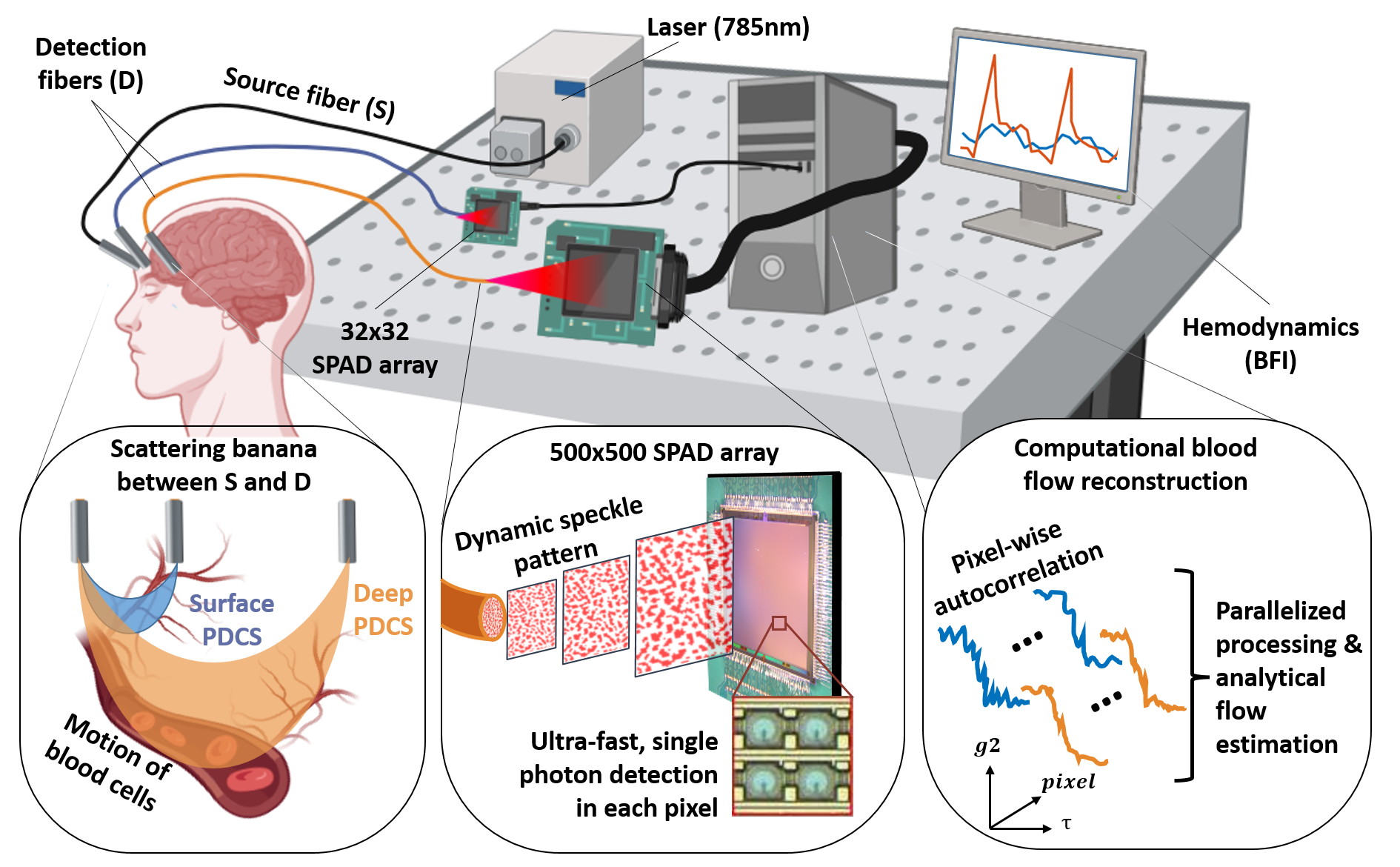
Figure 1: Basic principle and experimental setup of dual-detection pDCS. A coherent laser source is connected to an optical fiber which delivers light to the measurement location (e.g., the forehead for measurement of the cerebral blood flow). Photons are scattered from moving blood cells and travel along the ’banana-shaped’ path between source (S) and detection (D) fiber. Collected photons are transmitted an array of single-photon avalanche diodes (SPAD). One setup (blue fiber) is used at a short distance between S and D to measure superficial flow, while the second setup (orange fiber) collects light at a larger distance for deep flow measurement. Each pixel in the arrays measures a dynamic speckle pattern and time traces of these photon detection events are then used to compute autocorrelation curves. All parallelized DCS measurements are averaged to boost the signal-to-noise ratio in these autocorrelation curves before the blood flow index (BFI) and other hemodynamic metrics are deduced.

1 Introduction

Diffuse correlation spectroscopy (DCS) is a valuable, all-optical tool for quantifying blood flow dynamics at great tissue depths (>1cm), in a noninvasive, label-free fashion. This ability makes DCS especially appealing for applications in the field of neuroscience, with the aim to measure cerebral blood flow (CBF) beneath the barrier of the scalp and skull.

DCS is based on the analysis of speckle patterns, which are sensitive to particle motion. In biological tissues, this motion primarily reflects the dynamics of red blood cells. In a typical DCS setup, coherent laser light illuminates the sample at a defined location, while an optical fiber is placed at a known distance to the illumination spot to collect back-scattered photons (see Fig. 1). Photons that travel between the source (S) and detector (D) follow a path within a ’banana-shaped’, stochastic scattering profile (see Fig. 1 and Fig.2 b & c), where the largest depth is approximately half of the source detector separation (SDS) [1]. Thus, larger SDS leads to greater measurement depth. Most commonly, DCS is used at $SDS=2-2.5cm$) [2, 3, 4, 5, 6], relating to a measurement depth of $\sim 1-1.5cm$. In conventional DCS, only a small number of $\sim 1-8$ single ultra-fast detectors are used to measure the temporal changes of single speckles and the temporal intensity autocorrelation is calculated. Based on that, a blood flow index (BFI, cm2/s) can be derived using analytical models. Compared to the similar functional near-infrared spectroscopy (fNIRS), which is based on absorption instead of scattering, DCS has been reported to be more sensitive to CBF, since it directly measures the motion of blood cells instead of changes in blood volume [7].

Traditional DCS systems already significantly contributed to understanding blood flow dynamics in various clinical contexts, including Subarachnoid hemorrhage (SAH) [8], sickle cell disease (SCD) [2, 9], and delayed cerebral ischemia (DCI) [8]. DCS showed significant differences in the BFI of patients that suffered strokes [10] or in brain areas associated with speech of people who stutter [11] to name a few recent examples from the ever growing body of research.

Despite these successful applications, conventional DCS systems with only one or a few detection channels, are inherently constrained to a certain measurement depth, since the number of detected photons decreases significantly at greater depths.

Many different strategies have been used to address this limitation and increase the sensitivity of DCS, and thus ultimately increase its measurement depth and/or sampling rate. Interferometric setups, for instance, are sensitive to faster speckle variations, which is generally advantageous for DCS [12, 13, 14, 15]. Interferometric DCS, or interferometric diffusing wave spectroscopy (fiDWS), has been reported with source-detector separations of up to 4-5cm SD separation, but a relatively low sampling rate of 0.1 - 0.5 Hz (2-10 s integration time) [14].

A rather straight-forward method to increase the signal-to-noise ratio (SNR) in DCS is the simultaneous measurement of multiple, independent speckles. This concept has already been used conventional DCS for multi-speckle DCS [16], as well as in interferometric setups for ’highly parallel, interferometric diffusing wave spectroscopy’ by measuring $\sim$ 20 speckles in parallel [15].

The use of entire arrays with many individual SPAD pixels is among the latest innovations of this concept. For instance, Johansson et al. used a 5x5 SPAD array for ’multiplexed DCS’ [17] and Liu et al. showed ’parallelized DCS (pDCS)’, by using a 32x32 SPAD array  [18]. By pixel-wise averaging all of these independent autocorrelation curves, pDCS can consequently boost the SNR by a factor of $\sqrt{N_{pixels}}$ (e.g., up to 32-fold increase by averaging all 1,024 pixels in a 32x32 array) [18]. A similar pDCS setup with a 32x32 SPAD array was then used to classify spatiotemporal-decorrelating patterns deep beneath turbid media [19] and even to exploit such patterns to reconstruct images of flow patterns [20]. However, it should be noted, that the effective SNR-gain in pDCS compared to conventional DCS systems is usually slightly below the theoretical factor of $\sqrt{N}$, since SPAD arrays often have a lower photon detection efficiency (PDE) [21]. Therefore, larger SPAD arrays are needed to design pDCS systems that actually show a substantial SNR boost the SNR over existing DCS devices.

At the same time, the technical development of SPAD array technology has improved significantly; recently, a large-format 500x500 SPAD camera has been demonstrated [22]. Compared to the 32x32 array of 1,024 pixels, that was used for previous pDCS systems [18, 20, 19], this new SPAD array has almost 250-times more individual pixels (250,000 pixels compared to 1,024) and therefore offers capabilities for even more parallelized measurements (see Fig. 1). pDCS experiments on optical phantoms already validated that this massively parallelized SPAD array follows the same $\sqrt{N}$ gain in SNR, boosting it by a factor of up to 500 compared to single-pixel DCS, or by a factor of approximately 15 compared to the previous 32x32 pDCS [23]. While the promise of pDCS is evident, pDCS has only been tested on artificial tissue phantoms [18, 24, 23] or in preliminary studies on only a handful of human subjects (i.e., n=6) and at limited measurement depth [18]. Despite the very promising technological advance of the new 500x500 SPAD array [22, 23], SPAD cameras of this massive size have not yet been utilized to study actual blood flow in human subjects.

In this publication, we demonstrate the first use of a large-scale 500x500 SPAD camera for massively parallelized DCS in a large cohort of human subjects and under conditions highly relevant to neuro-cognitive studies. We show that this new system offers the ability to optically measure fast blood flow dynamics at great depth of approximately 2cm (SDS = 4cm), which is well beyond the measurement depth of conventional DCS at 1-1.5cm ($SDS=2-2.5cm$) [2, 3, 4, 5, 6], while still enabling fast sampling of pulsatile blood flow at 8-10Hz. We carried out a systematic study with 24 human subjects, investigating suppression as well as activation of blood flow. A dual-detection system with two different pDCS systems - one at short SDS and one at large SDS - further allowed a direct, in-built reference between superficial and deep tissue layers. Our results demonstrate the use of the latest SPAD array technology for massively parallelized DCS in biomedical and neuro-cognitive studies in general.

2 Methods

2.1 Study design

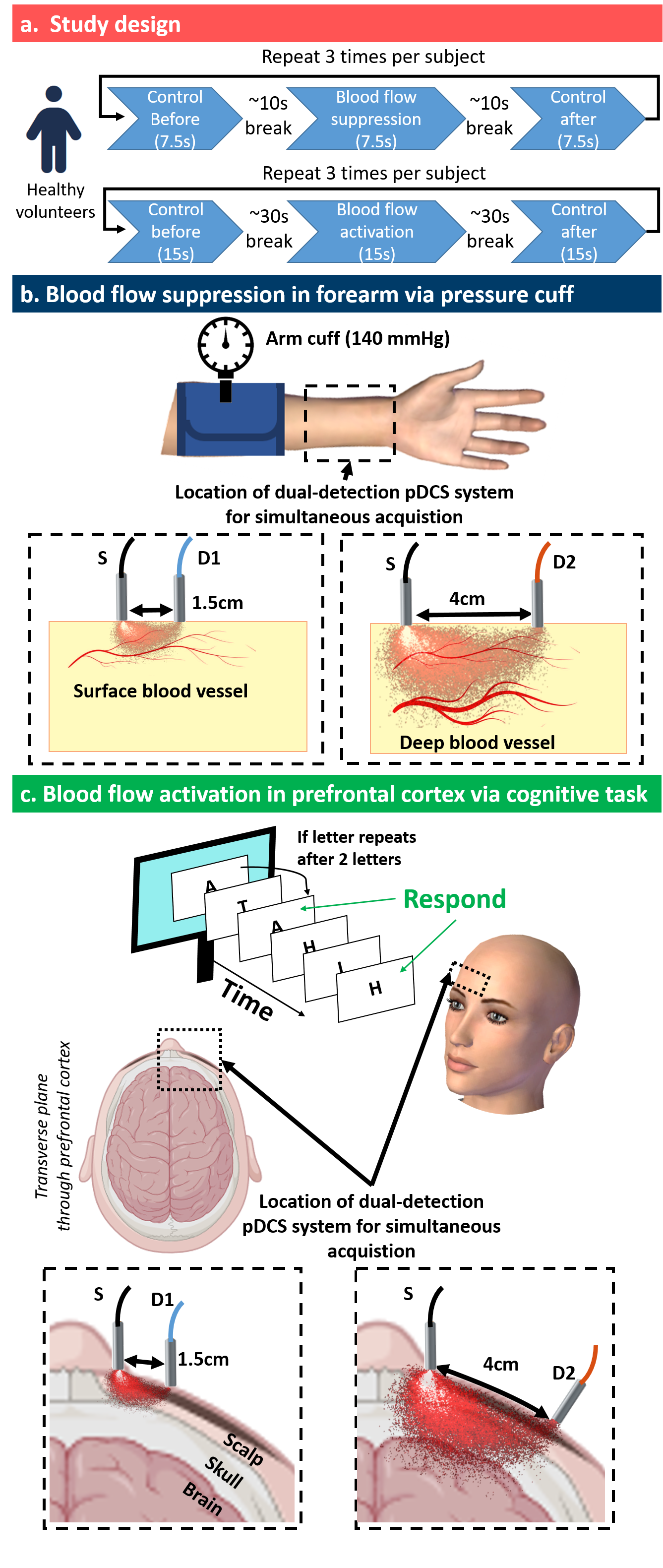
Figure 2: Study design and principle of dual-detection with pDCS at the forearm (b) and the forehead (c).

Healthy adult subjects (n = 24) were recruited for this study. To explore deep-tissue pDCS, data was collected from two different locations, under two different conditions: (i) general blood flow suppression in the entire forearm and (ii) localized activation of blood flow within brain tissue at the prefrontal cortex (PFC), behind the barrier of skin and skull tissue. At the forearm, pDCS data was collected before, during, and after blood flow suppression via a blood pressure cuff. At the PFC pDCS was recorded before, during, and after a cognitive activation task. The same procedure was repeated three times for three independent measurements per subject, as displayed in Fig. 2 a. We refer to these independent measurements as ’trials’. Participants were briefed about all details of the study, signed a consent form, and wore laser safety goggles throughout the entire experiment. The study protocol was approved by the Duke Campus Institutional Review Board (IRB) prior to the experiments (IRB Protocol Number 2022-0093).

pDCS measurement at the forearm during blood flow suppression

Subjects placed their right forearm on the table, and the optical setup consisting of three fibers was placed on the arm. A standard blood pressure cuff was placed on the upper arm of the subject. Three independent trials were recorded and each trial consisted of an initial control measurement without occlusion, one test measurement during occlusion, and a second control measurement seconds after the release of the pressure. Each measurement interval lasted 7.5s and there was a break of about 10s between two measurements (i.e., between control and occlusion measurement) to save the raw data to the drive. From the total number of 24 subjects, complete data from both detectors was available for 33 trials from 11 subjects. A pre-defined exclusion criterion for the residual of BFI estimation was applied to this data and resulted in the removal of nine trials, following the pre-registered analysis plan at https://doi.org/10.17605/OSF.IO/TJ2WV.

pDCS measurement at the prefrontal cortex during cognitive activation

For these measurements, subjects placed their head on a chin rest. Three optical fibers were positioned at the forehead, 1-2 cm above the right eyebrow to measure the blood flow in the underlying tissue. A small monitor was placed at about 20 cm distance at eye level of the subject and their hands were placed on a keyboard to control the required keys for the cognitive task. The n-back task (n = 2) was carried out on a web service provided by PsyToolkit’s experiment library at https://www.psytoolkit.org/experiment-library/nback2.html [25, 26]. This task activates brain areas for short-term memory and action planning, located in the PFC [27]. During this task, a series of 25 letters is shown to the participants, usually containing six instances, where the same letter is repeated after two letters (see Figure 2 c). Prior to the actual experiment, each subject was instructed in the procedure and the rules of this n-back test. Each subject carried out one practice test, without data acquisition to familiarize themselves with the test. If subjects correctly indicated this instance, it was counted as a correct match. Missed instances and false alarms were also counted. The percentage of correct matches, the percentage of missed matches, and the percentage of false alarms were documented for each trial. Each trial consisted of an initial control measurement, followed by a measurement during the task and, finally, another control measurement (see Fig. 2 a). The entire test lasted about 40-50s and the pDCS measurement was started about 15-20s after the start of the test. Each pDCS measurement lasted 15s. After the task was completed, subjects were again asked to close their eyes and a second control measurement was recorded. There was a break of about 20-30s between two measurements in the same trial (i.e., between control measurement and task measurement). The same procedure was repeated three times, to obtain three independent trials for each subject. From the total number of 24 subjects, complete data from both detectors was available from 48 trials. Nine trials of the cognitive task were excluded based on the pre-defined exclusion criterion for the residual of the BFI reconstruction for a total of 39 trials from 15 subjects.

2.2 Optical setup

As displayed in Fig. 1 and in Fig. 2 b & c, we used a dual pDCS system, with one laser source ($\lambda=785nm$) and two individual detection setups. The laser was operated at 100mW and connected to a large fiber patch cable (Thorlabs M107L, $1500\mu m,NA=0.50$). An empty lens tube with a length of 16mm was mounted to the laser fiber to act as a spacer between the fiber tip and the subject’s skin. This ensured a sufficiently large beam diameter at the skin and an intensity well below the maximal permissible exposure (MPE) limit of 300 mW/cm².

The first detection setups consisted of the commercially available 32x32 SPAD camera (PF32, PhotonForce Ltd., Scotland, UK) that was connected to a 200 µm fiber (Thorlabs M44L, $200\mu m,NA=0.50$), at 1.5 cm distance to the laser fiber (SDS = 1.5 cm). The second setup was based on the novel 500x500 SwissSPAD3 array [22], connected to a 1500 µm fiber (Thorlabs M107L, $1500\mu m,NA=0.50$), at a distance of 4cm to the laser fiber (SDS = 4 cm). In both cases, the distance between the fiber end and the sensor (z) was adjusted to match the speckle diameter (d) to the active area of the detector, according to [28]:

$$d=\frac{\lambda z}{D}$$ (1)

where $\lambda$ is the wavelength (785 nm) and D is the fiber diameter. In the case of the setup with the short source-detector separation (SDS = 1.5cm), the diameter of the active area of each pixel in the PF-32 array is 6.9 $\mu m$, resulting in a distance of z = 1.76 mm between fiber and detector. In the case of the long source-detector separation (SDS = 4 cm), the setup followed the procedure described by Wayne et al. [23], with a distance of z = 11.5 mm between fiber and detector, since the diameter of the active area of each pixel in the SwissSPAD3 array is 6 $\mu m$. To ensure a correct setup, the speckle patterns at these distances were measured by a camera with $1.85\mu m$ pixel size (acA4024-29um, Basler AG, Ahrensburg, Germany).

2.3 Data processing

DCS measurements are based on the temporal autocorrelation curve, given by:

$$g_{2}(\tau)=\frac{\langle I(t)*I(t+\tau)\rangle}{\langle I(t)\rangle^{2}}$$ (2)

where the brackets $\langle\rangle$ denote time averages, $\tau$ denotes the time delay variable of the temporal autocorrelation and I(t) is the measured number of binary photon detection events. In each case, this $g_{2}$ was calculated based on Equ. 2 individually per pixel of the sensor. The system offered two different modes of operation to obtain the $g_{2}$ data: (1) streaming of full raw frame data. This data was transferred via an iPASS cable (IPASS PCIE CABLE ASSY 68P 3M, 0745460801, Molex, Wellington, USA) that was connected to a PCIE cable assembly expansion board (AVT-ONIX-PCIE-IPASS-8X-G board, Onix systems, Israel), saving full frame data to a SSD hard drive or (2) automated, real-time, on-board calculation of the $g_{2}$ curves on the respective FPGA unit. The FPGA firmware was developed by Wayne et al. [23] and outputs $g_{2}(\tau)$ values over a USB3.0 connection at 16 delay times, between $\tau_{0}=0$ (no delay) and $\tau_{max}$ at 15 times the exposure time.

The temporal resolution $\Delta\tau$ of these $g_{2}$ curves is defined by the total exposure time of each sensor. The 32x32 PF-32 detector has a global shutter and the exposure time was held constant at 3 $\mu s$ in all experiments. The larger 500x500 swissSPAD3 detector has a rolling shutter and the number of readout rows can be adjusted. Thus, its full-frame exposure time is defined by the number of rows that is read, multiplied by the readout time for each row of 40ns [22, 23]. In the full raw data streaming mode, the number of rows could be adjusted freely between 1 and 250, for a full-frame exposure time of $t_{exposure}=n_{rows}\times 40ns$. The on-board autocorrelation mode only allowed measurements of either 250 rows from one sensor half at $10.81\mu s$ exposure ($250\times 40ns=10\mu s$, plus additional wait time for wait states and clock cycle) or 64 rows from two sensor halves (128 rows in total) at $3.37\mu s$ exposure ($64\times 40ns=2.56\mu s$, plus additional wait time). For the experiments described in this work, two different settings were used, tailored to the specifications of the experiment. In each case, $g_{2}$ was calculated for each individual SPAD pixel and then all curves were averaged across all pixels to boost the SNR as described previously [18, 23]. Furthermore, $g_{2}$ curves were averaged within a certain time window, which defined the temporal sampling of the blood flow metrics, as specified below.

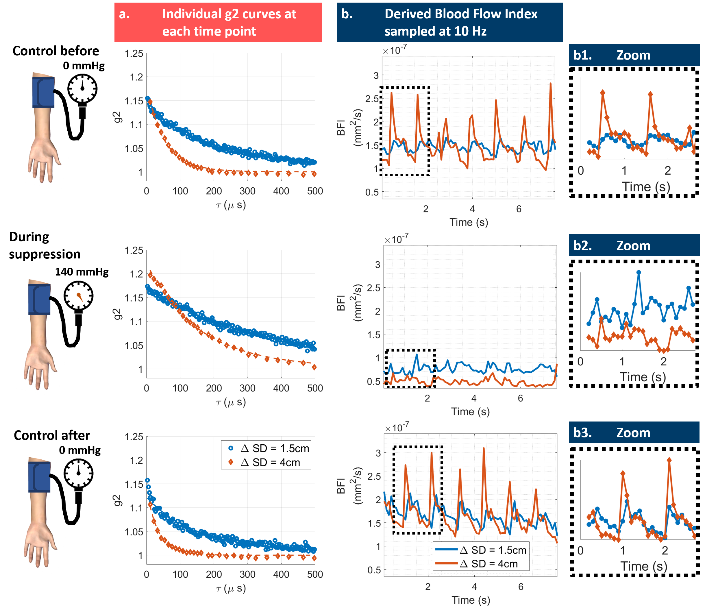
Figure 3: PDCS measurement at the arm of an exemplary subject before, during, and after blood flow suppression via occlusion. (a) Points represent individual $g_{2}$ values, the fit by the analytical diffusion model is shown as a dotted line. (b) The derived BFI trace over time, sampled at 10 Hz. (b1) A zoomed inlet shows each BFI value as a point. The arrow marks the value that was derived by the $g_{2}$ curve shown as ’Control 1’ in (a).

BFI estimation by correlation diffusion model

All calculated $g_{2}$ curves were used to estimate the blood flow index (BFI), according to the semi-infinite solution to the correlation diffusion equation, which has been described extensively in literature [29, 30, 31, 32, 33, 34]. We used publicly available code for this model from Wu. et al. [35].

In brief, $g_{1}$ was calculated analytically as a function of BFI and $\beta$, as well as based on a few basic assumptions of optical properties. Then $g_{1}$ is then inserted into the Siegert relation [36]:

$$g_{2}=1+\beta*|g_{1}|^{2}$$ (3)

This analytical $g_{2}$ model is fitted to the measured $g_{2}$ data obtained at each time point, by optimizing for BFI and $\beta$. Finally, the goodness of the fitted semi-infinite diffusion correlation model was analyzed by considering its residuals. The mean residual per trial was analyzed and a threshold for the median residual of 0.03 was used to exclude outliers from further statistical analysis described below.

Additional blood flow metrics

Besides the rigorous and established BFI, the initial $g_{2}$ difference was tested for blood flow sensitivity. The rationale for this metric is that it carries information on changes in speckle contrast, similar to rBFI, but only considering the two earliest delay values at highest blood flow sensitivity. Since the $g_{2}$ curve decayed relatively fast at this large SDS (see Fig. 3 and 4), the initial difference between the first two decay values was tested as an additional metric of potential blood flow sensitivity:

$$\Delta g_{2,init}=g_{2}(\tau_{1})-g_{2}(\tau_{2})$$ (4)

This initial $g_{2}$ difference was sampled at the same rate as the BFI (8 Hz for the cognitive activation experiment and 10 Hz for the suppression experiment).

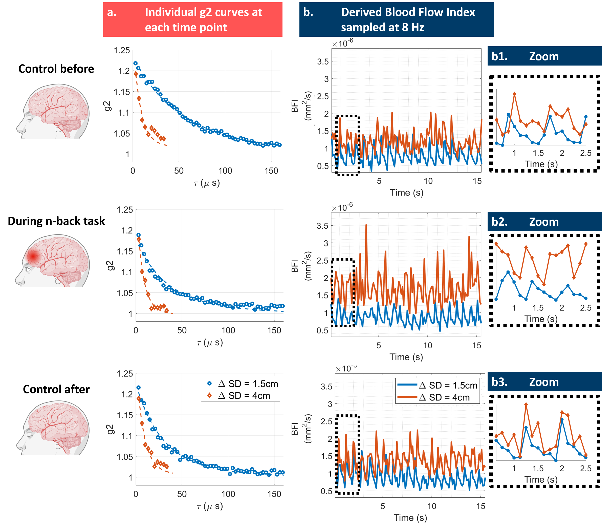
Figure 4: PDCS measurement at the prefrontal cortex of an exemplary subject before, during, and after a cognitive task. (a) Points represent individual $g_{2}$ values, the fit by the analytical diffusion model is shown as dotted line. (b) The derived BFI trace over time, sampled at 8 Hz. (b1) A zoomed inlet shows each BFI value as point. The arrow marks the value that was derived by the $g_{2}$ curve shown as ’Control 1’ in (a).

2.4 Statistical analysis

For each trial, the data was normalized to 100% of the median of the first control measurement. The data from each of the two detectors was analyzed separately so that the short source-detector separation (SDS = 4cm) could serve as an in-built control measurement for the deep pDCS configuration (SDS = 4cm).

For each individual trial, the median of the time course (e.g., rBFI(t)) was calculated for the first control, the test condition (suppression by cuff or activation by cognitive task), and for the second control. The group distribution of these median values in all trials was plotted and analyzed by a linear mixed effects (LME) model to derive p and t values. The LME used the normalized, averaged blood flow metric as the outcome variable while using the trial and the condition (control or experimental) as predictor variables with a random intercept and slope for each trial:

$$rBFI\sim Trial+Condition+(Condition|Subject)$$ (5)

We ran the same analysis for both sensors to compare blood flow changes that were recorded simultaneously from superficial and deeper tissue layers. Furthermore, the average difference and Cohen’s difference [37] of the distribution were calculated. The same procedure was also applied to the other two metrics (Intensity and initial $g_{2}$ difference, see sub-chapter 2.3 above for more details on those metrics). This analysis procedure follows the pre-registered study design at https://doi.org/10.17605/OSF.IO/TJ2WV.

3 Results

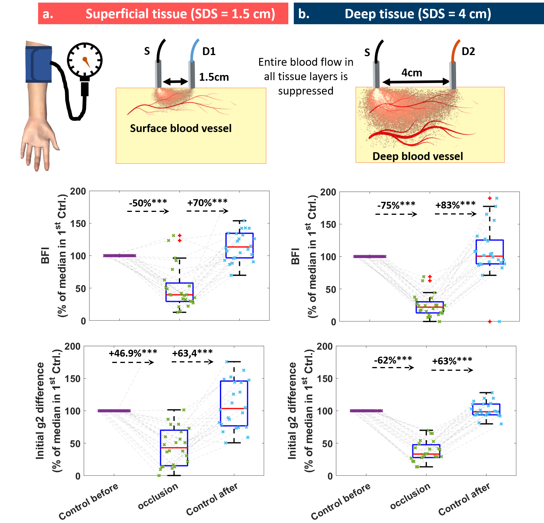
Figure 5: Group PDCS data from blood flow suppression via occlusion. (a) Superficial signal at 1.5cm source-detector separation. (b) Deep signal at 4cm source-detector separation. Both metrics (BFI and initial $g_{2}$ slope) show a statistically significant decrease during blood flow suppression via occlusion (*p<0.05 for all cases). All boxplots show the 25th and 75th percentile as blue boxes. Values denote the average group difference. Significance levels are indicated as *p<0.05, **p<0.01, ***p<0.001.

3.1 pDCS measurements during blood flow suppression in soft tissue

As expected, the $g_{2}$ curves decay much faster in the pDCS measurements at larger source-detector separation compared to shorter source-detector separation under the same conditions (see Fig. 3 a). For both pDCS configurations (SDS = 1.5cm and SDS = 4cm), the derived BFI values (Fig. 3 b) clearly show the characteristic diastolic and systolic peaks that are typically present in arteries [38], which confirms blood flow sensitivity for superficial and deep tissue measurements. The pulses in both measurements indicate a fairly similar pulse frequency of about 1-1.3Hz (60-80bpm), which is within the expected physiological range for healthy adults [38]. The superficial pDCS measurement shows lower pulse BFI peak values than the deep pDCS measurement, which is expected since the BFI is related to the blood velocity, which is high in the larger arteries but drops in the smaller capillaries [38], that are closer to the surface of the skin. The superficial pDCS recordings at about 0.5-0.75cm measurement depth target a relatively larger number of capillaries and fewer larger arteries compared to the deep pDCS configuration at 2cm depth. Upon suppression of blood flow via a pressurized arm cuff (center column in Fig. 3 a-c), the $g_{2}$ curves show a later decay and the derived BFI time traces show a significantly decreased BFI value overall and no pulsatile behavior, indicating the lack of moving blood cells.

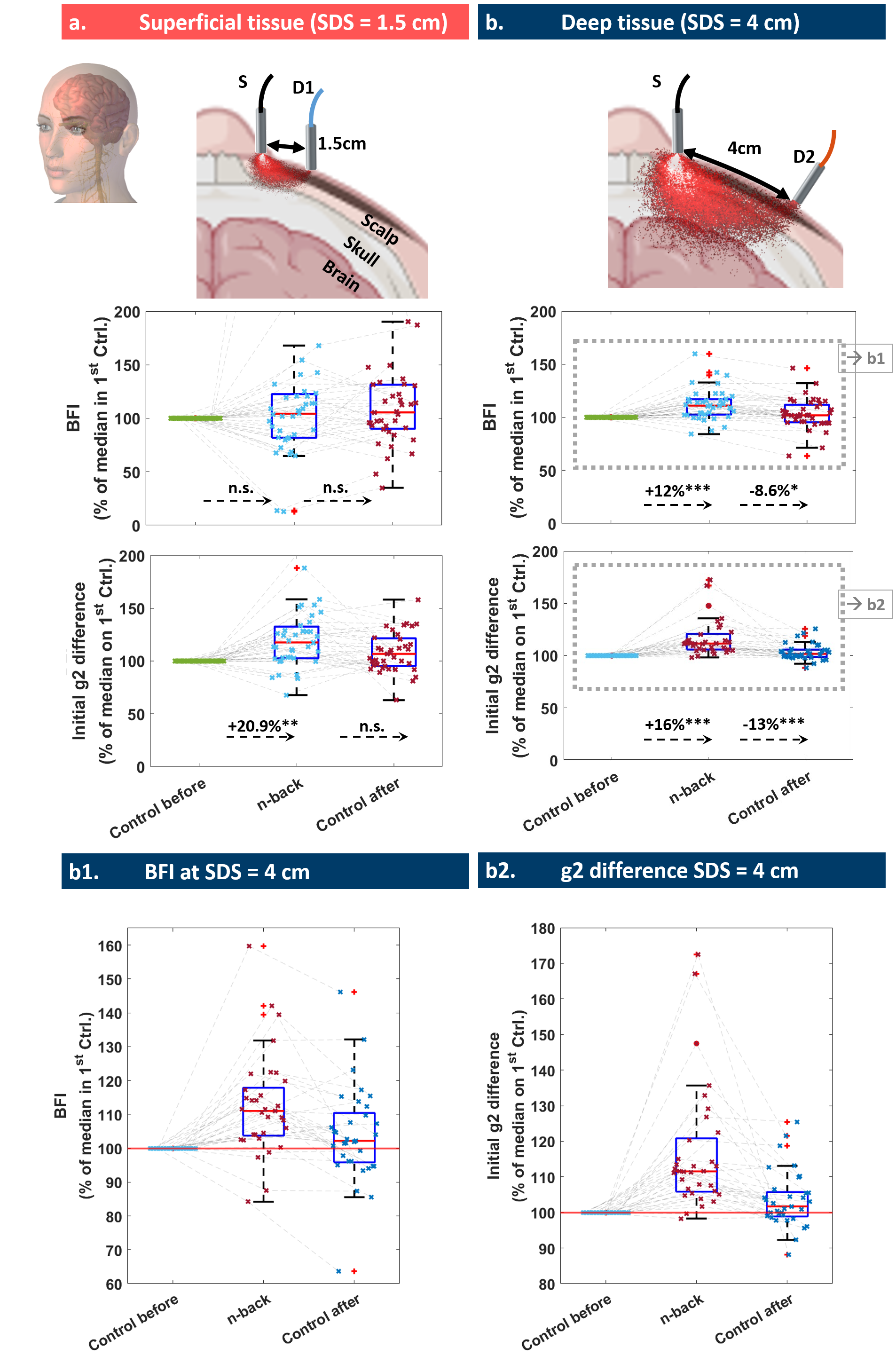
Figure 6: Group PDCS data from cognitive activation task. (a) Signals at SDS=1.5cm shows no statistically significant change (except for initial slope metric compared to first control), since the most scattered photons at this configuration ado not reach brain tissue. (b) Deep signal at SDS=4cm: all metrics show a statistically significant increase during activation via a cognitive task. (b1 & b2) show re-scaled versions of the group differences from the deep tissue layer (at SDS=4cm). All boxplots show the 25th and 75th percentile as blue boxes. Values denote the average group difference. Significance levels are indicated as *p<0.05, **p<0.01, ***p<0.001.

3.2 pDCS measurements during blood flow activation in the brain

Similar to the previously reported results from the forearm, the $g_{2}$ curves from the forehead generally decay much faster at larger SDS (see Fig. 4 a), the derived BFI values (Fig. 4 b) show pulsatile blood flow at both configurations (SDS = 1.5cm and SDS = 4cm) and the peak pulse BFI is higher for the deep pDCS measurement compared to the BFI at superficial pDCS recordings. Again, the pulse frequency is similar for both measurements at about 1 - 1.5Hz (60-90bpm) and within the expected physiological range. In contrast to the results from the previous suppression experiment, the $g_{2}$ curves at larger SDS experience more noise, especially towards longer delay values, as seen in Fig. 4 a. This justifies the choice to only use the initial 12 delay values ($\tau=3.3-40.4\mu s$) for the diffusion model to derive BFI, as explained above in paragraph 2.3. In contrast to the results in the previous experiment, the derived BFI values (Fig. 4 b) are generally higher for longer source-detector separation, which might indicate cerebral sensitivity, since it has been reported that BFI can be up to 6 to 10 times higher in the brain as in the surrounding tissue [7]. During the active cognitive task (center column in Fig. 4 a-c) the BFI at large source-detector separation (SDS = 4cm) clearly shows an overall increase compared to the control measurement, while the BFI at SDS = 4cm shows little to no effect under the same condition. As shown in Fig. 2 c, this trend is expected if brain sensitivity was reached, as the scattering banana at SDS = 4cm only allows a tiny fraction of photons to penetrate scalp and skull, while a substantially larger number of photons reach the brain at the larger SDS.

3.3 Statistical analysis of group results

Fig. 5 shows the grouped pDCS results from all trials in the blood flow suppression experiment at superficial tissue layers (subpanel a) and at deep tissue layers (subpanel b). The results in these group statistics follow the general trend as described above for the BFI time trace in an individual trial in Fig. 3. For the superficial pDCS measurement, the suppression of blood flow in the forearm via a pressurized cuff resulted in a highly significant decrease of an average of 50 % in normalized BFI, when compared to the first control. Upon release of the pressure (’Control after’), the normalized BFI reached an average of around 120 %, indicating that the normalized BFI exceeded the initial level during reactive hyperemia (i.e., when the blood rushed back). For the deep tissue pDCS measurement, this change is also highly significant but stronger in magnitude, reaching an average decrease of 75 % during suppression when compared to the control before or an average difference of 83 % when compared to the control after.

In a similar fashion, Fig. 6 shows the respective pDCS results in the cognitive activation experiment. Again, the results in these group statistics follow the general trend as described above for the BFI time trace in an individual trial in Fig. 4. For the superficial pDCS measurement, the change in normalized BFI is slightly positive but did not reach statistical significance. Only in the deep tissue pDCS configuration, which actually enables cerebral sensitivity, does this increase in normalized BFI reach clear statistical significance with an average increase of 12 % and 8 %, when compared to the control before or after the cognitive task, respectively.

3.4 Test of an additional potential flow parameter

As presented in section 2.3, we further tested the initial $g_{2}$ difference in addition to the more rigorous and well-established BFI. As shown in Fig. 6, this metric follows the same general trend in the group statistics as the rBFI described above - albeit at a different magnitudes. For the superficial tissue measurement in the forearm, this metric shows a highly significant decrease of 46 % and 63 % when compared to the control before or after, respectively. For the deep tissue pDCS measurement in the same experiment, the average decrease of this metric is 62 % and 63 %. In the cognitive experiment, this metric of initial $g_{2}$ difference in the deep pDCS configuration shows a statistically significant, average increase of 15 % and 12 %, when compared to the control before or after, respectively. For the superficial pDCS configuration, the metric even reaches statistical significance, when comparing the control before with the test condition at an average increase of 20 %, but no significant change when compared to the control after. Although this trend is apparent and statistically significant, this large difference in average value of >60% for the arm or >15% in the PFC should not be mistaken for a equivalently large difference in measured flow. The magnitude of this change is not linearly proportional to actual blood flow changes, since it might be affected by several other parameters, like changes in absorption (e.g., due to increased hemoglobin volume), natural fluctuations $\beta$ and others.

4 Discussion and Conclusion

This study leveraged parallelized Diffuse Correlation Spectroscopy (pDCS) with the cutting-edge 500x500 SwissSPAD3 camera, demonstrating cerebral blood flow sensitivity. To the best of our knowledge, this accomplishment marks the first in vivo application of 500x500 SPAD array technology for pDCS in human subjects. The study showcases the success of massively parallelized DCS at a large SDS of 4 cm and fast sampling rates of 8-10Hz. Our results showed the expected increase in blood flow dynamics during cognitive activation only in the deeper regions of the PFC, while the reference measurement at shorter SDS confirmed no significant change. Contrarily, our system accurately showed the global decrease in blood flow in superficial and deep tissue layers of the forearm upon suppression by a pressurized cuff. All results showed adequate statistical significance in a large group of healthy human volunteers.

Trade-off between SNR, temporal resolution, and photon detection

The fidelity of massively parallelized DCS is governed by the trade-off between temporal resolution, signal-to-noise ratio (SNR), and photon detection. The term ’temporal resolution’ relates to two rather different concepts in (p)DCS: the exposure time of each SPAD pixel, defining the temporal resolution of the $g_{2}$ curves ($\Delta\tau$), and the temporal resolution of the BFI time trace defined by the averaging window. The resolution of the $g_{2}$ curve, $\Delta\tau$, is essential for measurements several centimeters deep within tissue, as the average number of scattering events increases towards many thousands, which causes the temporal speckle fluctuations to increase to the MHz regime. The temporal averaging window, on the other hand, defines the rate at which blood flow changes can be sampled at a given SNR. The rolling shutter of the SwissSPAD3 array defines the total exposure time by the number of rows that are read out. More rows allow more parallelized measurements and thus higher SNR, but result in longer exposure times, which reduces the $g_{2}$ resolution (increased $\Delta\tau$) and inhibits flow sensitivity. Our results from the arm experiment, comparing the massively parallelized SPAD array (250x500) with the conventional PF-32 array, demonstrated a 122-fold increase in available pixels and thus an estimated 11-fold increase in SNR, when assuming similar PDE for both arrays (diameter of the active sensor area is similar for both arrays with $6.9\mu m$ for PF-32 and $6\mu m$ for swissSPAD3). However, this came at the cost of reduced temporal resolution of the $g_{2}$ curves for the larger array of $10\mu s$ compared to the $3\mu s$ of the smaller PF-32. Nevertheless, both detectors still adequately captured the autocorrelation decay in the forearm. This situation is rather different in the deep pDCS measurement from the prefrontal cortex (PFC), where the flow is faster and thus the autocorrelations decay earlier. Therefore, only 128 SPAD rows for a total of 64,000 SPAD pixels from the swissSPAD3 array were read out to increase the temporal resolution (decrease $\Delta\tau$) of the $g_{2}$ curves. Additionally, the calculation of autocorrelation was performed onboard, at a fixed amount of 15 decay values. This approach resulted in a shorter range of delay values and a lower number of consecutive frames for each $g_{2}$ curve. Therefore, the averaging window of 0.128s resulted in a much higher number of averaged $g_{2}$ curves as compared to the PF-32 measurement in the same experiment, while still maintaining similar exposure times, and therefore a similar $\Delta\tau$, for both arrays ($3.37\mu s$-vs.- $3\mu s$).

Dual detection in pDCS: "A bunch of bananas"

The utilization of two different detectors at distinct SDS facilitated the comparison of superficial flow changes with flow changes in deeper tissue. Thereby, the second detector at short SDS served as an in-build reference measurement under the exact same conditions. Generally, the deep pDCS configuration is sensitive to blood flow within the volume of the entire scattering banana, including superficial as well as deeper layers (e.g., extracerebral tissue of scalp and skull as well as cerebral tissue in the brain). In contrast to that, the pDCS signal at short SDS is dominated by contributions from the superficial tissue layers (e.g., extracerebral). Thereby, our dual detection scheme allowed to rule out other potential causes for increased blood flow, not assigned to cerebral activity, such as eye motion or motion artifacts. While similar approaches of using multiple detection systems for different measurement depths have been used in conventional DCS [3, 2, 39], its application in pDCS with entire arrays of SPADs is new. Due to this dual-detection scheme, we were able to show that the cognitive task only induced a significant increase of blood flow metrics from the deep tissue pDCS measurement that actually reached brain tissue, while yielding no significant changes at superficial layers of skin and skull. In contrast to that, the global blockage of blood flow in the forearm via a pressure cuff showed a significant decrease in blood flow metrics in both tissue layers.

In the future, more sophisticated data processing techniques might even be able to leverage such dual-detection pDCS data to correct the deep measurement by the extracerebral background and obtain an informed estimation of the signal that arises purely from the cerebral tissue at greater depth. Attempts to minimize the extracerebral contributions on deep measurements (i.e., from scalp and skull) are commonly used for fNIRS and some attempts have already been made to translate this approach to DCS [39, 34]. Thereby, general linear models (GLM) are used to regress out the relative changes in BFI at short SDS (i.e., scalp hemodynamics) from the relative changes in BFI at long SDS (i.e., hemodynamics in scalp and brain). Alternatively, more complex multi-layer diffusion correlation models have been explored for DCS [39]. Although these methods are valid for fNIRS, which essentially measures changes in blood volume, they faces unique challenges for DCS, which measures blood flow velocity. While the volume flow of blood remains relatively constant across different types of vessels, the flow velocity changes substantially between arteries, arterioles, capillaries, and veins, due to the differences in vessel diameter, wall thickness, and overall flow resistance [38]. Indeed, our experimental results from the forearm found a reduced BFI peak pulse at the superficial pDCS measurements, indicating a higher ratio of smaller capillaries (slower flow velocity) within the scattering banana at SDS = 1.5cm and a more pronounced pulsating behavior at the deep pDCS measurements (SDS = 4cm), indicating that the measurement reached more of the larger arteries in deeper tissue layers. To understand how exactly DCS signals from different tissue layers are mixed, and thereby establish better mixture models, like GLMs, additional information about the vasculature at the respective tissue depth, as well as mathematical models on how this vasculature shapes the flow dynamics, are required. Therefore, it has been reported that such multi-layer models "should be taken with caution" and that the homogeneous model performs better under general assumptions [40].In future studies, complementary imaging techniques, like Doppler ultrasound or magnetic resonance imaging (MRI) could provide information the vascular morphology in each layer, while fluid dynamic simulations might inform how that morphology shapes the blood flow velocity. In the future, we expect that such a multi-modal approach would be able to fully leverage data from our dual-detection pDCS setup and lift its potential for a more informed estimation of isolated deep flow, corrected by the contribution from superficial tissue layers.

Limitations and challenges

The study acknowledges potential limitations and challenges in terms of the underlying biology, the technical setup, and the data processing. For instance, there is a natural, biological variance in scalp and skull thickness between different subjects (average thickness of scalp and skull is approx. $1.48\pm 0.28cm$ [41]), while the depths of the scattering banana at SDS = 4cm is roughly 1.3-2cm. Under these considerations, the number of photons that reach brain tissue would vary significantly between different subjects of different scalp and skull thickness and thus, our described methodology might yield varying cerebral sensitivity for each individual subject. With respect to the technical setup, we recognize the exposure time of $3\mu s$ as a limitation in sampling the very fast correlation decay in brain tissue. Although our results indicate blood flow sensitivity in cerebral tissue, a higher frame rate (lower exposure time) of SPAD arrays would be desirable to capture earlier delay values and to obtain a better temporal resolution of the autocorrelation function, which would probably enhance blood flow sensitivity. Finally, the use of the same optical parameters for all subjects in the modeling of $g_{2}$ curves to derive BFI values is a limitation related to the data processing pipeline. Since optical properties were not measured during this study, we relied on reasonable estimations commonly used in literature. However, the absorption parameter $\mu_{a}$, in particular, has been described to vary largely between different skin color types (i.e., a 5-fold difference in melanin concentration) [42] and should be taken into account for each subject specifically in the future.

Outlook

Already in 2020, a one Mpixel SPAD camera was reported, albeit at a relatively low frame rate of 24 kfps [43]. This study used a SPAD camera with 0.25 Mpixel at 100-300kfps [22]. It is very likely that the ongoing development of SPAD camera technology will result in larger and faster detectors in the future, which would allow to sample the $g_{2}$ curves at higher temporal resolution (smaller $\Delta\tau$) for higher blood flow sensitivity, while also allowing even more parallelized DCS measurements to increase the SNR even further. These advances would allow higher sampling rates (smaller averaging windows) of the blood flow metrics, higher temporal resolution of blood flow dynamics and ultimately allow even deeper DCS measurements. In addition to that, new data processing techniques, tailored for the sparse signal of binary photon detection events in SPAD detectors are an anticipated refinement for the future. This study provides experimental evidence in using massively parallelized SPAD cameras to measure cerebral blood flow in vivo and therefore lays the groundwork towards advancing physiological research and clinical diagnostics in the future.

5 Backmatter

Funding R.H. acknowledges support from a Hartwell Foundation Individual Biomedical Researcher Award. This material is based upon work supported by the Air Force Office of Scientific Research under award number FA9550-21-1-0401. Mi.Wa. acknowledges partial support by the Swiss National Science Foundation (grant 20QT21-187716 Qu3D “Quantum 3D Imaging at high speed and high resolution”) and by Meta Platforms Inc.

Acknowledgments We thank Nir Beckermus and his team at Beckermus Technologies ltd for their support during this project. Furthermore, we are grateful to Dr.-Ing. Paul Ritter and Dr. Kyle Cowdrick for the valuable discussions on blood flow dynamics.

Disclosures M.W., R.H. and L.K. have submitted a patent application related to this work, assigned to Duke University. Edoardo Charbon holds the position of Chief Scientific Officer of Fastree3D, a company making LiDARs for the automotive market, and Claudio Bruschini and Edoardo Charbon are co-founders of Pi Imaging Technology. Neither company has been involved with the work or paper. The authors declare no other competing financial interests. All other authors declare no conflicts of interest.

Data Availability Statement The code for the diffusion model was based on the scatterBrains project from Wu. et al. [35] that is publicly available at https://github.com/wumelissa/scatterBrains.

6 References

References

References

- [1] T. Durduran, R. Choe, W. B. Baker, and A. G. Yodh, “Diffuse optics for tissue monitoring and tomography,” \JournalTitleReports on progress in physics 73, 076701 (2010).
- [2] S. Y. Lee, K. R. Cowdrick, B. Sanders, et al., “Noninvasive optical assessment of resting-state cerebral blood flow in children with sickle cell disease,” \JournalTitleNeurophotonics 6, 035006–035006 (2019).
- [3] L. N. Shoemaker, D. Milej, J. Mistry, and K. St. Lawrence, “Using depth-enhanced diffuse correlation spectroscopy and near-infrared spectroscopy to isolate cerebral hemodynamics during transient hypotension,” \JournalTitleNeurophotonics 10, 025013–025013 (2023).
- [4] W. Lin, D. R. Busch, C. C. Goh, et al., “Diffuse correlation spectroscopy analysis implemented on a field programmable gate array,” \JournalTitleIEEE Access 7, 122503–122512 (2019).
- [5] W. B. Baker, A. B. Parthasarathy, K. P. Gannon, et al., “Noninvasive optical monitoring of critical closing pressure and arteriole compliance in human subjects,” \JournalTitleJournal of Cerebral Blood Flow & Metabolism 37, 2691–2705 (2017).
- [6] R. Choe, M. E. Putt, P. M. Carlile, et al., “Optically measured microvascular blood flow contrast of malignant breast tumors,” \JournalTitlePloS one 9, e99683 (2014).
- [7] J. Selb, D. A. Boas, S.-T. Chan, et al., “Sensitivity of near-infrared spectroscopy and diffuse correlation spectroscopy to brain hemodynamics: simulations and experimental findings during hypercapnia,” \JournalTitleNeurophotonics 1, 015005–015005 (2014).
- [8] E. Sathialingam, K. R. Cowdrick, A. Y. Liew, et al., “Microvascular cerebral blood flow response to intrathecal nicardipine is associated with delayed cerebral ischemia,” \JournalTitleFrontiers in Neurology 14, 1052232 (2023).
- [9] K. Cowdrick, M. Akbar, T. Boodooram, et al., “Impaired cerebrovascular reactivity in pediatric sickle cell disease using diffuse correlation spectroscopy,” \JournalTitleBiomedical Optics Express (2023).
- [10] R. C. Mesquita, T. Durduran, G. Yu, et al., “Direct measurement of tissue blood flow and metabolism with diffuse optics,” \JournalTitlePhilosophical Transactions of the Royal Society A: Mathematical, Physical and Engineering Sciences 369, 4390–4406 (2011).
- [11] G. M. Tellis, R. C. Mesquita, and A. Yodh, “Use of diffuse correlation spectroscopy to measure brain blood flow differences during speaking and nonspeaking tasks for fluent speakers and persons who stutter,” \JournalTitlePerspectives on Fluency and Fluency Disorders 21, 96–106 (2011).
- [12] J. Xu, A. K. Jahromi, J. Brake, et al., “Interferometric speckle visibility spectroscopy (isvs) for human cerebral blood flow monitoring,” \JournalTitleAPL Photonics 5, 126102 (2020).
- [13] M. Zhao, W. Zhou, S. Aparanji, et al., “Interferometric diffusing wave spectroscopy imaging with an electronically variable time-of-flight filter,” \JournalTitleOptica 10, 42–52 (2023).
- [14] W. Zhou, O. Kholiqov, J. Zhu, et al., “Functional interferometric diffusing wave spectroscopy of the human brain,” \JournalTitleScience advances 7, eabe0150 (2021).
- [15] W. Zhou, O. Kholiqov, S. P. Chong, and V. J. Srinivasan, “Highly parallel, interferometric diffusing wave spectroscopy for monitoring cerebral blood flow dynamics,” \JournalTitleOptica 5, 518–527 (2018).
- [16] K. Murali and H. M. Varma, “Multi-speckle diffuse correlation spectroscopy to measure cerebral blood flow,” \JournalTitleBiomedical Optics Express 11, 6699–6709 (2020).
- [17] J. D. Johansson, D. Portaluppi, M. Buttafava, and F. Villa, “A multipixel diffuse correlation spectroscopy system based on a single photon avalanche diode array,” \JournalTitleJournal of biophotonics 12, e201900091 (2019).
- [18] W. Liu, R. Qian, S. Xu, et al., “Fast and sensitive diffuse correlation spectroscopy with highly parallelized single photon detection,” \JournalTitleAPL Photonics 6, 026106 (2021).
- [19] S. Xu, W. Liu, X. Yang, et al., “Transient motion classification through turbid volumes via parallelized single-photon detection and deep contrastive embedding,” \JournalTitleFrontiers in neuroscience 16 (2022).
- [20] S. Xu, X. Yang, W. Liu, et al., “Imaging dynamics beneath turbid media via parallelized single-photon detection,” \JournalTitleAdvanced Science 9, 2201885 (2022).
- [21] E. James and P. R. Munro, “Diffuse correlation spectroscopy: A review of recent advances in parallelisation and depth discrimination techniques,” \JournalTitleSensors 23, 9338 (2023).
- [22] M. Wayne, A. Ulku, A. Ardelean, et al., “A 500 500 dual-gate spad imager with 100% temporal aperture and 1 ns minimum gate length for flim and phasor imaging applications,” \JournalTitleIEEE Transactions on Electron Devices 69, 2865–2872 (2022).
- [23] M. A. Wayne, E. J. Sie, A. C. Ulku, et al., “Massively parallel, real-time multispeckle diffuse correlation spectroscopy using a 500 500 spad camera,” \JournalTitleBiomedical Optics Express 14, 703–713 (2023).
- [24] S. Xu, X. Yang, W. Liu, et al., “Imaging dynamics beneath turbid media via parallelized single-photon detection,” \JournalTitleAdvanced Science 9, 2201885 (2022).
- [25] G. Stoet, “Psytoolkit: A software package for programming psychological experiments using linux,” \JournalTitleBehavior research methods 42, 1096–1104 (2010).
- [26] G. Stoet, “Psytoolkit: A novel web-based method for running online questionnaires and reaction-time experiments,” \JournalTitleTeaching of Psychology 44, 24–31 (2017).
- [27] M. J. Kane, A. R. Conway, T. K. Miura, and G. J. Colflesh, “Working memory, attention control, and the n-back task: a question of construct validity.” \JournalTitleJournal of Experimental psychology: learning, memory, and cognition 33, 615 (2007).
- [28] J. W. Goodman, Speckle phenomena in optics: theory and applications (Roberts and Company Publishers, 2007).
- [29] D. A. Boas, L. Campbell, and A. G. Yodh, “Scattering and imaging with diffusing temporal field correlations,” \JournalTitlePhysical review letters 75, 1855 (1995).
- [30] D. A. Boas and A. G. Yodh, “Spatially varying dynamical properties of turbid media probed with diffusing temporal light correlation,” \JournalTitleJOSA A 14, 192–215 (1997).
- [31] C. Cheung, J. P. Culver, K. Takahashi, et al., “In vivo cerebrovascular measurement combining diffuse near-infrared absorption and correlation spectroscopies,” \JournalTitlePhysics in Medicine & Biology 46, 2053 (2001).
- [32] J. P. Culver, T. Durduran, C. Cheung, et al., “Diffuse optical measurement of hemoglobin and cerebral blood flow in rat brain during hypercapnia, hypoxia and cardiac arrest,” in Oxygen Transport To Tissue XXIII: Oxygen Measurements in the 21st Century: Basic Techniques and Clinical Relevance, (Springer, 2003), pp. 293–297.
- [33] T. Durduran, R. Choe, G. Yu, et al., “Diffuse optical measurement of blood flow in breast tumors,” \JournalTitleOptics letters 30, 2915–2917 (2005).
- [34] M. Nakabayashi, S. Liu, N. M. Broti, et al., “Deep-learning-based separation of shallow and deep layer blood flow rates in diffuse correlation spectroscopy,” \JournalTitleBiomed. Opt. Express 14, 5358–5375 (2023).
- [35] M. M. Wu, R. Horstmeyer, and S. A. Carp, “scatterbrains: an open database of human head models and companion optode locations for realistic monte carlo photon simulations,” \JournalTitleJournal of Biomedical Optics 28, 100501–100501 (2023).
- [36] P.-A. Lemieux and D. Durian, “Investigating non-gaussian scattering processes by using nth-order intensity correlation functions,” \JournalTitleJOSA A 16, 1651–1664 (1999).
- [37] R. G. Bettinardi, “compute cohen d,” (2023). https://www.mathworks.com/matlabcentral/fileexchange/62957-computecohen_d-x1-x2-varargin Online; accessed October 3, 2023.
- [38] M. A. Clark, M. Douglas, and J. Choi, “40.4 blood flow and blood pressure regulation,” \JournalTitleBiology 2e via Openstax. com (2018). https://openstax.org/books/biology-2e/pages/40-4-blood-flow-and-blood-pressure-regulation Online; accessed November 27, 2023.
- [39] K. R. Cowdrick, T. Urner, E. Sathialingam, et al., “Agreement in cerebrovascular reactivity assessed with diffuse correlation spectroscopy across experimental paradigms improves with short separation regression,” \JournalTitleNeurophotonics 10, 025002 (2023).
- [40] H. Zhao, E. Sathialingam, K. R. Cowdrick, et al., “Comparison of diffuse correlation spectroscopy analytical models for measuring cerebral blood flow in adults,” \JournalTitleJournal of Biomedical Optics 28, 126005–126005 (2023).
- [41] M. M. Wu, K. Perdue, S.-T. Chan, et al., “Complete head cerebral sensitivity mapping for diffuse correlation spectroscopy using subject-specific magnetic resonance imaging models,” \JournalTitleBiomedical Optics Express 13, 1131–1151 (2022).
- [42] M. O. Visscher, “Skin color and pigmentation in ethnic skin,” \JournalTitleFacial Plastic Surgery Clinics 25, 119–125 (2017).
- [43] K. Morimoto, A. Ardelean, M.-L. Wu, et al., “Megapixel time-gated spad image sensor for 2d and 3d imaging applications,” \JournalTitleOptica 7, 346–354 (2020).