Abstract

The existence of adversarial attacks on machine learning models imperceptible to a human is still quite a mystery from a theoretical perspective. In this work, we introduce two notions of adversarial attacks: natural or on-manifold attacks, which are perceptible by a human/oracle, and unnatural or off-manifold attacks, which are not. We argue that the existence of the off-manifold attacks is a natural consequence of the dimension gap between the intrinsic and ambient dimensions of the data. For 2-layer ReLU networks, we prove that even though the dimension gap does not affect generalization performance on samples drawn from the observed data space, it makes the clean-trained model more vulnerable to adversarial perturbations in the off-manifold direction of the data space. Our main results provide an explicit relationship between the $\ell_{2},\ell_{\infty}$ attack strength of the on/off-manifold attack and the dimension gap.

1 Introduction

Neural networks exhibit a universal approximation property, enabling them to learn any continuous function up to arbitrary accuracy(Hornik et al., 1989; Pinkus, 1999; Leshno et al., 1993). This has been used to address complex classification problems by learning their decision boundaries. However, although neural networks are known to generalize well (Liu et al., 2019), they are vulnerable to certain small-magnitude perturbations, hampering classification accuracy, which are known as adversarial examples (Szegedy et al., 2013; Goodfellow et al., 2014; Carlini and Wagner, 2017; Madry et al., 2017).

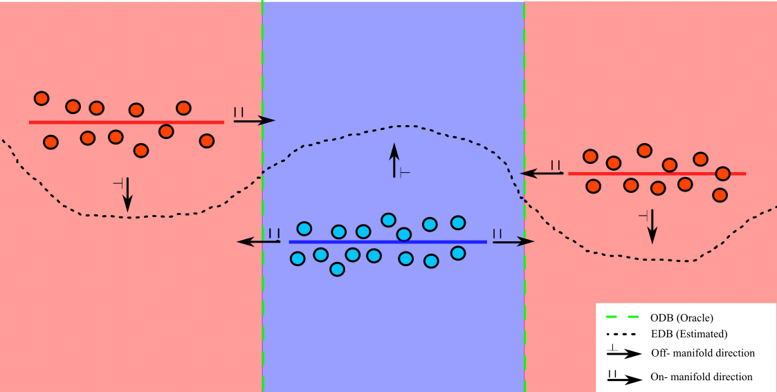
Figure 1: Mental image: The oracle decision boundary (green dashed line) determines the label (blue or red) of any point in the Euclidean space. The observed data space consists of 1-dimensional line segments immersed in the 2-dimensional space. The model learns the estimated decision boundary (black dotted line) based on the observed data.

For a classification problem, assume that there exists an oracle decision boundary (ODB), which is the human decision boundary that determines the labels for any lawful input (e.g., a consensus digit recognition rule for any arbitrary gray-level images). The goal of training a neural network classifier is to obtain an estimated decision boundary (EDB) based on observed data (sample-label pairs observed). To facilitate misclassification by the neural network, a perturbation must push the original sample across the EDB.

Different types of attacks can be defined when the data is only observable in a particular subspace of the lawful input space (the data space). Usually, the EDB can estimate the ODB within the data space reasonably, given a large sample size. Thus, an adversarial perturbation restricted to the data space, which aims to cross over the ODB, tends to cross over the EDB as well. We call these adversarial attacks natural or on-manifold attacks. Even an oracle will be prone to wrong classifications with these adversarial perturbations.

In contrast, outside the data space, where no observation is made, the EDB curve is merely an extrapolation extended from the data space. It will not necessarily approximate the ODB well. Consequently, an adversarial perturbation outward from the data space, facilitated by crossing the EDB, will not necessarily try to push the sample over the ODB. We call these perturbations unnatural or off-manifold attacks. Under these attacks, an oracle can accurately distinguish and classify the perturbed sample, but the trained model fails. Figure 1 is provided to illustrate this phenomenon with a simple example. Shamir et al. (2022)’s observations also support the phenomenon we describe, where the EDB learned by neural networks, over the training process, tends to align with the data space first and then form dimples around differently labeled clusters to attain correct classification on the observed data space, leaving them vulnerable to examples outside the data space.

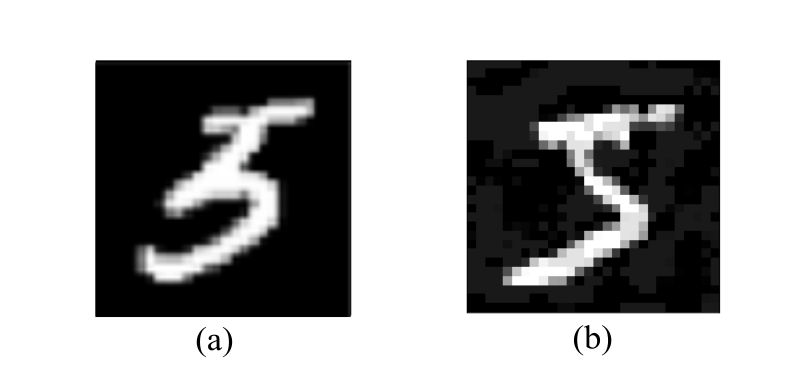
Figure 2: Original image is a digit 5. (a) Natural attack; (b) Unnatural attack (minor changes in pixel values of the background compared to the original). Under both of these attacks, the neural network classifies the image as 3 instead of 5.

Figure 2 shows an example of an unnatural and natural attack on a digit 5 image in the MNIST dataset (LeCun et al., 2010). The unnatural attacked image can still be classified as 5 by a human/oracle; however, the model classifies it as digit 3. The vulnerability of neural networks to unnatural attacks is a pressing issue.

In this work, we obtain distinguished results for off-manifold and on-manifold attacks. Our results imply that unnatural/off-manifold attacks are fundamental consequences of the dimension gap between the local intrinsic dimension of the observed data space and the ambient dimension. That is,

Theorem 1.1 (Informal version of Theorem 4.2).

As the dimension gap increases, the strength of $\ell_{2},\ell_{\infty}$ attack required to misclassify the sample decreases, i.e., the model is more vulnerable. Notably, for $\ell_{\infty}$ attack, the strength asymptotically goes to $0$ w.r.t. the dimension gap.

We use intrinsic dimension as an umbrella term for well-known concepts of Manifold dimension, Minkowski dimension, Hausdorff dimension etc. In our theoretical setting (Section 3.1), all of these notions of dimension are equivalent and refer to the signal residing in a lower dimensional set locally.

	Ambient	LPCA	MLE(k=5)	TwoNN
MNIST	784	38	13.36	14.90
CIFAR-10	3072	9	27.66	31.65

Table 1: Intrinsic dimension estimation

To fuel the reader’s motivation, Table 1 is presented to show the estimated local intrinsic dimension for the standard image datasets MNIST and CIFAR-10. Regardless of the estimation method (local PCA(Fukunaga and Olsen, 1971), maximum likelihood estimation(Haro et al., 2008), Two nearest-neighbor(Facco et al., 2017)), the ambient dimension of the images is way larger than the intrinsic dimension of the space they reside in. This paper reveals that this is the root cause of the existence of unnatural attacks. Furthermore, as implied by our theorem, a larger ambient-intrinsic dimension gap, e.g., training images with unnecessarily high resolution but no more useful details, leads to higher vulnerability.

2 Related Works

Besides the literature, as mentioned earlier, below is a list of works ordered by relatability to this paper.

Adversarial study motivated by a manifold view

(Xiao et al., 2022) assumes a manifold view of the data and focuses on a generative model to learn the data manifold and conceive on-manifold attacks in practice. (Zhang et al., 2022) conducts a theoretical study to decompose the adversarial risk into four geometric components: the standard risk, nearest neighbor risk, in-manifold, and normal (off-manifold in our setting) risk. Our paper also subscribes to the manifold hypothesis; Compared to the above two studies, our focus and mathematical setting are on the relationship between the data dimension gap and adversarial attack strength.

Adversarial examples in random ReLU networks

Different from this paper which studies trained neural networks, some other studies, e.g., Daniely and Shacham (2020); Bubeck et al. (2021) also show the existence of $\ell_{2}$ adversarial examples in two-layer ReLU networks with randomized weights and provide a corresponding rate for the strength of the $\ell_{2}$ perturbation. Bartlett et al. (2021) further generalizes to a multi-layer network.

Adversarial examples due to implicit bias in two-layer Relu networks

Vardi et al. (2022) and Frei et al. (2023) argue that adversarial examples are a consequence of the implicit bias in clean training despite the existence of robust networks. Extending from their work, we introduce the notion of the intrinsic-ambient dimension gap exhibited by the data, which gives rise to two different types of attacks natural or on-manifold and unnatural or off-manifold. The previously mentioned works can be reduced to the on-manifold setting in our framework.

Adversarial examples due to low dimensional data

A recent work, Melamed et al. (2023), studies the adversarial robustness of clean-trained neural networks with data in a low-dimensional linear subspace and argues that the neural networks are vulnerable to attacks in the orthogonal direction.

Though the motivation is similar, our findings and outcomes are different. Detailed comparisons of are provided in Section 3.5 for the model setup, and Section 4 for the final result, respectively. In short, the key differences arise from their setting of linear subspace, lazy training, and weight initialization. Though it is worth consideration in the finite training regime, the adversarial vulnerability considered in their setting does not hold if the neural network training attains convergence. On the other hand, our results are invariant to initialization, and our theoretical setting is more realistic than prior works.

3 Problem Setup

In this section, we introduce the detailed technical settings considered in this paper. We use consistent notations with Frei et al. (2023) in this paper. For any natural number $n$, the set $\{1,\ldots,n\}$ is represented by the shorthand $[n]$. For any vector $\mathbf{u}$, $\left\|\mathbf{u}\right\|$ will denote the euclidean $\ell_{2}$ norm. The notations ${\cal O}{}$ and $\Theta$ are the standard asymptotic notations.

3.1 Data

In this paper, we study a binary classification problem with $k$ clusters with respective labels $y^{(r)}\in\{-1,1\},\,r\in[k]$ and $n$ observations. The intrinsic signal lies in $d$ dimensions, and we observe some transformation of the signal in $D$ dimensions ($D\geq d$). The dimension gap is denoted by $g=D-d$. Let $\mathbf{x}_{i}=\bm{\mu}^{(r)}+\bm{\xi}_{i}\in\mathbb{R}^{d}$ denote the $i^{th},\,i\in[n]$ intrinsic signal for the $r^{th}$ cluster. The vectors $\bm{\mu}^{(1)},\ldots,\bm{\mu}^{(k)}\in\mathbb{R}^{d}$ are the means of the $k$ clusters, and $\bm{\xi}_{i}\in\mathbb{R}^{d}$ is the deviation of the signal around the mean.

In terms of the actual observed data, denote the $i^{th}$ observation $\tilde{\mathbf{x}}_{i}=\mathbf{M}\mathbf{x}_{i}+\bm{\zeta}^{(r)}+\bm{\omega}_{i}\in\mathbb{R}^{D}$, where $\mathbf{M}$ is a $D\times d$ matrix with $d$- orthonormal columns; the vector $\bm{\zeta}^{(r)}\in\mathbb{R}^{D}$ is the additional random cluster effect and $\bm{\zeta}^{(r)}\sim N(0,\tau^{2}\mathbf{I}_{D})$ for all $r\in[k]$; and $\bm{\omega}_{i}$ represents the ambient noise. We will also use an alternate representation for the $i^{th}$ observation in terms of the transformed mean and deviation term in higher dimensions, $\tilde{\mathbf{x}}_{i}=\tilde{\bm{\mu}}^{(r)}+\tilde{\bm{\xi}}_{i}$ where $\tilde{\bm{\mu}}^{(r)}=\mathbf{M}\bm{\mu}^{(r)}$ and $\tilde{\bm{\xi}}=\mathbf{M}\bm{\xi}_{i}+\bm{\zeta}^{(r)}+\bm{\omega}_{i}$. The terms $\bm{\xi}_{i},\bm{\omega}_{i}$ are also random, and we do not impose any specific distribution for them; instead, we will restrict their norm for our analysis. The notation ${\cal S}=\{(\tilde{\mathbf{x}}_{i},y_{i})\}_{i=1}^{n}$ is the collection of all $n$ observation-label pairs used to train our model.

3.2 Data Interpretation

When studying low-dimensional information embedded in a higher-dimensional space, we do not want the original information to be lost or distorted. We restrict our analysis to a class of transformations known as Isometric Transformations. Isometric transformations are essential as they preserve distances (structure/information) between any pair of points in the origin space.

Any isometric transformation can be expressed as an affine transformation with a linear part consisting of orthogonal columns and a geometric translation. Hence, $\mathbf{M}(\cdot)+\bm{\zeta}^{(r)}$ preserves distance within each cluster. The matrix $\mathbf{M}$ applies a linear transformation on the $d$-dimensional intrinsic signal ($\mathbf{x}_{i}$), immersing it into a $D$-dimensional space. After the immersion, a translation or shift $\bm{\zeta}^{(r)}$ is added corresponding to the $r^{th}$ cluster. Then an ambient noise $\bm{\omega}$ is added to account for the stochasticity in the observation process. Each cluster can be considered a lower $d$ dimensional manifold immersed in a $D$ dimensional space up to ambient noise. Our data space is a union of such manifolds, and our setup can be used as a motivation for real-life datasets that locally reside in a lower dimensional manifold. Examples can be found in Tables 1, 2, 4, 5.

CIFAR class	0	1	$\dots$	8	9
LPCA	8	11	$\dots$	10	16
MLE (k=5)	18.34	21.20	$\dots$	19.80	24.42
TwoNN	21.77	25.98	$\dots$	24.77	29.11

Table 2: Intrinsic dimension of CIFAR-10 Dataset. The intrinsic dimension over all classes is similar to that for individual classes. (Complete version: Table 4 in the appendix.)

Within each cluster $r$, the distances are preserved by the transformation $\mathbf{M}(\cdot)+\bm{\zeta}^{(r)}$ up to the variance introduced by the ambient noise ($Var(\bm{\omega})$). Between clusters, the distances are preserved by $\mathbf{M}(\cdot)$ up to a slightly larger variance due to cluster translation and the noise term $(2\tau^{2}+Var(\bm{\omega}))$. Intuitively, our setup transforms a low-dimensional signal into a high-dimensional signal via $\mathbf{M}$, preserving all information (pairwise angle and distances) up to some variance, where the within-cluster variance is lower than the between-cluster variance.

3.3 Neural Network

In this work, we will use a 2-layer ReLU network ${\cal N}_{{\bm{\theta}}}:\mathbb{R}^{D}\to\mathbb{R}$ of width $w$ as our classification model.

$${\cal N}_{{\bm{\theta}}}(\tilde{\mathbf{x}})=\sum_{j=1}^{w}v_{j}\phi(\mathbf{w}_{j}^{\top}\tilde{\mathbf{x}}+b_{j})$$ (1)

$\mathbf{w},b$ represent the weights and biases of the first layer; $v_{j}$ is a scalar weight of the second layer for the $j^{th}$ neuron. The function $\phi(x)=\max(0,x)$ is the ReLU activation function. The vectorized collection of all the parameters $(\mathbf{w}_{1}^{T},\ldots,\mathbf{w}_{j}^{T},b_{1}\ldots,b_{j},v_{1},\ldots,v_{j})^{T}$ for the neural network is represented by ${\bm{\theta}}$. Both the two layers will be updated during the training.

3.4 Expression for Network Parameters

Before we proceed, we need to establish the training loss used in our framework. For our neural network model ${\cal N}_{{\bm{\theta}}}$ parameterized by ${\bm{\theta}}$, the empirical loss ${\cal L}({{\bm{\theta}}})$ can be defined on the dataset ${\cal S}=\{(\tilde{\mathbf{x}}_{i},y_{i})\}_{i=1}^{n}$ as follows:

$${\cal L}({\bm{\theta}}):=\frac{1}{n}\sum_{i=1}^{n}\ell(y_{i}\cdot{\cal N}_{{\bm{\theta}}}(\tilde{\mathbf{x}}_{i}))~{}.$$ (2)

When $\ell(z)=e^{-z}$ or $\ell(z)=\log(1+e^{-z})$, ${\cal L}({\bm{\theta}})$ is the empirical exponential loss or logistic loss respectively.

Some implicit bias literature studies the limiting behavior of the training process. Based on Lyu and Li (2020), two-layer ReLU networks have directional convergence to the solution of the maximum margin problem (James et al., 2013):

Theorem 3.1 (Lyu and Li (2020)).

Consider ${\cal N}_{\theta}(\tilde{\mathbf{x}})$ trained via gradient descent or gradient flow for the exponential or logistic loss. If for some time $t_{0}$ in the training process, the loss reaches a sufficiently small value ${\cal L}(\theta(t_{0}))<\frac{1}{n}$. Then, under some regularity and smoothness assumptions, $\frac{{\bm{\theta}}}{\|{\bm{\theta}}\|}$converges to the KKT solution of the maximum margin problem:

$$\min_{\bm{\theta}}\frac{1}{2}\left\|{\bm{\theta}}\right\|^{2}\;\;\;\;\text{s.t. }\;\;\;\forall i\in[n]\;\;y_{i}{\cal N}_{{\bm{\theta}}}(\tilde{\mathbf{x}}_{i})\geq 1~{}.$$ (3)

Furthermore, ${\cal L}({\bm{\theta}}(t))\to 0$ and $\left\|{\bm{\theta}}(t)\right\|\to\infty$ as $t\to\infty$.

Theorem 3.1 shows the limiting behavior of the gradient flow in clean training and generally applies to any homogeneous network defined in Lyu and Li (2020). A consequence of the above theorem is that we can express the parameters in terms of the data, i.e., ${\bm{\theta}}=\sum_{i}^{n}\lambda_{i}y_{i}\nabla_{{\bm{\theta}}}{\cal N}_{{\bm{\theta}}}(\tilde{\mathbf{x}}_{i})$, where $\lambda_{i}\geq 0$ are the Lagrangian multipliers. Specifically,

$$\mathbf{w}_{j}=\sum_{i\in[n]}v_{j}\lambda_{i}y_{i}\phi^{\prime}_{i,j}\tilde{\mathbf{x}}_{i};\hskip 8.5359ptb_{j}=\sum_{i\in[n]}v_{j}\lambda_{i}y_{i}\phi^{\prime}_{i,j}$$ (4)

$\phi^{\prime}_{i,j}$ denotes the sub gradient of $\phi(\mathbf{w}_{j}^{\top}\tilde{\mathbf{x}}_{i}+b_{j})$.

3.5 Volatile biases

In the previous section, we saw that the network parameters can be explicitly written in terms of the observed dataset. In this section, we will leverage that closed-form expression to justify the existence of vulnerable weight components responsible for unnatural attacks.

Let $\mathbf{P}_{o}=\mathbf{M}(\mathbf{M}^{\top}\mathbf{M})^{-1}\mathbf{M}^{\top}=\mathbf{M}\mathbf{M}^{\top}$ be the projection matrix of the image space where the intrinsic signal is initially immersed. On the contrary, $\mathbf{P}=\mathbf{I}_{D}-\mathbf{P}_{o}$ is the projection onto the co-kernel, where no component of the intrinsic signal $\mathbf{x}$ resides. We will associate the terms on-manifold and off-manifold to the spaces dictated by $\mathbf{P}_{o}$ and $\mathbf{P}$, respectively.

In the neural network, each weight $\mathbf{w}_{j}$ can be decomposed into an authentic-weights part $\mathbf{P}_{o}\mathbf{w}_{j}$ and a volatile biases part $\mathbf{P}\mathbf{w}_{j}$. Multiplying, $\mathbf{P}_{o},\mathbf{P}$ to Eq. (4) we get:

$$\mathbf{P}_{o}\mathbf{w}_{j} =\sum_{i\in[n]}\lambda_{i}y_{i}v_{j}\phi^{\prime}_{i,j}\left[\mathbf{M}\mathbf{x}_{i}+\mathbf{P}_{o}\left(\bm{\zeta}^{(r)}+\bm{\omega}_{i}\right)\right]$$

$$\mathbf{P}\mathbf{w}_{j} =\sum_{i\in I^{(r)}}\sum_{r\in[k]}\lambda_{i}y_{i}v_{j}\phi^{\prime}_{i,j}\mathbf{P}\left(\bm{\zeta}^{(r)}+\bm{\omega}_{i}\right),$$ (5)

where $I^{(r)}$ is the index set of samples in the $r^{th}$ cluster. The authentic weights are the ones that carry all the information of the intrinsic signal $\mathbf{x}$ from the lower $d$ dimension space; the volatile biases are dummy weights (independent of $\mathbf{x}$) that act just as additional bias terms during the clean training. Any interaction between the immersed intrinsic signal and volatile biases is zero as $\mathbf{P}\mathbf{M}=0$. However, they can be exploited by off-manifold attacks to change the neuron output.

Comparison to Melamed et al. (2023)

In Melamed et al. (2023), the setting is equivalent to a linear transformation of a low-dimensional intrinsic signal to a higher dimension, i.e., under our framework, $\tilde{\mathbf{x}}=\mathbf{L}\mathbf{x}$ where $\mathbf{L}$ is any $D\times d$ matrix. Let $\pi^{\perp}=\mathbf{I}_{D}-\mathbf{L}(\mathbf{L}^{\top}\mathbf{L})^{-1}\mathbf{L}^{\top}$ be the projection matrix. Using Theorem 3.1 and Eq. (4) in their setting, we have $\pi^{\perp}\mathbf{w}_{j}=0\,,j\in[w]$.

The consequence is that, based on results in Theorem 3.1, at convergence, the orthogonal weights converge to 0; hence, these weights have no contribution to the neuron output. The adversarial vulnerability described in Melamed et al. (2023) results from finite training and large weight initialization. In real practice, since one can only train finite iterations, the initialization property observed by Melamed et al. (2023) is still a factor to consider. However, it is not the driving force for the existence of unnatural attacks. We also validate these arguments with experiments on simulated and real-life datasets (Section 5.1).

3.6 Assumptions

In this section, we introduce some additional assumptions to simplify the analysis.

Assumption 3.2.

We have:

1. $\left\|\bm{\mu}^{(j)}\right\|=\sqrt{d}$ for all $r\in[k]$.

2. $k\left(\max_{i\neq j}|\langle\bm{\mu}^{(i)},\bm{\mu}^{(j)}\rangle|+\Delta^{\prime}+1\right)=c^{\prime}(d-\Delta^{\prime}+1)$. ; $c^{\prime}<1/10$

3. $\left\|\bm{\xi}\right\|\leq\sqrt{2}\ln(d);\left\|\bm{\omega}\right\|\leq 1$

4. $c_{3}(g,\tau,k)=\frac{g\tau^{2}}{20k}-\frac{10k+1}{10k}\sqrt{\frac{13g\tau^{2}}{8}}>0;$
   $c_{5}(d,\tau,k)=\frac{d\tau^{2}}{20k}-\frac{10k+1}{10k}\sqrt{\frac{13d\tau^{2}}{8}}(\sqrt{2\ln d+1})\\ >0;$

where $\Delta^{\prime}={\cal O}{\left(\max\{\sqrt{d}\ln d,D\tau^{2}\}\right)}$ (Definition B.2).

Assumptions $(A1),(A2)$ are similar to the assumptions used in Frei et al. (2023). Condition $(A1)$ states that the signal strength must grow with the intrinsic dimension. It can be generalized by replacing $\sqrt{d}$ to $\Theta{(\sqrt{d})}$ without changing the analysis in any meaningful way. Condition $(A2)$ ensures that the means are near orthogonal to each other; we impose that pairwise interaction between the means is less than $\left\|\bm{\mu}^{(r)}\right\|^{2}=d$ for any cluster $r$. This assumption can be satisfied for some $\tau^{2}={\cal O}{(d/D)}$.

For the other two assumptions, $(A3)$ are bounds on the stochastic deviation and error terms. In general, these bounds can be relaxed to ${\cal O}{(\ln d)},{\cal O}{(1)}$ respectively. These bounds are easy to satisfy for sufficiently large $d$, for instance, $\bm{\xi}\sim N(0,\mathbf{I}_{d});\bm{\omega}\sim N(0,D^{-1}\mathbf{I}_{D})$ satisfy the above bounds with high probability. In addition, Condition $(A4)$ is a mild assumption. The order of the positive terms is higher than the negative terms for both $c_{3}(g,\tau,k)$ and $c_{5}(d,\tau,k)$. A constant can always be incorporated inside $\tau$ to satisfy the assumption.

4 Main Results

In this section, we will state our main results. We study the adversarial vulnerability for any reasonable testing samples that arise from the observable data space (union of manifolds) and are homogeneous with training samples. Formally, we define such examples as nice examples 4.1. These examples can be expressed as the transformation of some $d$ dimensional intrinsic signal described in Section 3.1.

Definition 4.1 (Nice example).

An $\tilde{\mathbf{x}}\in\mathbb{R}^{D}$ is nice if it can be expressed as $\tilde{\mathbf{x}}=\mathbf{M}\mathbf{x}+\bm{\zeta}^{(r)}+\bm{\omega}$, for some $r\in[k]$ and $\mathbf{x}=\bm{\mu}^{(r)}+\bm{\xi}$ such that $\left\|\bm{\xi}\right\|\leq\sqrt{2}\ln(d)$, $\left\|\bm{\omega}\right\|\leq 1$.

In the following theorem, we show that for any nice-example, the clean-trained neural network accurately predicts the labels.

Theorem 4.1.

Suppose ${\cal S}$ satisfies the assumption 3.2 and clean training has attained convergence under the setting of Theorem 3.1. Let $\tilde{\mathbf{x}}\in{\mathbb{R}}^{D}$ and $r\in[k]$ such that $\tilde{\mathbf{x}}$ is a “nice example” (Definition 4.1). Then with probability $1-2\exp(-\frac{D}{16})$, $\operatorname*{sign}\left({\cal N}_{{\bm{\theta}}}(\tilde{\mathbf{x}})\right)=y^{(r)}$.

Theorem 4.1 states that the trained neural network can generalize well with a high probability when we have an example from the low-dimensional data space. Asymptotically, as the ambient dimension $(D\to\infty)$ increases, this probability converges to 1.

However, even if the clean training generalizes well, our following theorem states that for any nice example $\tilde{\mathbf{x}}$, there exists perturbation $\mathbf{z}_{\shortparallel}$ and $\mathbf{z}_{\perp}$ in the on-manifold and off-manifold direction which successfully misclassify the model with high probability.

Theorem 4.2.

Suppose ${\cal S}$ satisfies Assumption 3.2 and clean training has attained convergence under the setting of Theorem 3.1. Let $\tilde{\mathbf{x}}\in{\mathbb{R}}^{D}$ and $r\in[k]$ such that $\tilde{\mathbf{x}}$ is a “nice example” (Definition 4.1). Then there exist perturbations $\mathbf{z}_{\perp}\propto\mathbf{u}_{\perp},\,\mathbf{z}_{\shortparallel}\propto\mathbf{u}_{\shortparallel}$ with probability at least $1-\delta_{1},1-\delta_{2}$ respectively; Such that, ${\cal N}_{\bm{\theta}}(\tilde{\mathbf{x}}-\mathbf{z}_{\perp}),\,{\cal N}_{\bm{\theta}}(\tilde{\mathbf{x}}-\mathbf{z}_{\shortparallel})\leq-1$ for $r\in Q_{+}$ and ${\cal N}_{\bm{\theta}}(\tilde{\mathbf{x}}+\mathbf{z}_{\perp}),\,{\cal N}_{\bm{\theta}}(\tilde{\mathbf{x}}+\mathbf{z}_{\shortparallel})\geq 1$ for $r\in Q_{-}$. Also,

$$\left\|\mathbf{z}_{\perp}\right\|={\cal O}{\left(\frac{d}{c\sqrt{kg\tau^{2}}}\right)},\left\|\mathbf{z}_{\perp}\right\|_{\infty}={\cal O}{\left(\frac{d\sqrt{2\log(2g)}}{cg\tau}\right)},$$

$$\left\|\mathbf{z}_{\shortparallel}\right\|={\cal O}{\left(\sqrt{\frac{d}{c^{2}k(2+\tau^{2})}}\right)},$$

$$\left\|\mathbf{z}_{\shortparallel}\right\|_{\infty}={\cal O}{\left(\frac{\sqrt{d}+\tau\sqrt{2\log(2d)}}{c(2+\tau^{2})}\right)},$$

where $\mathbf{u}_{\shortparallel}=\sum_{q\in[k]}y^{(q)}\left(\tilde{\bm{\mu}}^{(q)}+\mathbf{P}_{o}\bm{\zeta}^{(q)}\right)$ and $\mathbf{u}_{\perp}=\sum_{q\in[k]}y^{(q)}\mathbf{P}\bm{\zeta}^{(q)}$. $Q_{+},Q_{-}$ are a set of clusters with labels $1,-1$ respectively and $c=k^{-1}\min\{|Q_{+}|,|Q_{-}|\}$. Probabilities $\delta_{1},\delta_{2}$ are defined in Lemmas C.1.5, C.1.7 respectively.

Theorem 4.2 provides an upper bound on the strength of an on-manifold ($\mathbf{z}_{\shortparallel}$) and off-manifold ($\mathbf{z}_{\perp}$) adversarial perturbation for any nice example. These upper bounds hold with probability $1-\delta_{1},1-\delta_{2}$ for on/off-manifold perturbations respectively, where $\delta_{1}\to 0$ as $D\to\infty$ and $\delta_{2}\to 0$ as $D,d\to\infty$.
Note that $\tau^{2}={\cal O}{(d/D)}$ based on our assumptions (Section 3.6), hence we see that $\ell_{2}$ strength of $\mathbf{z}_{\perp}$ decreases as the dimension gap $g$ increases and asymptotically (in $g$) is equivalent to ${\cal O}{(d/(c\sqrt{k}))}$. For $\mathbf{z}_{\shortparallel}$ the $\ell_{2}$ strength increases and saturates to ${\cal O}{(\sqrt{d/(c^{2}k)})}$ as $g\to\infty$.

On the other hand, the $\ell_{\infty}$ strength of $\mathbf{z}_{\perp}$ and $\mathbf{z}_{\shortparallel}$ goes to $0$ and ${\cal O}{(\sqrt{d})}$, respectively as $g\to\infty$. That is, asymptotically, the $\ell_{2}$ strength of on-manifold is a bit smaller (or comparable ) than the off-manifold perturbation, but in contrast the $\ell_{\infty}$ strength for the off-manifold perturbation goes to 0 while the on-manifold perturbation is still some constant depending on $d$. Additionally, the asymptotic upper bound for on-manifold perturbation reduces to the rate to Frei et al. (2023); our framework is an extension introducing dimension gap and two distinct attack spaces, Frei et al. (2023) results can be related to our on-manifold perturbation results. As these are upper-bound results to an existential result, they also act as an upper bound to the smallest adversarial perturbation. In Section 5, we will validate the tightness of these upper bounds with empirical experiments.

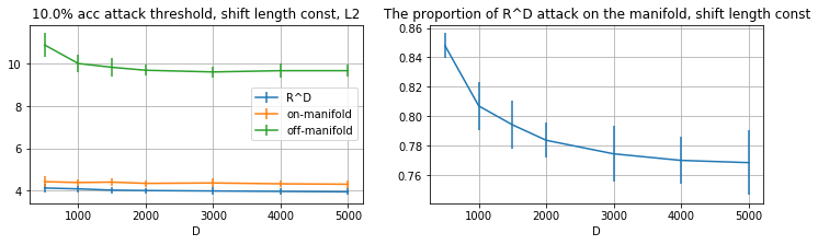
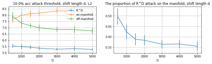
Figure 3: Attack strength threshold associating with $10\%$ robust test accuracy (left) and the on-manifold proportion in $\mathbb{R}^{D}$ attack. The top and bottom rows correspond to the cases $\|\bm{\zeta}\|=\Theta(1),\Theta(\sqrt{d})$ respectively.

Rate comparison with Melamed et al. (2023)

Despite the differences in Melamed et al. (2023) and our theoretical setting ( Remark 3.5), we can attempt to draw some parallels with their main result. In Melamed et al. (2023), an adversarial perturbation (off-manifold) exists as a function of orthogonal weights when an observation $\tilde{\mathbf{x}}$ strictly resides in a $d$ dimensional linear subspace of a $D$ dimensional Euclidean space (dimension gap $g=D-d$). The $\ell_{2}$ strength of this off-manifold perturbation in our notation can be expressed as ${\cal O}{\left(N(\tilde{\mathbf{x}})\sqrt{\frac{D}{g}}\right)}$ up to some constants. Here, $N(\cdot)$ represents their two-layer ReLU lazy-trained network. For the case when $\tau^{2}=\Theta\left(\frac{d}{D}\right)$ in Theorem 4.2, we can obtain a similar rate for $\|\mathbf{z}_{\perp}\|$ in our framework. However, for smaller $\tau^{2}$, the rate in our result is smaller.

5 Experiments

In this section, we conduct a simulation study and experiments in the MNIST dataset to exhibit that the data dimension plays an essential role in adversarial robustness. Due to the page limit, we postpone some figures to the appendix.

5.1 Simulation Study

To generate the data, we first generate $k$ means $\{\bm{\mu}^{(r)}\}_{r=1}^{k}$ corresponding to the $k$ clusters in the lower $d$ dimension from $\bm{\mu}^{(r)}\sim N(0,\mathbf{I}_{d})$. This enforces that $\|\bm{\mu}^{(r)}\|=\Theta(d)$ with high probability, which is a relaxed version of assumption (A1). Given the $k$ cluster means, we generate $n=1000$ intrinsic data signals $\{\mathbf{x}_{i}\}_{i=1}^{1000}$ centered around these means drawn uniformly. For each $i$, $\mathbf{x}_{i}=\bm{\mu}_{i}+\bm{\xi}_{i}$, where $\bm{\mu}_{i}\sim\mathcal{U}(\bm{\mu}^{(1)},\ldots,\bm{\mu}^{(k)})$ and $\bm{\xi}_{i}\sim N(0,\mathbf{I}_{d}/d)$, which enforces assumption (A3) with high probability.

After getting the intrinsic data signals $\{\mathbf{x}_{i}\}_{i=1}^{1000}$, we immerse them into a $D(\gg d)$ dimension space to get our observed data samples $\{\tilde{\mathbf{x}}_{i}\}_{i=1}^{1000}$. In alignment with our theoretical setting, we apply a matrix $\mathbf{M}$ for the initial linear transformation. We emulate this matrix by generating $d$, $D$-dimensional $N(0,D^{-1}\mathbf{I}_{D})$ Gaussian vectors $m_{1},\ldots,m_{d}$; which act as the column of $\mathbf{M}$. This is justified as when $D\gg d$ and $i\neq j$, $m_{i}^{\top}m_{j}=O_{p}(1/\sqrt{D})$, i.e., the $d$ vectors are almost orthogonal. Lastly, we add translations $\{\bm{\zeta}^{(r)}\}_{r=1}^{k}$ corresponding to each cluster. We generate $\bm{\zeta}^{(r)}\sim N(0,\tau^{2}\mathbf{I}_{D})$ for each cluster $r=1,\ldots,k$, the choice of $\tau^{2}=D^{-1},dD^{-1}$ corresponds to $\|\bm{\zeta}^{(r)}\|=\Theta(1),\Theta(\sqrt{d})$ respectively, with high probability. The architecture and training details can be found in Appendix D.1.1.

To validate our theory, we need to find the minimal attack strength required to misclassify an example. This is not computationally feasible; hence as an alternative, we find the minimal attack strength required to misclassify a large proportion of the data. We iterate over attack strengths until reaching 10% robust testing accuracy. The details are in Appendix D.1.2.

In the first simulation, we fix the intrinsic dimension $d=100$ and vary the ambient dimension $D$. The results are summarized in Figure 3. The top panel of Figure 3 is the $\ell_{2}$ attack strength for $\mathbb{R}^{D}$, on-manifold, and off-manifold attacks. The bottom panel is the proportion of $\mathbb{R}^{D}$ attack that lies on the manifold. The rows of Figure 3 corresponds to the cases when $\|\bm{\zeta}^{(r)}\|$ is $\Theta(\sqrt{d})$ and $\Theta(1)$ or $\tau^{2}=dD^{-1},D^{-1}$ respectively.

There are two observations. First, the trends for $\ell_{2}$ attack strength in Figure 3 are as expected as in the discussion in Theorem 4.2.

Second, the bottom panel of the figure shows the ratio of the on-manifold component to the off-manifold component for the $\mathbb{R}^{D}$ attack. We see that as $D$ increases, this proportion decreases, implying that even when the attack has no constraint with an increase in $D$ or $g$, the model becomes more vulnerable to off-manifold perturbations.

Figure 9 in the appendix is analogous to Figure 3 but considering the $\ell_{\infty}$ norm of the attack. The observations are consistent with the discussion succeeding Theorem 4.2. One difference is that for $\ell_{\infty}$ upper bound of the on-manifold attack, it also approaches $0$ instead of a constant (in $D,g$) ${\cal O}{(\sqrt{d})}$. This is an artifact of generating $\mathbf{M}$ from random Gaussian vectors instead of the fixed-$\mathbf{M}$ scenario considered in Theorem 4.2.

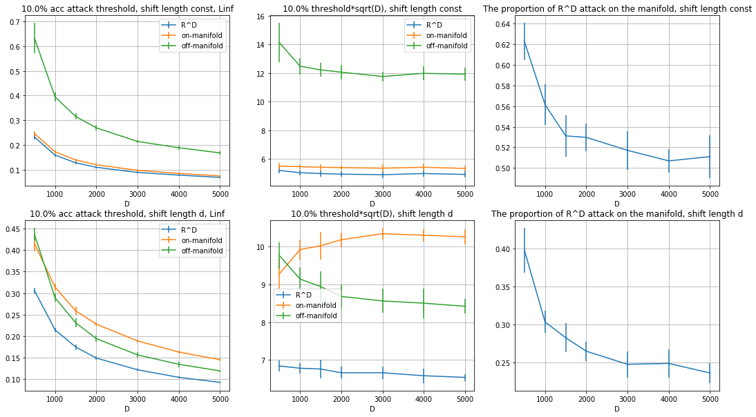
Figure 10: Attack strength threshold associating with $10\%$ robust test accuracy (left), its scaled value (middle), and the on-manifold proportion in $\mathbb{R}^{D}$ attack. The top and bottom rows correspond to the cases $\|\bm{\zeta}\|=\Theta(1),\Theta(\sqrt{d})$ respectively.

In the appendix, we also plot the attack threshold generated by $\ell_{\infty}$ attacks. The results are provided in Figure 10. They are identical to the results of Figure 9, implying our bounds provide accurate guidance for the $\ell_{\infty}$ case. Intuitively, when $D$ increases, the total attack budget grows when fixing the $\ell_{\infty}$ attack strength, so we observe a decreasing trend in the top panel of Figure 10. Besides, if we multiply the attack strength by $\sqrt{D}$, we can observe a similar trend as the $\ell_{2}$ attack in Figure 3, consistent with our prior discussions.

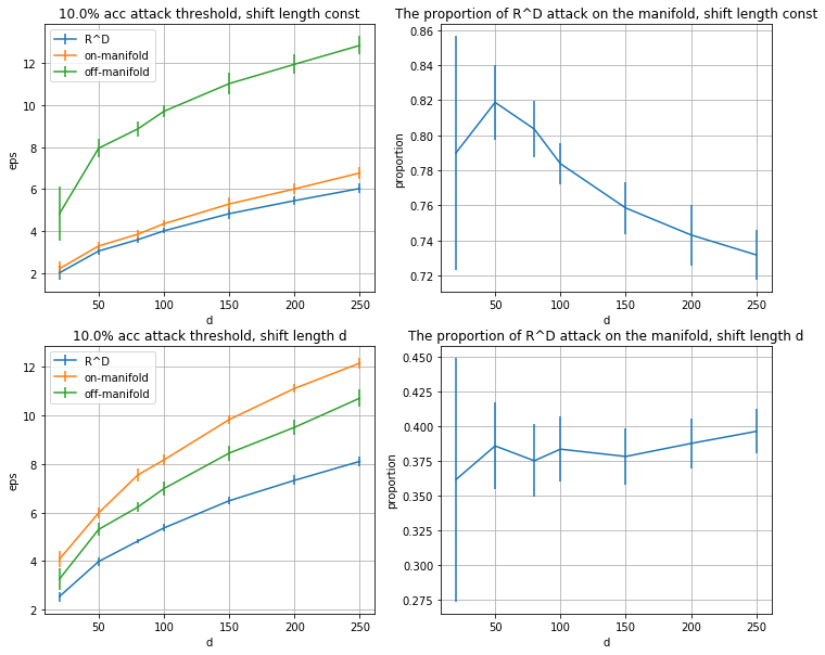
Figure 11: Attack strength threshold associating with $10\%$ robust test accuracy (left) and the on-manifold proportion in $\mathbb{R}^{D}$ attack when changing $d$. The top and bottom rows correspond to the cases $\|\bm{\zeta}\|=\Theta(1),\Theta(\sqrt{d})$ respectively.

In contrast to the first simulation, we fix the ambient dimension $D=2000$ in the second simulation and vary the intrinsic dimension $d$. We track the attack threshold as a function of $d$. The results are provided in the appendix, Figure 11. One can see that when $d$ increases, there is more on-manifold information; thus, the model is more robust.

Effect of Initialization

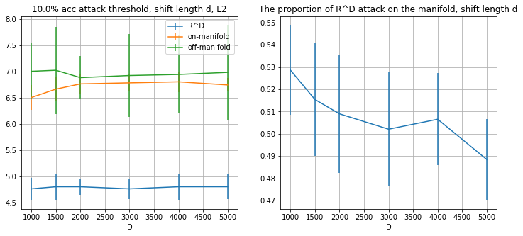
Figure 12: Attack strength threshold associating with $10\%$ robust test accuracy (left) and the on-manifold proportion in $\mathbb{R}^{D}$ attack when changing $d$. The initialization in this setting is 0.01 of the initialization used in all other figures.

We also conduct experiments to examine the effect of neural network initialization and $\ell_{2}$ regularization (weight decay). In the appendix, the results are postponed to Figure 12 and 13. The trained model slightly improves when using a small initialization or weight decay compared to Figure 3. However, the vulnerability towards off-manifold attack in these two scenarios is similar to Figure 3. That is, dimension-gap hampers robustness regardless of the initialization.

5.2 MNIST Dataset

We also conduct experiments on the MNIST dataset to validate the effect of the gap between intrinsic and ambient dimensions on the adversarial robustness. According to our theoretical setup, the MNIST dataset can be considered as a union of low-dimensional local clusters immersed in a high-dimensional space as bolstered by Table 5 in the appendix.

Different from the simulation, we cannot access the low-dimensional intrinsic signal corresponding to the MNIST images; the original data set already has some dimension gap. Regardless, we can still attempt to track the effect of the additional dimension gap on the adversarial robustness. To make a fair assessment, we implement isometric transformations on the original MNIST images that increase the ambient dimension $D$ to track the dependence of attack strength with varying dimensions.

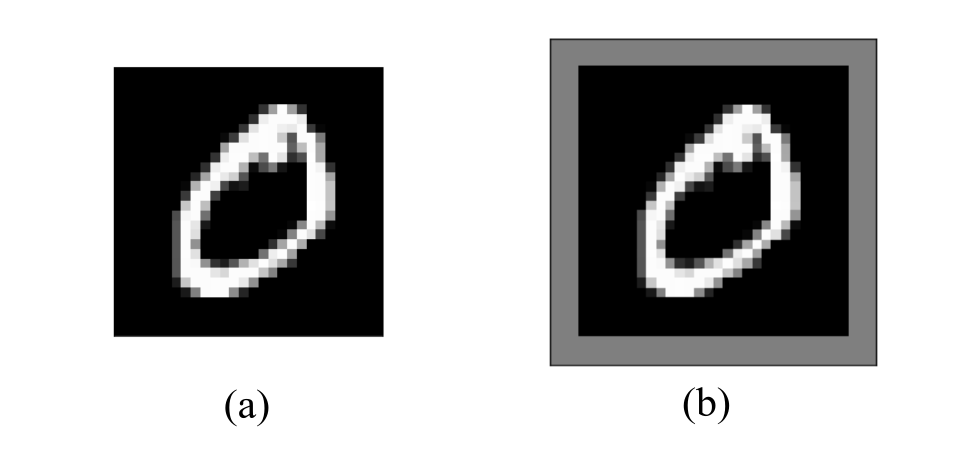
Figure 4: (a) Original image 28x28, $D=784$; (b) Padded image 34x34, $P=3$, $D=1156$.

We pad gray (0.5) pixels on the image’s border to increase the ambient dimension (Figure 4). Adding a pad of $P$ pixels along the borders increases the ambient dimension $D$ by $4P^{2}+2P$. Adding gray borders to the images is an isometric transformation, i.e., the distances between every image are preserved, and no information is lost. Padding the images will allow us to emulate the effect of increasing the dimension gap without distorting the data. Hence the attack strengths across dimensions are still comparable.

We use a convolution network to train the model. The architecture and training details are in Appendix D.2.1.

We consider two settings: (1) training for 10 epochs and (2) training until the loss is 0.02. While presenting the results for (1) in the main content, we postpone the results for (2) in the appendix. After training the neural network, we examine the robustness against $\ell_{2}$ and $\ell_{\infty}$ attacks in the testing data, and the results are summarized in Figure 5 and 6.

From our theory, it is expected that when increasing the ambient dimension $D$, the model becomes less robust, i.e., we require smaller $\ell_{2}$ attacks until the norm saturates to some constant. In the top panel of Figure 5, one can see that when $P$ increases (in turn increasing $D$), we only need a smaller $\ell_{2}$ attack to achieve a low accuracy and this small value converges to some constant which aligns with the theory. In the bottom panel of Figure 5, we plot the accuracy w.r.t. different attack strengths. For $\ell_{\infty}$ attack, based on the observations for $\ell_{2}$ attack in Figure 5, it is intuitive that the neural network is less robust against $\ell_{\infty}$ attack as well when $D$ increases as observed in Figure 6.

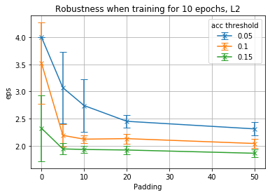
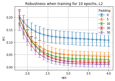
Figure 5: The relationship between attack strength and the padding number $P$ in Table 6 (Top) and the relationship between robust test accuracy and attack strength for different values of $P$ (Bottom). $\ell_{2}$ attack. 10 training epochs.

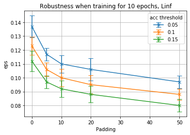
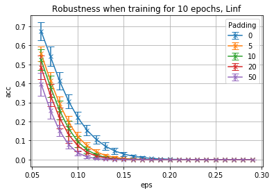
Figure 6: The relationship between attack strength and the padding number $P$ (Top), and the relationship between robust test accuracy and attack strength under different $P$.(Bottom) $\ell_{\infty}$ attack. 10 training epochs.

5.3 Fashion-MNIST

In the same vein as Section 5.2, we verify the effect of increased dimension gap (by padding grey pixel as in the MNIST experiment) on the vulnerability of the model on FMNIST images (Xiao et al., 2017) in Figure 7. Figure 7 illustrates the same pattern of the bottom plot in Figure 6. We use the same convolution network architecture and training setting used for the MNIST experiment (refer to Section D.2.1) averaging over 30 random seeds.

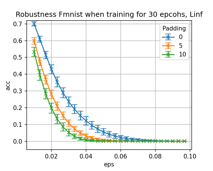
Figure 7: Relationship between robust test accuracy and attack strength under different $P$. $\ell_{\infty}$ attack. 30 training epochs.

5.4 Imagenet Binary Classification

We subset two classes (Dog and Church) from the Imagenet dataset (Deng et al., 2009) and scale all the images to a uniform resolution of 320x320 pixels. In contrast to the FMNIST/MNIST experiments, where we emulate the effect of increasing the dimension gap via adding padding to the images, for Imagenet, we scale the images to different resolutions. The motivation of this experiment is that for higher-resolution images, the ambient dimension increases disproportionately w.r.t the useful features or on-manifold dimensions. From Table 3, even with different resolutions, the intrinsic dimension of the data remains almost constant. Hence, we can use resolution as a surrogate for the intrinsic-ambient dimension gap: higher-resolution images will tend to have a higher dimension gap.

Size($\text{px}^{2}$)	Ambient	LPCA	MLE(k=5)	TwoNN
320	307200	12	22.75	31.27
128	49152	12	21.87	30.08
64	12288	12	20.88	28.93

Table 3: Intrinsic dimension is unchanged even with varying resolution. Imagenet (Dogs+Church).

We rescale the images to 64x64, 128x128, and 320x320 (base) pixels and train Resnet18 models (He et al., 2016) with $10^{-3}$ learning rate and Adam optimizer for 20 epochs in each resolution setting. All models have been trained for 20 epochs for uniform comparison, with $\sim 0.02$ training loss and $~{}99\%$ accuracy averaging over 30 seeds. After the clean training, the models are subjected to $\ell_{\infty}$ PGD attack of varying strengths up to $\epsilon=16/255$.

Figure 8 illustrates that, as the resolution of an image increases, the vulnerability also increases, bolstering our dimension gap argument further.

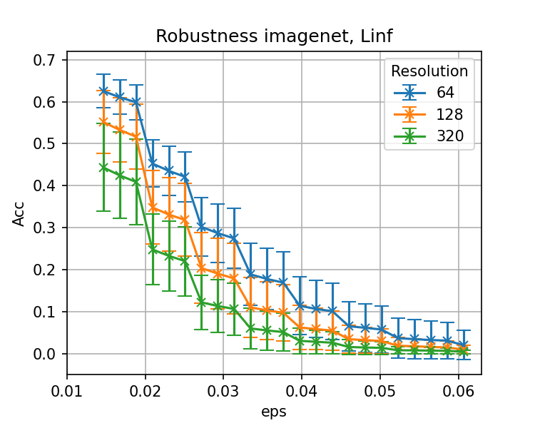
Figure 8: Relationship between robust test accuracy and attack strength under different resolutions. $\ell_{\infty}$ attack.

6 Discussion and Conclusion

We introduce the notion of natural and unnatural attacks residing in on and off manifold space concerning the low dimensional data space. Despite the generalization capabilities of a cleanly trained model on examples drawn from the data space, it will exhibit vulnerabilities to perturbations in both off and on manifold directions. In particular, the off-manifold adversarial perturbations can get arbitrarily small (in $\ell_{\infty}$ norm) with the increase in dimension gap.

Adversarial Training

This work discusses the intrinsic-ambient dimension gap as the root cause for prevalent adversarial attacks in literature. However, we have yet to comment on adversarially trained models that are used to induce robustness to such attacks. We attempt to motivate the success of adversarial training through the lens of our framework. In contrast to clean training, adversarial training aims to minimize the loss over the worst possible attacks the data can exhibit. We can think of adversarial training as clean training on a dataset consisting of adversarial examples of the original data. Even though the original data space is a low dimensional subset of the whole Euclidean space, the dimension of adversarial data space will always be equal to the ambient dimension as we consider a $D$ dimensional $\epsilon$ ball around the original data space. Where $\epsilon$ is a parameter determining the strength of attacks, adversarial data space makes the dimension gap $0$ and, based on our theory, should not induce any off-manifold or unnatural attacks. Thinking of adversarial training as clean training on a much higher dimensional data space also sheds light on the complexity of adversarial training (Schmidt et al., 2018). A higher dimensional data space requires many more observations for a representative sample.

Checklist

1. For all models and algorithms presented, check if you include:

   1. A clear description of the mathematical setting, assumptions, algorithm, and/or model.
      Yes, Refer to Sections 3.1, 3.6, 5 respectively.

   2. An analysis of the properties and complexity (time, space, sample size) of any algorithm.
      Not Applicable

   3. (Optional) Anonymized source code, with specification of all dependencies, including external libraries.
      No, we only have simulations and simple experiments for which the details provided in Section 5, Appendix D suffice.

2. For any theoretical claim, check if you include:

   1. Statements of the full set of assumptions of all theoretical results.
      Yes, Refer section 3.6.

   2. Complete proofs of all theoretical results.
      Yes, Refer to the proofs in Appendix C.

   3. Clear explanations of any assumptions.
      Yes, Refer section 3.6.

3. For all figures and tables that present empirical results, check if you include:

   1. The code, data, and instructions needed to reproduce the main experimental results (either in the supplemental material or as a URL).
      No, We are using simple simulations.

   2. All the training details (e.g., data splits, hyperparameters, how they were chosen).
      Yes, details provided in Section 5, Appendix D.

   3. A clear definition of the specific measure or statistics and error bars (e.g., with respect to the random seed after running experiments multiple times).
      Yes, We provide error bars by running multiple runs.

   4. A description of the computing infrastructure used. (e.g., type of GPUs, internal cluster, or cloud provider). No, Computation is inexpensive and doesn’t need specialized infrastructure.

4. If you are using existing assets (e.g., code, data, models) or curating/releasing new assets, check if you include:

   1. Citations of the creator If your work uses existing assets.
      Yes, Only external asset used is MNIST dataset which has been cited.

   2. The license information of the assets, if applicable.
      Not Applicable

   3. New assets either in the supplemental material or as a URL, if applicable.
      Not Applicable

   4. Information about consent from data providers/curators.
      Not Applicable

   5. Discussion of sensible content if applicable, e.g., personally identifiable information or offensive content. Not Applicable

5. If you used crowdsourcing or conducted research with human subjects, check if you include:

   1. The full text of instructions given to participants and screenshots.
      Not Applicable

   2. Descriptions of potential participant risks, with links to Institutional Review Board (IRB) approvals if applicable.
      Not Applicable

   3. The estimated hourly wage paid to participants and the total amount spent on participant compensation.
      Not Applicable

Appendix A Proof Sketch

We adapt the mathematical techniques used in Frei et al. (2023) to our framework.

• We use the KKT condition in Eq. (4) to connect the neural network weights $\mathbf{w}_{j},b_{j}$ to the data $\tilde{\mathbf{x}}_{i},y_{i}$. Then we can write the outputs at a new sample $\tilde{\mathbf{x}}$ (i.e., ${\cal N}_{{\bm{\theta}}}(\tilde{\mathbf{x}})=\sum_{j=1}^{w}v_{j}\phi(\mathbf{w}_{j}^{\top}\tilde{\mathbf{x}}+b_{j})$) in terms of interactions ($\langle\tilde{\mathbf{x}}_{i},\tilde{\mathbf{x}}\rangle$) between the observed signal $\tilde{\mathbf{x}}_{i}$ and $\tilde{\mathbf{x}}$. For the values of $\langle\tilde{\mathbf{x}}_{i},\tilde{\mathbf{x}}\rangle$, the means $\bm{\mu}^{(r)}$, $r\in[k]$ are nearly orthogonal [3.2 (A2)] and impose $\langle\tilde{\mathbf{x}}_{i},\tilde{\mathbf{x}}\rangle$ to be larger, if $\tilde{\mathbf{x}}_{i},\tilde{\mathbf{x}}$ belong to the same cluster compared to the case when they are from different clusters. This ensures that the neuron output is consistent when a sample is from the same cluster. (Theorem 4.1)

• We further study the adversarial attack. As discussed in Section 3.5, $\mathbf{w}_{j}$ can be decomposed into $\mathbf{P}_{o}\mathbf{w}_{j}$ and $\mathbf{P}\mathbf{w}_{j}$. We design perturbations $\mathbf{z}_{\shortparallel}$ and $\mathbf{z}_{\perp}$, such that $\mathbf{P}_{o}\mathbf{w}_{j}^{\top}\mathbf{z}_{\shortparallel}$ and $\mathbf{P}\mathbf{w}_{j}^{\top}\mathbf{z}_{\perp}$ can be made arbitrarily large in magnitude compared to $\mathbf{w}_{j}^{\top}\tilde{\mathbf{x}}$. For $\mathbf{z}=\mathbf{z}_{\perp},\mathbf{z}_{\shortparallel}$, we have $\mathbf{w}_{j}^{\top}(\tilde{\mathbf{x}}+\mathbf{z})=\mathbf{w}_{j}^{\top}\tilde{\mathbf{x}}+\mathbf{P}\mathbf{w}_{j}^{\top}\mathbf{z}_{\perp},\mathbf{w}_{j}^{\top}\tilde{\mathbf{x}}+\mathbf{P}_{o}\mathbf{w}_{j}^{\top}\mathbf{z}_{\shortparallel}$; thus we can manipulate the sign of each neuron after perturbation. (Theorem 4.2)

Appendix B Definitions and short hands

$\bar{\zeta}$ is a shorthand notation to bound $\bm{\zeta}^{(r)}+\bm{\omega}_{i}$ from above, for any $i\in[n],r\in[k]$ with very high probability. $\bar{\omega}$ will denote the upper bound for $\bm{\omega}_{i}$ for $i\in[n]$. If assumption 3.2 hold then $\bar{\omega}\leq 1$ and $\bar{\zeta}$ can be set to a constant in Definition B.2.

Definition B.1 (Semi-inner product).

For any positive semi-definite matrix $A$ we can define a semi-inner product $\langle,\rangle_{A}$ such that for all $a,b\in\mathbb{R}^{D}$:

$$\langle a,b\rangle_{A}=a^{T}Ab$$

If $A$ is a projection matrix, then $\langle a,b\rangle_{A}=\langle Aa,Ab\rangle$ where $\langle,\rangle$ is the standard inner product.

Definition B.2 (Constants).

$$c_{2} =1+\sqrt{2};\bar{\zeta}^{2}=1+2\tau\sqrt{\frac{13D}{8}}+\frac{13D\tau^{2}}{8}$$

$$\Delta =2c_{2}\sqrt{d}\ln(d)$$

$$\epsilon_{x} =\bar{\zeta}^{2}+2\bar{\zeta}\sqrt{d}c_{2}$$

$$\epsilon_{\xi} =\bar{\zeta}^{2}+2\bar{\zeta}\sqrt{2}\ln{d}$$

$$\epsilon_{x\xi} =\bar{\zeta}^{2}+\bar{\zeta}(2\sqrt{2}\ln{d}+\sqrt{d}c_{2})$$

$$\epsilon_{\zeta}^{\shortparallel} =\left(\sqrt{2}\ln d+\bar{\omega}\right)\left\|\mathbf{P}_{o}\bm{\zeta}\right\|;\,\epsilon_{\zeta}^{\perp}=\bar{\omega}\left\|\mathbf{P}\bm{\zeta}\right\|$$

$$p =\max_{i\neq j}|\langle\bm{\mu}^{(i)},\bm{\mu}^{(j)}\rangle|$$

$$\Delta^{\prime} =\Delta+\epsilon_{x}$$

Appendix C Proofs

Lemma C.0.1 (Properties).

Given $\mathbf{x}$ belongs to the $r^{th}$ cluster, if the assumptions 3.2 hold and $\left\|\bm{\zeta}^{(r)}+\bm{\omega}\right\|\leq\bar{\zeta}$ for any $r\in[k]$, we have the following properties:

1. $|\langle\bm{\xi}_{i},\bm{\xi}\rangle|<\Delta$ and $|\langle\tilde{\bm{\xi}}_{i},\tilde{\bm{\xi}}\rangle|\leq\Delta+\epsilon_{\xi}\leq\Delta^{\prime}$.

2. $|\langle\mathbf{x}_{i},\bm{\xi}\rangle|\leq\Delta$ and $|\langle\tilde{\mathbf{x}}_{i},\tilde{\bm{\xi}}\rangle|\leq\Delta+\epsilon_{x\xi}\leq\Delta^{\prime}$

3. If $i\not\in I^{(r)}$ then $|\langle\mathbf{x}_{i},\mathbf{x}\rangle|\leq p+\Delta$ and $|\langle\tilde{\mathbf{x}}_{i},\tilde{\mathbf{x}}\rangle|\leq p+\Delta^{\prime}$

4. If $i\in I^{(r)}$ then $|\langle\mathbf{x}_{i},\mathbf{x}\rangle-d|\leq\Delta$ and $|\langle\tilde{\mathbf{x}}_{i},\tilde{\mathbf{x}}\rangle-d|\leq\Delta^{\prime}$

Proof.

Using cauchy-schwartz, (A3) and $\ln x<\sqrt{x}$; we have:

1. $|\langle\bm{\xi}_{i},\bm{\xi}\rangle|\leq|2\ln^{2}d|<2\sqrt{d}\ln d<\Delta$. Consequently,

   $$|\langle\tilde{\bm{\xi}}_{i},\tilde{\bm{\xi}}\rangle| =|\langle\mathbf{M}\bm{\xi}_{i}+\bm{\zeta}^{(r^{\prime})}+\bm{\omega}_{i},\mathbf{M}\bm{\xi}+\bm{\zeta}^{(r)}+\bm{\omega}\rangle|$$

   $$=|\langle\bm{\xi}_{i},\bm{\xi}\rangle+\langle\bm{\zeta}^{(r^{\prime})}+\bm{\omega}_{i},\bm{\zeta}^{(r)}+\bm{\omega}\rangle+\langle\mathbf{M}\bm{\xi}_{i},\bm{\zeta}^{(r)}+\bm{\omega}\rangle+\langle\mathbf{M}\bm{\xi},\bm{\zeta}^{(r^{\prime})}+\bm{\omega}_{i}\rangle|$$

   $$\leq|\langle\bm{\xi}_{i},\bm{\xi}\rangle|+\bar{\zeta}^{2}+2\|\mathbf{M}\|_{op}\sqrt{2}\ln d\cdot\bar{\zeta}\leq\Delta+\epsilon_{\xi}\leq\Delta+\epsilon_{x}=\Delta^{\prime}$$

   $\|\mathbf{M}\|_{op}=1$ as $\mathbf{M}$ has orthogonal columns.

2. $|\langle\mathbf{x}_{i},\bm{\xi}\rangle|=|\langle\bm{\mu}^{(r^{\prime})}+\bm{\xi}_{i},\bm{\xi}\rangle|\leq|\langle\bm{\mu}^{(r^{\prime})},\bm{\xi}\rangle|+|\langle\bm{\xi}_{i},\bm{\xi}\rangle|\leq\sqrt{2}\sqrt{d}\ln d+2\ln^{2}d<2c_{2}\sqrt{d}\ln d=\Delta$.

   $$\langle\tilde{\mathbf{x}}_{i},\tilde{\bm{\xi}}\rangle| =|\langle\mathbf{M}\mathbf{x}_{i}+\bm{\zeta}^{(r^{\prime})}+\bm{\omega}_{i},\mathbf{M}\bm{\xi}+\bm{\zeta}^{(r)}+\bm{\omega}\rangle|$$

   $$\leq|\langle\mathbf{x}_{i},\bm{\xi}\rangle+\langle\bm{\zeta}^{(r^{\prime})}+\bm{\omega}_{i},\bm{\zeta}^{(r)}+\bm{\omega}\rangle+\langle\mathbf{M}\bm{\xi}_{i},\bm{\zeta}^{(r)}+\bm{\omega}\rangle+\langle\mathbf{M}\underbrace{\mathbf{x}_{i}}_{\bm{\mu}^{(r^{\prime})}+\bm{\xi}_{i}},\bm{\zeta}^{(r^{\prime})}+\bm{\omega}_{i}\rangle|$$

   $$\leq\Delta+\bar{\zeta}^{2}+\|\mathbf{M}\|_{op}\sqrt{2}\ln d\cdot\bar{\zeta}+\|\mathbf{M}\|_{op}(\sqrt{d}+\sqrt{2}\ln d)\cdot\bar{\zeta}$$

   $$\leq\Delta+\epsilon_{x\xi}\leq\Delta+\epsilon_{x}=\Delta^{\prime}$$

3. If $i\not\in I^{(r)}$ then, $|\langle\mathbf{x}_{i},\mathbf{x}\rangle|=|\langle\bm{\mu}^{(r^{\prime})}+\bm{\xi}_{i},\bm{\mu}^{(r)}+\bm{\xi}\rangle|\leq|\langle\bm{\mu}^{(r^{\prime})},\bm{\mu}^{(r)}\rangle|+|\langle\bm{\xi}_{i},\bm{\xi}\rangle|\leq p+\Delta$.
   Similarly, $|\langle\tilde{\mathbf{x}}_{i},\tilde{\mathbf{x}}\rangle|=|\langle\tilde{\bm{\mu}}^{(r^{\prime})}+\tilde{\bm{\xi}}_{i},\tilde{\bm{\mu}}^{(r)}+\tilde{\bm{\xi}}\rangle|\leq|\langle\tilde{\bm{\mu}}^{(r^{\prime})},\tilde{\bm{\mu}}^{(r)}\rangle|+|\langle\tilde{\bm{\xi}}_{i},\tilde{\bm{\xi}}\rangle|=|\langle\bm{\mu}^{(r^{\prime})},\bm{\mu}^{(r)}\rangle|+|\langle\tilde{\bm{\xi}}_{i},\tilde{\bm{\xi}}\rangle|\leq p+\Delta^{\prime}$.

4. If $i\in I^{(r)}$ then, $|\langle\mathbf{x}_{i},\mathbf{x}\rangle-d|=|\langle\bm{\mu}^{(r)}+\bm{\xi}_{i},\bm{\mu}^{(r)}+\bm{\xi}\rangle-d|\leq\|\bm{\mu}^{(r)}\|-d+\langle\bm{\xi}_{i},\bm{\xi}\rangle|\leq 0+\Delta$.
   Similarly, $|\langle\tilde{\mathbf{x}}_{i},\tilde{\mathbf{x}}\rangle-d|=|\langle\tilde{\bm{\mu}}^{(r)}+\tilde{\bm{\xi}}_{i},\tilde{\bm{\mu}}^{(r)}+\tilde{\bm{\xi}}\rangle-d|\leq\|\bm{\mu}^{(r)}\|-d+\langle\tilde{\bm{\xi}}_{i},\tilde{\bm{\xi}}\rangle|\leq 0+\Delta^{\prime}$.

∎

C.1 High probability statements

In this section, we show that any of the following events hold with a very high probability for any $q\in[k]$ :

1. $\left\|\bm{\zeta}^{(q)}\right\|\asymp\tau\sqrt{D}$, in particular $\tau\sqrt{\frac{D}{2}}<\left\|\bm{\zeta}^{(q)}\right\|<\tau\sqrt{\frac{13D}{8}}$

2. $\bm{\zeta}^{(q)\top}\mathbf{P}\bm{\zeta}^{(q)}\asymp g\tau^{2}$, in particular $\frac{g\tau^{2}}{2}<\bm{\zeta}^{(q)\top}\mathbf{P}\bm{\zeta}^{(q)}<\frac{13g\tau^{2}}{8}$

3. $\bm{\zeta}^{(q)\top}\mathbf{P}_{o}\bm{\zeta}^{(q)}\asymp d\tau^{2}$, in particular $\frac{d\tau^{2}}{2}<\bm{\zeta}^{(q)\top}\mathbf{P}_{o}\bm{\zeta}^{(q)}<\frac{13d\tau^{2}}{8}$

4. $\left\|\mathbf{P}\bm{\zeta}^{(q)}\right\|_{\infty}={\cal O}{\left(\tau\sqrt{2\log(2g)}\right)}$, in particular $\left\|\mathbf{P}\bm{\zeta}^{(q)}\right\|_{\infty}<3\tau\sqrt{2\log(2g)}$

5. $\left\|\mathbf{P}_{o}\bm{\zeta}^{(q)}\right\|_{\infty}={\cal O}{\left(\tau\sqrt{2\log(2d)}\right)}$, in particular $\left\|\mathbf{P}_{o}\bm{\zeta}^{(q)}\right\|_{\infty}<3\tau\sqrt{2\log(2d)}$

6. $k\cdot\left(\max_{i\neq j}|\langle\bm{\zeta}^{(i)},\bm{\zeta}^{(j)}\rangle_{\mathbf{P}}|+\epsilon^{\perp}_{\zeta}\right)<\frac{1}{10}\cdot\left(\bm{\zeta}^{(q)T}\mathbf{P}\bm{\zeta}^{(q)}-\epsilon^{\perp}_{\zeta}\right)$

7. $k\cdot\left(\max_{i\neq j}|\langle\bm{\zeta}^{(i)},\bm{\zeta}^{(j)}\rangle_{\mathbf{P}_{o}}|+\epsilon^{\shortparallel}_{\zeta}\right)<\frac{1}{10}\cdot\left(\bm{\zeta}^{(q)T}\mathbf{P}_{o}\bm{\zeta}^{(q)}-\epsilon^{\shortparallel}_{\zeta}\right)$

Lemma C.1.1.

$\left\|\bm{\zeta}^{(q)}\right\|\asymp\tau\sqrt{D}=\sqrt{h}$ , $\bm{\zeta}^{(q)\top}\mathbf{P}\bm{\zeta}^{(q)}\asymp g\tau^{2}$ and $\bm{\zeta}^{(q)\top}\mathbf{P}_{o}\bm{\zeta}^{(q)}\asymp d\tau^{2}$ w.h.p. for any $q\in[k]$.
Specifically,

$$P(\frac{\bm{\zeta}^{(q)\top}\mathbf{P}\bm{\zeta}^{(q)}}{\tau^{2}}>\frac{13g}{8})\leq e^{-\frac{g}{16}};\,P(\frac{\bm{\zeta}^{(q)\top}\mathbf{P}\bm{\zeta}^{(q)}}{\tau^{2}}<\frac{g}{2})\leq e^{-\frac{g}{16}}$$

$$P(\frac{\bm{\zeta}^{(q)\top}\mathbf{P}_{o}\bm{\zeta}^{(q)}}{\tau^{2}}>\frac{13d}{8})\leq e^{-\frac{d}{16}};\,P(\frac{\bm{\zeta}^{(q)\top}\mathbf{P}_{o}\bm{\zeta}^{(q)}}{\tau^{2}}<\frac{d}{2})\leq e^{-\frac{d}{16}}$$

$$P(\left\|\bm{\zeta}^{(q)}\right\|>\tau\sqrt{\frac{13D}{8}})\leq e^{-\frac{D}{16}};\,P(\left\|\bm{\zeta}^{(q)}\right\|<\tau\sqrt{\frac{D}{2}})\leq e^{-\frac{D}{16}}$$

Proof.

As $\mathbf{P},\mathbf{P}_{o}$ are projection matrices of rank $g,d$ respectively, they are idempotent and hence $\bm{\zeta}^{(q)\top}\mathbf{P}\bm{\zeta}^{(q)}\tau^{-2}\sim\chi^{2}(g)\,,\bm{\zeta}^{(q)\top}\mathbf{P}_{o}\bm{\zeta}^{(q)}\tau^{-2}\sim\chi^{2}(d)$. Also, $\left\|\bm{\zeta}\right\|^{2}\tau^{-2}\sim\chi^{2}(D)$.
Using Laurent and Massart (2000) lemma 1:

$$P(\frac{\bm{\zeta}^{(q)\top}\mathbf{P}\bm{\zeta}^{(q)}}{\tau^{2}}>g+2\sqrt{g}\sqrt{x}+2x)\leq e^{-x};\,P(\frac{\bm{\zeta}^{(q)\top}\mathbf{P}\bm{\zeta}^{(q)}}{\tau^{2}}<g-2\sqrt{g}\sqrt{x})\leq e^{-x}$$

Setting $x=\frac{g}{16}$ we get:

$$P(\frac{\bm{\zeta}^{(q)\top}\mathbf{P}\bm{\zeta}^{(q)}}{\tau^{2}}>\frac{13g}{8})\leq e^{-\frac{g}{16}};\,P(\frac{\bm{\zeta}^{(q)\top}\mathbf{P}\bm{\zeta}^{(q)}}{\tau^{2}}<\frac{g}{2})\leq e^{-\frac{g}{16}}$$

Using union bound we have $P(\frac{g}{2}<\frac{\bm{\zeta}^{(q)\top}\mathbf{P}\bm{\zeta}^{(q)}}{\tau^{2}}<\frac{13g}{8})\geq 1-2e^{-\frac{g}{16}}$. One can get an identical statement for $\bm{\zeta}^{(q)\top}\mathbf{P}_{o}\bm{\zeta}^{(q)}$ replacing $g$ with $d$.
Similarly, one can get

$$P(\frac{\left\|\bm{\zeta}^{(q)}\right\|^{2}}{\tau^{2}}>\frac{13D}{8})\leq e^{-\frac{D}{16}};\,P(\frac{\left\|\bm{\zeta}^{(q)}\right\|^{2}}{\tau^{2}}<\frac{D}{2})\leq e^{-\frac{D}{16}}$$

Consequently, $P(\frac{D}{2}<\frac{\left\|\bm{\zeta}^{(q)}\right\|^{2}}{\tau^{2}}<\frac{13D}{8})\geq 1-2e^{-\frac{D}{16}}$ ∎

Lemma C.1.2.

For the projection matrix $\mathbf{P}$ for every $i\in[D]$ we have $0<p_{ii}<1$. Where $p_{ij}$ is the entry in $i^{th}$ row and $j^{th}$ column of $\mathbf{P}$. Also, there exists an indexing set $L$ of length $d$ such that for all $i\in L$, $p_{ii}=0$.

Proof.

As $\mathbf{P}^{\top}=\mathbf{P}$ and $\mathbf{P}^{2}=\mathbf{P}$, we have $p_{ii}=p_{ii}^{2}+\sum_{i\neq j}p_{ij}^{2}$.
This means $p_{ii}^{2}\leq p_{ii}$, hence $0<p_{ii}<1$.
Considering, the eigenvalue decomposition of $\mathbf{P}=O^{T}\Lambda O$ WLOG we can assume that $\Lambda$ is ordered such that the first $g$ diagonal elements are $1$ and the rest $d$ diagonal elements are $0$. One can check that this enforces the first $g$ diagonal elements of $\mathbf{P}$ to non-zero and the rest $d$ diagonal elements to be $0$.
In general $\Lambda$ won’t be ordered hence an indexing set $L$ can be used corresponding to the $0$ eigenvalues; and $p_{ii}=0$ for $i\in L$. ∎

Corollary C.1.1.

For the projection matrix $\mathbf{P}_{o}$ for every $i\in[D]$ we have $0<r_{ii}<1$. Where $r_{ij}$ is the entry in $i^{th}$ row and $j^{th}$ column of $\mathbf{P}_{o}$. Also, there exists an indexing set $L_{o}$ of length $g$ such that for all $i\in L_{o}$, $r_{ii}=0$.

Proof.

Notice that, $\mathbf{P}_{o}=\mathbf{I}-\mathbf{P}=O^{\top}(\mathbf{I}-\Lambda)O$. Mimicking the arguments of Lemma C.1.2 the proof follows. ∎

Lemma C.1.3.

$\left\|\mathbf{P}\bm{\zeta}^{(q)}\right\|_{\infty}={\cal O}{\left(\tau\sqrt{2\log(2g)}\right)}\,,\left\|\mathbf{P}_{o}\bm{\zeta}^{(q)}\right\|_{\infty}={\cal O}{\left(\tau\sqrt{2\log(2d)}\right)}$ w.h.p. for any $q\in[k]$.
Specifically,

$$P\left[\|\mathbf{P}\bm{\zeta}^{(q)}\|_{\infty}>3\tau\sqrt{2\log(2g)}\right]\leq e^{-4\log(2g)}$$

$$P\left[\|\mathbf{P}_{o}\bm{\zeta}^{(q)}\|_{\infty}>3\tau\sqrt{2\log(2d)}\right]\leq e^{-4\log(2d)}$$

Proof.

First we will bound $\operatorname*{\mathbb{E}}(\|\mathbf{P}\bm{\zeta}\|_{\infty})$ for any $\bm{\zeta}\sim N(0,\tau^{2}\mathbf{I}_{D})$.
Let, $Z=\|\mathbf{P}\bm{\zeta}\|_{\infty}$ equivalently $Z=\max\limits_{i\in[D]}\max\{(\mathbf{P}\bm{\zeta})_{i},-(\mathbf{P}\bm{\zeta})_{i}\}$.
We can define $X_{i}=(\mathbf{P}\bm{\zeta})_{i}\sim N(0,\tau^{2}p_{ii})$ and $X_{2i}=(-\mathbf{P}\bm{\zeta})_{i}\sim N(0,\tau^{2}p_{ii})$. Where $p_{ii}$ is the $i^{th}$ diagonal element of $\mathbf{P}$. From Lemma C.1.2 there exists an indexing set $L$ such that $p_{ii}=0\,\forall i\in L$. This implies $X_{i}=0,X_{2i}=0\,\forall i\in L$. Hence, $Z=\max\limits_{i\in[D]\setminus L}\max\{(\mathbf{P}\bm{\zeta})_{i},-(\mathbf{P}\bm{\zeta})_{i}\}$.
By Jensen’s inequality for any $t>0$, we have

$$\exp\{t\mathbb{E}[Z]\}\leq\mathbb{E}\exp\{tZ\}=\mathbb{E}\max\limits_{i\in[2D]\setminus(L\cup 2L)}\exp\{tX_{i}\} \leq\sum_{i\in[2D]\setminus(L\cup 2L)}\mathbb{E}[\exp\{tX_{i}\}]$$

$$\overset{(i)}{=}\sum_{i\in[D]\setminus L}2\exp\{t^{2}p_{ii}\tau^{2}/2\}\overset{(ii)}{\leq}2g\exp\{t^{2}\tau^{2}/2\}$$

$(i)$ uses the moment-generating function for Gaussian. $(ii)$ uses the fact that $p_{ii}<1$ and $|[D]\setminus L|=g$ from Lemma C.1.2.

$$\operatorname*{\mathbb{E}}[Z]\leq\frac{\log 2g}{t}+\frac{t\tau^{2}}{2}$$

Setting $t=\frac{\sqrt{2\log 2g}}{\tau}$ we get $\operatorname*{\mathbb{E}}[Z]\leq\tau\sqrt{2\log(2g)}$. For any $u>0$ we have

$$P[Z>\tau\sqrt{2\log(2g)}+u] \leq P(Z>\operatorname*{\mathbb{E}}Z+u)$$

$$\overset{(iii)}{\leq}e^{-\frac{u^{2}}{2\tau^{2}\max_{i}p_{ii}}}\leq e^{-\frac{u^{2}}{2\tau^{2}}}$$

Where, $(iii)$ uses Borell-TIS inequality Adler and Taylor (2007).
Setting, $u=2\tau\sqrt{2\log(2g)}$ we get $P(Z>3\tau\sqrt{2\log(2g)})\leq e^{-4\log(2g)}$. Finally $P(\|\mathbf{P}\bm{\zeta}\|_{\infty}<3\tau\sqrt{2\log(2g)})=1-e^{-4\log(2g)}$. One can get an identical result for $\mathbf{P}_{o}\bm{\zeta}^{(q)}$ replacing $g\to d$ and using Corollary C.1.1 instead of C.1.2. ∎

Lemma C.1.4.

For any $\delta>0$ and $i\neq j\in[k]$; $|\langle\bm{\zeta}^{(i)},\bm{\zeta}^{(j)}\rangle_{\mathbf{P}}|,|\langle\bm{\zeta}^{(i)},\bm{\zeta}^{(j)}\rangle_{\mathbf{P}_{o}}|\leq\delta$ w.h.p.
Specifically,

$$P\left[\langle\bm{\zeta}^{(i)},\bm{\zeta}^{(j)}\rangle_{\mathbf{P}}\geq\delta\right]\leq 4e^{-\frac{2\delta}{\sqrt{8g}\tau^{2}}} ;P\left[\langle\bm{\zeta}^{(i)},\bm{\zeta}^{(j)}\rangle_{\mathbf{P}}\leq-\delta\right]\leq 4e^{-\frac{2\delta}{\sqrt{8g}\tau^{2}}}$$

$$P\left[\langle\bm{\zeta}^{(i)},\bm{\zeta}^{(j)}\rangle_{\mathbf{P}_{o}}\geq\delta\right]\leq 4e^{-\frac{2\delta}{\sqrt{8d}\tau^{2}}} ;P\left[\langle\bm{\zeta}^{(i)},\bm{\zeta}^{(j)}\rangle_{\mathbf{P}_{o}}\leq-\delta\right]\leq 4e^{-\frac{2\delta}{\sqrt{8d}\tau^{2}}}$$

Proof.

Let, $Z_{1}=\mathbf{P}\bm{\zeta}^{(i)}\sim N(0,\tau^{2}\mathbf{P})$ and $Z_{2}=\bm{\zeta}^{(j)}\sim N(0,\tau^{2}\mathbf{I}_{D})$ for $i\neq j$.

$$\langle\bm{\zeta}^{(i)},\bm{\zeta}^{(j)}\rangle_{\mathbf{P}}=\bm{\zeta}^{(i)\top}\mathbf{P}\bm{\zeta}^{(j)}=(\mathbf{P}\bm{\zeta}^{(i)})^{\top}\bm{\zeta}^{(j)}=Z_{1}^{T}Z_{2}$$

The inner product can be expressed as: $Z_{1}^{T}Z_{2}=\|Z_{1}\|\cdot\frac{Z_{1}}{\|Z_{1}\|}^{\top}Z_{2}$.
Notice that, $\frac{Z_{1}}{\|Z_{1}\|}^{\top}Z_{2}\sim N(0,\tau^{2})$ and is independent of $Z_{1}$. Hence, using the standard Gaussian- tail bounds for $\delta>0,C\geq 1$.

$$P\left(\frac{Z_{1}}{\|Z_{1}\|}^{\top}Z_{2}>\frac{\delta}{C}\right)\leq e^{-\frac{\delta^{2}}{2C^{2}\tau^{2}}}$$ (6)

We can also get a concentration inequality for $\|Z_{1}\|$, using Ledoux (2006) formula (3.5).

$$P\left(\|Z_{1}\|>C\right) \leq 4e^{-\frac{C^{2}}{8\operatorname*{\mathbb{E}}(\|Z_{1}\|^{2})}}$$

$$\overset{(i)}{=}4e^{-\frac{C^{2}}{8g\tau^{2}}}$$ (7)

Where $(i)$ follows from the fact that $\|Z_{1}\|^{2}\tau^{-2}\sim\chi^{2}(g)$, hence $\operatorname*{\mathbb{E}}(\|Z_{1}\|^{2})=g\tau^{2}$.
Combining, Eq. (7) and Eq. (6), we have:

$$P(Z_{1}^{T}Z_{2}>\delta)\leq 4\exp\left(-\frac{\delta^{2}}{2C^{2}\tau^{2}}-\frac{C^{2}}{8g\tau^{2}}\right)$$

Setting $C^{2}=\sqrt{4g}\delta$ we get :

$$P(Z_{1}^{T}Z_{2}>\delta)\leq 4\exp\left(-\frac{\delta}{\sqrt{4g}\tau^{2}}\right)$$

One can convince themselves, that $Z_{1}^{T}Z_{2}$ has a symmetric distribution it is a product of Gaussians. Hence, we also have:

$$P(Z_{1}^{T}Z_{2}<-\delta)\leq 4\exp\left(-\frac{\delta}{\sqrt{4g}\tau^{2}}\right)$$

Using the union bound,

$$P(|Z_{1}^{T}Z_{2}|<\delta)\geq 1-8\exp\left(-\frac{\delta}{\sqrt{4g}\tau^{2}}\right)$$

The proof for $\langle\bm{\zeta}^{(i)},\bm{\zeta}^{(j)}\rangle_{\mathbf{P}_{o}}$ is identical. ∎

Lemma C.1.5.

For all $r\in[k]$ and $j\neq r$ consider the following events hold with high probability:

1. $\frac{g\tau^{2}}{2}<\bm{\zeta}^{(r)\top}\mathbf{P}\bm{\zeta}^{(r)}=\|\mathbf{P}\bm{\zeta}^{(r)}\|^{2}<\frac{13g\tau^{2}}{8}$

2. $\frac{D\tau^{2}}{2}<\|\bm{\zeta}^{(r)}\|^{2}<\frac{13D\tau^{2}}{8}$

3. $\left\|\mathbf{P}\bm{\zeta}^{(r)}\right\|_{\infty}<3\tau\sqrt{2\log(2g)}$

4. $\max_{r\neq j}|\langle\bm{\zeta}^{(r)},\bm{\zeta}^{(j)}\rangle_{\mathbf{P}}|\leq\frac{g\tau^{2}}{20k}-\frac{10k+1}{10k}\sqrt{\frac{13g\tau^{2}}{8}}=c_{3}(g,\tau,k)\asymp\left(\frac{g\tau^{2}}{k}\right)$

Specifically,

$$P\left(k\left(\max_{i\neq j}|\langle\bm{\zeta}^{(i)},\bm{\zeta}^{(j)}\rangle_{\mathbf{P}}|+\epsilon^{\perp}_{\zeta}\right)<\frac{1}{10}\cdot[\bm{\zeta}^{(r)\top}\mathbf{P}\bm{\zeta}^{(r)}-\epsilon^{\perp}_{\zeta}]\right)\geq 1-\delta_{1}$$

$$\delta_{1}=\left(4k(k-1)\exp{\left(-\frac{c_{3}}{\sqrt{4g}\tau^{2}}\right)}+2k\exp(-\frac{g}{16})+2k\exp(-\frac{D}{16})+k\exp(-4\log 2g)\right)$$

With all events (1-4) being satisfied.

Proof.

If the above events hold true then $\epsilon^{\perp}_{\zeta}=\bar{\omega}\left\|\mathbf{P}\bm{\zeta}\right\|\leq\sqrt{\frac{13g\tau^{2}}{8}}$.
Using Lemma C.1.5 with $\delta=c_{3}(g,\tau,k)$ and due to the assumption of $c_{3}(g,\tau,k)>0$ we have:

$$P\left[\langle\bm{\zeta}^{(r)},\bm{\zeta}^{(j)}\rangle_{\mathbf{P}}\geq c_{3}(g,\tau,k)\right]\leq 4\exp{-\frac{c_{3}}{\sqrt{4g}\tau^{2}}}$$ (8)

$$P\left[\langle\bm{\zeta}^{(r)},\bm{\zeta}^{(j)}\rangle_{\mathbf{P}}\leq-c_{3}(g,\tau,k)\right]\leq 4\exp{-\frac{c_{3}}{\sqrt{4g}\tau^{2}}}$$

Let,

$$P(A) =P\{\bigcup_{r\neq j}\left[\langle\bm{\zeta}^{(r)},\bm{\zeta}^{(j)}\rangle_{\mathbf{P}}\geq c_{3}\cup\langle\bm{\zeta}^{(r)},\bm{\zeta}^{(j)}\rangle_{\mathbf{P}}\leq-c_{3}\right]\}\overset{(i)}{\leq}4k(k-1)\exp{-\frac{c_{3}}{\sqrt{4g}\tau^{2}}}$$

$$P(B) =P\{\bigcup_{r\in[k]}\left[\bm{\zeta}^{(r)\top}\mathbf{P}\bm{\zeta}^{(r)}\geq\frac{13g\tau^{2}}{8}\cup\bm{\zeta}^{(r)\top}\mathbf{P}\bm{\zeta}^{(r)}\leq\frac{g\tau^{2}}{2}\right]\}\overset{(ii)}{\leq}2k\exp(-\frac{g}{16})$$

$$P(C) =P\{\bigcup_{r\in[k]}\left[\|\bm{\zeta}^{(r)}\|^{2}\geq\frac{13D\tau^{2}}{8}\cup\|\bm{\zeta}^{(r)}\|^{2}\leq\frac{D\tau^{2}}{2}\right]\}\overset{(iii)}{\leq}2k\exp(-\frac{D}{16})$$

$$P(D) =P\{\bigcup_{r\in[k]}\left\|\mathbf{P}\bm{\zeta}^{(r)}\right\|_{\infty}>3\tau\sqrt{2\log(2g)}\}\overset{(iv)}{\leq}k\exp(-4\log 2g)$$

Where $(i)$ uses Eq. (8); $(ii),(iii)$ uses Lemma C.1.1 and $(iv)$ uses Lemma C.1.3, along with the Union bound. The probability that all of the high-probability events happen can be computed by the union bound: $1-P(A\cup B\cup C\cup D)\geq 1-\left(4k(k-1)\exp{(-\frac{c_{3}}{\sqrt{4g}\tau^{2}})}+2k\exp(-\frac{g}{16})+2k\exp(-\frac{D}{16})+k\exp(-4\log 2g)\right)$.
Hence,

$$P\left(k\left(\max_{i\neq j}|\langle\bm{\zeta}^{(i)},\bm{\zeta}^{(j)}\rangle_{\mathbf{P}}|+\epsilon^{\perp}_{\zeta}\right)<\frac{1}{10}\cdot[\bm{\zeta}^{(r)\top}\mathbf{P}\bm{\zeta}^{(r)}-\epsilon^{\perp}_{\zeta}]\right)\geq P\left(k\left(\max_{i\neq j}|\langle\bm{\zeta}^{(i)},\bm{\zeta}^{(j)}\rangle_{\mathbf{P}}|\right)<c_{3}(g,\tau,k)\right)$$

$$\geq 1-\left(4k(k-1)\exp{(-\frac{c_{3}}{\sqrt{4g}\tau^{2}})}+2k\exp(-\frac{g}{16})+2k\exp(-\frac{D}{16})+k\exp(-4\log 2g)\right)$$

∎

Lemma C.1.6.

For some $q\in[k]$, let $V_{q}=\sum_{r\in[k]}y^{(r)}y^{(q)}\langle\tilde{\bm{\mu}}^{(q)},\bm{\zeta}^{(r)}\rangle_{\mathbf{P}_{o}}$. Then w.h.p. $|V_{q}|<\frac{1}{10}\cdot c_{4}(d,\tau,k,p)$, where $c_{4}(d,\tau,k,p)=d-\Delta^{\prime}-k(p+\Delta^{\prime})+\frac{9}{10}\cdot\left(\frac{d\tau^{2}}{2}-\sqrt{\frac{13d\tau^{2}}{8}}(\sigma\sqrt{2}\ln d+1)\right)$

Proof.

As each $\bm{\zeta}^{(r)}\overset{i.i.d.}{\sim}N(0,\tau^{2}\mathbf{I}_{D})$ and $\|\tilde{\bm{\mu}}\|^{2}=d$, we have $y^{(r)}y^{(q)}\langle\tilde{\bm{\mu}}^{(q)},\bm{\zeta}^{(r)}\rangle_{\mathbf{P}_{o}}\overset{i.i.d}{\sim}N(0,\tau^{2}d)$. Consequently, $V_{q}\sim N(0,\tau^{2}dk)$.
Using gaussian tail bound we have:

$$P\left(|V_{q}|\geq\frac{1}{10}\cdot c_{4}(d,\tau,k,p)\right)\leq 2\exp\left(-\frac{c_{4}^{2}}{20\tau^{2}dk}\right)$$

∎

Lemma C.1.7.

For all $r\in[k]$ and $j\neq r$ consider the following events hold with high probability:

1. $\frac{d\tau^{2}}{2}<\bm{\zeta}^{(r)\top}\mathbf{P}_{o}\bm{\zeta}^{(r)}=\|\mathbf{P}_{o}\bm{\zeta}^{(r)}\|^{2}<\frac{13d\tau^{2}}{8}$

2. $\frac{D\tau^{2}}{2}<\|\bm{\zeta}^{(r)}\|^{2}<\frac{13D\tau^{2}}{8}$

3. $\left\|\mathbf{P}_{o}\bm{\zeta}^{(r)}\right\|_{\infty}<3\tau\sqrt{2\log(2d)}$

4. $|V_{r}|<\frac{1}{10}\cdot c_{4}(d,\tau,k,p)$

5. $\max_{r\neq j}|\langle\bm{\zeta}^{(r)},\bm{\zeta}^{(j)}\rangle_{\mathbf{P}_{o}}|\leq\frac{d\tau^{2}}{20k}-\frac{10k+1}{10k}\sqrt{\frac{13d\tau^{2}}{8}}(\sigma\sqrt{2\ln d+1})=c_{5}(d,\tau,k)\asymp\left(\frac{d\tau^{2}}{k}\right)$

Specifically,

$$P\left(k\left(\max_{i\neq j}|\langle\bm{\zeta}^{(i)},\bm{\zeta}^{(j)}\rangle_{\mathbf{P}_{o}}|+\epsilon^{\shortparallel}_{\zeta}\right)<\frac{1}{10}\cdot[\bm{\zeta}^{(r)\top}\mathbf{P}_{o}\bm{\zeta}^{(r)}-\epsilon^{\shortparallel}_{\zeta}]\right)\geq 1-\delta_{2}$$

$$\delta_{2}=\left(4k(k-1)\exp{\left(-\frac{c_{5}}{\sqrt{4d}\tau^{2}}\right)}+2k\exp(-\frac{d}{16})+2k\exp(-\frac{D}{16})+k\exp(-4\log 2d)+2k\exp(-\frac{c_{4}^{2}}{20\tau^{2}dk})\right)$$

With all events (1-5) being satisfied.

Proof.

If the above events hold true then, $\epsilon^{\shortparallel}_{\zeta}=\left(\sqrt{2}\sigma\ln d+\bar{\omega}\right)\left\|\mathbf{P}_{o}\bm{\zeta}\right\|\leq\sqrt{\frac{13d\tau^{2}}{8}}(\sigma\sqrt{2\ln d+1})$. We can mimic the proof of Lemma C.1.5 replacing $\mathbf{P}\to\mathbf{P}_{o},g\to d$ and using the corresponding probability bounds. Use Lemma C.1.4 with $\delta=c_{5}(d,\tau,k)$ to get bound for event $A$. In addition to the events $A,B,C,D$ defined in Lemma C.1.5 we need to subtract the probability of an event $E$ from our union bound so that the event 4 of this lemma is satisfied w.h.p.

$$P(E)=P\{\bigcup_{r\in[k]}|V_{r}|>\frac{1}{10}\cdot c_{4}(d,\tau,k,p)\}\overset{(i)}{\leq}2k\exp\left(-\frac{c_{4}^{2}}{20\tau^{2}dk}\right)$$

Where $(i)$ is a consequence of Lemma C.1.6. Using the union bound $1-P(A)-P(B)\ldots-P(E)$, we have:

$$P\left(k\left(\max_{i\neq j}|\langle\bm{\zeta}^{(i)},\bm{\zeta}^{(j)}\rangle_{\mathbf{P}_{o}}|+\epsilon^{\shortparallel}_{\zeta}\right)<\frac{1}{10}\cdot[\bm{\zeta}^{(r)\top}\mathbf{P}_{o}\bm{\zeta}^{(r)}-\epsilon^{\shortparallel}_{\zeta}]\right)\geq P\left(k\left(\max_{i\neq j}|\langle\bm{\zeta}^{(i)},\bm{\zeta}^{(j)}\rangle_{\mathbf{P}_{o}}|\right)<c_{5}(g,\tau,k)\right)$$

$$\geq 1-\left(4k(k-1)\exp{(-\frac{c_{5}}{\sqrt{4d}\tau^{2}})}+2k\exp(-\frac{d}{16})+2k\exp(-\frac{D}{16})+k\exp(-4\log 2d)+2k\exp\left(-\frac{c_{4}^{2}}{20\tau^{2}dk}\right)\right)$$

∎

C.2 Generalisation

Now onwards, define the index set of positive/negative second layer weights as $J+=\{j:v_{j}>0\},J-=\{j:v_{j}<0\}$.

Lemma C.2.1.

We have $\Delta^{\prime}\leq\frac{d}{21}$.

Proof.

Recall that $k\left(p+\Delta^{\prime}+1\right)\leq\frac{d-\Delta^{\prime}+1}{10}$. Since $k\geq 2$ and $p\geq 0$ it implies that $2(\Delta^{\prime}+1)\leq\frac{d-\Delta^{\prime}+1}{10}$. Hence, $\Delta^{\prime}\leq\frac{d-19}{21}\leq\frac{d}{21}$. ∎

The proofs of the following four lemmas C.2.2 to C.3.2 can be directly translated from some of the lemmas proved in Frei et al. (2023) to our setting The reader needs to just replace the $\mathbf{x},\bm{\xi},\Delta$ terms in their proofs to $\tilde{\mathbf{x}},\tilde{\bm{\xi}},\Delta^{\prime}$ in our setting. Under the hood, one can mimic the proofs by just replacing such terms because of the properties established in Lemma C.0.1. For the properties to hold, we need $\left\|\bm{\zeta}^{(r)}+\bm{\omega}\right\|\leq\bar{\zeta}$ for any $r\in[k]$. Note that this gets satisfied if $\|\bm{\zeta}^{(r)}\|<\frac{13D\tau^{2}}{8}$ which is true with probability $1-\exp(-D/16)$ (Lemma C.1.1). So, our previously mentioned lemmas will hold w.h.p. for brevity’s sake, we omit their proofs. However, if one wants, they can refer to the analogous lemmas in Frei et al. (2023) cited accordingly.

Lemma C.2.2 (Translated from Lemma A.10 Frei et al. (2023)).

If ${\cal S}$ satisfies assumptions 3.2, then for all $q\in Q$ we have the following with probability $1-\exp(-D/16)$.

$$\max\left\{\sum_{i\in I^{(q)}}\sum_{j\in J_{+}}v_{j}^{2}\lambda_{i}\phi^{\prime}_{i,j},\sum_{i\in I^{(q)}}\sum_{j\in J_{-}}v_{j}^{2}\lambda_{i}\phi^{\prime}_{i,j}\right\}\leq\frac{1}{(1-2c^{\prime})(d-\Delta^{\prime}+1)}~{}.$$

Lemma C.2.3 (Translated from Lemma A.11 Frei et al. (2023)).

If ${\cal S}$ satisfies assumptions 3.2, then for all $q\in Q_{+}$ we have the following with probability $1-\exp(-D/16)$.

$$\sum_{i\in I^{(q)}}\sum_{j\in J_{+}}v_{j}^{2}\lambda_{i}\phi^{\prime}_{i,j}\geq\left(1-\frac{c^{\prime}}{1-2c^{\prime}}\right)\frac{1}{3d+\Delta^{\prime}+1}~{},$$

and for all $q\in Q_{-}$ we have

$$\sum_{i\in I^{(q)}}\sum_{j\in J_{-}}v_{j}^{2}\lambda_{i}\phi^{\prime}_{i,j}\geq\left(1-\frac{c^{\prime}}{1-2c^{\prime}}\right)\frac{1}{3d+\Delta^{\prime}+1}~{}.$$

Proof of Theorem 4.1.

Working is shown for the case when $r\in Q_{+}$. The proof for $r\in Q_{-}$ is similar. By Eq. (4), for every $j\in[w]$ we have:

$$\mathbf{w}_{j}^{\top}\tilde{\mathbf{x}}+b_{j} =\left(\sum_{i\in[n]}\lambda_{i}y_{i}v_{j}\phi^{\prime}_{i,j}\tilde{\mathbf{x}}_{i}^{\top}\tilde{\mathbf{x}}\right)+\sum_{i\in[n]}\lambda_{i}y_{i}v_{j}\phi^{\prime}_{i,j}$$

$$=\sum_{i\in[n]}\lambda_{i}y_{i}v_{j}\phi^{\prime}_{i,j}(\tilde{\mathbf{x}}_{i}^{\top}\tilde{\mathbf{x}}+1)$$

$$=\left(\sum_{i\in I^{(r)}}\lambda_{i}v_{j}\phi^{\prime}_{i,j}(\tilde{\mathbf{x}}_{i}^{\top}\tilde{\mathbf{x}}+1)\right)+\sum_{q\in[k]\setminus\{r\}}\sum_{i\in I^{(q)}}\lambda_{i}y_{i}v_{j}\phi^{\prime}_{i,j}(\tilde{\mathbf{x}}_{i}^{\top}\tilde{\mathbf{x}}+1)~{}.$$ (9)

Now,

$${\cal N}_{\bm{\theta}}(\tilde{\mathbf{x}}) =\sum_{j\in[w]}v_{j}\phi(\mathbf{w}_{j}^{\top}\tilde{\mathbf{x}}+b_{j})\geq\sum_{j\in J_{+}}v_{j}(\mathbf{w}_{j}^{\top}\tilde{\mathbf{x}}+b_{j})+\sum_{j\in J_{-}}v_{j}\phi(\mathbf{w}_{j}^{\top}\tilde{\mathbf{x}}+b_{j})~{}.$$ (10)

By Eq. (C.2) we have

$$\sum_{j\in J_{+}}v_{j}(\mathbf{w}_{j}^{\top}\tilde{\mathbf{x}}+b_{j}) =\sum_{j\in J_{+}}\left[\left(\sum_{i\in I^{(r)}}\lambda_{i}v_{j}^{2}\phi^{\prime}_{i,j}(\tilde{\mathbf{x}}_{i}^{\top}\tilde{\mathbf{x}}+1)\right)+\sum_{q\in Q\setminus\{r\}}\sum_{i\in I^{(q)}}\lambda_{i}y_{i}v_{j}^{2}\phi^{\prime}_{i,j}(\tilde{\mathbf{x}}_{i}^{\top}\tilde{\mathbf{x}}+1)\right]$$

$$\geq\sum_{j\in J_{+}}\left[\left(\sum_{i\in I^{(r)}}\lambda_{i}v_{j}^{2}\phi^{\prime}_{i,j}(d-\Delta^{\prime}+1)\right)-\sum_{q\in[k]\setminus\{r\}}\sum_{i\in I^{(q)}}\lambda_{i}v_{j}^{2}\phi^{\prime}_{i,j}(p+\Delta^{\prime}+1)\right]$$

$$=\left((d-\Delta^{\prime}+1)\sum_{i\in I^{(r)}}\sum_{j\in J_{+}}\lambda_{i}v_{j}^{2}\phi^{\prime}_{i,j}\right)$$

$$\;\;\;\;-\left((p+\Delta^{\prime}+1)\sum_{q\in[k]\setminus\{r\}}\sum_{i\in I^{(q)}}\sum_{j\in J_{+}}\lambda_{i}v_{j}^{2}\phi^{\prime}_{i,j}\right)~{}.$$

By Lemma C.2.2 and Lemma C.2.3 the above is at least

$$(d-\Delta^{\prime}+1) \left(1-\frac{c^{\prime}}{1-2c^{\prime}}\right)\frac{1}{3d+\Delta^{\prime}+1}-(p+\Delta^{\prime}+1)k\cdot\frac{1}{(1-2c^{\prime})(d-\Delta^{\prime}+1)}$$

$$=\left(1-\frac{c^{\prime}}{1-2c^{\prime}}\right)\frac{d-\Delta^{\prime}+1}{3d+\Delta^{\prime}+1}-(p+\Delta^{\prime}+1)c^{\prime}\cdot\frac{d-\Delta^{\prime}+1}{p+\Delta^{\prime}+1}\cdot\frac{1}{(1-2c^{\prime})(d-\Delta^{\prime}+1)}$$

$$=\left(1-\frac{c^{\prime}}{1-2c^{\prime}}\right)\frac{d-\Delta^{\prime}+1}{3d+\Delta^{\prime}+1}-\frac{c^{\prime}}{1-2c^{\prime}}~{}.$$ (11)

Likewise, we have

$$\sum_{j\in J_{-}}v_{j}\phi(\mathbf{w}_{j}^{\top}\tilde{\mathbf{x}}+b_{j}) =\sum_{j\in J_{-}}v_{j}\phi\left(\left(\sum_{i\in I^{(r)}}\lambda_{i}v_{j}\phi^{\prime}_{i,j}(\tilde{\mathbf{x}}_{i}^{\top}\tilde{\mathbf{x}}+1)\right)+\sum_{q\in[k]\setminus\{r\}}\sum_{i\in I^{(q)}}\lambda_{i}y_{i}v_{j}\phi^{\prime}_{i,j}(\tilde{\mathbf{x}}_{i}^{\top}\tilde{\mathbf{x}}+1)\right)$$

$$\geq\sum_{j\in J_{-}}v_{j}\phi\left(\left(\sum_{i\in I^{(r)}}\lambda_{i}v_{j}\phi^{\prime}_{i,j}(d-\Delta^{\prime}+1)\right)+\sum_{q\in[k]\setminus\{r\}}\sum_{i\in I^{(q)}}\lambda_{i}|v_{j}|\phi^{\prime}_{i,j}(p+\Delta^{\prime}+1)\right)$$

$$\geq\sum_{j\in J_{-}}v_{j}\phi\left(\sum_{q\in[k]\setminus\{r\}}\sum_{i\in I^{(q)}}\lambda_{i}|v_{j}|\phi^{\prime}_{i,j}(p+\Delta^{\prime}+1)\right)$$

$$=-\sum_{j\in J_{-}}\sum_{q\in[k]\setminus\{r\}}\sum_{i\in I^{(q)}}\lambda_{i}v_{j}^{2}\phi^{\prime}_{i,j}(p+\Delta^{\prime}+1)$$

$$=-(p+\Delta^{\prime}+1)\sum_{q\in[k]\setminus\{r\}}\sum_{i\in I^{(q)}}\sum_{j\in J_{-}}\lambda_{i}v_{j}^{2}\phi^{\prime}_{i,j}~{}.$$

By Lemma C.2.2 the above is at least

$$-(p+\Delta^{\prime}+1)k\cdot\frac{1}{(1-2c^{\prime})(d-\Delta^{\prime}+1)} =-(p+\Delta^{\prime}+1)c^{\prime}\cdot\frac{d-\Delta^{\prime}+1}{p+\Delta^{\prime}+1}\cdot\frac{1}{(1-2c^{\prime})(d-\Delta^{\prime}+1)}$$

$$=-\frac{c^{\prime}}{1-2c^{\prime}}~{}.$$ (12)

Combining Eq. (10), (C.2), and (C.2), we get

$${\cal N}_{\bm{\theta}}(\tilde{\mathbf{x}}) \geq\left(1-\frac{c^{\prime}}{1-2c^{\prime}}\right)\frac{d-\Delta^{\prime}+1}{3d+\Delta^{\prime}+1}-\frac{c^{\prime}}{1-2c^{\prime}}-\frac{c^{\prime}}{1-2c^{\prime}}~{}.$$

Using $c^{\prime}\leq\frac{1}{10}$ and $\Delta^{\prime}\leq d/21$ (which holds by Lemma C.2.1), the above is at least

$$\frac{7}{8}\cdot\frac{d-\Delta^{\prime}+1}{3d+\Delta^{\prime}+1}-\frac{2}{8}\geq\frac{7}{8}\cdot\frac{d-\Delta^{\prime}}{3d+\Delta^{\prime}}-\frac{2}{8}~{}.$$

By Lemma C.2.1, the displayed equation is at least

$$\frac{7}{8}\cdot\frac{d-d/21}{3d+d/21}-\frac{2}{8}=\frac{7}{8}\cdot\frac{5}{16}-\frac{2}{8}>0~{}.$$

∎

C.3 Existence of Adversarial perturbations

Lemma C.3.1 (Translated from Lemma D.2 Frei et al. (2023)).

Suppose ${\cal S}$ satisfies assumption 3.2. Let $\tilde{\mathbf{x}}\in{\mathbb{R}}^{D}$ and $r\in Q$ such that $\tilde{\mathbf{x}}=\tilde{\bm{\mu}}^{(r)}+\tilde{\bm{\xi}}$ is a ’nice example’. Then, $|{\cal N}_{\bm{\theta}}(\tilde{\mathbf{x}})|\leq 2$ with probability $1-\exp(-D/16)$.

Lemma C.3.2 (Translated from Lemma D.3 Frei et al. (2023)).

Suppose ${\cal S}$ satisfies assumption 3.2. Let $\tilde{\mathbf{x}}\in{\mathbb{R}}^{D}$ and $r\in Q$ such that $\tilde{\mathbf{x}}=\tilde{\bm{\mu}}^{(r)}+\tilde{\bm{\xi}}$ is a ’nice example’. Then, for all $j\in[w]$ we have the following with probability $1-\exp(-D/16)$:

$$\mathbf{w}_{j}^{\top}\tilde{\mathbf{x}}+b_{j}\geq-\sum_{i\in[n]}\lambda_{i}|v_{j}|\phi^{\prime}_{i,j}(2\Delta^{\prime}+p+1)~{}.$$

Lemma C.3.3.

Suppose ${\cal S}$ satisfies assumptions 3.2.
Let $\mathbf{u}_{\perp}=\sum_{q\in[k]}y^{(q)}\mathbf{P}\bm{\zeta}^{(q)}$,   $\mathbf{u}_{\shortparallel}=\sum_{q\in[k]}y^{(q)}(\tilde{\bm{\mu}}^{(q)}+\mathbf{P}_{o}\bm{\zeta}^{(q)})$. Then $\mathbf{u}_{\perp},\mathbf{u}_{\shortparallel}$ satisfies the following with probability at least $1-\delta_{1},1-\delta_{2}$ respectively.
For every $j\in J_{+}$ we have :

$$\mathbf{w}_{j}^{\top}\mathbf{u}_{\perp}\geq\sum_{i\in[n]}\lambda_{i}v_{j}\phi^{\prime}_{i,j}c_{6}(g,\tau)>0;\,\mathbf{w}_{j}^{\top}\mathbf{u}_{\shortparallel}\geq\frac{9}{10}\sum_{i\in[n]}\lambda_{i}v_{j}\phi^{\prime}_{i,j}c_{4}(d,\tau,k,p)>0,$$

For every $j\in J_{-}$ we have :

$$\mathbf{w}_{j}^{\top}\mathbf{u}_{\perp}\leq\sum_{i\in[n]}\lambda_{i}v_{j}\phi^{\prime}_{i,j}c_{6}(g,\tau)<0;\,\mathbf{w}_{j}^{\top}\mathbf{u}_{\shortparallel}\leq\frac{9}{10}\sum_{i\in[n]}\lambda_{i}v_{j}\phi^{\prime}_{i,j}c_{4}(d,\tau,k,p)<0,$$

Where, $c_{4}(d,\tau,k,p)=d-\Delta^{\prime}+\frac{9}{10}\cdot\left(\frac{d\tau^{2}}{2}-\sqrt{\frac{13d\tau^{2}}{8}}(\sigma\sqrt{2}\ln d+1)\right)-k(p+\Delta^{\prime})$ and $c_{6}(g,\tau)=\frac{9}{10}\cdot(\frac{g\tau^{2}}{2}-\sqrt{\frac{13g\tau^{2}}{8}})$ . $\delta_{1},\delta_{2}$ are defined in Lemma C.1.5 and Lemma C.1.7 respectively.

Proof.

Note that from Lemma C.3.4 the constants $c_{4}(d,\tau,k,p),c_{6}(g,\tau)$ are positive.

On manifold perturbation

For $\mathbf{w}_{j}^{\top}\mathbf{u}_{\shortparallel}$ we have:

$$\mathbf{w}_{j}^{\top} \sum_{r\in[k]}y^{(r)}(\tilde{\bm{\mu}}^{(r)}+\mathbf{P}_{o}\bm{\zeta}^{(r)})=\sum_{i\in[n]}\lambda_{i}y_{i}v_{j}\phi^{\prime}_{i,j}\tilde{\mathbf{x}}_{i}^{\top}\sum_{r\in[k]}y^{(r)}(\tilde{\bm{\mu}}^{(r)}+\mathbf{P}_{o}\bm{\zeta}^{(r)})$$

$$=\sum_{q\in[k]}\sum_{i\in I^{(q)}}\lambda_{i}y^{(q)}v_{j}\phi^{\prime}_{i,j}\tilde{\mathbf{x}}_{i}^{\top}\left(y^{(q)}(\tilde{\bm{\mu}}^{(q)}+\mathbf{P}_{o}\bm{\zeta}^{(q)})+\sum_{r\in[k]\setminus\{q\}}y^{(r)}(\tilde{\bm{\mu}}^{(r)}+\mathbf{P}_{o}\bm{\zeta}^{(r)})\right)$$

$$=\sum_{q\in[k]}\sum_{i\in I^{(q)}}\lambda_{i}v_{j}\phi^{\prime}_{i,j}\left((y^{(q)})^{2}\tilde{\mathbf{x}}_{i}^{\top}(\tilde{\bm{\mu}}^{(q)}+\mathbf{P}_{o}\bm{\zeta}^{(q)})+\sum_{r\in[k]\setminus\{q\}}y^{(q)}y^{(r)}\tilde{\mathbf{x}}_{i}^{\top}(\tilde{\bm{\mu}}^{(r)}+\mathbf{P}_{o}\bm{\zeta}^{(r)})\right)$$

$$=\sum_{q\in[k]}\sum_{i\in I^{(q)}}\lambda_{i}v_{j}\phi^{\prime}_{i,j}[(\tilde{\bm{\mu}}^{(q)})^{\top}\tilde{\bm{\mu}}^{(q)}+\tilde{\bm{\xi}}_{i}^{\top}\bm{\mu}^{(q)}+(\tilde{\bm{\mu}}^{(q)})^{\top}\mathbf{P}_{o}\bm{\zeta}^{(q)}+(\mathbf{M}\bm{\xi}_{i}+\bm{\omega}_{i})^{\top}\mathbf{P}_{o}\bm{\zeta}^{(q)}+\|\mathbf{P}_{o}\bm{\zeta}^{(q)}\|^{2}$$

$$\sum_{r\in[k]\setminus\{q\}}y^{(q)}y^{(r)}\left((\tilde{\bm{\mu}}^{(q)})^{\top}\tilde{\bm{\mu}}^{(r)}+\tilde{\bm{\xi}}_{i}^{\top}\tilde{\bm{\mu}}^{(r)}+\langle\tilde{\bm{\mu}}^{(q)},\bm{\zeta}^{(r)}\rangle_{\mathbf{P}_{o}}+\langle\bm{\zeta}^{(q)},\bm{\zeta}^{(r)}\rangle_{\mathbf{P}_{o}}+(\mathbf{M}\bm{\xi}_{i}+\bm{\omega}_{i})^{\top}\mathbf{P}_{o}\bm{\zeta}^{(r)}\right)]~{}.$$ (13)

For $j\in J_{+}$ the above is at least

$$\sum_{q\in[k]}\sum_{i\in I^{(q)}}\lambda_{i}v_{j}\phi^{\prime}_{i,j}\left(V_{q}+d-\Delta^{\prime}-\epsilon^{\shortparallel}_{\zeta}+\|\mathbf{P}_{o}\bm{\zeta}^{(q)}\|^{2}-\sum_{r\in[k]\setminus\{q\}}(p+\Delta^{\prime}+\langle\bm{\zeta}^{(q)},\bm{\zeta}^{(r)}\rangle_{\mathbf{P}_{o}}+\epsilon^{\shortparallel}_{\zeta})\right)$$

$$\geq\sum_{q\in[k]}\sum_{i\in I^{(q)}}\lambda_{i}v_{j}\phi^{\prime}_{i,j}\left(V_{q}+d-\Delta^{\prime}-\epsilon^{\shortparallel}_{\zeta}+\|\mathbf{P}_{o}\bm{\zeta}^{(q)}\|^{2}-k(p+\Delta^{\prime}+\max_{i\neq j}\langle\bm{\zeta}^{(i)},\bm{\zeta}^{(j)}\rangle_{\mathbf{P}_{o}}+\epsilon^{\shortparallel}_{\zeta})\right)$$

$$\overset{(i)}{\geq}\sum_{q\in[k]}\sum_{i\in I^{(q)}}\lambda_{i}v_{j}\phi^{\prime}_{i,j}\left(V_{q}+d-\Delta^{\prime}+\frac{9}{10}\cdot(\|\mathbf{P}_{o}\bm{\zeta}^{(q)}\|^{2}-\epsilon^{\shortparallel}_{\zeta})-k(p+\Delta^{\prime})\right)$$

$$\overset{(ii)}{\geq}\sum_{q\in[k]}\sum_{i\in I^{(q)}}\lambda_{i}v_{j}\phi^{\prime}_{i,j}\left(V_{q}+d-\Delta^{\prime}+\frac{9}{10}\cdot\left(\frac{d\tau^{2}}{2}-\sqrt{\frac{13d\tau^{2}}{8}}(\sigma\sqrt{2}\ln d+1)\right)-k(p+\Delta^{\prime})\right)$$

$$\overset{(iii)}{\geq}\frac{9}{10}c_{4}(d,\tau,k,p)\sum_{q\in[k]}\sum_{i\in I^{(q)}}\lambda_{i}v_{j}\phi^{\prime}_{i,j}>0$$

We use the Lemma C.1.7 for the following:
$(i)$ we used that $\max_{i\neq j}\langle\bm{\zeta}^{(i)},\bm{\zeta}^{(j)}\rangle_{\mathbf{P}_{o}}<\frac{1}{10}\cdot\|\mathbf{P}_{o}\bm{\zeta}^{(q)}\|$ w.h.p.
$(ii)$ we used that $\|\mathbf{P}_{o}\bm{\zeta}^{(q)}\|>\frac{d\tau^{2}}{2}$ and $\epsilon^{\shortparallel}_{\zeta}\leq\sqrt{\frac{13d\tau^{2}}{8}}(\sigma\sqrt{2}\ln d+1)$ w.h.p.
$(iii)$ we used that $V_{q}>-\frac{1}{10}c_{4}(d,\tau,k,p)$ w.h.p.
Similarly, for $j\in J_{-}$, Eq. (C.3) is at most

$$\frac{9}{10}c_{4}(d,\tau,k,p)\sum_{q\in[k]}\sum_{i\in I^{(q)}}\lambda_{i}v_{j}\phi^{\prime}_{i,j}<0$$

Off manifold perturbation

For $\mathbf{w}_{j}^{\top}\mathbf{u}_{\perp}$ we have:

$$\mathbf{w}_{j}^{\top} \sum_{r\in[k]}y^{(r)}\mathbf{P}\bm{\zeta}^{(r)}=\sum_{i\in[n]}\lambda_{i}y_{i}v_{j}\phi^{\prime}_{i,j}\tilde{\mathbf{x}}_{i}^{\top}\sum_{r\in[k]}y^{(r)}\mathbf{P}\bm{\zeta}^{(r)}$$

$$=\sum_{q\in[k]}\sum_{i\in I^{(q)}}\lambda_{i}y^{(q)}v_{j}\phi^{\prime}_{i,j}\tilde{\mathbf{x}}_{i}^{\top}\left(y^{(q)}\mathbf{P}\bm{\zeta}^{(q)}+\sum_{r\in[k]\setminus\{q\}}y^{(r)}\mathbf{P}\bm{\zeta}^{(r)}\right)$$

$$=\sum_{q\in[k]}\sum_{i\in I^{(q)}}\lambda_{i}v_{j}\phi^{\prime}_{i,j}\left((y^{(q)})^{2}\tilde{\mathbf{x}}_{i}^{\top}\mathbf{P}\bm{\zeta}^{(q)}+\sum_{r\in[k]\setminus\{q\}}y^{(q)}y^{(r)}\tilde{\mathbf{x}}_{i}^{\top}\mathbf{P}\bm{\zeta}^{(r)}\right)$$

$$=\sum_{q\in[k]}\sum_{i\in I^{(q)}}\lambda_{i}v_{j}\phi^{\prime}_{i,j}\left[\bm{\omega}_{i}^{\top}\mathbf{P}\bm{\zeta}^{(q)}+\|\mathbf{P}\bm{\zeta}^{(q)}\|^{2}+\sum_{r\in[k]\setminus\{q\}}y^{(q)}y^{(r)}\left(\langle\bm{\zeta}^{(q)},\bm{\zeta}^{(r)}\rangle_{\mathbf{P}}+\bm{\omega}_{i}^{\top}\mathbf{P}\bm{\zeta}^{(r)}\right)\right]~{}.$$ (14)

For $j\in J_{+}$ the above is at least

$$\sum_{q\in[k]}\sum_{i\in I^{(q)}}\lambda_{i}v_{j}\phi^{\prime}_{i,j}\left(\|\mathbf{P}\bm{\zeta}^{(q)}\|^{2}-\epsilon^{\perp}_{\zeta}-\sum_{r\in[k]\setminus\{q\}}(\langle\bm{\zeta}^{(q)},\bm{\zeta}^{(r)}\rangle_{\mathbf{P}}+\epsilon^{\perp}_{\zeta})\right)$$

$$\geq\sum_{q\in[k]}\sum_{i\in I^{(q)}}\lambda_{i}v_{j}\phi^{\prime}_{i,j}\left(\|\mathbf{P}\bm{\zeta}^{(q)}\|^{2}-\epsilon^{\shortparallel}_{\zeta}-k(\max_{i\neq j}\langle\bm{\zeta}^{(i)},\bm{\zeta}^{(j)}\rangle_{\mathbf{P}}+\epsilon^{\perp}_{\zeta})\right)$$

$$\overset{(iv)}{\geq}\sum_{q\in[k]}\sum_{i\in I^{(q)}}\lambda_{i}v_{j}\phi^{\prime}_{i,j}\left(\frac{9}{10}\cdot(\|\mathbf{P}\bm{\zeta}^{(q)}\|^{2}-\epsilon^{\perp}_{\zeta})\right)$$

$$\overset{(v)}{\geq}\sum_{q\in[k]}\sum_{i\in I^{(q)}}\lambda_{i}v_{j}\phi^{\prime}_{i,j}\left(\frac{9}{10}\cdot\left(\frac{g\tau^{2}}{2}-\sqrt{\frac{13g\tau^{2}}{8}}\right)\right)=\sum_{q\in[k]}\sum_{i\in I^{(q)}}\lambda_{i}v_{j}\phi^{\prime}_{i,j}c_{6}(g,\tau)>0$$

We use the Lemma C.1.5 for the following:
$(iv)$ we used that $\max_{i\neq j}\langle\bm{\zeta}^{(i)},\bm{\zeta}^{(j)}\rangle_{\mathbf{P}}<\frac{1}{10}\cdot\|\mathbf{P}\bm{\zeta}^{(q)}\|$ w.h.p.
$(v)$ we used that $\|\mathbf{P}\bm{\zeta}^{(q)}\|>\frac{g\tau^{2}}{2}$ and $\epsilon^{\perp}_{\zeta}\leq\sqrt{\frac{13g\tau^{2}}{8}}$ w.h.p.
Similarly, for $j\in J_{-}$, Eq. (C.3) is at most

$$c_{6}(g,\tau)\sum_{q\in[k]}\sum_{i\in I^{(q)}}\lambda_{i}v_{j}\phi^{\prime}_{i,j}<0$$

∎

Lemma C.3.4.

$$\frac{18}{21}\cdot\frac{g\tau^{2}}{2}\leq c_{6}(g,\tau)\leq\frac{9}{10}\cdot\frac{g\tau^{2}}{2}$$

and,

$$\frac{18}{21}\cdot d(1+\frac{\tau^{2}}{2})\leq c_{4}(d,\tau,k,p)\leq d(1+\frac{9\tau^{2}}{20})$$

Proof.

From assumption 3.2, $c_{3}(g,\tau,k)>0$:
$\frac{g\tau^{2}}{20k}-\frac{10k+1}{10k}\sqrt{\frac{13g\tau^{2}}{8}}>0$ but $k\geq 2$ implying $\frac{g\tau^{2}}{42}\geq\sqrt{\frac{13g\tau^{2}}{8}}$.

$$\frac{9}{10}\cdot\frac{g\tau^{2}}{2}\geq c_{6}(g,\tau)=\frac{9}{10}\cdot\left(\frac{g\tau^{2}}{2}-\sqrt{\frac{13g\tau^{2}}{8}}\right)\geq\frac{18}{21}\cdot\frac{g\tau^{2}}{2}$$

From assumption 3.2, $c_{5}(d,\tau,k)>0$:
$\frac{d\tau^{2}}{20k}-\frac{10k+1}{10k}\sqrt{\frac{13d\tau^{2}}{8}}(\sigma\sqrt{2\ln d+1})>0$, and $k\geq 2$ implying

$$\frac{d\tau^{2}}{42}\geq\sqrt{\frac{13d\tau^{2}}{8}}(\sigma\sqrt{2\ln d+1})$$ (15)

$$c_{4}(d,\tau,k,p) =d-\Delta^{\prime}+\frac{9}{10}\cdot\left(\frac{d\tau^{2}}{2}-\sqrt{\frac{13d\tau^{2}}{8}}(\sigma\sqrt{2}\ln d+1)\right)-k(p+\Delta^{\prime})$$

$$\overset{(i)}{\geq}d-\Delta^{\prime}+\frac{18}{21}\cdot\frac{d\tau^{2}}{2}-k(p+\Delta^{\prime}+1)$$

$$\overset{(ii)}{\geq}\frac{9}{10}\cdot(d-\Delta^{\prime})+\frac{1}{10}+\frac{18}{21}\cdot\frac{d\tau^{2}}{2}$$

$$\overset{(iii)}{\geq}\frac{18}{21}\cdot d+\frac{18}{21}\cdot\frac{d\tau^{2}}{2}=\frac{18}{21}\cdot d(1+\frac{\tau^{2}}{2})$$

For $(i)$ use Eq. (15); for $(ii)$ use 3.2 $\frac{k(p+\Delta^{\prime}+1)}{d-\Delta^{\prime}+1}\leq\frac{1}{10}$; for $(iii)$ use Lemma C.2.1. The upper-bound for $c_{4}(d,\tau,k,p)$ is straight forward and can be obtained by omitting the negative terms. ∎

Lemma C.3.5.

Suppose ${\cal S}$ satisfies assumption 3.2. Let $\tilde{\mathbf{x}}\in{\mathbb{R}}^{D}$ and $r\in[k]$ such that $\tilde{\mathbf{x}}=\tilde{\bm{\mu}}^{(r)}+\tilde{\bm{\xi}}$ is a ’nice example’. Let $\mathbf{z}_{\perp}=\eta^{\perp}\sum_{q\in[k]}y^{(q)}\mathbf{P}\bm{\zeta}^{(q)},\,\mathbf{z}_{\shortparallel}=\eta^{\shortparallel}\sum_{q\in[k]}y^{(q)}\tilde{\bm{\mu}}^{(q)}$, for $\eta^{\perp}\geq\frac{2\Delta^{\prime}+p+1}{c_{6}(g,\tau)},\,\eta^{\shortparallel}\geq\frac{10}{9}\cdot\frac{2\Delta^{\prime}+p+1}{c_{4}(d,\tau,k,p)}$. Then, $\mathbf{z}_{\perp},\mathbf{z}_{\shortparallel}$ satisfies the following with probability at least $1-\delta_{1},1-\delta_{2}$ respectively.
For all $j\in J_{-}$ we have:

$$\mathbf{w}_{j}^{\top}(\tilde{\mathbf{x}}-\mathbf{z}_{\perp})+b_{j}\geq 0;\,\mathbf{w}_{j}^{\top}(\tilde{\mathbf{x}}-\mathbf{z}_{\shortparallel})+b_{j}\geq 0$$

and for all $j\in J_{+}$ :

$$\mathbf{w}_{j}^{\top}(\tilde{\mathbf{x}}+\mathbf{z}_{\perp})+b_{j}\geq 0;\,\mathbf{w}_{j}^{\top}(\tilde{\mathbf{x}}+\mathbf{z}_{\shortparallel})+b_{j}\geq 0,$$

$\delta_{1},\delta_{2}$ are defined in Lemma C.1.5 and Lemma C.1.7 respectively.

Proof.

Let $j\in J_{-}$. By Lemma C.3.2 w.h.p , we have

$$\mathbf{w}_{j}^{\top}\tilde{\mathbf{x}}+b_{j}\geq\sum_{i\in I}\lambda_{i}v_{j}\phi^{\prime}_{i,j}(2\Delta^{\prime}+p+1)~{}.$$

By Lemma C.3.3, we have

$$-\mathbf{w}_{j}^{\top}\mathbf{z}_{\perp}\geq-\eta^{\perp}\sum_{i\in[n]}\lambda_{i}v_{j}\phi^{\prime}_{i,j}c_{6}(g,\tau);\quad-\mathbf{w}_{j}^{\top}\mathbf{z}_{\shortparallel}\geq-\eta^{\shortparallel}\frac{9}{10}\sum_{i\in[n]}\lambda_{i}v_{j}\phi^{\prime}_{i,j}c_{4}(d,\tau,k,p)$$

Combining the last three displayed equations, we get

$$\mathbf{w}_{j}^{\top}(\tilde{\mathbf{x}}-\mathbf{z}_{\perp})+b_{j} =\mathbf{w}_{j}^{\top}\tilde{\mathbf{x}}+b_{j}-\mathbf{w}_{j}^{\top}\mathbf{z}_{\perp}$$

$$\geq\sum_{i\in[n]}\lambda_{i}v_{j}\phi^{\prime}_{i,j}(2\Delta^{\prime}+p+1)-\eta^{\perp}\sum_{i\in[n]}\lambda_{i}v_{j}\phi^{\prime}_{i,j}c_{6}(g,\tau)$$

$$=\sum_{i\in[n]}\lambda_{i}v_{j}\phi^{\prime}_{i,j}\left(2\Delta^{\prime}+p+1-c_{6}(g,\tau)\eta^{\perp}\right)~{}.$$

Similarly for $\mathbf{z}^{\shortparallel}$:

$$\mathbf{w}_{j}^{\top}(\tilde{\mathbf{x}}-\mathbf{z}_{\shortparallel})+b_{j}\geq\sum_{i\in[n]}\lambda_{i}v_{j}\phi^{\prime}_{i,j}\left(2\Delta^{\prime}+p+1-\frac{9}{10}c_{4}(d,\tau,k,p)\eta^{\shortparallel}\right)~{}.$$

Note that by Lemma C.3.4 we have $c_{6}(g,\tau),\,c_{4}(d,\tau,k,p)>0$. Hence, for $\eta^{\perp}\geq\frac{2\Delta^{\prime}+p+1}{c_{6}(g,\tau)},\,\eta^{\shortparallel}\geq\frac{10}{9}\cdot\frac{2\Delta^{\prime}+p+1}{c_{4}(d,\tau,k,p)}$ we have $\mathbf{w}_{j}^{\top}(\tilde{\mathbf{x}}-\mathbf{z}^{\perp})+b_{j},\,\mathbf{w}_{j}^{\top}(\tilde{\mathbf{x}}-\mathbf{z}^{\shortparallel})+b_{j}\geq 0$ respectively.

The proof for $j\in J_{+}$ is similar. Namely, by Lemmas C.3.2 and C.3.3, we have

$$\mathbf{w}_{j}^{\top}(\tilde{\mathbf{x}}+\mathbf{z}_{\perp})+b_{j} =\mathbf{w}_{j}^{\top}\tilde{\mathbf{x}}+b_{j}+\mathbf{w}_{j}^{\top}\mathbf{z}_{\perp}$$

$$-\geq\sum_{i\in[n]}\lambda_{i}v_{j}\phi^{\prime}_{i,j}(2\Delta^{\prime}+p+1)+\eta^{\perp}\sum_{i\in[n]}\lambda_{i}v_{j}\phi^{\prime}_{i,j}c_{6}(g,\tau)$$

$$=\sum_{i\in[n]}\lambda_{i}v_{j}\phi^{\prime}_{i,j}\left(-2\Delta^{\prime}-p-1+c_{6}(g,\tau)\eta^{\perp}\right)~{}.$$

and hence for $\eta^{\perp}\geq\frac{2\Delta^{\prime}+p+1}{c_{6}(g,\tau)}$ we get $\mathbf{w}_{j}^{\top}(\tilde{\mathbf{x}}+\mathbf{z}^{\perp})+b_{j}\geq 0$. Finally using identical arguments, for $\eta^{\shortparallel}\geq\frac{10}{9}\cdot\frac{2\Delta^{\prime}+p+1}{c_{4}(d,\tau,k,p)}$ we get $\mathbf{w}_{j}^{\top}(\tilde{\mathbf{x}}+\mathbf{z}^{\shortparallel})+b_{j}\geq 0$ ∎

Proof of Theorem 4.2.

We showcase the explicit steps for off-manifold $\mathbf{z}_{\perp}=(\eta_{1}^{\perp}+\eta_{2}^{\perp})\mathbf{u}_{\perp}$, identical steps can be implemented to get the result for on-manifold $\mathbf{z}_{\shortparallel}=(\eta_{1}^{\shortparallel}+\eta_{2}^{\shortparallel})\mathbf{u}_{\shortparallel}$ and total $\mathbf{z}=(\eta_{1}+\eta_{2})\mathbf{u}$ attacks.
We assume $r\in Q_{+}$, the case where $r\in Q_{-}$ can be proved similarly. We denote $\tilde{\mathbf{x}}^{\prime}=\tilde{\mathbf{x}}-\mathbf{z}_{\perp}$. By Lemma C.3.3, for every $j\in J_{+}$ we have

$$\mathbf{w}_{j}^{\top}\tilde{\mathbf{x}}^{\prime}+b_{j} =\mathbf{w}_{j}^{\top}\tilde{\mathbf{x}}+b_{j}-\mathbf{w}_{j}^{\top}(\eta_{1}^{\perp}+\eta_{2}^{\perp})\mathbf{u}_{\perp}$$

$$\leq\mathbf{w}_{j}^{\top}\tilde{\mathbf{x}}+b_{j}-(\eta_{1}^{\perp}+\eta_{2}^{\perp})\sum_{i\in[n]}\lambda_{i}v_{j}\phi^{\prime}_{i,j}c_{6}(g,\tau)~{}.$$

$$\mathbf{w}_{j}^{\top}\tilde{\mathbf{x}}^{\prime}+b_{j}\leq\mathbf{w}_{j}^{\top}\tilde{\mathbf{x}}+b_{j}.$$ (16)

Thus, in the neurons $J_{+}$ the input does not increase when moving from $\tilde{\mathbf{x}}$ to $\tilde{\mathbf{x}}^{\prime}$.

Consider now $j\in J_{-}$. Let $\tilde{\mathbf{x}}_{*}=\mathbf{x}-\eta_{1}^{\perp}\mathbf{u}_{\perp}$. Setting $\eta_{1}^{\perp}=\frac{2\Delta^{\prime}+p+1}{c_{6}(g,\tau)}$ and using Lemma C.3.5, we have $\mathbf{w}_{j}^{\top}\tilde{\mathbf{x}}_{*}+b_{j}\geq 0$. Also, by Lemma C.3.3, we have

$$\mathbf{w}_{j}^{\top}\tilde{\mathbf{x}}_{*}+b_{j} =\mathbf{w}_{j}^{\top}\tilde{\mathbf{x}}+b_{j}-\mathbf{w}_{j}^{\top}\eta_{1}^{\perp}\mathbf{u}_{\perp}$$

$$\geq\mathbf{w}_{j}^{\top}\tilde{\mathbf{x}}+b_{j}-\eta_{1}^{\perp}\sum_{i\in[n]}\lambda_{i}v_{j}\phi^{\prime}_{i,j}c_{6}(g,\tau)~{},$$

the above is at least $\mathbf{w}_{j}^{\top}\tilde{\mathbf{x}}+b_{j}$. Thus, when moving from $\tilde{\mathbf{x}}$ to $\tilde{\mathbf{x}}_{*}$ the input to the neurons $J_{-}$ can only increase, and at $\tilde{\mathbf{x}}_{*}$ it is non-negative.

Next, we move from $\tilde{\mathbf{x}}_{*}$ to $\tilde{\mathbf{x}}^{\prime}$. We have

$$\mathbf{w}_{j}^{\top}\tilde{\mathbf{x}}^{\prime}+b_{j}=\mathbf{w}_{j}^{\top}\tilde{\mathbf{x}}_{*}+b_{j}-\eta_{2}^{\perp}\mathbf{w}_{j}^{\top}\mathbf{u}_{\perp}\geq\max\left\{0,\mathbf{w}_{j}^{\top}\tilde{\mathbf{x}}+b_{j}\right\}-\eta_{2}^{\perp}\mathbf{w}_{j}^{\top}\mathbf{u}_{\perp}.$$

By Lemma C.3.3, the above is at least

$$\max\left\{0,\mathbf{w}_{j}^{\top}\tilde{\mathbf{x}}+b_{j}\right\}-\eta_{2}^{\perp}\sum_{i\in[n]}\lambda_{i}v_{j}\phi^{\prime}_{i,j}c_{6}(g,\tau)\geq 0~{},$$ (17)

Overall, we have

$${\cal N}_{\bm{\theta}}(\tilde{\mathbf{x}}^{\prime}) =\left[\sum_{j\in J_{+}}v_{j}\phi(\mathbf{w}_{j}^{\top}\tilde{\mathbf{x}}^{\prime}+b_{j})\right]+\left[\sum_{j\in J_{-}}v_{j}\phi(\mathbf{w}_{j}^{\top}\tilde{\mathbf{x}}^{\prime}+b_{j})\right]$$

$$\overset{(i)}{=}\left[\sum_{j\in J_{+}}v_{j}\phi(\mathbf{w}_{j}^{\top}\tilde{\mathbf{x}}^{\prime}+b_{j})\right]+\left[\sum_{j\in J_{-}}v_{j}(\mathbf{w}_{j}^{\top}\tilde{\mathbf{x}}^{\prime}+b_{j})\right]$$

$$\overset{(ii)}{\leq}\left[\sum_{j\in J_{+}}v_{j}\phi(\mathbf{w}_{j}^{\top}\tilde{\mathbf{x}}+b_{j})\right]+$$

$$\;\;\;\;\;\left[\sum_{j\in J_{-}}v_{j}\left(\max\left\{0,\mathbf{w}_{j}^{\top}\tilde{\mathbf{x}}+b_{j}\right\}-\eta_{2}^{\perp}\sum_{i\in[n]}\lambda_{i}v_{j}\phi^{\prime}_{i,j}c_{6}(g,\tau)\right)\right]~{},$$

where in $(i)$ we used Eq. (17), and in $(ii)$ we used both Eq. (16) and Eq. (17). Now, the above equals

$$\left[\sum_{j\in[w]}v_{j}\phi(\mathbf{w}_{j}^{\top}\tilde{\mathbf{x}}+b_{j})\right]-\left[\sum_{j\in J_{-}}v_{j}\eta_{2}^{\perp}\sum_{i\in[n]}\lambda_{i}v_{j}\phi^{\prime}_{i,j}c_{6}(g,\tau)\right]$$

$$={\cal N}_{\bm{\theta}}(\tilde{\mathbf{x}})-\eta_{2}^{\perp}c_{6}(g,\tau)\left[\sum_{q^{\prime}\in[k]}\sum_{i\in I^{(q^{\prime})}}\sum_{j\in J_{-}}\lambda_{i}v_{j}^{2}\phi^{\prime}_{i,j}\right]~{}.$$

Combining the above with Lemma C.3.1, Lemma C.2.3, and Lemma C.3.3, we get

$${\cal N}_{\bm{\theta}}(\tilde{\mathbf{x}}^{\prime}) \leq 2-\eta_{2}^{\perp}c_{6}(g,\tau)\left[\sum_{q^{\prime}\in Q_{-}}\sum_{i\in I^{(q^{\prime})}}\sum_{j\in J_{-}}\lambda_{i}v_{j}^{2}\phi^{\prime}_{i,j}\right]$$

$$\leq 2-\eta_{2}^{\perp}c_{6}(g,\tau)|Q_{-}|\left(1-\frac{c^{\prime}}{1-2c^{\prime}}\right)\frac{1}{3d+\Delta^{\prime}+1}$$

$$\leq 2-\eta_{2}^{\perp}c_{6}(g,\tau)ck\left(\frac{1-3c^{\prime}}{1-2c^{\prime}}\right)\frac{1}{3d+\Delta^{\prime}+1}~{}.$$

For

$$\eta_{2}^{\perp}=\frac{3(3d+\Delta^{\prime}+1)(1-2c^{\prime})}{c_{6}(g,\tau)\cdot(1-3c^{\prime})ck}$$

we conclude that ${\cal N}_{\bm{\theta}}(\mathbf{x}^{\prime})$ is at most $-1$. When $r\in Q_{-}$ one can get an identical result with a perturbation $+\mathbf{z}_{\perp}$ instead of $-\mathbf{z}_{\perp}$.

Hence, an off-manifold perturbation $\mathbf{z}_{\perp}=(\eta_{1}^{\perp}+\eta_{2}^{\perp})\mathbf{u}_{\perp}$ where ,

$$\eta_{1}^{\perp}=\frac{2\Delta^{\prime}+p+1}{c_{6}(g,\tau)},\,\eta_{2}^{\perp}=\frac{3(3d+\Delta^{\prime}+1)(1-2c^{\prime})}{c_{6}(g,\tau)\cdot(1-3c^{\prime})ck}$$ (18)

can flip the sign of the neuron accordingly.
If we follow the identical steps as above for on manifold perturbation $\mathbf{z}_{\shortparallel}=(\eta_{1}^{\shortparallel}+\eta_{2}^{\shortparallel})\mathbf{u}_{\shortparallel}$, we get that:

$$\eta_{1}^{\shortparallel} =\frac{10}{9}\cdot\frac{2\Delta^{\prime}+p+1}{c_{4}(d,\tau,k,p)},\,\eta_{2}^{\shortparallel}=\frac{10}{9}\cdot\frac{3(3d+\Delta^{\prime}+1)(1-2c^{\prime})}{c_{4}(d,\tau,k,p)\cdot(1-3c^{\prime})ck}$$ (19)

Off manifold perturbation upper bounds

$$(\eta^{\perp}_{1}+\eta^{\perp}_{2}) =\left(\frac{2\Delta^{\prime}+p+1}{c_{6}(g,\tau)}+\frac{3(3d+\Delta^{\prime}+1)(1-2c^{\prime})}{c_{6}(g,\tau)\cdot(1-3c^{\prime})ck}\right)$$

$$\leq\left(\frac{2(p+\Delta^{\prime}+1)}{c_{6}(g,\tau)}+\frac{3(3d+\Delta^{\prime}+1)(1-2c^{\prime})}{c_{6}(g,\tau)\cdot(1-3c^{\prime})ck}\right)$$

$$\overset{(i)}{=}\left(\frac{2c^{\prime}(d-\Delta^{\prime}+1)/k}{\frac{18}{42}\cdot g\tau^{2}}+\frac{3(3d+\Delta^{\prime}+1)(1-2c^{\prime})}{\frac{18}{42}\cdot g\tau^{2}\cdot(1-3c^{\prime})ck}\right)$$

$$\overset{(ii)}{\leq}\left(\frac{1}{k}\cdot\frac{\frac{2}{10}(d+1)}{\frac{18}{42}\cdot g\tau^{2}}+\frac{1}{ck}\cdot\frac{3(3d+\frac{d}{21}+1)}{\frac{18}{42}\cdot g\tau^{2}(1-\frac{3}{10})}\right)$$

$$\leq\left(\frac{1}{k}\cdot{\cal O}{\left(\frac{d}{g\tau^{2}}\right)}+\frac{1}{ck}\cdot{\cal O}{\left(\frac{d}{g\tau^{2}}\right)}\right)$$

$$\leq{\cal O}{\left(\frac{d}{ckg\tau^{2}}\right)}~{},$$ (20)

where in $(i)$ we used $k=c^{\prime}\cdot\frac{d-\Delta^{\prime}+1}{p+\Delta^{\prime}+1}$ and $\frac{18}{21}\cdot\frac{g\tau^{2}}{2}\leq c_{6}(g,\tau)$ from Lemma C.3.4. In $(ii)$ we used Lemma C.2.1 and $c^{\prime}<1/10$.

$$\left\|\mathbf{u}_{\perp}\right\|^{2}=\left\|\sum_{q\in[k]}y^{(q)}\mathbf{P}\bm{\zeta}^{(q)}\right\|^{2} =\sum_{r\in[k]}\sum_{q\in[k]}y^{(r)}y^{(q)}\langle\bm{\zeta}^{(r)},\bm{\zeta}^{(q)}\rangle_{\mathbf{P}}$$

$$=\sum_{r\in[k]}\left[\langle\bm{\zeta}^{(r)},\bm{\zeta}^{(r)}\rangle_{\mathbf{P}}+\sum_{q\neq r}y^{(r)}y^{(q)}\langle\bm{\zeta}^{(r)},\bm{\zeta}^{(q)}\rangle_{\mathbf{P}}\right]$$

$$\overset{(iii)}{\leq}k\cdot\frac{13g\tau^{2}}{8}+k^{2}c_{3}(g,\tau,k)$$

$$\leq k\cdot\frac{13g\tau^{2}}{8}+k\frac{g\tau^{2}}{20}={\cal O}(kg\tau^{2})~{}.$$

$$\left\|\mathbf{u}_{\perp}\right\|={\cal O}{\left(\sqrt{kg\tau^{2}}\right)}$$ (21)

where in $(iii)$ we used $\|\mathbf{P}\bm{\zeta}^{(r)}\|<\frac{13g\tau^{2}}{8};\,\langle\bm{\zeta}^{(r)},\bm{\zeta}^{(q)}\rangle_{\mathbf{P}}<c_{3}(g,\tau,k)$ Lemma C.1.5 .
Combining Eq. (C.3) and Eq. (21) we have $\left\|\mathbf{z}_{\perp}\right\|={\cal O}{\left(\frac{d}{c\sqrt{kg\tau^{2}}}\right)}$.

$$\left\|\mathbf{u}_{\perp}\right\|_{\infty}=\left\|\sum_{q\in[k]}y^{(q)}\mathbf{P}\bm{\zeta}^{(q)}\right\|_{\infty} \leq\sum_{q\in[k]}\left\|\mathbf{P}\bm{\zeta}^{(q)}\right\|_{\infty}$$

$$\overset{(iv)}{\leq}3k\cdot\tau\sqrt{2\log(2g)}={\cal O}{\left(k\tau\sqrt{2\log(2g)}\right)}~{}.$$ (22)

For $(iv)$ use, $\|\mathbf{P}\bm{\zeta}^{(q)}\|_{\infty}\leq 3\tau\sqrt{2\log(2g)}$ (Lemma C.1.5).
Combining Eq. (C.3) and Eq. (C.3) we have $\left\|\mathbf{z}_{\perp}\right\|_{\infty}={\cal O}{\left(\frac{d\sqrt{2\log(2g)}}{cg\tau}\right)}$.

On manifold perturbation upper bounds

$$(\eta^{\shortparallel}_{1}+\eta^{\shortparallel}_{2}) =\frac{10}{9}\left(\frac{2\Delta^{\prime}+p+1}{c_{4}(d,\tau,k,p)}+\frac{3(3d+\Delta^{\prime}+1)(1-2c^{\prime})}{c_{4}(d,\tau,k,p)\cdot(1-3c^{\prime})ck}\right)$$

$$\leq\frac{10}{9}\left(\frac{2(p+\Delta^{\prime}+1)}{c_{4}(d,\tau,k,p)}+\frac{3(3d+\Delta^{\prime}+1)(1-2c^{\prime})}{c_{4}(d,\tau,k,p)\cdot(1-3c^{\prime})ck}\right)$$

$$\overset{(i)}{=}\left(\frac{2c^{\prime}(d-\Delta^{\prime}+1)/k}{\frac{18}{21}\cdot d(1+\frac{\tau^{2}}{2})}+\frac{3(3d+\Delta^{\prime}+1)(1-2c^{\prime})}{\frac{18}{21}\cdot d(1+\frac{\tau^{2}}{2})\cdot(1-3c^{\prime})ck}\right)$$

$$\overset{(ii)}{\leq}\left(\frac{1}{k}\cdot\frac{\frac{2}{10}(d+1)}{\frac{18}{21}\cdot d(1+\frac{\tau^{2}}{2})}+\frac{1}{ck}\cdot\frac{3(3d+\frac{d}{21}+1)}{\frac{18}{21}\cdot d(1+\frac{\tau^{2}}{2})(1-\frac{3}{10})}\right)$$

$$\leq\left(\frac{1}{k}\cdot{\cal O}{\left(\frac{1}{1+\frac{\tau^{2}}{2}}\right)}+\frac{1}{ck}\cdot{\cal O}{\left(\frac{1}{1+\frac{\tau^{2}}{2}}\right)}\right)$$

$$\leq{\cal O}{\left(\frac{1}{ck(2+\tau^{2})}\right)}~{},$$ (23)

where in $(i)$ we used $k=c^{\prime}\cdot\frac{d-\Delta^{\prime}+1}{p+\Delta^{\prime}+1}$ and $\frac{18}{21}\cdot d(1+\frac{\tau^{2}}{2})\leq c_{4}(d,\tau,k,p)$ from Lemma C.3.4. In $(ii)$ we used Lemma C.2.1 and $c^{\prime}<1/10$.

$$\left\|\mathbf{u}_{\shortparallel}\right\|^{2} =\left\|\sum_{q\in[k]}y^{(q)}(\tilde{\bm{\mu}}^{(q)}+\mathbf{P}_{o}\bm{\zeta}^{(q)})\right\|^{2}$$

$$=\sum_{r\in[k]}\sum_{q\in[k]}y^{(r)}y^{(q)}\langle\bm{\zeta}^{(r)},\bm{\zeta}^{(q)}\rangle_{\mathbf{P}_{o}}+\sum_{r\in[k]}\sum_{q\in[k]}y^{(r)}y^{(q)}\langle\tilde{\bm{\mu}}^{(r)},\tilde{\bm{\mu}}^{(q)}\rangle+\sum_{r\in[k]}\sum_{q\in[k]}2y^{(r)}y^{(q)}\langle\tilde{\bm{\mu}}^{(r)},\bm{\zeta}^{(q)}\rangle_{\mathbf{P}_{o}}$$

$$=\sum_{r\in[k]}\left[\langle\bm{\zeta}^{(r)},\bm{\zeta}^{(r)}\rangle_{\mathbf{P}_{o}}+d+\sum_{q\neq r}y^{(r)}y^{(q)}\left(\langle\bm{\zeta}^{(r)},\bm{\zeta}^{(q)}\rangle_{\mathbf{P}_{o}}+\langle\tilde{\bm{\mu}}^{(r)},\tilde{\bm{\mu}}^{(q)}\rangle\right)\right]+\sum_{r\in[k]}V_{r}$$

$$\overset{(iii)}{\leq}k\cdot\frac{13d\tau^{2}}{8}+kd+k^{2}c_{5}(d,\tau,k)+k^{2}p+\frac{k}{10}\cdot c_{4}(d,\tau,k,p)$$

$$\overset{(iv)}{\leq}k\cdot\frac{13d\tau^{2}}{8}+kd+k\frac{d\tau^{2}}{20}+k^{2}p+\frac{k}{10}\cdot d(1+\frac{\tau^{2}}{2})$$

$$\overset{(v)}{\leq}k\cdot\frac{13d\tau^{2}}{8}+kd+k\frac{d\tau^{2}}{20}+\frac{kd+k}{10}+\frac{k}{10}\cdot d(1+\frac{\tau^{2}}{2})=kd\left(\frac{6}{5}+\frac{69\tau^{2}}{40}\right)+\frac{k}{10}$$

$$\leq{\cal O}{\left(kd(2+\tau^{2})\right)}$$ (24)

For $(iii)$ note that $\|\mathbf{P}_{o}\zeta^{(r)}\|<\frac{13d\tau^{2}}{8}$ ,$\langle\bm{\zeta}^{(r)},\bm{\zeta}^{(q)}\rangle_{\mathbf{P}_{o}}<c_{5}(d,\tau,k),|V_{r}|<\frac{1}{10}\cdot c_{4}(d,\tau,k,p)$ (Lemma C.1.7).
For $(iv)$ , we know that $c_{5}(d,\tau,k)<\frac{d\tau^{2}}{20k}$ and $c_{4}(d,\tau,k,p)<d(1+\tau^{2}/2)$ (Lemma C.3.4).
For $(v)$, $k(p+\Delta^{\prime}+1)<1/10\cdot(d-\Delta^{\prime}+1)\implies kp<1/10\cdot(d+1)$.
Combining Eq. (C.3) and Eq. (C.3) we have $\left\|\mathbf{z}_{\shortparallel}\right\|={\cal O}{\left(\sqrt{\frac{d}{c^{2}k(2+\tau^{2})}}\right)}$

$$\left\|\mathbf{u}_{\shortparallel}\right\|_{\infty}=\left\|\sum_{q\in[k]}y^{(q)}(\tilde{\bm{\mu}}^{(q)}+\mathbf{P}_{o}\bm{\zeta}^{(q)})\right\|_{\infty} \leq\sum_{q\in[k]}\underbrace{\left\|\tilde{\bm{\mu}}^{(q)}\right\|_{\infty}}_{\leq\|\tilde{\bm{\mu}}^{(q)}\|}+\sum_{q\in[k]}\left\|\mathbf{P}_{o}\bm{\zeta}^{(q)}\right\|_{\infty}$$

$$\overset{(iv)}{\leq}k\sqrt{d}+3k\cdot\tau\sqrt{2\log(2d)}={\cal O}{\left(kd+k\tau\sqrt{2\log(2d)}\right)}~{}.$$ (25)

For $(iv)$ use, $\|\mathbf{P}_{o}\bm{\zeta}^{(q)}\|_{\infty}\leq 3\tau\sqrt{2\log(2d)}$ (Lemma C.1.7).
Combining Eq. (C.3) and Eq. (C.3) we have $\left\|\mathbf{z}_{\shortparallel}\right\|_{\infty}={\cal O}{\left(\frac{d+\tau\sqrt{2\log(2d)}}{c(2+\tau^{2})}\right)}$. The corresponding probability with all of the bounds holding true for the off-manifold and on-manifold perturbation is $1-\delta_{1},1-\delta_{2}$, respectively. Where $\delta_{1},\delta_{2}$ are defined in Lemma C.1.5,Lemma C.1.7 respectively. ∎

Appendix D Additional Experiment Results

CIFAR Class	0	1	2	3	4	5	6	7	8	9
LPCA	8	11	8	11	9	13	7	14	10	16
MLE(k=5)	18.34	21.20	21.35	21.08	21.43	22.11	22.96	22.57	19.80	24.42
TwoNN	21.77	25.98	25.53	26.09	24.60	27.32	26.19	25.95	24.77	29.11

Table 4: Intrinsic dimension of CIFAR-10 Dataset.

MNIST class	0	1	2	3	4	5	6	7	8	9
LPCA	19	8	31	29	27	23	21	21	32	22
MLE (k=5)	13.01	9.65	14.14	15.14	13.65	14.70	12.65	12.08	15.65	12.79
TwoNN	15.33	12.98	15.29	16.35	14.71	15.90	14.02	13.39	16.60	14.03

Table 5: Estimated intrinsic dimension of MNIST Dataset.

D.1 Simulation

D.1.1 Training setting

We use a two-layer ReLU network to train the model. The width $w$ of the neural network is set to be 2000. The initialization of the two layers follows Kaiming Normal distribution (He et al., 2015). We use gradient descent to train the neural network, i.e., the batch size is $n=1000$, and take the learning rate as 0.1 to train 1000 epochs. For all the settings, the clean training accuracy is 100. We repeat the training process 10 times for an average result and the error bar.

D.1.2 Minimal strength attack generation

In the experiments, we track the attack strength of an unconstrained attack, on-manifold and off-manifold attack. The way we generate these are described as follows:

• Usual $\mathbb{R}^{D}$ attack: PGD-20 (Madry et al., 2017) attack in the whole space.

• On-manifold attack: PGD-20 attack on the intrinsic data space. We achieve this by projecting the PGD algorithm’s gradients to the underlying $d$ dimensional intrinsic space by applying the matrix $\mathbf{P}_{o}=\mathbf{M}(\mathbf{M}^{T}\mathbf{M})^{-1}\mathbf{M}^{T}$.

• Off-manifold attack: PGD-20 attack on the off-manifold space. We achieve this by projecting the PGD algorithm’s gradients to the co-kernel $g$ dimensional space by applying the matrix $\mathbf{P}=\mathbf{I}-\mathbf{P}_{o}$.

D.1.3 Additional Figures

Figure 9: The $\ell_{\infty}$ norm of the $\ell_{2}$ attack in Figure 3. The top and bottom rows correspond to the cases $\|\bm{\zeta}\|=\Theta(\sqrt{d}),\Theta(1)$ respectively.

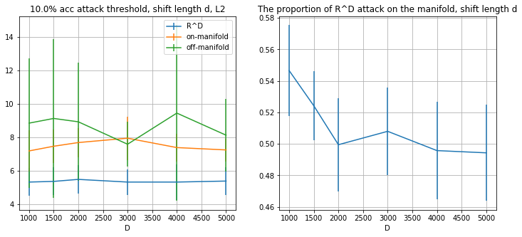
Figure 13: Attack strength threshold associating with $10\%$ robust test accuracy (left) and the on-manifold proportion in $\mathbb{R}^{D}$ attack when changing $d$. The optimizer takes weight_decay as 0.1. The number of epochs is changed to 500 in this experiment to save the computation time for large $D$ cases. Since we change the number of epochs in this experiment, we also conduct experiment for the scenario of Figure 3, and there is no change in the result.

D.2 MNIST

D.2.1 Architecture and training setting

We use Adam optimizer with learning rate $10^{-3}$ to train the model. The batch size is 256.

Layer
Conv2d(1, 16, 4, stride=2, padding=1), ReLU
Conv2d(16, 32, 4, stride=2, padding=1), ReLU
Linear(32*(7+$P/2$)*(7+$P/2$),100), ReLU
Linear(100, 10)

Table 6: Neural network architecture.

We take 0.02 as the stopping criteria because when $P=0$, the training loss is around 0.02 after 10 epochs. We repeat the experiment 30 times to get a mean and standard deviation.

D.2.2 Additional Figures

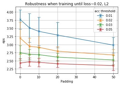
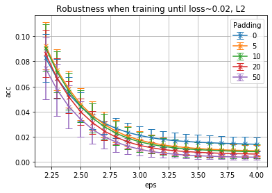
Figure 14: The relationship between attack strength and the padding number $P$ in Table 6 (left) and the relationship between robust test accuracy and attack strength under different $P$. $\ell_{2}$ attack. Train loss is 0.02.

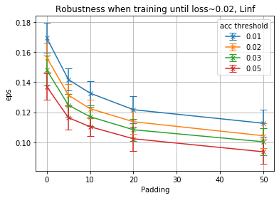
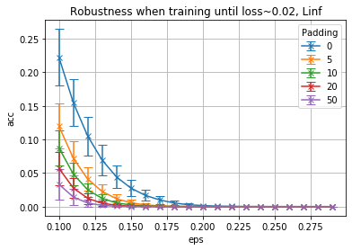
Figure 15: The relationship between attack strength and the padding number $P$ in Table 6 (left) and the relationship between robust test accuracy and attack strength under different $P$. $\ell_{\infty}$ attack. Train loss is 0.02.

References

- Adler and Taylor (2007) Adler, R. J. and Taylor, J. E. (2007), “Gaussian inequalities,” Random Fields and Geometry, 49–64.
- Bartlett et al. (2021) Bartlett, P., Bubeck, S., and Cherapanamjeri, Y. (2021), “Adversarial examples in multi-layer random relu networks,” Advances in Neural Information Processing Systems, 34, 9241–9252.
- Bubeck et al. (2021) Bubeck, S., Cherapanamjeri, Y., Gidel, G., and Tachet des Combes, R. (2021), “A single gradient step finds adversarial examples on random two-layers neural networks,” Advances in Neural Information Processing Systems, 34, 10081–10091.
- Carlini and Wagner (2017) Carlini, N. and Wagner, D. (2017), “Towards evaluating the robustness of neural networks,” in 2017 ieee symposium on security and privacy (sp), Ieee, pp. 39–57.
- Daniely and Shacham (2020) Daniely, A. and Shacham, H. (2020), “Most ReLU Networks Suffer from \ell^2 Adversarial Perturbations,” in Advances in Neural Information Processing Systems, eds. Larochelle, H., Ranzato, M., Hadsell, R., Balcan, M., and Lin, H., Curran Associates, Inc., vol. 33, pp. 6629–6636.
- Deng et al. (2009) Deng, J., Dong, W., Socher, R., Li, L.-J., Li, K., and Fei-Fei, L. (2009), “ImageNet: A large-scale hierarchical image database,” in 2009 IEEE Conference on Computer Vision and Pattern Recognition, pp. 248–255.
- Facco et al. (2017) Facco, E., d’Errico, M., Rodriguez, A., and Laio, A. (2017), “Estimating the intrinsic dimension of datasets by a minimal neighborhood information,” Scientific Reports, 7.
- Frei et al. (2023) Frei, S., Vardi, G., Bartlett, P. L., and Srebro, N. (2023), “The Double-Edged Sword of Implicit Bias: Generalization vs. Robustness in ReLU Networks,” arXiv preprint arXiv:2303.01456.
- Fukunaga and Olsen (1971) Fukunaga, K. and Olsen, D. (1971), “An Algorithm for Finding Intrinsic Dimensionality of Data,” IEEE Transactions on Computers, C-20, 176–183.
- Goodfellow et al. (2014) Goodfellow, I. J., Shlens, J., and Szegedy, C. (2014), “Explaining and harnessing adversarial examples,” arXiv preprint arXiv:1412.6572.
- Haro et al. (2008) Haro, G., Randall, G., and Sapiro, G. (2008), “Translated Poisson Mixture Model for Stratification Learning,” International Journal of Computer Vision, 80, 358–374.
- He et al. (2015) He, K., Zhang, X., Ren, S., and Sun, J. (2015), “Delving deep into rectifiers: Surpassing human-level performance on imagenet classification,” in Proceedings of the IEEE international conference on computer vision, pp. 1026–1034.
- He et al. (2016) — (2016), “Deep Residual Learning for Image Recognition,” in Proceedings of the IEEE Conference on Computer Vision and Pattern Recognition (CVPR).
- Hornik et al. (1989) Hornik, K., Stinchcombe, M., and White, H. (1989), “Multilayer feedforward networks are universal approximators,” Neural networks, 2, 359–366.
- James et al. (2013) James, G., Witten, D., Hastie, T., Tibshirani, R., et al. (2013), An introduction to statistical learning, vol. 112, Springer.
- Laurent and Massart (2000) Laurent, B. and Massart, P. (2000), “Adaptive estimation of a quadratic functional by model selection,” Annals of statistics, 1302–1338.
- LeCun et al. (2010) LeCun, Y., Cortes, C., and Burges, C. (2010), “MNIST handwritten digit database,” ATT Labs [Online]. Available: http://yann.lecun.com/exdb/mnist, 2.
- Ledoux (2006) Ledoux, M. (2006), “Isoperimetry and Gaussian analysis,” Lectures on Probability Theory and Statistics: Ecole d’Eté de Probabilités de Saint-Flour XXIV—1994, 165–294.
- Leshno et al. (1993) Leshno, M., Lin, V. Y., Pinkus, A., and Schocken, S. (1993), “Multilayer feedforward networks with a nonpolynomial activation function can approximate any function,” Neural networks, 6, 861–867.
- Liu et al. (2019) Liu, J., Bai, Y., Jiang, G., Chen, T., and Wang, H. (2019), “Understanding Why Neural Networks Generalize Well Through GSNR of Parameters,” in International Conference on Learning Representations.
- Lyu and Li (2020) Lyu, K. and Li, J. (2020), “Gradient Descent Maximizes the Margin of Homogeneous Neural Networks,” .
- Madry et al. (2017) Madry, A., Makelov, A., Schmidt, L., Tsipras, D., and Vladu, A. (2017), “Towards deep learning models resistant to adversarial attacks,” arXiv preprint arXiv:1706.06083.
- Melamed et al. (2023) Melamed, O., Yehudai, G., and Vardi, G. (2023), “Adversarial Examples Exist in Two-Layer ReLU Networks for Low Dimensional Data Manifolds,” arXiv preprint arXiv:2303.00783.
- Pinkus (1999) Pinkus, A. (1999), “Approximation theory of the MLP model in neural networks,” Acta numerica, 8, 143–195.
- Schmidt et al. (2018) Schmidt, L., Santurkar, S., Tsipras, D., Talwar, K., and Madry, A. (2018), “Adversarially robust generalization requires more data,” Advances in neural information processing systems, 31.
- Shamir et al. (2022) Shamir, A., Melamed, O., and BenShmuel, O. (2022), “The Dimpled Manifold Model of Adversarial Examples in Machine Learning,” .
- Szegedy et al. (2013) Szegedy, C., Zaremba, W., Sutskever, I., Bruna, J., Erhan, D., Goodfellow, I., and Fergus, R. (2013), “Intriguing properties of neural networks,” arXiv preprint arXiv:1312.6199.
- Vardi et al. (2022) Vardi, G., Yehudai, G., and Shamir, O. (2022), “Gradient methods provably converge to non-robust networks,” Advances in Neural Information Processing Systems, 35, 20921–20932.
- Xiao et al. (2017) Xiao, H., Rasul, K., and Vollgraf, R. (2017), “Fashion-MNIST: a Novel Image Dataset for Benchmarking Machine Learning Algorithms,” .
- Xiao et al. (2022) Xiao, J., Yang, L., Fan, Y., Wang, J., and Luo, Z.-Q. (2022), “Understanding adversarial robustness against on-manifold adversarial examples,” arXiv preprint arXiv:2210.00430.
- Zhang et al. (2022) Zhang, W., Zhang, Y., Hu, X., Goswami, M., Chen, C., and Metaxas, D. N. (2022), “A Manifold View of Adversarial Risk,” in International Conference on Artificial Intelligence and Statistics, PMLR, pp. 11598–11614.