Confidence on the Focal: Conformal Prediction
with Selection-Conditional Coverage

Abstract

Conformal prediction builds marginally valid prediction intervals that cover the unknown outcome of a randomly drawn new test point with a prescribed probability. However, a common scenario in practice is that, after seeing the data, practitioners decide which test unit(s) to focus on in a data-driven manner and seek for uncertainty quantification of the focal unit(s). In such cases, marginally valid conformal prediction intervals may not provide valid coverage for the focal unit(s) due to selection bias. This paper presents a general framework for constructing a prediction set with finite-sample exact coverage conditional on the unit being selected by a given procedure. The general form of our method works for arbitrary selection rules that are invariant to the permutation of the calibration units, and generalizes Mondrian Conformal Prediction to multiple test units and non-equivariant classifiers. We then work out the computationally efficient implementation of our framework for a number of realistic selection rules, including top-K selection, optimization-based selection, selection based on conformal p-values, and selection based on properties of preliminary conformal prediction sets. The performance of our methods is demonstrated via applications in drug discovery and health risk prediction.

1 Introduction

Conformal prediction is a versatile framework for quantifying the uncertainty of any black-box prediction model, by issuing a prediction set that covers the unknown outcome with a prescribed probability. Formally, suppose the task is to predict an outcome $Y\in{\mathcal{Y}}$ based on features $X\in{\mathcal{X}}$. Given a set of calibration data $\{(X_{i},Y_{i})\}_{i=1}^{n}$ and the features of a new test point $X_{n+1}$, conformal prediction builds upon a given prediction model and delivers a prediction set $\widehat{C}_{\alpha,n+1}\subseteq{\mathcal{Y}}$ at level $\alpha\in(0,1)$, which obeys

$$\mathbb{P}\big{(}Y_{n+1}\in\widehat{C}_{\alpha,n+1}\big{)}\geq 1-\alpha,$$ (1)

as long as $\{(X_{i},Y_{i})\}_{i=1}^{n+1}$ are exchangeable (e.g., when they are i.i.d. samples). The probability in (1) is over both the calibration data and the test point (Vovk et al.,, 2005; Lei et al.,, 2018).

With this finite-sample, distribution-free guarantee, the conformal prediction set $\widehat{C}_{\alpha,n+1}$ describes a range of plausible values the unknown outcome $Y_{n+1}$ may take, thereby expected to inform downstream decision-making based on the black-box prediction model. With such a promise, methods for constructing marginally valid – in the sense of (1) – prediction sets have been developed for various problems; see e.g., Angelopoulos and Bates, (2021) for a review.

In many downstream applications, however, people are often only interested in a selective subset of units. Practitioners may act upon a unit if it exhibits an interesting property (Olsson et al.,, 2022; Sokol et al.,, 2024; Levitskaya,, 2023). In other cases, they may focus on a subset of test units picked by a complicated data-dependent process such as resource optimization (Svensson et al.,, 2018; Castro and Petrovic,, 2012; Kemper et al.,, 2014; Gocgun and Puterman,, 2014). It would be misleading for the practitioners if the prediction sets fail to deliver the promised coverage guarantee for the selected unit(s). Let us discuss a few applications where such cases may arise.

• In drug discovery, an important task is to predict the binding affinity of a drug candidate to a disease target, which informs subsequent drug prioritization (Laghuvarapu et al.,, 2024). Among many drug candidates, scientists may only focus on those with highest predicted affinites, or those selected by a false discovery rate (FDR)-controlling procedure (Jin and Candès, 2023b, ), or whose prediction sets only cover high values (Svensson et al.,, 2017), or those optimizing resource usage (Svensson et al.,, 2018). It may lead to a waste of resources if more than an $\alpha$-fraction of the prediction sets for the selected drugs fail to cover the actual binding affinities.

• In business decision-making, companies may take different inventory decisions based on whether a conformal prediction set suggests a strong demand or a weak demand (Levitskaya,, 2023). Similarly, it will be problematic if the average coverage among strong-demand predictions is below $1-\alpha$.

• In disease diagnosis, Olsson et al., (2022) suggest human intervention if the prediction set for a disease status is too large (this implicitly declares confidence in small prediction sets; see similar ideas in Ren et al., (2023); Sokol et al., (2024)). However, it would be concerning if more than an $\alpha$-fraction of small-sized prediction sets – “approved” as confident – miss the true disease status.

• In healthcare management, patients may be sent to different healthcare categories based a program that optimizes some performance measure (such as waiting time) subject to certain constraints, such as budget, capacity, or fairness (Castro and Petrovic,, 2012; Kemper et al.,, 2014; Gocgun and Puterman,, 2014). The subset of patients in each category is therefore data-dependent.

In all these examples, it is highly desirable that a prediction set should cover the unknown outcome for a unit of interest with a prescribed probability. This motivates a stronger, selection-conditional guarantee. Supposing there are $m\geq 1$ test units ${\mathcal{D}}_{\textnormal{test}}=\{X_{n+j}\}_{j=1}^{m}$, we shall aim for

$$\mathbb{P}\big{(}Y_{n+j}\in\widehat{C}_{\alpha,n+j}{\,|\,}j\in{\mathcal{S}}({\mathcal{D}}_{\textnormal{calib}},{\mathcal{D}}_{\textnormal{test}})\big{)}\geq 1-\alpha,$$ (2)

where ${\mathcal{D}}_{\textnormal{calib}}=\{(X_{i},Y_{i})\}_{i=1}^{n}$ is the calibration data, and ${\mathcal{S}}(\cdot,\cdot)$ is a data-driven process to decide which units are of interest, which maps the calibration and test data to a subset of $\{1,\dots,m\}$. Our target is similar in spirit to the post-selection inference (Lee et al.,, 2016; Markovic et al.,, 2017; Tibshirani et al.,, 2018), but we consider predictive inference settings and develop distinct techniques; see Section 1.3 for more discussion. Throughout, we focus on settings where the prediction sets are constructed after ${\mathcal{S}}({\mathcal{D}}_{\textnormal{calib}},{\mathcal{D}}_{\textnormal{test}})$ is determined. By separating the selection process from the (post hoc) uncertainty quantification step, we leave the freedom of defining selection rules to the practitioners.

A prediction set with marginal validity (1) does not necessarily cover an unknown outcome conditional on being of interest as in (2). Such a selection issue has recently been raised in the literature of predictive inference: through analysis of a real drug discovery dataset, Jin and Candès, 2023b (, Section 1) demonstrate that more than $30\%$ of seemingly promising prediction sets (in the sense that $\widehat{C}_{\alpha,n+j}=\{\text{active}\}$) miss the actual outcomes when the nominal marginal miscoverage rate is $\alpha=0.01$. We shall see more examples of this issue in our numerical experiments with various selection processes. New techniques are therefore needed for constructing prediction sets achieving (2).

1.1 Exchangeability via reference set

Accounting for selection in conformal prediction is a delicate task since it breaks exchangebility. The core of conformal prediction is to leverage the exchangeability among the calibration and test data, such that their “prediction residuals”, referred to as nonformormity scores, are comparable in distribution (see Section 3.1 for more details). The calibration scores therefor inform the magnitude of uncertainty in a new test point (Vovk et al.,, 2005). However, given a selection event, the calibration data are not exchangeable with a test point any more, leading to the violation of coverage guarantee mentioned above. In general, the selection-conditional distributions of these scores are intricate since the selection event can be highly data-dependent.

Such a challenge motivates our new framework, named JOint Mondrian Conformal Inference (JOMI), which builds prediction sets that achieve selection-conditional coverage, with (2) as a special case. As visualized in Figure 1, our key idea is to find a “reference set”, a data-dependent subset of calibration data that remain exchangeable with respect to a new test point conditional on the selection event. This reference set thus provides calibrated quantification of uncertainty for a selected unit. The mechanism we devise works generally for arbitrary selection rules ${\mathcal{S}}({\mathcal{D}}_{\textnormal{calib}},{\mathcal{D}}_{\textnormal{test}})$ that are invariant to permutations of data in ${\mathcal{D}}_{\textnormal{calib}}$, and can be computed efficiently for a wide range of commonly used selection rules.

Figure 1: Visualization of the intuition of the reference set. (a) Marginally, the calibration data (black) are exchangeable with respect to the test point (blue). (b) The calibration data are not exchangeable with respect to the test point (shaded blue) given a selection event. (c) We find calibration data which, when posited as a “test point”, would lead to the same selection event. (d) The reference set consists of calibration data that are exchangeable with respect to the test point given selection, and we use them to construct JOMI prediction sets.

We also note that the selection-conditional coverage (2) may be implied by other stronger notions such as conditional coverage: $\mathbb{P}(Y_{n+1}\in\widehat{C}_{\alpha,n+1}{\,|\,}X_{n+1}=x)\geq 1-\alpha$ for $\mathbb{P}$-almost all $x\in{\mathcal{X}}$. Conditional coverage implies (2) if $\{(X_{i},Y_{i})\}_{i=1}^{n+1}$ are mutually independent and the selection rule only depends on test features. However, it is not achievable by finite-length prediction intervals without distributional assumptions (Vovk et al.,, 2005; Barber et al.,, 2021), and practical selection rules may also depend on other information. Given these considerations, we may view (2) as a “relaxed” version of conditional coverage that is both achievable and relevant for practical use.

1.2 Preview of contributions

In Section 3, we introduce the general formulation of JOMI, including the construction of reference set and its use in deriving a selection-conditionally valid prediction set. We prove that when ${\mathcal{D}}_{\textnormal{calib}}$ and $(X_{n+j},Y_{n+j})$ are (marginally) exchangeable, the prediction set $\widehat{C}_{\alpha,n+j}$ produced by JOMI covers $Y_{n+j}$ with probability at least $1-\alpha$ conditional on a selection event. The selection event can be “test unit $j$ is selected”, which leads to (2); it can also be more granular, such as “test unit $j$ is selected, and there are $k$ selected test units”. This framework is valid for any selection rule ${\mathcal{S}}({\mathcal{D}}_{\textnormal{calib}},{\mathcal{D}}_{\textnormal{test}})$ that is permutation-invariant to ${\mathcal{D}}_{\textnormal{calib}}$, without any modeling assumptions on the data generating process.

In Section 4, we study the computational aspect of JOMI. In particular, we show that when $|{\mathcal{Y}}|<\infty$, our framework can be efficiently implemented within a computational complexity of $O(|{\mathcal{Y}}|mn)$ times that of the selection rule. We also work out efficient implementation of JOMI for a number of selection processes that may be of practical interest, including:

• Covariate-dependent selection. When the selection rule does not involve $\{Y_{i}\}_{i=1}^{n}$, the computation complexity of our generic method is (at most) $O(mn)$ times that of the selection rule. This implies efficient implementation for a wide range of problems, including various forms of top-K selection and selection based on complicated constrained optimization programs. As a special case, we recover the method of Bao et al., (2024) for top-K selection among test data, and provide valid solutions to other ranking-based selection methods attempted in their work.

• Conformal p-value-based selection. We derive efficient implementation for selection rules based on conformal p-values with both fixed and data-dependent thresholds. For instance, our prediction set is finite-sample exactly valid for units selected by Conformalized Selection (Jin and Candès, 2023b, ), which is studied in Bao et al., (2024) with approximate FCR guarantee.

• Selection based on preliminary conformal prediction sets. In addition, we derive a general, efficient instantiation when selecting units whose marginal prediction sets demonstrate certain interesting properties, such as being of a short length, or having a lower bound above a threshold. Our methods can be useful for re-calibrating the uncertainty quantification of such seemingly promising units.

Finally, we demonstrate the application of our methods via several realistic selection rules that may occur in drug discovery (Section 5) and health risk prediction (Section 6). Our results show that marginal prediction sets may undercover or overcover the selected units, while our methods always achieve the promised coverage guarantees.

1.3 Related work

Our method extends conformal prediction, which is a general framework for building marginally valid prediction intervals (Vovk et al.,, 2005; Lei et al.,, 2018; Romano et al.,, 2019, 2020). Compared with vanilla conformal prediction, we aim at selection-conditional coverage for a unit of interest, instead of marginal coverage for an “average” unit. Particularly related to our framework is Mondrian Conformal Prediction (MCP) (Vovk et al.,, 2003), which uses a subset of calibration data to build a prediction set with coverage conditional on a pre-determined or permutation-equivariant class membership. Achieving selection-conditional coverage is a new goal with distinct motivations from MCP. Moreover, our techniques and scopes of application are significantly different from those of MCP (see Remark 1).

The selection-conditional guarantee we seek for is closely related to the post-selection inference (POSI) literature (Berk et al.,, 2013; Tibshirani et al.,, 2016; Chernozhukov et al.,, 2015) and in particular conditional selective inference (Lee et al.,, 2016; Markovic et al.,, 2017; Reid et al.,, 2017; Tibshirani et al.,, 2018; Kivaranovic and Leeb,, 2020; McCloskey,, 2024). In POSI, one important task is to build confidence intervals for selected model parameters conditional on a selection event, which is close to our selection-conditional coverage guarantee. Methods for this goal usually leverage specific problem structures such as linearity and distribution of the estimators (Zhong and Prentice,, 2008; Lee et al.,, 2016; Tian and Taylor,, 2017; Andrews et al.,, 2024; Liu,, 2023). As we focus on predictive inference (where the inferential targets are random variables instead of parameters), we leverage the exchangeability across units to achieve exact selection-conditional coverage, and thus our method substantially differs from POSI.

Another related error notion in the selective inference literature is the false coverage rate (FCR) (Benjamini and Yekutieli,, 2005), which is defined as the expected fraction of selected objects not covered by their confidence/prediction sets. We provide a detailed comparison between FCR and selection-conditional coverage in Section 2.2. Methods for achieving FCR control have been proposed for various settings (Benjamini and Yekutieli,, 2005; Weinstein et al.,, 2013; Weinstein and Ramdas,, 2020; Zhao and Cui,, 2020; Xu et al.,, 2022). In particular, Weinstein and Ramdas, (2020) introduce an online FCR-controlling method that can be applied to conformal prediction with selection. They consider sequentially arriving test units, and require the selection of a current unit to only depend on its prediction set and past selection decisions. In contrast, we allow the selection rule to simultaneously depend on all test units, such as top-K selection, optimization-based selection, and conformal p-value-based selection. Our approach to error control differs from theirs as well: while they achieve FCR control by adjusting the confidence level of marginal prediction sets, we leverage a judiciously chosen subset of calibration data to construct post-selection prediction sets with selection-conditional coverage. Another closely related work is Bao et al., (2024) who study prediction sets for selected units with (approximate) FCR control, yet they achieve exact guarantee only for a limited class of selection rules such as top-K selection. Later on, we will show that JOMI yields the same prediction sets as theirs when applied to top-K selection, and leads to exact guarantee for other problems they addressed with approximate FCR control. It also applies to many more settings with complicated selection rules that cannot be handled by their methods. Finally, a concurrent work of Gazin et al., (2024) (which was posted shortly after the first appearance of this work on arXiv) also studies the selective inference problem in conformal prediction. It specifically considers selection based on properties of prediction sets, but jointly calibrates the selection procedure and the construction of prediction sets while achieving FCR control. In contrast, we take a complementary perspective, decoupling the selection step and the uncertainty quantification step, which allows the development of a versatile framework that is applicable to a broader range of selection rules.

More broadly, many recent works have studied selective inference problems in conformal prediction, mostly focusing on multiple testing, i.e., selecting individuals that obey some properties with FDR control. This includes selecting outliers (Bates et al.,, 2023; Marandon et al.,, 2022; Liang et al.,, 2022; Bashari et al.,, 2024) and selecting high-quality data (Jin and Candès, 2023b, ; Jin and Candès, 2023a, ). The construction of conformal prediction sets is an orthogonal direction, and our methods also work for selection based on such procedures; see Section 4.2.2 for an efficient method.

Under a similar name, Sarkar and Kuchibhotla, (2023) propose “post-selection inference for conformal prediction”, but they mainly focus on selecting the confidence level $\alpha\in(0,1)$ instead of selecting the units. In addition, they are closer to the “simultaneous inference” strand in POSI since they aim for valid inference simultaneously for all confidence levels, other than conditional on a selection event. For these reasons, our methods and guarantees are quite different.

Notations.

We close this section by introducing several notations that will be used throughout the paper. For a positive integer $n\in\mathbb{N}^{+}$, we write $[n]:=\{1,\dots,n\}$. For convenience, we write the data pair $Z=(X,Y)$, so that the calibration data is ${\mathcal{D}}_{\textnormal{calib}}=\{Z_{i}\}_{i=1}^{n}$. For any $j\in[m]$, we define the augmented calibration set ${\mathcal{D}}_{j}={\mathcal{D}}_{\textnormal{calib}}\cup\{Z_{n+j}\}$ and the remaining test set ${\mathcal{D}}^{c}_{j}={\mathcal{D}}_{\textnormal{test}}\backslash\{X_{n+j}\}$. The unordered set of ${\mathcal{D}}_{j}$ is denoted as $[{\mathcal{D}}_{j}]=[Z_{1},\dots,Z_{n},Z_{n+j}]$, which provides the order statistics but not the ordering.

2 Problem setup

Following the split conformal prediction framework (Vovk et al.,, 2005; Lei et al.,, 2018), we are to build our prediction sets based on a prediction model fitted on a training set ${\mathcal{D}}_{\textnormal{train}}$. We assume ${\mathcal{D}}_{\textnormal{train}}$ is independent of the calibration and test data. In what follows, we always condition on ${\mathcal{D}}_{\textnormal{train}}$, thereby treating the fitted models as fixed. In this section, we discuss the selection-conditional coverage guarantees we study in this paper and compare them to other related notions in the literature.

2.1 Selection-conditional coverage

Recall that $j\in[m]$ is a focal unit if $j\in\widehat{\mathcal{S}}$, where $\widehat{\mathcal{S}}={\mathcal{S}}({\mathcal{D}}_{\textnormal{calib}},{\mathcal{D}}_{\textnormal{test}})\subseteq[m]$ is obtained from a selection rule ${\mathcal{S}}$ that depends on the observed data. Its potential dependence on ${\mathcal{D}}_{\textnormal{train}}$ is clear since we treat ${\mathcal{D}}_{\textnormal{train}}$ as fixed. Without loss of generality, we posit that ${\mathcal{S}}$ is a deterministic function; when the selection rule is randomized, one can condition on its randomness and follow our framework.

For each test unit $j$, we wish to construct a prediction set $\widehat{C}_{\alpha,n+j}\subseteq{\mathcal{Y}}$ such that

$$\mathbb{P}\big{(}Y_{n+j}\in\widehat{C}_{\alpha,n+j}\,\big{|}\,j\in\widehat{\mathcal{S}},\leavevmode\nobreak\ \widehat{\mathcal{S}}\in\mathfrak{S}\big{)}\geq 1-\alpha,$$ (3)

where $\alpha\in(0,1)$ is the confidence level, and $\mathfrak{S}\subseteq 2^{[m]}$ is some pre-specified collection of subsets of $[m]$. We call $\mathfrak{S}$ the selection taxonomy in what follows.

In Equation (3), difference choices of $\mathfrak{S}$ leads to a spectrum of granularity in the conditioning event. For instance, taking $\mathfrak{S}=\{S_{0}\}$ for some $S_{0}\subseteq[m]$ achieves coverage conditional on selecting a specific set; this is similar to the coverage guarantee in Lee et al., (2016) for high-dimensional parameter inference. Taking $\mathfrak{S}=\{S\subseteq[m]\colon|S|=r\}$ for some $r\leq m$ achieves coverage conditional on selecting a specific number of units. Finally, taking $\mathfrak{S}=2^{[m]}$ puts no restrictions on the selection set, giving rise to the guarantee (2) introduced in the beginning, that is, coverage conditional on a unit being selected.

2.2 Relations among notions of selective coverage

Before introducing our methods, we take a moment here to compare different notions of selective coverage. Readers who are more interested in our methodology may skip the remaining of this section.

Our first observation is that (3) implies (2) under appropriate conditions. The proof of the next proposition is in Appendix B.1.

Proposition 1.

If $\widehat{C}_{\alpha,n+j}$ satisfies (3) for a set of mutually disjoint taxonomies $\{\mathfrak{S}_{\ell}\}_{\ell\in{\mathcal{L}}}$ such that $\cup_{\ell\in{\mathcal{L}}}\mathfrak{S}_{\ell}=2^{[m]}$, then it satisfies (2).

To distinguish the selection-conditional coverage in (3) and that in (2), we refer to the former as strong selection-conditional coverage and the latter as weak selection-conditional coverage.

Another widely used post-selection-type guarantee is the false coverage rate (FCR) (Benjamini and Yekutieli,, 2005), defined as the expected proportion of selected units missed by the prediction set:

$$\text{FCR}\,:=\,\mathbb{E}\bigg{[}\frac{\sum_{j\in[m]}\mathds{1}\{j\in\widehat{{\mathcal{S}}},Y_{n+j}\notin\widehat{C}_{\alpha,n+j}\}}{|\widehat{{\mathcal{S}}}|\vee 1}\bigg{]},$$ (4)

where $a\vee b=\max\{a,b\}$ for any $a,b\in\mathbb{R}$. As introduced earlier, Weinstein and Ramdas, (2020) and Bao et al., (2024) mainly focus on constructing prediction sets with FCR control. However, with $m=1$, it holds that $\text{FCR}=\mathbb{P}(j\in\widehat{{\mathcal{S}}},Y_{n+j}\notin\widehat{C}_{\alpha}(X_{n+j}))\leq\alpha$ for any marginally valid prediction set. Thus, FCR does not address the selection issue when we consider one test point.

We claim that the strong selection-conditional coverage implies FCR control with a proper choice of the selection taxonomy. The proof of the following proposition can be found in Appendix B.2.

Proposition 2.

Suppose $\widehat{C}_{\alpha,n+j}$ satisfies the strong selection-conditional coverage (3) for a class of mutually disjoint selection taxonomies $\{\mathfrak{S}_{\ell}\}_{\ell\in{\mathcal{L}}}$ such that $\cup_{\ell\in{\mathcal{L}}}\mathfrak{S}_{\ell}=2^{[m]}$, and for each $\ell\in{\mathcal{L}}$, $\mathfrak{S}_{\ell}\subseteq\{S\subseteq[m]\colon|S|=r(\ell)\}$ for some $0\leq r(\ell)\leq m$. Then its false coverage rate (4) is upper bounded by $\alpha\cdot\mathbb{P}(\widehat{C}_{\alpha,n+j}\neq\varnothing)\leq\alpha$.

As a side note, we find that the weak selection-conditional coverage does not necessarily imply FCR control, although in some special cases both can be true (see, e.g., Bao et al., (2024) for such examples). We put this as a proposition below, with a counterexample given in Appendix B.3.

Proposition 3.

There exists an instance and prediction sets $\{\widehat{C}_{\alpha,n+j}:j\in\widehat{{\mathcal{S}}}\}$ such that $\{\widehat{C}_{\alpha,n+j}:j\in\widehat{{\mathcal{S}}}\}$ satisfy the weak selection-conditional coverage at level $\alpha$ but violate the FCR control at level $\alpha$.

3 JOMI: a unified framework

3.1 Warm-up: split conformal prediction

To warm up, we briefly summarize the split conformal prediction (SCP) method (Vovk et al.,, 2005; Lei et al.,, 2018) and how it achieves finite-sample coverage under exchangeability.

SCP starts with a nonconformity score function $V\colon{\mathcal{X}}\times{\mathcal{Y}}\mapsto\mathbb{R}$ determined by ${\mathcal{D}}_{\textnormal{train}}$, so that $V(x,y)$ informs how well a hypothetical value $y\in{\mathcal{Y}}$ conforms to a machine prediction. For instance, one may set $V(x,y)=|y-\widehat{\mu}(x)|$, where $\widehat{\mu}(x)$ is regression function fitted on ${\mathcal{D}}_{\textnormal{train}}$. Other popular choices include CQR (Romano et al.,, 2019) for regression and APS (Romano et al.,, 2020) for classification.

Compute $V_{i}=V(X_{i},Y_{i})$ for $i\in[n]$. The split conformal prediction set for test unit $j\in[m]$ is

$$\widehat{C}_{\alpha,n+j}^{\text{SCP}}=\Big{\{}y\colon V(X_{n+j},y)\leq\text{Quantile}\big{(}1-\alpha;\{V_{i}\}_{i=1}^{n}\cup\{+\infty\}\big{)}\Big{\}},$$ (5)

where $\text{Quantile}(1-\alpha;\cdot)$ is the $(1-\alpha)$-th empirical quantile of the set in the second argument. When $(Z_{1},\dots,Z_{n},Z_{n+j})$ are exchangeable, $\widehat{C}_{\alpha,n+j}^{\text{SCP}}$ achieves valid marginal coverage (1) (Vovk et al.,, 2005).

It helps motivate our approach to see the ideas behind the validity of $\widehat{C}_{\alpha,n+j}^{\text{SCP}}$. In words, $\widehat{C}_{\alpha,n+j}^{\text{SCP}}$ finds hypothesized values of $y$ that make $V(X_{n+j},y)$ look similar to calibration scores. Note that

$$\mathbb{P}\big{(}Y_{n+j}\in\widehat{C}_{\alpha,n+j}^{\text{SCP}}\big{)}=\mathbb{P}\Big{(}V_{n+j}\leq\text{Quantile}\big{(}1-\alpha;\{V_{i}\}_{i=1}^{n}\cup\{V_{n+j}\}\big{)}\Big{)},$$ (6)

where $V_{n+j}=V(X_{n+j},Y_{n+j})$. Recall the unordered set $[{\mathcal{D}}_{j}]=[Z_{1},\dots,Z_{n},Z_{n+j}]$ where $Z_{i}=(X_{i},Y_{i})$. Conditional on the event $\{[{\mathcal{D}}_{j}]=[z_{1},\dots,z_{n+j}]\}$, the only randomness is in the ordering of $(Z_{1},\dots,Z_{n+j})$; due to exchangeability, the probability of $Z_{n+j}$ taking on each value in $z_{1},\dots,z_{n},z_{n+j}$ is equal. Therefore, conditional on $[{\mathcal{D}}_{j}]=[z_{1},\dots,z_{n+j}]$, the chance of $V_{n+j}$ being no greater than the $(1-\alpha)$-th quantile of $[v_{1},\dots,v_{n},v_{n+j}]$, where $v_{i}=v(z_{i})$, is at least $1-\alpha$, i.e.,

$$\mathbb{P}\Big{(}V_{n+j}\leq\text{Quantile}\big{(}1-\alpha;\{v_{i}\}_{i=1}^{n}\cup\{v_{n+j}\}\big{)}\,\Big{|}\,[{\mathcal{D}}_{j}]=[z_{1},\dots,z_{n+j}]\Big{)}\geq 1-\alpha.$$ (7)

This leads to (6) by the tower property. Therefore, inverting the criterion on the right-hand side of (6) gives a valid prediction set for $Y_{n+j}$.

The reason why vanilla SCP may fail to achieve selection-conditional coverage like (3) is that, conditional on the selection event, the data points $\{Z_{1},\dots,Z_{n},Z_{n+j}\}$ are no longer exchangeable. In other words, in (7), it is unclear how $V_{n+j}$ is distributed over $v_{1},\dots,v_{n+j}$ if we additionally condition on the selection event. As such, a natural remedy is to find a subset of calibration data that are “exchangeable” with respect to the test point after conditioning on the selection event, and leverage their scores to calibrate the prediction of the test unit. We introduce our methods in the next.

3.2 Conformal inference via a reference set

Fix a test unit $j\in[m]$. Recall that $Z_{n+j}(y)=(X_{n+j},y)$ is the imputed test point with a hypothesized response $y\in{\mathcal{Y}}$. The core of our method is to find calibration points that are exchangeable with respect to the test point conditional on the selection set. At a high level, they are calibration units $i\in[n]$ that are “indistinguishable” with $j\in[m]$, in the sense that treating $Z_{n+j}(y)$ as a calibration point and $Z_{i}$ as a test point results in the same selection event.

We formalize this idea via a “swap” operation. For any calibration unit $i\in[n]$, we define the “swapped” calibration data ${\mathcal{D}}_{{\textnormal{calib}}}^{{\textnormal{swap}(i,j)}}(y)$ and the swapped test data ${\mathcal{D}}_{{\textnormal{test}}}^{{\textnormal{swap}(i,j)}}$ as follows:

$${\mathcal{D}}_{{\textnormal{calib}}}^{{\textnormal{swap}(i,j)}}(y)=(Z_{1}^{{\textnormal{swap}(i,j)}}(y),Z_{2}^{{\textnormal{swap}(i,j)}}(y),\dots,Z_{n}^{{\textnormal{swap}(i,j)}}(y)),$$

$${\mathcal{D}}_{{\textnormal{test}}}^{{\textnormal{swap}(i,j)}}=(X_{n+1}^{{\textnormal{swap}(i,j)}},X_{n+2}^{{\textnormal{swap}(i,j)}},\dots,X_{n+m}^{{\textnormal{swap}(i,j)}}),$$

where for $k\in[n]$ and $\ell\in[m]$,

$$Z_{k}^{{\textnormal{swap}(i,j)}}(y)=\begin{cases}Z_{n+j}(y)&k=i,\\ Z_{k}&k\neq i.\end{cases}\quad X_{n+\ell}^{{\textnormal{swap}(i,j)}}=\begin{cases}X_{i}&\ell=j,\\ X_{n+\ell}&\ell\neq j.\end{cases}$$

That is, ${\mathcal{D}}_{\textnormal{calib}}^{\textnormal{swap}(i,j)}(y)$ and ${\mathcal{D}}_{\textnormal{test}}^{\textnormal{swap}(i,j)}$ are the calibration and test data if we treat $Z_{i}$ as the $j$-th test point, and $Z_{n+j}(y)$ as the $i$-th calibration point. Figure 2 is an illustration of the swap operation.

Figure 2: Graphical illustration of ${\mathcal{D}}_{\textnormal{calib}}^{\textnormal{swap}(i,j)}(y)$ and ${\mathcal{D}}_{\textnormal{test}}^{{\textnormal{swap}(i,j)}}$.

Applying the same selection rule ${\mathcal{S}}$ to the swapped data, we define the swapped selection set with the hypothesized $y$ as

$$\widehat{\mathcal{S}}^{{\textnormal{swap}(i,j)}}(y)={\mathcal{S}}\big{(}{\mathcal{D}}_{{\textnormal{calib}}}^{{\textnormal{swap}(i,j)}}(y),{\mathcal{D}}_{{\textnormal{test}}}^{{\textnormal{swap}(i,j)}}\big{)}.$$

Then, we define the “reference set” for achieving (3) with taxonomy $\mathfrak{S}$ as

$$\widehat{{\mathcal{R}}}_{n+j}(y)=\big{\{}i\in[n]\colon j\in\widehat{\mathcal{S}}^{{\textnormal{swap}(i,j)}}(y),\text{ and }\widehat{{\mathcal{S}}}^{{\textnormal{swap}(i,j)}}(y)\in\mathfrak{S}\big{\}}.$$ (8)

In words, the reference set is the collection of calibration points $i\in[n]$ such that, after swapping unit $i$ and $n+j$, the test point $j$ remains in the focal set and the focal set remains in $\mathfrak{S}$. We use the notation $\widehat{{\mathcal{R}}}_{n+j}(y)$ to emphasize that $\widehat{\mathcal{R}}_{n+j}(\cdot)$ is a data-dependent mapping from ${\mathcal{Y}}$ to the power set of $[n]$.

With all the preparation, we define our prediction set for $Y_{n+j}$ as

$$\widehat{C}_{\alpha,n+j}=\Big{\{}y\in{\mathcal{Y}}\colon V(X_{n+j},y)\leq{\textnormal{Quantile}}\big{(}1-\alpha;\{V_{i}\}_{i\in\widehat{\mathcal{R}}_{n+j}(y)}\cup\{+\infty\}\big{)}\Big{\}}.$$ (9)

As we shall show shortly, our prediction set (9) achieves near-exact coverage when the nonconformity score is continuous and the reference set is of moderate size. In addition, we can achieve exact coverage by introducing extra randomness:

$$\widehat{C}_{\alpha,n+j}^{\textnormal{rand}}$$

$$\leavevmode\nobreak\ =\bigg{\{}y\colon\frac{\sum_{i\in\widehat{\mathcal{R}}_{n+j}(y)}\mathds{1}\{V(X_{n+j},y)<V_{i}\}+U_{j}\cdot(1+\sum_{i\in\widehat{\mathcal{R}}_{n+j}(y)}\mathds{1}\{V(X_{n+j},y)=V_{i}\})}{1+|\widehat{\mathcal{R}}_{n+j}(y)|}\leq 1-\alpha\bigg{\}},$$ (10)

where $U_{1},\ldots,U_{m}$ are i.i.d. random variables drawn from $\textrm{Unif}[0,1]$ that are independent of the data.

Remark 1 (Connection to MCP).

Our framework is closely related to Mondrian Conformal Prediction (MCP) (Vovk et al.,, 2003) which applies to case of one test unit ($m=1$). Given $K$ categories $[K]$, MCP assumes access to a classifier ${\mathcal{K}}$ that gives the class label for all units: $(\kappa_{1},\kappa_{2},\dots,\kappa_{n+1})={\mathcal{K}}(Z_{1},Z_{2},\dots,Z_{n+1}),$ where $\kappa_{i}\in[K]$ is the class label for unit $i$. The classifier ${\mathcal{K}}$ is required to be equivariant to any permutation $\pi$ of $[n+1]$, i.e., $(\kappa_{\pi(1)},\kappa_{\pi(2)},\dots,\kappa_{\pi(n+1)})={\mathcal{K}}(Z_{\pi(1)},Z_{\pi(2)},\dots,Z_{\pi(n+1)}).$ The goal of MCP is to construct a prediction set for a test unit with category-wise coverage, i.e., $\mathbb{P}(Y_{n+1}\in\widehat{C}^{\textnormal{MCP}}_{\alpha,n+1}{\,|\,}\kappa_{n+1}=k)$ for each $k\in[K]$. This is achieved by finding a subset of calibration data that are categorized as $k$ for each hypothesized test outcome $y\in{\mathcal{Y}}$, i.e.,

$$\widetilde{{\mathcal{R}}}(y)=\{i\in[n]:{\mathcal{K}}({\mathcal{D}}_{{\textnormal{calib}}},(X_{n+1},y))_{[i]}=k\},$$ (11)

and then constructing the prediction set as

$$\widehat{C}^{\textnormal{MCP}}_{\alpha,n+1}=\Big{\{}y\in{\mathcal{Y}}:V(X_{n+1},y)\leq{\textnormal{Quantile}}\big{(}1-\alpha;\{V_{i}\}_{i\in\widetilde{{\mathcal{R}}}(y)}\cup\{\infty\}\big{)}\Big{\}}.$$

While the setups seem different, JOMI effectively reduces to MCP when ${\mathcal{K}}$ is a binary classifier and ${\mathcal{S}}$ is equivariant under permutations of $[n+1]$. To see this, one can view the selection rule ${\mathcal{S}}$ as categorizing test points into two classes (selected or not selected), and selection-conditional coverage (3) as coverage given the “selected” category. In this way, one can check that our reference set $\widehat{{\mathcal{R}}}_{n+1}(y)$ coincides with $\widetilde{{\mathcal{R}}}(y)$ defined in (11), and thus the prediction sets also coincide.

With a distinct goal of selection-conditional coverage, we additionally address the challenge that realistic selection rules are often asymmetric to calibration and (multiple) test points. To this end, JOMI generalizes MCP via a more delicate framework for finding exchangeable subgroups. As we jointly consider the calibration and test points when defining the reference set, we call our method JOint Mondrian Conformal Inference (JOMI).

3.3 Theoretical guarantee

Theorem 1 confirms the conditional validity of our prediction sets $\widehat{C}_{\alpha,n+j}$ in (9) and $\widehat{C}^{\textnormal{rand}}_{\alpha,n+j}$ in (3.2).

Theorem 1.

Suppose ${\mathcal{S}}({\mathcal{D}}_{\textnormal{calib}},{\mathcal{D}}_{\textnormal{test}})$ is invariant to permutations of ${\mathcal{D}}_{\textnormal{calib}}$, and that $\{Z_{i}\}_{i=1}^{n}\cup\{Z_{n+j}\}$ are exchangeable conditional on $\{X_{n+\ell}\}_{\ell\in[m]\backslash\{j\}}$ for any $j\in[m]$. Then, for any selection taxonomy $\mathfrak{S}$, the following statements hold.

1. $\widehat{C}_{\alpha,n+j}$ defined in (9) obeys

   $$\mathbb{P}\big{(}Y_{n+j}\in\widehat{C}_{\alpha,n+j}\,\big{|}\,j\in\widehat{\mathcal{S}},\leavevmode\nobreak\ \widehat{\mathcal{S}}\in\mathfrak{S}\big{)}\geq 1-\alpha.$$ (12)

   Furthermore, if ties among $V_{1},\ldots,V_{n},V_{n+j}$ occur with probability zero, then

   $$\mathbb{P}\big{(}Y_{n+j}\in\widehat{C}_{\alpha,n+j}\,\big{|}\,j\in\widehat{\mathcal{S}},\leavevmode\nobreak\ \widehat{\mathcal{S}}\in\mathfrak{S}\big{)}\leq 1-\alpha+\mathbb{E}\bigg{[}\frac{1}{1+|\widehat{{\mathcal{R}}}_{n+j}(Y_{n+j})|}\bigg{]}.$$ (13)

2. The randomized prediction set $\widehat{C}_{\alpha,n+j}^{\textnormal{rand}}$ defined in (3.2) satisfies

   $$\mathbb{P}(Y_{n+j}\in\widehat{C}_{\alpha,n+j}^{\textnormal{rand}}{\,|\,}j\in\widehat{\mathcal{S}},\leavevmode\nobreak\ \widehat{{\mathcal{S}}}\in\mathfrak{S})=1-\alpha.$$

We defer the detailed proof of Theorem 1 to Appendix B.4 and provide some intuition here. Similar to the ideas of SCP in Section 3.1, the key fact we rely on is that, plugging in the true value $y=Y_{n+j}$, data in the reference set and the new test point are still exchangeable conditional on the selection event.

To be specific, to prove (12), we are to show a stronger result that

$$\mathbb{P}\Big{(}V_{n+j}\leq{\textnormal{Quantile}}\big{(}1-\alpha;\{V_{i}\}_{i\in\widehat{{\mathcal{R}}}_{n+j}(Y_{n+j})}\cup\{V_{n+j}\}\big{)}\,\Big{|}\,j\in\widehat{\mathcal{S}},\,\widehat{{\mathcal{S}}}\in\mathfrak{S},\,[{\mathcal{D}}_{j}],\,{\mathcal{D}}_{j}^{c}\Big{)}\geq 1-\alpha,$$ (14)

where we recall $[{\mathcal{D}}_{j}]=[Z_{1},\dots,Z_{n},Z_{n+j}]$ and ${\mathcal{D}}_{j}^{c}={\mathcal{D}}_{\textnormal{test}}\backslash\{X_{n+j}\}$. For any fixed values $z_{1},\dots,z_{n},z_{n+j}$, once given the unordered values $[{\mathcal{D}}_{j}]=[d_{j}]=[z_{1},\dots,z_{n},z_{n+j}]$ and the values of other test points $\{X_{n+\ell}\}_{\ell\neq j}$, the only randomness is in the ordering of $Z_{1},\dots,Z_{n+j}$ among $[z_{1},\dots,z_{n},z_{n+j}]$. Meanwhile, we show that our reference set $\widehat{\mathcal{R}}_{n+j}(\cdot)$ is constructed in a delicate way such that the (unordered set of) scores $\{V_{i}\}_{i\in\widehat{{\mathcal{R}}}_{n+j}(Y_{n+j})}\cup\{V_{n+j}\}$ is fully determined by $[z_{1},\dots,z_{n},z_{n+j}]$. That is, $\widehat{R}_{n+j}^{+}:=[V_{i}\colon i\in\widehat{\mathcal{R}}_{n+j}(Y_{n+j})\cup\{n+j\}]$ is fully determined given $[d_{j}]$. Then, (14) reduces to

$$\mathbb{P}\Big{(}V_{n+j}\leq{\textnormal{Quantile}}\big{(}1-\alpha;\widehat{R}_{n+j}^{+}\big{)}\,\Big{|}\,j\in\widehat{\mathcal{S}},\,\widehat{{\mathcal{S}}}\in\mathfrak{S},\,[{\mathcal{D}}_{j}],\,{\mathcal{D}}_{j}^{c}\Big{)}\geq 1-\alpha,$$ (15)

Finally, by the (marginal) exchangeability of $Z_{1},\dots,Z_{n},Z_{n+j}$, the probability of $V_{n+j}$ taking on any value in $\widehat{R}_{n+j}^{+}$ is equal given $[{\mathcal{D}}_{j}]$ and ${\mathcal{D}}_{j}^{c}$, leading to the validity in Theorem 1 via the Bayes’ rule.

4 Computationally tractable instances

So far, we have presented a general framework for constructing valid prediction sets conditional on general selection events. However, computing the prediction sets according to their definition requires looping over all possible values of $y\in{\mathcal{Y}}$, which can be computationally intractable. When $|{\mathcal{Y}}|$ is finite (and relatively small), our proposed method can be efficiently implemented according to its definition; the corresponding computational complexity is at most $O(|{\mathcal{Y}}|mn)$ times the complexity of the selection rule.

In this section, we instantiate our general procedure beyond the small $|{\mathcal{Y}}|$ setting with concrete examples where special structures enable efficient computation. We focus on three classes of selection rules that can be of practical interest: selection using only the covariates, selection based on conformal p-values, and selection based on conformal prediction sets.

4.1 Covariate-dependent selection rules

We first consider covariate-dependent selection rules, i.e., when ${\mathcal{S}}({\mathcal{D}}_{\textnormal{calib}},{\mathcal{D}}_{\textnormal{test}})$ is only a function of $\{X_{i}\}_{i=1}^{n+m}$. Under such rules, the reference set no longer depends on $y$; we shall suppress the dependence on $y$ and write $\widehat{{\mathcal{R}}}_{n+j}(y)\equiv\widehat{{\mathcal{R}}}_{n+j}$ throughout this subsection. Thus, $\widehat{{\mathcal{R}}}_{n+j}$ can be efficiently computed by looping over $i\in[n]$.

The complete procedure for constructing $\widehat{C}_{\alpha,n+j}$ and $\widehat{C}^{\textnormal{rand}}_{\alpha,n+j}$ with an arbitrary covariate-dependent selection rule is summarized in Algorithm 1. Its overall computational complexity is $O(mn\cdot C_{\mathcal{S}})$, with $C_{\mathcal{S}}$ being the complexity of the selection process.

Input: Calibration data ${\mathcal{D}}_{\textnormal{calib}}$; test data ${\mathcal{D}}_{{\textnormal{test}}}$; miscoverage level $\alpha$; nonconformity score $V(\cdot,\cdot)$; selection rule ${\mathcal{S}}$; selection taxonomy $\mathfrak{S}$; form of prediction set $\in$ {dtm, rand}.

Compute $\widehat{{\mathcal{S}}}={\mathcal{S}}({\mathcal{D}}_{\textnormal{train}},{\mathcal{D}}_{\textnormal{test}})$. for $j\in\widehat{{\mathcal{S}}}$ do

       /* Constructing reference sets */

      

      Initialize $\widehat{{\mathcal{R}}}_{n+j}=\emptyset$.

       for $i=1,\ldots,n$ do

             $\widehat{{\mathcal{R}}}_{n+j}=\widehat{{\mathcal{R}}}_{n+j}\cup\{i\}$   if $j\in\widehat{{\mathcal{S}}}^{{\textnormal{swap}(i,j)}}$ and $\widehat{{\mathcal{S}}}^{{\textnormal{swap}(i,j)}}\in\mathfrak{S}$.

            

       end for

      

       /* Constructing prediction sets */

       if form = dtm then

             $\widehat{C}_{\alpha,n+j}=\Big{\{}y\in{\mathcal{Y}}\colon V(X_{n+j},y)\leq{\textnormal{Quantile}}\big{(}1-\alpha;\{V_{i}\}_{i\in\widehat{\mathcal{R}}_{n+j}}\cup\{+\infty\}\big{)}\Big{\}}.$

       end if

      if form = rand then

             Sample $U_{j}\sim\textnormal{Unif}[0,1]$.

             $\widehat{C}_{\alpha,n+j}\leftarrow\bigg{\{}y\colon\frac{\sum_{i\in\widehat{\mathcal{R}}_{n+j}}\mathds{1}\{V(X_{n+j},y)<V_{i}\}+U_{j}\cdot(1+\sum_{i\in\widehat{\mathcal{R}}_{n+j}}\mathds{1}\{V(X_{n+j},y)=V_{i}\})}{1+|\widehat{\mathcal{R}}_{n+j}|}\leq 1-\alpha\bigg{\}}.$

       end if

      

end for

Output: $\{\widehat{C}_{\alpha,n+j}\}_{j\in\widehat{{\mathcal{S}}}}$.

Algorithm 1 JOMI for arbitrary covariate-dependent selection rules

By Theorem 1, the output of Algorithm 1 is valid as long as the selection rule does not rely on the ordering of the calibration points. This includes many commonly-used selection rules:

1. Top-K selection. The $K$ test units with the highest scores $S(X_{i})$ are selected, where ${\mathcal{S}}\colon{\mathcal{X}}\to\mathbb{R}$ is a pre-trained score function. For example, $S(X_{i})$ may be the predicted binding affinity for a drug with chemical structure $X_{i}$ or the predicted health risk of a patient with features $X_{i}$, and the drug discovery process or clinical system admits a fixed number of new units.

2. Selection based on joint quantiles. A unit $j$ is selected if its score $S(X_{n+j})$ surpasses the $q$-th quantile of both the calibration and test scores $\{S(X_{i})\}_{i=1}^{n+m}$. For instance, a scientist may be interested in satefy properties of drug candidates in ${\mathcal{D}}_{\textnormal{test}}$ where those in ${\mathcal{D}}_{\textnormal{calib}}$ have been tested, but they only focus on drugs with highest predicted activities $S(X_{i})$ within the entire library.

3. Selection based on calibration quantiles. A test unit $j$ is selected if its score $S(X_{n+j})$ surpasses the $q$-th quantile of calibration scores $\{S(X_{i})\}_{i=1}^{n}$. This may happen when a doctor uses the predicted health risks of existing patients to determine a normal range, and picks test units anticipated to have a relatively extreme health risk.

4. Selection with constraints. Apart from the score $S(X_{n+j})$, each unit $j$ is associated with a cost $C_{n+j}$. The selection rule finds a subset $\widehat{{\mathcal{S}}}$ of test units that maximizes $\sum_{j\in\widehat{{\mathcal{S}}}}S(X_{n+j})$ subject to $\sum_{j\in\widehat{{\mathcal{S}}}}C_{n+j}\leq c$, where $c$ reflects the total budget. This may happen in healthcare management systems that optimize resources subject to constraints and send patients to different care categories.

As we shall show shortly, we can further improve the computational efficiency of JOMI for rules (1)-(3) by deriving exact forms of the reference sets. The remaining of this subsection is devoted to stating the tailored solutions under (1)-(3). Throughout, we write $S_{i}=S(X_{i})$ and let ${\mathcal{T}}=\{S_{i}\colon i\in[n+m]\}$.

We also note that rules (1)-(2) were considered in Bao et al., (2024), where they propose methods that achieve (2) and FCR control. The prediction sets proposed therein coincide with ours, and our results are to imply that they in fact achieve the strong selection-conditional coverage in (3) for free.

4.1.1 Top-K selection

In this example, we assume that $S_{n+j}$’s are distinct for all $j\in[m]$ almost surely for well-defined choice of top-K units. The top-K selection set is equivalently

$$\widehat{{\mathcal{S}}}_{\textnormal{topk}}=\{j\in[m]:S_{n+j}>T_{\textnormal{topk}}\},\quad\text{where}\quad T_{\textnormal{topk}}=\inf\Big{\{}t\in{\mathcal{T}}:\textstyle{\sum_{j\in[m]}}\mathds{1}\{S_{n+j}\leq t\}\geq m-K\Big{\}}.$$

In this case, the reference set for each $j\in\widehat{{\mathcal{S}}}_{\textnormal{topk}}$ takes a unified form:

$$\widehat{{\mathcal{R}}}_{\textnormal{topk}}\,:=\,\{i\in[n]:S_{i}>T_{\textnormal{topk}}\},$$ (16)

which is also agnostic to the choice of $\mathfrak{S}$. Intuitively, $T_{\textnormal{topk}}$ refers to the $(m-K)$-th smallest score among the test units; when $S_{n+j}$ is among the top $K$, replacing $S_{n+j}$ with another score above $T_{\textnormal{topk}}$ does not change the selection outcome. This intuition is formalized in the following proposition, with its proof deferred to Appendix B.5.

Proposition 4.

With the top-K selection rule, for any $j\in[m]$ and any selection taxonomy $\mathfrak{S}\in 2^{[m]}$ such that $j\in\widehat{{\mathcal{S}}}_{\textnormal{topk}}$ and $\widehat{{\mathcal{S}}}_{\textnormal{topk}}\in\mathfrak{S}$, the reference set obeys $\widehat{{\mathcal{R}}}_{n+j}(y)=\widehat{{\mathcal{R}}}_{\textnormal{topk}}$ for all $y\in{\mathcal{Y}}$.

Computing $\widehat{{\mathcal{R}}}_{\textnormal{topk}}$ as a universal reference set reduces the computation complexity of the reference construction step in Algorithm 1 to $O(\max(m,n))$.

4.1.2 Selection based on joint quantiles

When selected units are those whose scores are above the $q$-th quantile of calibration and test scores, the selection set can be written as

$$\widehat{{\mathcal{S}}}_{\textnormal{jq}}=\{j\in[m]:S_{n+j}>T_{\textnormal{jq}}\},\quad\text{where}\quad T_{\textnormal{jq}}=\inf\Big{\{}t\in{\mathcal{T}}:\textstyle{\sum_{i=1}^{m+n}}\mathds{1}\{S_{i}\leq t\}\geq q(n+m)\Big{\}}$$

By definition, the selection threshold $T_{\textnormal{jq}}$ is invariant to the permutation of the calibration and test scores, and it is straightforward to check that for all $j\in\widehat{{\mathcal{S}}}_{\textnormal{jq}}$, the reference set is

$$\widehat{{\mathcal{R}}}_{\textnormal{jq}}=\{i\in[n]:S_{i}>T_{\textnormal{jq}}\}.$$

Replacing $\widehat{{\mathcal{R}}}_{n+j}$’s with $\widehat{{\mathcal{R}}}_{jq}$ reduces the computation complexity of the reference set in Algorithm 1 to $O(\max(m,n))$.

4.1.3 Selection based on calibration quantiles

When selected units are those whose scores are greater than the $q$-th quantile of the calibration scores, the selection set is equivalently

$$\widehat{{\mathcal{S}}}_{\textnormal{cq}}=\big{\{}j\in[m]:S_{n+j}>T_{\textnormal{cq}}\big{\}},\quad\text{ where}\quad T_{\textnormal{cq}}=\inf\Big{\{}t\in{\mathcal{T}}:\textstyle{\sum_{i=1}^{n}}\mathds{1}\{S_{i}\leq t\}\geq qn\Big{\}}.$$ (17)

For each $j\in\widehat{{\mathcal{S}}}_{\textnormal{cq}}$, the reference set consists of all calibration units in the top $q$-th quantile, i.e.,

$$\widehat{{\mathcal{R}}}_{\textnormal{cq}}=\{i\in[n]:S_{i}>T_{\textnormal{cq}}\}.$$ (18)

The validity of $\widehat{{\mathcal{R}}}_{\textnormal{cq}}$ as the reference set is established below, whose proof is deferred to appendix B.6.

Proposition 5.

For the selection rule specified in (17), for any $j\in[m]$ and any selection taxonomy $\mathfrak{S}$ such that $j\in\widehat{{\mathcal{S}}}$ and $\widehat{{\mathcal{S}}}\in\mathfrak{S}$, it holds that $\widehat{{\mathcal{R}}}_{\textnormal{cq}}=\widehat{{\mathcal{R}}}_{n+j}(y)$ defined in (8) for all $y\in{\mathcal{Y}}$.

Similar to the previous two cases, directly computing $\widehat{{\mathcal{R}}}_{\textnormal{cq}}$ reduces the computation complexity of the reference set to $O(\max(m,n))$. As a side note, Bao et al., (2024) also considered the selection rule based on calibration quantiles (as an instance of “calibration-assisted selection”), for which they provide asymptotically FCR control guarantees under additional assumptions.

4.2 Selection based on conformal p-values

The second class of selection rules we study concern selecting units whose outcomes satisfy certain conditions while controlling some type-I error. To this end, the test units are selected by thresholding a class of p-values, where each p-value is computed via contrasting a test point with the calibration data. As such, one can imagine that the selection rule can be complicated and asymmetric.

We will follow the framework of Jin and Candès, 2023b to define the p-values and selection rules, who study the problem of discovering test units with large outcomes. Examples include selecting drugs with sufficiently high binding affinities, finding highly competent job candidates, and identifying patients who benefit from a treatment, etc. In these problems, predictions from machine learning models serve as proxies for the true outcomes of interest that are too expensive or impossible to evaluate, and the selection procedure leverages the power of predictions to select units with large outcomes while ensuring error control.

Given test points $\{X_{n+j}\}_{j\in[m]}$ and (potentially random) thresholds $c_{n+j}\in\mathbb{R}$, the goal is to select those $Y_{n+j}>c_{n+j}$ while controlling the number/fraction of false positives. This is achieved by formulating the problem as hypothesis testing. For each $j\in[m]$, consider the null and alternative hypotheses:

$$H_{j,0}:Y_{n+j}\leq c_{n+j}\leavevmode\nobreak\ \leavevmode\nobreak\ \text{ v.s. }\leavevmode\nobreak\ \leavevmode\nobreak\ H_{j,1}:Y_{n+j}>c_{n+j}.$$ (19)

We select the $j$-th test point if a hypothesis testing procedure rejects $H_{j,0}$.

The statistical evidence for testing $H_{j,0}$, or equivalently, detecting a large outcome, is quantified by the so-called “conformal p-values”. Suppose the calibration data are $\{(X_{i},Y_{i},c_{i})\}_{i=1}^{n}$, such that the tuples $\{X_{i},Y_{i},c_{i}\}_{i=1}^{n+m}$ are exchangeable. Assume access to a score function $S\colon{\mathcal{X}}\times\mathbb{R}\to\mathbb{R}$ such that $S(x,y)$ is non-increasing in $y$ for any $x\in{\mathcal{X}}$. An example is $S(x,y)=\widehat{\mu}(x)-y$ where $\widehat{\mu}(x)$ is a point predictor trained on ${\mathcal{D}}_{\textnormal{train}}$. We then compute $\widehat{S}_{i}=S(X_{i},c_{i})$ for $i\in[n+m]$, and define the conformal p-values

$$p_{j}=\frac{1+\sum_{i\in[n]}\mathds{1}\{\widehat{S}_{i}\geq\widehat{S}_{n+j},Y_{i}\leq c_{i}\}}{n+1},\quad j\in[m].$$ (20)

Hereafter, we call $S$ the selection score function. We can show that $p_{j}$ is valid for testing $H_{j,0}$, i.e.,

$$\mathbb{P}(p_{j}\leq t,\leavevmode\nobreak\ Y_{n+j}\leq c_{n+j})\leq t.$$

That is, hypothesis testing with $p_{j}$ controls the type-I error in finding one large outcome, accounting for the randomness in the outcomes as well. We then consider selecting test units whose conformal p-values are below a threshold. Different choices of the threshold lead to different error control guarantees. Here, we consider two options:

1. Fixed threshold. We select test units whose conformal p-values (20) are below a fixed threshold $q\in(0,1)$. This could happen when testing a single hypothesis, or testing multiple hypotheses with Bonferroni correction. The latter controls the family-wise error rate in finding large outcomes, which is useful in highly risk-sensitive settings such as disease diagnosis.

2. Data-driven threshold. We select test units whose conformal p-values (20) are below a data-dependent threshold given by the Benjamini-Hochberg (BH) procedure (Benjamini and Hochberg,, 1995). This selection procedure is shown in Jin and Candès, 2023b to control the FDR in detecting large outcomes, which is useful in exploratory screening such as drug discovery for ensuring efficient resource use in follow-up investigations.

Such selection processes are complicated because all the p-values depend on each other, as they leverage the same set of calibration data. A data-driven threshold determined by all p-values would further add to the intricacy. We note that the second rule is studied in Bao et al., (2024) with approximate FCR control, while we are to provide an efficient solution with exact coverage guarantee.

Remark 2.

Our p-values (20) slightly modify the definition in Jin and Candès, 2023b for the ease of describing our prediction sets. Similar to the original ones, our p-values control the type-I error in detecting one large outcome. In addition, using our p-values in their original procedures maintains error control with improved power; we discuss these results in Appendix C.1 for completeness.

4.2.1 Fixed threshold

Thresholding the conformal p-values at a fixed threshold $q\in(0,1)$ yields ${\mathcal{S}}({\mathcal{D}}_{\textnormal{calib}},{\mathcal{D}}_{\textnormal{train}})=\widehat{{\mathcal{S}}}_{\textnormal{fixed}}=\{j\in[m]:p_{j}\leq q\}$. The key to simplifying the computation of the JOMI prediction set is that the reference set $\widehat{{\mathcal{R}}}_{n+j}(y)$ take only two possible forms when varying $y\in\mathbb{R}$. Proposition 6 presents such a simplification for any selected unit and any selection taxonomy, whose proof is deferred to Appendix B.7.

Proposition 6.

Suppose the selection set consists of units whose conformal p-values (20) are below a fixed value $q\in(0,1)$, i.e., $\widehat{{\mathcal{S}}}=\widehat{{\mathcal{S}}}_{\textnormal{fixed}}=\{j\in[m]\colon p_{j}\leq q\}$. Then for any selection taxonomy $\mathfrak{S}$ and any $j\in[m]$ such that $j\in\widehat{{\mathcal{S}}}_{\textnormal{fixed}}$ and $\widehat{{\mathcal{S}}}_{\textnormal{fixed}}\in\mathfrak{S}$, it holds that $\widehat{{\mathcal{R}}}_{n+j}(y)=\widehat{{\mathcal{R}}}^{\textnormal{fixed},0}_{n+j}$ when $y>c_{n+j}$, and $\widehat{{\mathcal{R}}}_{n+j}(y)=\widehat{{\mathcal{R}}}^{\textnormal{fixed},1}_{n+j}$ when $y\leq c_{n+j}$, for any $y\in\mathbb{R}$. The two sets $\widehat{{\mathcal{R}}}^{\textnormal{fixed},0}_{n+j}$ and $\widehat{{\mathcal{R}}}_{n+j}^{\textnormal{fixed},1}$ are defined as

$$\widehat{{\mathcal{R}}}_{n+j}^{\textnormal{fixed},k}=\leavevmode\nobreak\ \Big{\{}i\in[n]:Y_{i}\leq c_{i},\widehat{S}_{i}\geq T_{j}^{\textnormal{fixed}}(k,0),\{\ell\in[m]:\widehat{S}_{n+\ell}^{\textnormal{swap}(i,j)}\geq T_{j}^{\textnormal{fixed}}(k,0)\}\in\mathfrak{S}\Big{\}}$$

$$\cup\Big{\{}i\in[n]:Y_{i}>c_{i},\widehat{S}_{i}\geq T_{j}^{\textnormal{fixed}}(k,1),\{\ell\in[m]:\widehat{S}_{n+\ell}^{\textnormal{swap}(i,j)}\geq T_{j}^{\textnormal{fixed}}(k,1)\}\in\mathfrak{S}\Big{\}},$$ (21)

where we recall that $\widehat{S}_{n+\ell}^{{\textnormal{swap}(i,j)}}$ is the score in the ($n+\ell$)-th position after swapping $(i,j)$. For $k,\ell\in\{0,1\}$,

$$T^{\textnormal{fixed}}_{j}(k,\ell)=\inf\bigg{\{}t\in{\mathcal{T}}:\ell+\sum_{i\in[n]}\mathds{1}\{\widehat{S}_{i}\geq t,Y_{i}\leq c_{i}\}+k\cdot\mathds{1}\{\widehat{S}_{n+j}\geq t\}\leq q(n+1)\bigg{\}}.$$ (22)

With Proposition 6 in hand, the JOMI prediction set is given by

$$\widehat{C}_{\alpha,n+j}=\big{\{}y\in{\mathcal{Y}}:y>c_{n+j},V(X_{n+j},y)\leq\widehat{q}_{0}\big{\}}\cup\big{\{}y\in{\mathcal{Y}}:y\leq c_{n+j},V(X_{n+j},y)\leq\widehat{q}_{1}\big{\}},$$

where $\widehat{q}_{k}={\textnormal{Quantile}}(1-\alpha;\{V_{i}:i\in\widehat{{\mathcal{R}}}^{\textnormal{fixed},k}_{n+j}\}\cup\{\infty\})$ for $k=0,1$. See Algorithm 2 for a summary of the whole procedure, where we only present the deterministic version for simplicity.

The computation complexity of Algorithm 2 is polynomial in $n$ and $m$. Note that for each $j$, computing $T_{j}^{\textnormal{fixed}}(k,\ell)$ costs $O(n)$, computing $\widehat{\mathcal{R}}_{n+j}^{\textnormal{fixed},k}$ costs $O(n+m)$, and computing $\widehat{C}_{\alpha,n+j}$ costs $O(n)$. Overall, the computation complexity of Algorithm 2 is $O(m(m+n))$.

Input: Calibration data ${\mathcal{D}}_{\textnormal{calib}}$; test data ${\mathcal{D}}_{{\textnormal{test}}}$; miscoverage level $\alpha$; selection taxonomy $\mathfrak{S}$; selection rule ${\mathcal{S}}$; nonconformity score function $V(\cdot,\cdot)$.

Compute $\widehat{{\mathcal{S}}}={\mathcal{S}}({\mathcal{D}}_{\textnormal{calib}},{\mathcal{D}}_{\textnormal{test}})$.

for $j\in\widehat{\mathcal{S}}$ do

       /* Constructing reference sets */

       Compute $T_{j}^{\textnormal{fixed}}(k,\ell)$ as in (22) for $(k,\ell)\in\{0,1\}$.

      

      Compute $\widehat{{\mathcal{R}}}_{n+j}^{\text{fixed},0}$ and $\widehat{{\mathcal{R}}}_{n+j}^{\text{fixed},1}$ as (6).

      

      Compute $\widehat{q}_{k}=\text{Quantile}(1-\alpha;\{V_{i}:i\in\widehat{\mathcal{R}}_{n+j}^{\text{fixed},k}\}\cup\{\infty\})$, $k=0,1$.

       /* Constructing prediction sets */

       Compute $\widehat{C}_{\alpha,n+j}=\{y\in{\mathcal{Y}}\colon y>c_{n+j},V(X_{n+j},y)\leq\widehat{q}_{0}\}\cup\{y\in{\mathcal{Y}}\colon y\leq c_{n+j},V(X_{n+j},y)\leq\widehat{q}_{1}\}$.

end for

Output: $\{\widehat{C}_{\alpha,n+j}\}_{j\in\widehat{{\mathcal{S}}}}$.

Algorithm 2 JOMI for conformal p-values with fixed threshold

4.2.2 Data-driven p-value threshold

According to Jin and Candès, 2023b , applying the BH procedure (Benjamini and Hochberg,, 1995) at level $q\in(0,1)$ to the p-values $\{p_{j}\}_{j=1}^{m}$ yields a selection set $\widehat{\mathcal{S}}\subseteq[m]$ that obeys

$$\textnormal{FDR}:=\mathbb{E}\bigg{[}\frac{\sum_{j\in[m]}\mathds{1}\{Y_{n+j}\leq c_{n+j},j\in\widehat{{\mathcal{S}}}\}}{|\widehat{{\mathcal{S}}}|\vee 1}\bigg{]}\leq q.$$

Concretely, with the conformal p-values introduced in (20), we let $p_{(1)}\leq p_{(2)}\leq\ldots\leq p_{(m)}$ be the corresponding order statistics. The BH selection set $\widehat{{\mathcal{S}}}_{\textnormal{BH}}$ is

$$\widehat{{\mathcal{S}}}({\mathcal{D}}_{\textnormal{calib}},{\mathcal{D}}_{\textnormal{test}})=\widehat{{\mathcal{S}}}_{\textnormal{BH}}=\{j\colon p_{j}\leq k^{*}q/m\},\quad k^{*}=\max\Big{\{}k:p_{(k)}\leq kq/m\Big{\}},$$

with the convention that $\max\varnothing=0$.

For the BH selection rule, the reference set can also be simplified to two cases for all $y\in\mathbb{R}$. We state such a simplification in the next proposition, deferring its proof to Appendix B.8.

Proposition 7.

For the BH selection rule, for any $j\in[m]$ and any selection taxonomy $\mathfrak{S}$ such that $j\in\widehat{{\mathcal{S}}}_{\textnormal{BH}}$ and $\widehat{{\mathcal{S}}}_{\textnormal{BH}}\in\mathfrak{S}$, the reference set obeys $\widehat{{\mathcal{R}}}_{n+j}(y)=\widehat{\mathcal{R}}_{n+j}^{\textnormal{BH},0}$ when $y>c_{n+j}$, and $\widehat{{\mathcal{R}}}_{n+j}(y)=\widehat{\mathcal{R}}_{n+j}^{\textnormal{BH},1}$ when $y\leq c_{n+j}$ as defined in (7) for any $y\in\mathbb{R}$. The two sets are defined as

$$\widehat{{\mathcal{R}}}_{n+j}^{\textnormal{BH},k}=\leavevmode\nobreak\ \Big{\{}i\in[n]:Y_{i}\leq c_{i},\widehat{S}_{i}\geq T_{j}^{\textnormal{BH}}(k,0),\{\ell\in[m]:\widehat{S}_{n+\ell}^{\textnormal{swap}(i,j)}\geq T_{j}^{\textnormal{BH}}(k,0)\}\in\mathfrak{S}\Big{\}}$$

$$\cup\Big{\{}i\in[n]:Y_{i}>c_{i},\widehat{S}_{i}\geq T_{j}^{\textnormal{BH}}(k,1),\{\ell\in[m]:\widehat{S}_{n+\ell}^{\textnormal{swap}(i,j)}\geq T_{j}^{\textnormal{BH}}(k,1)\}\in\mathfrak{S}\Big{\}},$$ (23)

where we recall that $\widehat{S}_{i}=S(X_{i},c_{i})$ for the monotone score function $S(x,y)$, and $\widehat{S}_{n+\ell}^{{\textnormal{swap}(i,j)}}$ is the score in the $(n+j)$-th position after swapping $(i,j)$. In addition, for $k,\ell=0,1$, we define

$$T^{\textnormal{BH}}_{j}(k,\ell)=\inf\bigg{\{}t\in{\mathcal{T}}:\frac{\ell+\sum_{i\in[n]}\mathds{1}\{\widehat{S}_{i}\geq t,Y_{i}\leq c_{i}\}+k\cdot\mathds{1}\{\widehat{S}_{n+j}\geq t\}}{1+\sum_{i\in[m]\backslash\{j\}}\mathds{1}\{\widehat{S}_{n+i}\geq t\}}\cdot\frac{m}{n+1}\leq q\bigg{\}}.$$ (24)

With the simplified reference set, the JOMI prediction set for the BH selection rule is given by

$$\widehat{C}_{\alpha,n+j}=\big{\{}y\in{\mathcal{Y}}:y>c_{n+j},V(X_{n+j},y)\leq\widehat{q}_{0}\big{\}}\cup\big{\{}y\in{\mathcal{Y}}:y\leq c_{n+j},V(X_{n+j},y)\leq\widehat{q}_{1}\big{\}},$$

where $\widehat{q}_{k}={\textnormal{Quantile}}(1-\alpha;\{V_{i}:i\in\widehat{{\mathcal{R}}}^{\textnormal{BH},k}_{n+j}\}\cup\{\infty\})$ for $k=0,1$. We summarize the entire workflow in Algorithm 3. Similarly, the computation cost of the algorithm is $O(m(m+n))$.

Input: Calibration data ${\mathcal{D}}_{\textnormal{calib}}$; test data ${\mathcal{D}}_{{\textnormal{test}}}$; miscoverage level $\alpha$; selection taxonomy $\mathfrak{S}$; selection rule ${\mathcal{S}}$; nonconformity score function $V(\cdot,\cdot)$.

Compute $\widehat{{\mathcal{S}}}={\mathcal{S}}({\mathcal{D}}_{\textnormal{calib}},{\mathcal{D}}_{\textnormal{test}})$. for $j\in\widehat{\mathcal{S}}$ do

       /* Constructing reference sets */

       Compute $T_{j}^{\textnormal{BH}}(k,\ell)$ as in (24) for $(k,\ell)\in\{0,1\}$.

      

      Compute $\widehat{{\mathcal{R}}}_{n+j}^{\textnormal{BH},0}$ and $\widehat{{\mathcal{R}}}_{n+j}^{\textnormal{BH},1}$ as (7).

      

      Compute $\widehat{q}_{k}=\text{Quantile}(1-\alpha;\{V_{i}:i\in\widehat{\mathcal{R}}_{n+j}^{\textnormal{BH},k}\}\cup\{\infty\})$, $k=0,1$.

      

       /* Constructing prediction sets */

       Compute $\widehat{C}_{\alpha,n+j}=\{y\in{\mathcal{Y}}\colon y>c_{n+j},V(X_{n+j},y)\leq\widehat{q}_{0}\}\cup\{y\in{\mathcal{Y}}\colon y\leq c_{n+j},V(X_{n+j},y)\leq\widehat{q}_{1}\}$

end for

Output: $\{\widehat{C}_{\alpha,n+j}\}_{j\in\widehat{{\mathcal{S}}}}$.

Algorithm 3 JOMI for conformal p-values with BH-threshold

4.3 Selection based on conformal prediction sets

The final class of selection rules we study are based on the properties of (preliminary) prediction sets, usually constructed by running the vanilla SCP. For example, practitioners may select units whose prediction intervals are shorter/longer than a threshold, which roughly indicates enough confidence (Sokol et al.,, 2024). People may also select units whose prediction sets entirely lie above a threshold, which roughly indicates a desired outcome (Svensson et al.,, 2017). Note that the original prediction intervals are no longer valid conditional on being selected (Jin and Candès, 2023b, ), and thus using them for interpreting uncertainty can be misleading. In this section, we apply our general framework to re-calibrate prediction sets for the units selected in such a way.

Formally, we consider two stages of prediction set construction. The one constructed in the first stage, called the preliminary prediction set, is used for determining the selection set $\widehat{\mathcal{S}}$. The one in the second stage, which we call the selective prediction set, is the one we are to build with JOMI. Following the SCP framework in Section 3.1, we let $S(x,y)$ and $V(x,y)$ be the nonconformity score functions for the two stages, respectively. The ($1-\beta$)-level preliminary prediction set for the $j$-th test unit is

$$\widehat{C}^{\text{prelim}}_{\beta,n+j}=\big{\{}y\in{\mathcal{Y}}:S(X_{n+j},y)\leq\eta\big{\}},$$ (25)

where $\eta$ is the $K\,:=\,\lceil(1-\beta)(n+1)\rceil$-th smallest element in $\{S(X_{i},Y_{i})\}_{i=1}^{n}$.

We consider any selection rule based on the preliminary prediction set $\widehat{C}_{\beta,n+j}^{\text{prelim}}$. Note that by (25), given the first-stage score function $S(\cdot,\cdot)$, the form of $\widehat{C}_{\beta,n+j}^{\text{prelim}}$ is fully determined by $X_{n+j}$ and $\eta$. We can thus express any selection rule through ${\mathcal{L}}:{\mathcal{X}}\times\mathbb{R}\mapsto\{0,1\}$, where ${\mathcal{L}}(X_{n+j},\eta)=1$ means selecting the unit and ${\mathcal{L}}(X_{n+j},\eta)=0$ otherwise. An example is selecting based on prediction interval lengths: following Sokol et al., (2024), suppose that we use CQR (Romano et al.,, 2019) in the first stage, i.e., $S(x,y)=\max\{\widehat{q}_{L}(x)-y,y-\widehat{q}_{U}(x)\}$, where $\widehat{q}_{L}(x)$ and $\widehat{q}_{U}(x)$ are estimates of some lower and upper conditional quantiles. Selecting prediction intervals shorter than a threshold $\lambda$ gives ${\mathcal{L}}(x,\eta)=\mathds{1}\{\widehat{q}_{U}(x)-\widehat{q}_{L}(x)+2\eta\leq\lambda\}$. As another example, for a binary outcome $Y$, we might want to select units whose prediction set is a singleton, leading to ${\mathcal{L}}(x,\eta)=\mathds{1}\big{\{}S(x,1)\leq\eta<S(x,0)\text{ or }S(x,0)\leq\eta<S(x,1)\big{\}}$.

Having determined the selection rule ${\mathcal{L}}$, the selection set is

$${\mathcal{S}}({\mathcal{D}}_{\textnormal{calib}},{\mathcal{D}}_{\textnormal{test}})=\widehat{{\mathcal{S}}}_{\textnormal{ps}}=\big{\{}j\in[m]:{\mathcal{L}}(X_{n+j},\eta)=1\big{\}}.$$

We are to derive a computationally efficient but slightly conservative version of the JOMI prediction set, which nevertheless has tight coverage in all our numerical experiments (see Section 6). Define

$$\widehat{C}^{\textnormal{ps}}_{\alpha,n+j}:=\leavevmode\nobreak \{y:\eta^{-}\leq S(X_{n+j},y)\leq\eta^{+}\}$$ (26)

$$\cup\{y:V(X_{n+j},y)\leq q_{j,1},S(X_{n+j},y)<\eta^{-}\}$$

$$\cup\{y:V(X_{n+j},y)\leq q_{j,2},S(X_{n+j},y)>\eta^{+}\}$$

where $\eta^{+}$ and $\eta^{-}$ are the $(K+1)$-th and $(K-1)$-th smallest element in $\{S_{i}\}_{i=1}^{n}$, respectively, and

$$q_{j,1}:={\textnormal{Quantile}}\Big{(}1-\alpha;\big{\{}V_{i}\colon i\in[n],S_{i}\leq\eta^{-},{\mathcal{L}}(X_{i},\eta)=1,\{\ell\in[m]:{\mathcal{L}}(X_{n+\ell}^{\textnormal{swap}(i,j)},\eta)=1\}\in\mathfrak{S}\big{\}}$$

$$\qquad\qquad\qquad\qquad\qquad\cup\big{\{}V_{i}:S_{i}>\eta^{-},\leavevmode\nobreak\ {\mathcal{L}}(X_{i},\eta^{-})=1,\{\ell\in[m]:{\mathcal{L}}(X_{n+\ell}^{\textnormal{swap}(i,j)},\eta^{-})=1\}\in\mathfrak{S}\big{\}}\Big{)};$$

$$q_{j,2}:={\textnormal{Quantile}}\Big{(}1-\alpha;\big{\{}V_{i}\colon i\in[n],S_{i}\leq\eta,{\mathcal{L}}(X_{i},\eta^{+})=1,\{\ell\in[m]:{\mathcal{L}}(X_{n+\ell}^{\textnormal{swap}(i,j)},\eta^{+})=1\}\in\mathfrak{S}\big{\}}$$

$$\qquad\qquad\qquad\qquad\qquad\cup\big{\{}V_{i}:S_{i}>\eta,\leavevmode\nobreak\ {\mathcal{L}}(X_{i},\eta)=1,\{\ell\in[m]:{\mathcal{L}}(X_{n+\ell}^{\textnormal{swap}(i,j)},\eta)=1\}\in\mathfrak{S}\big{\}}\Big{)}.$$ (27)

We prove the validity of $\widehat{C}_{\alpha,n+j}^{\textnormal{ps}}$ in (26) below, whose proof is deferred to Appendix B.9.

Proposition 8.

For any selection rule ${\mathcal{L}}$, any $j\in[m]$ and any selection taxonomy $\mathfrak{S}$ such that $j\in\widehat{{\mathcal{S}}}_{\textnormal{ps}}$ and $\widehat{{\mathcal{S}}}_{\textnormal{ps}}\in\mathfrak{S}$, $\widehat{C}_{\alpha,n+j}^{\textnormal{ps}}$ is a superset of the JOMI prediction set $\widehat{C}_{\alpha,n+j}$ defined in (9), and

$$\widehat{C}_{\alpha,n+j}^{\textnormal{ps}}\backslash\widehat{C}_{\alpha,n+j}\subseteq\big{\{}y\in{\mathcal{Y}}\colon\eta^{-}\leq S(X_{n+j},y)\leq\eta^{+}\big{\}}.$$

By Proposition 8, the conservativeness of $\widehat{C}_{\alpha,n+j}^{\textnormal{ps}}$ is quite limited, as $\eta^{-}$ and $\eta^{+}$ are usually very close to each other. We also verify its tight empirical coverage in Section 6.

The procedure is summarized in Algorithm 4. For each $j$, the computation cost of $\widehat{C}_{\alpha,n+j}^{\textnormal{ps}}$ is $O(m+n)$, and therefore the overall computation cost is $O(m(m+n))$.

Input: Calibration data ${\mathcal{D}}_{\textnormal{calib}}$; test data ${\mathcal{D}}_{{\textnormal{test}}}$; selection taxonomy $\mathfrak{S}$; selective miscoverage level $\alpha$; first-stage micoverage level $\beta$; selection rule ${\mathcal{S}}$; first-stage score function $S(\cdot,\cdot)$; nonconformity score function $V(\cdot,\cdot)$.

$\widehat{{\mathcal{S}}}={\mathcal{S}}({\mathcal{D}}_{\textnormal{calib}},{\mathcal{D}}_{\textnormal{test}})$.

Compute $\eta^{+}$ as the $(K+1)$-th order statistic of $\{S_{i}\}_{i=1}^{n}$, where $K=\lceil(1-\beta)(n+1)\rceil$.

Compute $\eta^{+}$ as the $(K-1)$-th order statistic of $\{S_{i}\}_{i=1}^{n}$

for $j\in\widehat{\mathcal{S}}$ do

      

      Compute $q_{j,1}$ and $q_{j,2}$ as in (4.3).

      Compute $\widehat{C}_{\alpha,n+j}^{\textnormal{ps}}$ as in (26).

end for

Output: $\{\widehat{C}_{\alpha,n+j}\}_{j\in\widehat{{\mathcal{S}}}}$.

Algorithm 4 JOMI for selection based on preliminary prediction sets

5 Application to drug discovery

In drug discovery, powerful prediction machines are increasingly used to guide the search of promising drug candidates. For such high-stakes decisions, it is important to quantify the uncertainty in complex prediction machines (Svensson et al.,, 2017; Jin and Candès, 2023b, ; Laghuvarapu et al.,, 2024). Meanwhile, selection issues naturally arise as scientists may only focus on seemingly promising drugs.

In this section, we apply JOMI to several application scenarios in drug discovery with a selective nature. In some cases, JOMI yields shorter prediction intervals than vanilla conformal prediction when the latter is under-confident; in others, it makes the just right inflation of the prediction interval to provide exact selection-conditional coverage.

Application scenarios.

We study two problems in drug discovery:

1. Drug property prediction (DPP), a classification problem where the binary outcome indicates whether a drug candidate binds to a pre-specified disease target, and the covariates are the (encoded) chemical structure of the drug compound.

2. Drug-target-interaction prediction (DTI), a regression problem where each sample is a pair of drug and disease target. The outcome of interest is a real-valued variable indicating the binding affinity of that pair. The covariates are the (concatenated) encoded structure of both.

The datasets and prediction models are based on the DeepPurpose library (Huang et al.,, 2020), with details in subsequent subsections. In each problem, we consider several realistic selection rules.

Selection rules.

We consider three types of realistic selection rules ${\mathcal{S}}$:

1. Covariate-dependent top-K selection: selecting drugs with highest predicted binding affinities $\widehat{\mu}(X_{n+j})$.

   1. Top-K selection for test data. When the scientist has a fixed budget of investigating $K$ drug candidates in the next phase, one may select $K$ test samples with the largest values of $\widehat{\mu}(X_{j})$.

   2. Top-K selection with mixed data. When the scientist is to investigate other properties for promisingly active drug candidates in the next phase, they may select $K$ units in ${\mathcal{D}}_{\textnormal{calib}}\cup{\mathcal{D}}_{\textnormal{test}}$ with the highest predicted affinities.

   3. Calibration-referenced selection. The scientist may use the calibration data as reference and select test samples whose predicted activities are greater than the $K$-th highest in $\{\widehat{\mu}(X_{i})\}_{i\in{\mathcal{I}}_{\textnormal{calib}}}$.

2. Conformalized selection. The scientist might also obtain a subset of active drugs while controlling the FDR below some $q\in(0,1)$. In this case, ${\mathcal{S}}({\mathcal{D}}_{\textnormal{calib}},{\mathcal{D}}_{\textnormal{test}})$ is the set of test drugs picked by Conformalized Selection in Jin and Candès, 2023b at FDR level $q\in(0,1)$.

3. Selection with constraints. The cost of developing a drug is a variable $C_{n+j}$, and one wants to select as many drugs with the highest predictions $\widehat{\mu}(X_{n+j})$ as possible while ensuring the total cost is below some constant $C$, or maximize the total reward while controlling the total budget.

For brevity, each selection rule is reported for one application (DPP or DTI), while we defer others to Appendix A.

Evaluation metrics.

We evaluate the selection-conditional (mis)coverage via the consistent estimator

$$\widehat{\textrm{Miscov}}=\frac{\sum_{j=1}^{m}\widehat{P}(j\in\widehat{\mathcal{S}},Y_{n+j}\notin\widehat{C}_{\alpha,n+j})}{\sum_{j=1}^{m}\widehat{P}(j\in\widehat{\mathcal{S}})},$$

where $\widehat{P}$ is the empirical probability over all repeats. We also evaluate the size of prediction sets by averaging the cardinality of $\widehat{C}_{\alpha,n+j}$ for classification or length of $\widehat{C}_{\alpha,n+j}$ for regression over selected test units in all repeats. We also evaluate (but do not show in figures for brevity) the false coverage rate via $\widehat{\textrm{FCR}}=\widehat{E}\Big{[}\frac{\sum_{j=1}^{m}\mathds{1}\{j\in\widehat{\mathcal{S}},Y_{n+j}\notin\widehat{C}_{\alpha,n+j}\}}{1\vee|\widehat{\mathcal{S}}|}\Big{]},$ where $\widehat{E}$ is the empirical mean over all repeats.

5.1 Drug property prediction

We first consider the task of predicting the binary binding property of drug candidates. We use the HIV screening data in DeepPurpose with a total sample size of $n_{\textnormal{tot}}=41127$. The numerical features $X\in{\mathcal{X}}$ are encoded by Extended-Connectivity FingerPrints (Rogers and Hahn,, 2010, ECFP) which characterize topological properties of the drug candidates. A small-scale neural network $\widehat{\mu}\colon{\mathcal{X}}\to[0,1]$ is trained on randomly sampled $20\%$ of the entire dataset. Then, the remaining is randomly split into two equally-sized folds ${\mathcal{D}}_{\textnormal{calib}}$ and ${\mathcal{D}}_{\textnormal{test}}$. The exchangeability among data points is thus satisfied. Sampling of the training data and model training is independently repeated $10$ times; within each, we randomly split calibration/test data for $100$ times. This leads to $N=1000$ independent runs.

5.1.1 Top-K selection

We first consider the selection rule (i) top-K with test data. For a trained predictor $\widehat{\mu}$, we experiment with selecting (a) the highest $K$ values of $\widehat{\mu}(X_{j})$ and (b) the lowest $K$ values of $\widehat{\mu}(X_{j})$ among all test data. The results for (ii) top-K selection with both test and calibration data, as well as (iii) calibration-referenced selection are deferred to Appendix A.1, where we observe similar patterns.

For a confidence level $\alpha\in(0,1)$, we apply the vanilla conformal prediction and JOMI (both deterministic and randomized) to the selected units at level $\alpha$, with $\mathfrak{S}=2^{[m]}$. Since the selection size is fixed, valid selection-conditional coverage implies FCR control at level $\alpha$. We vary $\alpha\in\{0.1,0.2,\dots,0.9\}$ and $K\in\{20,100,1000,2000,5000,10000,15000\}$, and set $V$ to be the APS score (Romano et al.,, 2020)

Figure 3 shows the empirical selection-conditional coverage $\widehat{\textnormal{Miscov}}$ in the left panel and the average prediction set size in the right panel, both at nominal miscoverage levels $\alpha\in\{0.1,0.8\}$. The solid (resp. dashed) lines show the results when we select units with the highest (resp. lowest) predicted affinities.

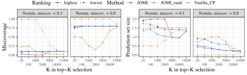
Figure 3: Empirical selection-conditional miscoverage (left) and prediction set size (right) in drug property prediction for vanilla conformal prediction (Vanilla_CP), JOMI and randomized JOMI (JOMI_rand) for test units whose $\widehat{\mu}(X_{n+j})$ are top-$K$ (highest, solid line) or bottom-$K$ (lowest, dashed line) among test units. The reds dashed line is the nominal miscoverage level $\alpha\in\{0.1,0.8\}$. The results are averaged over $N=1000$ runs.

The orange curves (Vanilla_CP) show that vanilla conformal prediction with APS scores is over-confident for units with the lowest predicted affinities while under-confident for units with highest predicted affinities. In contrast, the purple (JOMI) and blue (JOMI_rand) curves both show valid coverage for our proposed methods. Also, using the APS score introduces visible gap between the actual coverage and $1-\alpha$ for JOMI due to discretization, which is made exact by its randomized version.

Interestingly, vanilla conformal prediction with the APS score yields zero-cardinality prediction sets for units with the lowest predicted affinities with $\alpha=0.8$ (the orange dashed line in the right panel of Figure 3). This is because vanilla CP covers other test units with very high rate, and thus marginal coverage is guaranteed even with empty prediction sets for the selected units. Of course, this is worrying if one cares more about these units at the bottom.

The behavior of these methods also depends on the choice of the nonconformity score $V$. Appendix A.2 shows the results for selection rules (i)-(iii) with the binary score $V(x,y)=y(1-\widehat{\mu}(x))+(1-y)\widehat{\mu}(x)$. With the binary score, JOMI consistently achieves valid coverage for selected units, and the coverage gap of JOMI due to discretization is less visible. For vanilla CP, opposite to the situations here, it is over-confident for units with the highest predicted affinities yet under-confident for units with the lowest predicted affinities.

5.1.2 Conformalized selection

We then consider conformalized selection, where the focal test units are those believed to obey $Y=1$ with false discovery rate control at level $q\in(0,1)$. This problem was investigated in Bao et al., (2024) with no exact finite-sample coverage guarantees in theory (though their heuristic method performs reasonably in their empirical studies). We apply conformalized selection (Jin and Candès, 2023b, ) at FDR level $q\in\{0.2,\dots,0.9\}$ and $c_{i}\equiv 0.5$ to determine $\widehat{\mathcal{S}}$, and construct prediction intervals for units in $\widehat{\mathcal{S}}$ using both the APS score and the binary score. Experiments are repeated for $N=1000$ independent runs.

Figure 4 depicts the miscoverage $\widehat{\textnormal{Miscov}}$ and prediction interval lengths with nominal miscoverage level $\alpha\in\{0.1,0.8\}$ under various FDR levels $q$ and two choices of nonconformity score $V$.

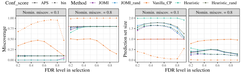
Figure 4: Empirical selection-conditional miscoverage (left) and prediction set size (right) in drug property prediction for test units selected by conformalized selection (for finding $Y=1$ at target FDR levels $q\in\{0.2,\dots,0.9\}$) when applying vanilla conformal prediction (Vanilla_CP), JOMI (JOMI), randomized JOMI (JOMI_rand), the method of Bao et al., (2024) (Heuristic and Heuristic_rand). Results with the APS score are in solid lines, while those with the binary score are in dashed lines. Details are otherwise the same as Figure 3.

Vanilla CP is not calibrated for selected units: it is over-confident with both scores for $\alpha=0.1$, while being over-confident with binary score and under-confident with APS score at $\alpha=0.8$. In contrast, JOMI and JOMI_rand achieves valid selection-conditional coverage in all scenarios. There is some gap for JOMI with the APS score due to discretization, but not for JOMI_rand or the binary score. We observe an even lower empirical FCR than the conditional miscoverage for our methods (so they achieve valid FCR control); this is because the selection set can sometimes be empty for small values of FDR level $q$ (recall Proposition 3). Finally, compared with the heuristic methods of Bao et al., (2024), our method usually achieves smaller prediction set sizes whereas their method seems overly conservative. We conjecture that this is due to a more delicate choice of the reference set.

5.1.3 Selection with constraints

We now consider selecting units with the highest predicted binding affinities within a total budget of subsequent development. In this case, ${\mathcal{S}}({\mathcal{D}}_{\textnormal{calib}},{\mathcal{D}}_{\textnormal{test}})=\{j\in[m]\colon\widehat{\mu}(X_{n+j})\geq\bar{\mu}\}$, where $\bar{\mu}=\max\{\mu\colon\sum_{j=1}^{m}L_{n+j}\mathds{1}\{\widehat{\mu}(X_{n+j})\geq\mu\}\leq C\}$, and $\{L_{n+j}\}_{j\in[m]}$ are the costs.

We create semi-synthetic datasets since the original HIV data does not contain the cost information. Specifically, for each $i\in[n+m]$, we generate $L_{i}=\exp(3\widehat{\mu}(X_{i}))+2|\sin(\widehat{\mu}(X_{i}))|+\epsilon_{i}$, where $\widehat{\mu}(X_{i})$ is the predicted binding affinity, and $\epsilon_{i}\sim\text{Exp}(1)$ are i.i.d. random variables that capture other cost-related information. Setting $20\%$ od the data aside as the training set, we randomly sample the data without replacement so that $n=2500$ and $m=2500$.

The average miscoverage, prediction set size, and reference set size are reported in Figure 5. Interestingly, after adding cost constraints, vanilla conformal prediction is over-confident with the binary score and under-confident with the APS score. In contrast, our methods always yield near-exact coverage. From the right-most plot, we see that $|\widehat{\mathcal{R}}_{j}|$ is positively correlated with the number of selected test units.

Figure 5: Empirical miscoverage rate (left), average length of prediction interval (middle), and scatter plots for averaged reference set size $\{|\widehat{\mathcal{R}}_{j}|\}_{j\in\widehat{{\mathcal{S}}}}$ versus $|\widehat{{\mathcal{S}}}|$ (right), across $N=500$ independent runs of Vanilla_CP, JOMI, and JOMI_rand. The $x$-axis of left and middle plots is the nominal miscoverage level $\alpha\in\{0.1,0.2,\dots,0.9\}$.

5.2 Drug-target-interaction prediction

We now turn to a regression task, drug-target-interaction prediction. We use the DAVIS dataset in the DeepPurpose library (Huang et al.,, 2020). The outcome $Y$ is a continuously-valued variable indicating the binding affinity of a drug-target pair. The features $X$ combine the encodings of the drug compound and the target, where we encode the drug via a convolutional neural network (CNN) structure, and the target via a Transformer encoder. Our framework is agnostic to the choice of these encoding methods.

We train a point predictor $\widehat{\mu}(\cdot)\colon{\mathcal{X}}\to\mathbb{R}$ with $20\%$ randomly selected data in the entire dataset using a small neural network. The remaining $80\%$ data are then randomly split into two equally-sized folds as ${\mathcal{D}}_{\textnormal{calib}}$ and ${\mathcal{D}}_{\textnormal{test}}$. Similar to DPP, the training phase is repeated for $10$ independent runs; within each run, we independently run $100$ random split of calibration/test data and subsequent selection and construction of prediction sets. We use the nonconformity score $V(x,y)=|y-\widehat{\mu}(x)|$ throughout.

5.2.1 Conformalized selection for heterogeneous $c_{n+j}$’s

We then study the behavior of vanilla CP and our proposed methods for selected units by running conformalized selection (Jin and Candès, 2023b, ) to find test pairs $j\in[m]$ whose outcomes are greater than data-dependent thresholds $c_{n+j}$. Here, we set $c_{n+j}$ as the $0.7$-th quantile of activities for training pairs with the same target sequence as the $j$-th data, while controlling the FDR below $q\in\{0.2,0.3,\dots,0.9\}$. The method of Bao et al., (2024) is not applicable to the heterogeneous thresholds here.

Figure 6 shows the miscoverage (the left panel) and average length of prediction intervals (the right panel) using JOMI and vanilla conformal prediction. For those most promising units picked by conformalized selection, vanilla CP (orange) tends to be over-confident with exceedingly high miscoverage. In contrast, our proposed methods achieve near-exact coverage across all values of $q$ and $\alpha$. Again, we observe that the FCR of our methods is even lower than $\widehat{\textnormal{Miscov}}$, empirically yielding valid FCR control.

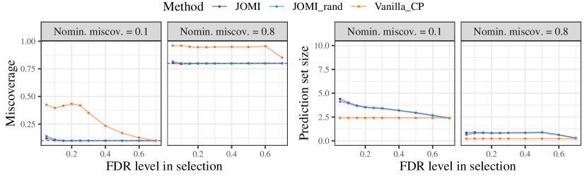
Figure 6: Empirical selection-conditional miscoverage (left) and prediction set size (right) in drug-target-interaction for vanilla conformal prediction (Vanilla_CP) and JOMI (JOMI and JOMI_rand), at nominal miscoverage $\alpha\in\{0.1,0.8\}$ for test units selected by conformalized selection at nominal FDR levels $q\in\{0.2,\dots,0.9\}$.

Our method can sometimes lead to two separate prediction intervals. We calculate the average number of intervals among selected test units in each experiment and report their boxplot in Figure 7. The frequency of producing two segments is very low across all cases.

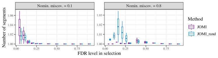
Figure 7: Boxplot of the average number of intervals produced by JOMI and JOMI_rand among selected test units, over $N=1000$ independent runs, at nominal miscoverage $\alpha\in\{0.1,0.8\}$ for various experiment configurations.

5.2.2 Selection under budget constraint

Finally, we consider a covariate-dependent selection rule, where the scientist aims to maximize the predicted activities of selected drugs subject to a fixed budget for subsequent development.

Formally, for each drug-target pair $i\in[m+n]$, we let $c_{i}$ be the $0.7$-th quantile of true activity scores in the training set with the same target, $\widehat{\mu}(X_{i})$ be its predicted binding affinity, and $L_{i}>0$ be its development costs. Then, ${\mathcal{S}}({\mathcal{D}}_{\textnormal{calib}},{\mathcal{D}}_{\textnormal{test}})$ aims to solve the following optimization problem:

$$\mathop{\text{maximize}}_{S\subseteq[m]} \quad\sum_{j\in S}\big{[}\widehat{\mu}(X_{n+j})-c_{n+j}\big{]}$$ (28)

subject to $$\quad\sum_{j\in S}L_{n+j}\leq\bar{L},$$

where $\bar{L}=200$ is a budget limit. Again, as the dataset does not come with drug development costs, we generate $L_{i}=\exp(3\widehat{\mu}(X_{i})/\bar{\mu})+|\sin(\widehat{\mu}(X_{i}))|+\epsilon_{i}-1+\varepsilon_{i}$, where $\bar{\mu}=\max_{i\in{\mathcal{D}}_{\textnormal{train}}}|\widehat{\mu}(X_{i})|$, and $\epsilon_{i}\sim\text{Exp}(1)$, $\varepsilon_{i}\sim\text{Unif}([0,1])$ are independent random variables.

The optimization problem (28) is known as the Knapsack problem which is NP-hard. Nevertheless, there are efficient approximate solvers; in our experiments, we use the Python package mknapsack (mknapsack,, 2023). Existing methods such as Bao et al., (2024) cannot deal with such a complicated selection process. In contrast, our framework tackles this problem with a computation complexity that is polynomial in $m$, $n$, and the complexity of the subroutine ${\mathcal{S}}(\cdot,\cdot)$.

In Figure 8, we report the empirical miscoverage rate, average length of prediction intervals, and the sizes of ${\mathcal{S}}({\mathcal{D}}_{\textnormal{calib}},{\mathcal{D}}_{\textnormal{test}})$ and the reference set $\widehat{\mathcal{R}}_{j}$ for all selected units, across $N=1000$ independent runs of our procedures. While vanilla conformal prediction is over-confident (with a much higher miscoverage rate), our methods yield exact coverage for the focal units. From the length of prediction sets, we see that longer prediction intervals are needed to cover promising drug-target pairs. While the number of selected test units are relatively stable, the reference set size may vary a bit.

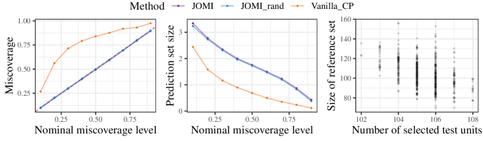
Figure 8: Empirical miscoverage rate (left), average length of prediction interval (middle), and scatter plots for $|{\mathcal{S}}({\mathcal{D}}_{\textnormal{calib}},{\mathcal{D}}_{\textnormal{test}})|$ versus $\{|\widehat{\mathcal{R}}_{j}|\}_{j\in{\mathcal{S}}({\mathcal{D}}_{\textnormal{calib}},{\mathcal{D}}_{\textnormal{test}})}$ (right), across $N=1000$ independent runs of Vanilla_CP, JOMI, and JOMI_rand. The $x$-axis of left and middle plots is the nominal miscoverage level $\alpha\in\{0.1,0.2,\dots,0.9\}$.

6 Application to health risk prediction

Prediction machines are also widely used in healthcare for guiding clinical decision-making. These decisions may come from complicated underlying processes such as clinical resource optimization (Ahmadi-Javid et al.,, 2017; Master et al.,, 2017) or preliminary uncertainty quantification (Olsson et al.,, 2022). Accounting for selections from complicated decision processes is necessary for reliable and informative uncertainty quantification. In this section, we demonstrate the application of our framework to health risk prediction settings where units are picked by complicated processes. We will consider three selection rules:

1. Selection with constraints. Clinical decision makers may optimize a performance measure subject to certain constraints such as budget, capacity, or fairness (Castro and Petrovic,, 2012; Kemper et al.,, 2014; Gocgun and Puterman,, 2014), and send patients to different care categories. In Section 6.1, we consider a stylized example where we minimize the total predicted ICU stay subject to total cost budget, where the selected units can be viewed as patients sent to a certain category.

2. Selecting small conformal prediction sets. Based on preliminary conformal prediction, one may suggest human intervention for units with large set sizes (Olsson et al.,, 2022; Sokol et al.,, 2024) while leaving those with small prediction sets unattended. In Section 6.2, we re-calibrate predictive inference for those whose preliminary prediction sets are shorter than a threshold.

3. Selection based on lower prediction bounds. Practitioners may also focus on units whose preliminary prediction intervals lie above a threshold (Levitskaya,, 2023). In Section 6.3, we study selected test units whose preliminary prediction intervals have lower bounds above a threshold.

Among the above, rule (1) is covariate-dependent, while rules (2) and (3) can depend on the outcomes. All of them are efficiently tackled by the computation tricks in Section 4.

Our experiments use the ICU-stay data in the MIMIC-IV dataset (Johnson et al.,, 2023). Data (and features in $X$) are pre-processed using the pipeline provided by Gupta et al., (2022), with the outcome $Y$ being the length of ICU stay. We use random forests in the scikit-learn Python package to train a point prediction model $\widehat{\mu}(\cdot)$ and two quantile regression models $\widehat{q}_{1-\beta/2}(\cdot)$ and $\widehat{q}_{\beta/2}(\cdot)$ using a holdout training set. Calibration and test data are randomly split with $n=3000$ and $m=2000$.

6.1 Selection with constraints

We first study the case where test units are selected by minimizing the total predicted ICU stay time subject to a budget constraint. Given the point predictor $\widehat{\mu}(\cdot)$, we solve a Knapsack problem similar to (28) using the same approximate algorithm, where we maximize the summation of $\widehat{\mu}(X_{n+j})$ in the selected subset, and the cost $L_{n+j}$ is generated in the same way as Section 5.2.2 and then taken the ceiling.

Figure 9 shows the empirical miscoverage rate, length of prediction interval, and sizes of the selection set and reference sets. While vanilla conformal prediction is over-confident, our method achieves exact coverage for selected test units. We also see a slightly positive correlation of $|\widehat{\mathcal{R}}_{n+j}|$ and $|\widehat{{\mathcal{S}}}|$.

Figure 9: Empirical miscoverage rate (left), average length of prediction interval (middle), and scatter plots for the averaged reference set size versus $|\widehat{{\mathcal{S}}}|$ (right), across $N=500$ independent runs of Vanilla_CP, JOMI, and JOMI_rand. The $x$-axis of left and middle plots is the nominal miscoverage level $\alpha\in\{0.1,0.2,\dots,0.9\}$.

6.2 Selecting small-sized prediction sets

We then consider the second selection rule, where we first build preliminary conformal prediction intervals $\widehat{C}_{\alpha,n+j}^{\text{prelim}}$ via the score function $S(x,y)=|y-\widehat{\mu}(x)|/\widehat{\sigma}(x)$ (Lei et al.,, 2018); both the point prediction function $\widehat{\mu}(\cdot)$ and the conditional standard deviation are estimated via random forests. We then select those test units with $|\widehat{C}_{\alpha,n+j}^{\text{prelim}}|\leq 5$, i.e., the upper and lower bounds of the preliminary prediction intervals are less than $5$ days apart. This mimics the ideas in (Ren et al.,, 2023; Sokol et al.,, 2024) where small-sized prediction sets are “certified” as confident.

After selection, we leverage the method in Section 4.3 to construct $\widehat{C}^{\textrm{ps}}_{\alpha,n+j}$ for all selected test units. Since $\widehat{C}^{\textrm{ps}}_{\alpha,n+j}$ is a superset of the exact output $\widehat{C}_{\alpha,n+j}$, we evaluate its empirical coverage to investigate whether it is over-conservative. Also, note from (26) that it is the union of three subsets; we also evaluate the number of disjoint segments in $\widehat{C}^{\textrm{ps}}_{\alpha,n+j}$.

The miscoverage and length of prediction sets are reported in the left and middle plots in Figure 10. We observe that selectively certifying short prediction intervals can lead to under-coverage (orange curve), while JOMI achieves exact coverage (purple curve) by inflating the prediction sets, meaning that the superset $\widehat{C}^{\textrm{ps}}_{\alpha,n+j}$ is effectively quite tight. The average number of disjoint segments in the right plot of Figure 10, which shows that $\widehat{C}^{\textrm{ps}}_{\alpha,n+j}$ is almost always one single interval.

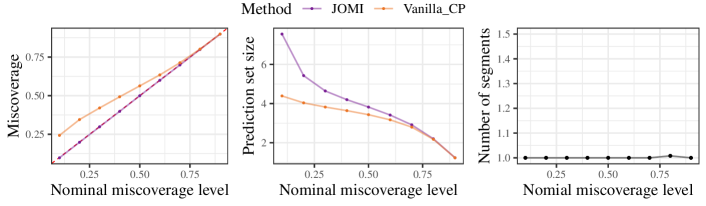
Figure 10: Empirical miscoverage rate (left), average length of prediction interval (middle), and average number of segments in $\widehat{C}^{\textrm{ps}}_{\alpha,n+j}$ (right), across $N=500$ independent runs of Vanilla_CP and JOMI when test units with short preliminary prediction sets are selected. The $x$-axis are nominal miscoverage levels $\alpha\in\{0.1,0.2,\dots,0.9\}$.

6.3 Selecting prediction sets below a threshold

Finally, we study selection rule (iii) which is also based on a preliminary prediction set constructed in the same away as Section 6.2. We imagine that practitioners select a test unit $n+j$ if the upper bound of $\widehat{C}^{\text{pre}}_{\alpha,n+j}$ is below $6$, i.e., it appears the patient will stay in ICU less than 6 days.

The miscoverage rate, length of prediction sets, and number of disjoint segments averaged over $N=500$ independent runs of JOMI (using the method in Section 4.3) and vanilla conformal prediction are summarized in Figure 11. We see that preliminary prediction sets with low upper bounds tend to under-cover for small $\alpha$, while JOMI achieves exact coverage despite that we construct a superset of $\widehat{C}_{\alpha,n+j}$. However, JOMI may produce multiple segments for large values of $\alpha$.

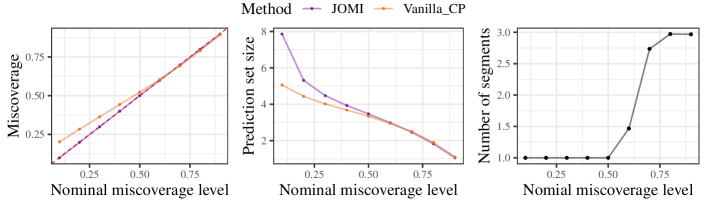
Figure 11: Empirical miscoverage rate (left), average length of prediction interval (middle), and average number of segments in $\widehat{C}^{\textrm{ps}}_{\alpha,n+j}$ (right), across $N=500$ independent runs of Vanilla_CP and JOMI. The nominal miscoverage levels on the $x$-axis are $\alpha\in\{0.1,0.2,\dots,0.9\}$.

Reproducibility

The code for reproducing the experimental results in this paper is available at https://github.com/ying531/JOMI-paper.

Appendix A Additional experiment results

This section collects additional experimental results that are omitted in the main text. Appendix A.1 shows results for DPP with selection rules (ii) and (iii) with the APS score, omitted in Section 5.1. Appendix A.2 shows results for DPP with selection rules (i)-(iii) with the binary score. Appendix A.3 shows results for DTI with selection rules (ii) and (iii) that are omitted in Section 5.2.

A.1 Additional results for APS score in drug property prediction

In this part, we present results for DPP when test units are selected via (ii) top-K in both calibration and test data (Appendix A.1.1), and (iii) only calibration data as reference (Appendix A.1.2).

A.1.1 Top-K selection in mixed sample

We use the same values of $(\alpha,K)$ and the same scheme of repeated experiments as in Section 5.1.1, with $\mathfrak{S}=2^{[m]}$. Figure 12 shows that vanilla conformal prediction incurs a large coverage gap for selected units, while JOMI and its randomized version both achieve valid selection-conditional coverage. The coverage gap due to discretization is eliminated again by randomization. Randomization also reduces the prediction set sizes on the right panel, but again, with $\alpha=0.8$, we see the concerning issue that it suffices for vanilla CP to construct empty prediction sets for selected units to achieve marginal coverage.

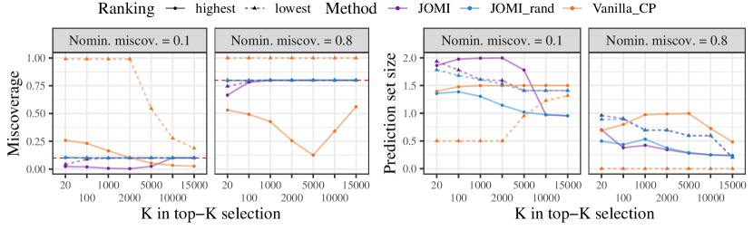
Figure 12: Empirical selection-conditional miscoverage (left) and prediction set size (right) in drug property prediction for test units whose $\widehat{\mu}(X_{n+j})$ are top-K (highest, solid line) or bottom-K (lowest, dashed line) among both calibration and test units. Details are otherwise the same as Figure 3.

A.1.2 Calibration-referenced selection

Now we select test units whose predicted affinities must be greater (or smaller) than the $K$-th largest (or smallest) predictions in the calibration set. We use the choices of $(\alpha,K)$ and the scheme of repeated experiments as in Section 5.1.1 with $\mathfrak{S}=2^{[m]}$.

Figure 13: Empirical selection-conditional miscoverage (left) and prediction set size (right) in drug property prediction for test units selected by (iii) whose $\widehat{\mu}(X_{n+j})$ are greater than the $K$-th highest (solid line) or smaller than the $K$-th lowest (dashed line) in calibration units. Details are otherwise as Figure 3.

Figure 13 shows that our proposed methods achieve valid coverage (exact with JOMI_rand) while vanilla conformal prediction fails to. Again, vanilla CP is either over-confident or under-confident for units with lowest or highest predicted affinities.

A.2 Additional results for binary score in drug property prediction

In Figures 14, 15, and 16, we show the empirical selection-conditional coverage and prediction set sizes for selection rules (i)-(iii) when the prediction sets are constructed with the binary score $V(x,y)=y(1-\widehat{\mu}(x))+(1-y)\widehat{\mu}(x)$. We observe that while vanilla CP is either over-confident or under-confident, our proposed methods achieve valid coverage across all configurations. The coverage gap of the non-randomized JOMI is smaller with this specific score function compared with the APS score.

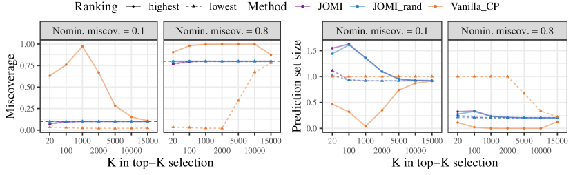
Figure 14: Empirical selection-conditional miscoverage (left) and prediction set size (right) in drug property prediction with the binary score, for test units selected by (i) top-K (or bottom-K) in test data. Details are otherwise as Figure 3.

Figure 15: Empirical selection-conditional miscoverage (left) and prediction set size (right) in drug property prediction with the binary score, for test units selected by (ii) top-K (or bottom-K) in both calibration and test data. Details are otherwise as Figure 12.

Figure 16: Empirical selection-conditional miscoverage (left) and prediction set size (right) in drug property prediction with the binary score, for test units that are (iii) greater than the $K$-th highest (or smaller than the $K$-th lowest) predicted affinities in the calibration data. Details are as Figure 13.

A.3 Additional results for drug-target-interaction prediction

In this section, we collect results for DTI with (1) covariate dependent top-K selection. We present results under selection rule (1-i) in Appendix A.3.1, (1-ii) in Appendix A.3.2 and (1-iii) in Appendix A.3.3.

A.3.1 Top-K selection for fixed K

We consider the case where test units are selected via (i) top-K (or bottom-K) among predicted affinities in the test set. We apply the vanilla conformal prediction and our proposed methods with $\mathfrak{S}=2^{[m]}$, so that selection-conditional coverage implies FCR control. Results under selection rules (ii) and (iii) demonstrate similar patterns, which we defer to Appendix A.3.

Figure 17 shows $\widehat{\textrm{Miscov}}$ (the left panel) and the average length of the prediction intervals (the right panel) for $K\in\{20,100,1000,2000,5000,10000\}$ and nominal miscoverage level $\alpha\in\{0.1,0.8\}$. We see that vanilla conformal prediction is over-confident for pairs with the highest predicted affinities, while being under-confident for the lowest. In contrast, our proposed methods achieve near-exact coverage under different nominal levels. By comparing the solid and dashed lines in the right panel, we observe that in this problem, the intrinsic uncertainty in higher-predicted-affinity pairs is larger, so a longer prediction interval is needed to achieve certain coverage.

Figure 17: Empirical miscoverage (left) and prediction interval length (right) in drug-target-interaction prediction, for vanilla conformal prediction (Vanilla_CP), JOMI (JOMI), and randomized JOMI applied to test units whose $\widehat{\mu}(X_{n+j})$ are top-$K$ (highest, solid line) or bottom-$K$ (lowest, dashed line) among test units. The red dashed line is the nominal miscoverage level $\alpha\in\{0.1,0.8\}$.

A.3.2 Top-K selection in mixed sample

Figure 18 shows the miscoverage and average length of prediction intervals when (ii) the focal test units are those whose predicted affinities are among the $K$ highest or lowest in both calibration and test data. We see that vanilla CP is over-confident for highest-prediction units, while under-confident for lowest-prediction units. In contrast, our proposed methods always yield valid coverage.

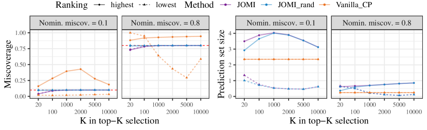
Figure 18: Empirical miscoverage (left) and prediction interval length (right) in drug-target-interaction prediction, for selected test units whose $\widehat{\mu}(X_{n+j})$ are top-$K$ among both calibration and test units. Details are otherwise the same as Figure 3.

A.3.3 Calibration-referenced selection

Figure 19 shows the results with (iii) calibration-referenced selection, i.e., the selected test units are those whose predicted affinities are greater than (or smaller than) the $K$-th highest (or lowest) in the calibration data. Similar to rules (i) and (ii), vanilla CP is not calibrated for these focal units, while our methods yield near-exact coverage across the whole spectrum of $K$.

Figure 19: Empirical FCR in drug-target interaction prediction, for selected test units whose $\widehat{\mu}(X_{n+j})$ surpass the highest $K$ predicted affinities in the calibration data (or smaller than the lowest). Details are otherwise the same as Figure 17.

Appendix B Technical proofs

B.1 Proof of Proposition 1

Suppose $\widehat{C}_{\alpha,n+j}$ satisfies (3) for a set of mutually disjoint taxonomies $\{\mathfrak{S}_{\ell}\}_{\ell\in{\mathcal{L}}}$ such that $\cup_{\ell\in{\mathcal{L}}}\mathfrak{S}_{\ell}=2^{[m]}$. Then

$$\mathbb{P}(Y_{n+j}\in\widehat{C}_{\alpha,n+j}{\,|\,}j\in\widehat{\mathcal{S}}) \stackrel{{\scriptstyle\textrm{(a)}}}{{=}}\sum_{\ell\in{\mathcal{L}}}\mathbb{P}\big{(}Y_{n+j}\in\widehat{C}_{\alpha,n+j},\widehat{{\mathcal{S}}}\in\mathfrak{S}_{\ell}\,\big{|}\,j\in\widehat{\mathcal{S}}\big{)}$$

$$=\sum_{\ell\in{\mathcal{L}}}\mathbb{P}\big{(}Y_{n+j}\in\widehat{C}_{\alpha,n+j}\,\big{|}\,j\in\widehat{\mathcal{S}},\widehat{\mathcal{S}}\in\mathfrak{S}_{\ell}\big{)}\cdot\mathbb{P}(\widehat{\mathcal{S}}\in\mathfrak{S}_{\ell}{\,|\,}j\in\widehat{{\mathcal{S}}})$$

$$\stackrel{{\scriptstyle\textrm{(b)}}}{{\geq}}(1-\alpha)\cdot\sum_{\ell\in{\mathcal{L}}}\mathbb{P}(\widehat{\mathcal{S}}\in\mathfrak{S}_{\ell}{\,|\,}j\in\widehat{{\mathcal{S}}})=1-\alpha,$$

where in the first step we use the fact that $\{\mathfrak{S}_{\ell}\}_{\ell\in{\mathcal{L}}}$ are disjoint and their union is the full set, and the second step follows from the strong selection-conditional coverage. By definition, it satisfies the weak selection-conditional coverage (2).

B.2 Proof of Proposition 2

Suppose $\widehat{C}_{\alpha,n+j}$ satisfies the strong selection-conditional coverage (3) for a class of mutually disjoint taxonomies $\{\mathfrak{S}_{\ell}\}_{\ell\in{\mathcal{L}}}$ such that $\cup_{\ell\in{\mathcal{L}}}\mathfrak{S}_{\ell}=2^{[m]}$, and for each $\ell\in{\mathcal{L}}$, it holds that $\mathfrak{S}_{\ell}\subseteq\{S\subseteq[m]\colon|S|=r(\ell)\}$ for some $0\leq r(\ell)\leq m$. By definition, and since $\{\mathfrak{S}_{\ell}\}_{\ell\in{\mathcal{L}}}$ are disjoint, we have

FCR $$=\mathbb{E}\bigg{[}\frac{\sum_{j\in[m]}\mathds{1}\{j\in\widehat{{\mathcal{S}}},Y_{n+j}\notin\widehat{C}_{\alpha,n+j}\}}{|\widehat{{\mathcal{S}}}|\vee 1}\bigg{]}$$ (29)

$$=\sum_{\ell\in{\mathcal{L}}}\mathbb{E}\bigg{[}\mathds{1}\{\widehat{{\mathcal{S}}}\in\mathfrak{S}_{\ell}\}\cdot\frac{\sum_{j\in[m]}\mathds{1}\{j\in\widehat{{\mathcal{S}}},Y_{n+j}\notin\widehat{C}_{\alpha,n+j}\}}{|\widehat{{\mathcal{S}}}|\vee 1}\bigg{]}.$$ (30)

Noting that $\mathfrak{S}_{\ell}\subseteq\{S\subseteq[m]\colon|S|=r(\ell)\}$ hence $|\widehat{{\mathcal{S}}}|=r(\ell)$ when $\widehat{{\mathcal{S}}}\in\mathfrak{S}_{\ell}$, we can rewrite the above as

$$\sum_{\ell\in{\mathcal{L}}}\sum^{m}_{j=1}\frac{1}{r(\ell)\vee 1}\mathbb{E}\big{[}\mathds{1}\big{\{}\widehat{{\mathcal{S}}}\in\mathfrak{S}_{\ell},j\in\widehat{{\mathcal{S}}},Y_{n+j}\notin\widehat{C}_{\alpha,n+j}\big{\}}\big{]}$$

$$=\leavevmode\nobreak\ \sum_{\ell\in{\mathcal{L}}}\sum^{m}_{j=1}\frac{1}{r(\ell)\vee 1}\mathbb{E}\Big{[}\mathds{1}\{\widehat{{\mathcal{S}}}\in\mathfrak{S}_{\ell},j\in\widehat{{\mathcal{S}}}\}\cdot\mathbb{E}\big{[}\mathds{1}\{Y_{n+j}\notin\widehat{C}_{\alpha,n+j}\}\,\big{|}\,\mathds{1}\{j\in\widehat{{\mathcal{S}}},\widehat{{\mathcal{S}}}\in\mathfrak{S}_{\ell}\}\big{]}\Big{]}$$

$$=\leavevmode\nobreak\ \sum_{\ell\in{\mathcal{L}}}\sum^{m}_{j=1}\frac{1}{r(\ell)\vee 1}\mathbb{E}\Big{[}\mathds{1}\{\widehat{{\mathcal{S}}}\in\mathfrak{S}_{\ell},j\in\widehat{{\mathcal{S}}}\}\cdot\mathbb{P}\big{(}Y_{n+j}\notin\widehat{C}_{\alpha,n+j}\,\big{|}\,j\in\widehat{{\mathcal{S}}},\widehat{{\mathcal{S}}}\in\mathfrak{S}_{\ell}\big{)}\Big{]}$$

$$\leq\leavevmode\nobreak\ \sum_{\ell\in{\mathcal{L}}}\sum^{m}_{j=1}\frac{\alpha}{r(\ell)\vee 1}\mathbb{E}\big{[}\mathds{1}\{j\in\widehat{{\mathcal{S}}},\widehat{{\mathcal{S}}}\in\mathfrak{S}_{\ell}\}\big{]},$$ (31)

where the last inequality follows from the strong selection-conditional coverage. Finally, the FCR control proof is completed by noting that

$$\eqref{eq:fcr_step2}=\sum_{\ell\in{\mathcal{L}}}\frac{\alpha}{r(\ell)\vee 1}\mathbb{E}\Big{[}|\widehat{{\mathcal{S}}}|\cdot\mathds{1}\{\widehat{{\mathcal{S}}}\in\mathfrak{S}_{\ell}\}\Big{]}=\alpha\cdot\mathbb{P}\big{(}\widehat{{\mathcal{S}}}\neq\varnothing\big{)}\leq\alpha.$$

B.3 Proof of Proposition 3

Consider the following example with $m=2$ test units and ${\mathcal{Y}}=\mathbb{R}$. Suppose the target miscoverage level $\alpha\in(0,1)$, and the selection rule returns

$$\widehat{{\mathcal{S}}}=\begin{cases}\{1,2\}&\text{with probability }1-\frac{2\alpha}{1+\alpha},\\ \{1\}&\text{with probability }\frac{\alpha}{1+\alpha},\\ \{2\}&\text{with probability }\frac{\alpha}{1+\alpha}.\end{cases}$$

Consider prediction sets $\widehat{C}_{\alpha,n+1}$ and $\widehat{C}_{\alpha,n+2}$ such that

• when $\widehat{{\mathcal{S}}}=\{1,2\}$, $\widehat{C}_{\alpha,n+1}=\mathbb{R},\widehat{C}_{\alpha,n+2}=\mathbb{R}$;

• when $\widehat{{\mathcal{S}}}=\{1\}$, $\widehat{C}_{\alpha,n+1}=\varnothing$;

• when $\widehat{{\mathcal{S}}}=\{2\}$, $\widehat{C}_{\alpha,n+2}=\varnothing$.

We can check that the weak selection-conditional coverage is satisfied for $j=1$:

$$\mathbb{P}(Y_{n+1}\in\widehat{C}_{\alpha,n+1}{\,|\,}1\in\widehat{{\mathcal{S}}})=\frac{\mathbb{P}(Y_{n+1}\in\widehat{C}_{\alpha,n+1},1\in\widehat{{\mathcal{S}}})}{\mathbb{P}(1\in\widehat{{\mathcal{S}}})}=\frac{1-2\alpha/(1+\alpha)}{1-2\alpha/(1+\alpha)+\alpha/(1+\alpha)}=1-\alpha.$$

By symmetry, the weak selection-conditional coverage is also satisfied for $j=2$. Meanwhile, one can check that

$$\text{FCR}=\frac{\alpha}{1+\alpha}+\frac{\alpha}{1+\alpha}=\frac{2\alpha}{1+\alpha}>\alpha.$$

Therefore, the constructed prediction sets $\widehat{C}_{\alpha,n+1}$ and $\widehat{C}_{\alpha,n+2}$ satisfy the weak selection-conditional coverage but violate the FCR control.

B.4 Proof of Theorem 1

Recall that ${\mathcal{D}}_{j}={\mathcal{D}}_{{\textnormal{calib}}}\cup\{Z_{n+j}\}$ and ${\mathcal{D}}_{j}^{c}=\{X_{n+\ell}\}_{\ell\in[m]\backslash\{j\}}$. For notational convenience, we also denote the index sets ${\mathcal{I}}_{j}=[n]\cup\{n+j\}$ and ${\mathcal{I}}_{j}^{c}=[m]\backslash\{j\}$. Let $[{\mathcal{D}}_{j}]=[Z_{1},\dots,Z_{n},Z_{n+j}]$ be the unordered set of ${\mathcal{D}}_{j}$, and we denote the realized value of the unordered set as $[d_{j}]=[z_{1},\dots,z_{n},z_{n+j}]$, i.e., $z_{i}$’s are fixed realized values of $Z_{i}$’s, but we do not know which values in $[d_{j}]$ correspond to the calibration set and which to the test point. We also write $z_{i}=(x_{i},y_{i})$ and $v_{i}=V(x_{i},y_{i})$, with $x_{i}$ and $y_{i}$ being the realized values of $X_{i}$ and $Y_{i}$. We then prove the two statements separately.

Proof of (a).

To prove (12), it suffices to show that

$$\mathbb{P}\Big{(}V_{n+j}\leq{\textnormal{Quantile}}\big{(}1-\alpha;\{V_{i}\}_{i\in\widehat{{\mathcal{R}}}_{n+j}(Y_{n+j})}\cup\{+\infty\}\big{)}\,\Big{|}\,j\in\widehat{\mathcal{S}},\,\widehat{{\mathcal{S}}}\in\mathfrak{S}\Big{)}\geq 1-\alpha.$$ (32)

The exchangeability of data in ${\mathcal{D}}_{j}$ given ${\mathcal{D}}_{j}^{c}$ implies that, given knowledge of the unordered realized data values in $[d_{j}]$, the probability of any assignment of these values to the data points is equal. That is, for any permutation $\pi$ of ${\mathcal{I}}_{j}$,

$$\mathbb{P}\big{(}Z_{1}=z_{\pi(1)},\dots,Z_{n}=z_{\pi(n)},Z_{n+j}=z_{\pi(n+j)}\,\big{|}\,[d_{j}],{\mathcal{D}}_{j}^{c}\big{)}=\frac{1}{(n+1)!}.$$

Next, given $[d_{j}]$ and ${\mathcal{D}}_{j}^{c}$, we define the following subset of ${\mathcal{I}}_{j}$:

$$\widetilde{R}=\big{\{}i\in{\mathcal{I}}_{j}\colon j\in{\mathcal{S}}([D_{\textnormal{calib}}^{i}],D_{\textnormal{test}}^{i}),\,{\mathcal{S}}([D_{\textnormal{calib}}^{i}],D_{\textnormal{test}}^{i})\in\mathfrak{S}\big{\}},$$

where $[D_{\textnormal{calib}}^{i}]=[z_{1},\dots,z_{i-1},z_{n+j},z_{i+1},\dots,z_{n}]$ is an unordered set ($[d_{j}]$ with $z_{i}$ removed) and $D_{\textnormal{test}}^{i}=(X_{n+1},\dots,x_{i},\dots,X_{n+m})$. Note that the collection $\{{\mathcal{S}}([D_{\textnormal{calib}}^{i}],D_{\textnormal{test}}^{i})\}_{i\in{\mathcal{I}}_{j}}$ is fully determined by $[d_{j}]$ and ${\mathcal{D}}_{j}^{c}$, so $\widetilde{R}$ is also fully determined by $[d_{j}]$ and ${\mathcal{D}}_{j}^{c}$.

Recall that $\widehat{\mathcal{R}}_{n+j}(Y_{n+j})=\{i\in[n]:j\in\widehat{{\mathcal{S}}}^{{\textnormal{swap}(i,j)}},\,\widehat{{\mathcal{S}}}^{{\textnormal{swap}(i,j)}}\in\mathfrak{S}\}$. We let $\widehat{\mathcal{R}}^{+}_{n+j}=\widehat{\mathcal{R}}_{n+j}(Y_{n+j})$ if $j\notin\widehat{\mathcal{S}}$ and $\widehat{{\mathcal{S}}}\in\mathfrak{S}$ and $\widehat{\mathcal{R}}^{+}_{n+j}=\widehat{\mathcal{R}}_{n+j}(Y_{n+j})\cup\{n+j\}$ otherwise. We claim that given $[d_{j}]$ and ${\mathcal{D}}_{j}^{c}$,

$$\{V_{i}\colon i\in\widehat{\mathcal{R}}_{n+j}^{+}\}=\{v_{i}\colon i\in\widetilde{R}\},$$ (33)

where repetition of elements is allowed on both sides. To see this, let $\pi$ denote the permutation on ${\mathcal{I}}_{j}$ such that $V_{i}=v_{\pi(i)}$ and $V_{n+j}=v_{\pi(n+j)}$. Then

$$\widehat{\mathcal{S}}={\mathcal{S}}\big{(}\underbrace{[z_{\pi(1)},z_{\pi(2)},\dots,z_{\pi(n)}]}_{\textrm{calibration data}},\underbrace{X_{n+1},\dots,x_{\pi(n+j)},\dots,X_{n+m}}_{\textrm{test data}}\big{)}={\mathcal{S}}\big{(}[D_{\textnormal{calib}}^{\pi(n+1)}],D_{\textnormal{test}}^{\pi(n+1)}\big{)},$$ (34)

$$\widehat{\mathcal{S}}^{{\textnormal{swap}(i,j)}}={\mathcal{S}}\big{(}\underbrace{[z_{\pi(1)},\dots,z_{\pi(i-1)},z_{\pi(n+j)},z_{\pi(i+1)},\dots,z_{\pi(n)}]}_{\textrm{calibration data after swap}},\underbrace{X_{n+1},\cdots,x_{\pi(i)},\dots,X_{n+m}}_{\textrm{test data after swap}}\big{)}$$

$$\qquad\qquad={\mathcal{S}}\big{(}[D_{\textnormal{calib}}^{\pi(i)}],D_{\textnormal{test}}^{\pi(i)}\big{)}$$

for all $i\in\{1,\dots,n\}$. Denoting $\widehat{\mathcal{S}}=\widehat{\mathcal{S}}^{{\textnormal{swap}(n+j,j)}}$ for notational simplicity, we have,

$$\{V_{i}\colon i\in\widehat{\mathcal{R}}_{n+j}^{+}\} \overset{\rm(a)}{=}\big{\{}V_{i}\colon i\in{\mathcal{I}}_{j},j\in\widehat{\mathcal{S}}^{{\textnormal{swap}(i,j)}},\,\widehat{{\mathcal{S}}}^{{\textnormal{swap}(i,j)}}\in\mathfrak{S}\big{\}}$$

$$\overset{\rm(b)}{=}\big{\{}v_{\pi(i)}\colon i\in{\mathcal{I}}_{j},j\in\widehat{\mathcal{S}}^{{\textnormal{swap}(i,j)}},\,\widehat{{\mathcal{S}}}^{\textnormal{swap}(i,j)}\in\mathfrak{S}\big{\}}$$

$$\overset{\rm(c)}{=}\big{\{}v_{\pi(i)}\colon i\in{\mathcal{I}}_{j},j\in{\mathcal{S}}\big{(}[D_{{\textnormal{calib}}}^{\pi(i)}],D_{{\textnormal{test}}}^{\pi(i)}\big{)},\,{\mathcal{S}}\big{(}[D_{\textnormal{calib}}^{\pi(i)}],D_{\textnormal{test}}^{\pi(i)}\big{)}\in\mathfrak{S}\big{\}}$$

$$=\big{\{}v_{\ell}\colon\ell\in{\mathcal{I}}_{j},j\in{\mathcal{S}}\big{(}[D_{{\textnormal{calib}}}^{\ell}],D_{{\textnormal{test}}}^{\ell}\big{)},\,{\mathcal{S}}\big{(}[D_{\textnormal{calib}}^{\ell}],D_{\textnormal{test}}^{\ell}\big{)}\in\mathfrak{S}\big{\}}$$

$$\overset{\rm(d)}{=}\{v_{i}\colon i\in\widetilde{R}\}.$$

Above, step (a) follows from the definition of $\widehat{\mathcal{R}}_{n+j}^{+}$; steps (b) and (c) are due to (LABEL:eq:representation), and step (d) follows from the definition of ${\widetilde{R}}$. We thus completed the proof of Equation (33).

Returning to the proof of (32), we have that

$$\mathbb{P}\Big{(}V_{n+j}\leq{\textnormal{Quantile}}\big{(}1-\alpha;\{V_{i}\}_{i\in\widehat{{\mathcal{R}}}_{n+j}(Y_{n+j})}\cup\{+\infty\}\big{)}\,\Big{|}\,j\in\widehat{\mathcal{S}},\leavevmode\nobreak\ \widehat{{\mathcal{S}}}\in\mathfrak{S},\leavevmode\nobreak\ [d_{j}],{\mathcal{D}}_{j}^{c}\Big{)}$$ (35)

$$=\leavevmode\nobreak \mathbb{P}\Big{(}V_{n+j}\leq{\textnormal{Quantile}}\big{(}1-\alpha;\{V_{i}\}_{i\in\widehat{{\mathcal{R}}}_{n+j}^{+}(Y_{n+j})}\big{)}\,\Big{|}\,j\in\widehat{\mathcal{S}},\leavevmode\nobreak\ \widehat{{\mathcal{S}}}\in\mathfrak{S},\leavevmode\nobreak\ [d_{j}],{\mathcal{D}}_{j}^{c}\Big{)}$$

$$=\leavevmode\nobreak \frac{\mathbb{P}\big{(}V_{n+j}\leq{\textnormal{Quantile}}\big{(}1-\alpha;\{V_{i}\}_{i\in\widehat{{\mathcal{R}}}_{n+j}^{+}(Y_{n+j})}\big{)},j\in\widehat{\mathcal{S}},\widehat{{\mathcal{S}}}\in\mathfrak{S}\,\big{|}\,[d_{j}],{\mathcal{D}}_{j}^{c}\big{)}}{\mathbb{P}\big{(}j\in\widehat{\mathcal{S}},\widehat{{\mathcal{S}}}\in\mathfrak{S}\,\big{|}\,[d_{j}],{\mathcal{D}}_{j}^{c}\big{)}},$$

where the last step is due to Bayes’ rule. Again, given $[d_{j}]$ and ${\mathcal{D}}_{j}^{c}$, the only randomness is the assignment of $[z_{1},\dots,z_{n},z_{n+j}]$ to $(Z_{1},\dots,Z_{n},Z_{n+j})$. By (33),

$$\mathbb{P}\Big{(}V_{n+j}\leq{\textnormal{Quantile}}\Big{(}1-\alpha;\{V_{i}\}_{i\in{\mathcal{R}}_{n+j}^{+}(Y_{n+j})}\Big{)},j\in\widehat{\mathcal{S}},\widehat{{\mathcal{S}}}\in\mathfrak{S}\,\Big{|}\,[d_{j}],{\mathcal{D}}_{j}^{c}\Big{)}$$

$$=\leavevmode\nobreak\ \mathbb{P}\Big{(}V_{n+j}\leq{\textnormal{Quantile}}\big{(}1-\alpha;\{v_{i}\colon i\in\widetilde{R}\}\big{)},j\in\widehat{\mathcal{S}},\widehat{{\mathcal{S}}}\in\mathfrak{S}\,\Big{|}\,[d_{j}],{\mathcal{D}}_{j}^{c}\Big{)}$$ (36)

$$=\leavevmode\nobreak\ \sum_{\ell\in{\mathcal{I}}_{j}}\mathbb{P}\big{(}V_{n+j}=v_{\ell},v_{\ell}\leq{\textnormal{Quantile}}\big{(}1-\alpha;\{v_{i}\colon i\in\widetilde{R}\}\big{)},\ell\in{\widetilde{R}}\,\big{|}\,[d_{j}],{\mathcal{D}}^{c}_{j}\big{)}.$$ (37)

Since ${\widetilde{R}}$ is deterministic conditional on $[d_{j}]$ and ${\mathcal{D}}_{j}^{c}$, we know that

$$\eqref{eq:prob_numer}=\leavevmode\nobreak\ \sum_{\ell\in{\widetilde{R}}}\mathbb{P}\big{(}V_{n+1}=v_{\ell}\,\big{|}\,[d_{j}],{\mathcal{D}}_{j}^{c}\big{)}\cdot\mathds{1}\{v_{\ell}\leq{\textnormal{Quantile}}\big{(}1-\alpha;\{v_{i}\colon i\in\widetilde{R}\}\}$$ (38)

$$=\leavevmode\nobreak\ \sum_{\ell\in{\widetilde{R}}}\frac{\mathds{1}\{v_{\ell}\leq{\textnormal{Quantile}}\big{(}1-\alpha;\{v_{i}\colon i\in\widetilde{R}\}\}}{n+1},$$ (39)

where the last step is because $\mathbb{P}(Z_{n+1}=z_{\ell}{\,|\,}[D_{n+1}],{\mathcal{D}}_{n+1}^{c})=1/(n+1)$ for every $\ell$. By the definition of the quantile function,

$$\eqref{eq:numer_deter}\geq\frac{(1-\alpha)|\widetilde{R}|}{n+1}.$$

On the other hand, it is straightforward that

$$\mathbb{P}\big{(}j\in\widehat{\mathcal{S}},\widehat{{\mathcal{S}}}\in\mathfrak{S}\,\big{|}\,[d_{j}],{\mathcal{D}}_{j}^{c}\big{)} =\sum_{i\in{\mathcal{I}}_{j}}\mathbb{P}\big{(}Z_{n+j}=z_{i}\,\big{|}\,[d_{j}],{\mathcal{D}}_{j}^{c}\big{)}\cdot\mathds{1}\{i\in{\widetilde{R}}\}$$ (40)

$$=\sum_{i\in{\mathcal{I}}_{j}}\frac{\mathds{1}\{i\in\widetilde{R}\}}{n+1}=\frac{|\widetilde{R}|}{n+1}.$$ (41)

Combining the above and (41), we have thus verified (LABEL:eq:equiv_cond_cov3). Then by the tower property, we conclude (32), and thus (12).

When the elements in ${\widetilde{R}}$ are distinct, we additionally have the following deterministic inequality following from the definition of the quantile function:

$$\eqref{eq:numer_deter}\leq\frac{(1-\alpha)|{\widetilde{R}}|+1}{n+1},$$

which then leads to

$$\mathbb{P}\Big{(}V_{n+j}\leq{\textnormal{Quantile}}\Big{(}1-\alpha;\{V_{i}\}_{i\in{\mathcal{R}}_{n+j}^{+}(Y_{n+j})}\Big{)}\,\Big{|}\,j\in\widehat{\mathcal{S}},\widehat{{\mathcal{S}}}\in\mathfrak{S},[d_{j}],{\mathcal{D}}_{j}^{c}\Big{)}$$

$$\leq\leavevmode\nobreak\ 1-\alpha+\frac{1}{|\widetilde{R}|}=1-\alpha+\frac{1}{|\widehat{{\mathcal{R}}}_{n+j}^{+}(Y_{n+j})|}=1-\alpha+\frac{1}{1+|\widehat{{\mathcal{R}}}_{n+j}(Y_{n+j})|},$$

where the last step is because we are conditioning on the event $j\in\widehat{\mathcal{S}}$. Taking expectation with respect to $[d_{j}]$ and ${\mathcal{D}}_{j}^{c}$ on both sides, we obtain (13) and complete the proof of statement (a).

Proof of (b).

To conveniently denote repeated values in $[z_{1},\dots,z_{n},z_{n+j}]$ and $[v_{1},\dots,v_{n},v_{n+j}]$ we let $[1],[2],\dots,[n],[n+j]$ be a permutation of ${\mathcal{I}}_{j}$ so that $v_{[1]}\leq v_{[2]}\leq\cdots\leq v_{[n]}\leq v_{[n+j]}$. Then $[d_{j}]$ can be equivalently represented by $\{z_{[i]}\}_{i\in{\mathcal{I}}_{j}}$, and for any $i\in{\mathcal{I}}_{j}$,

$$\mathbb{P}\big{(}Z_{n+j}=z_{[i]}\,\big{|}\,[d_{j}],{\mathcal{D}}_{j}^{c}\big{)}=\frac{1}{n+1}.$$

Following the proof of part (a), we know that

$$\mathbb{P}\big{(}j\in\widehat{\mathcal{S}}\,\big{|}\,[d_{j}],{\mathcal{D}}_{j}^{c}\big{)}=\frac{|\widetilde{R}|}{n+1}.$$

On the other hand, due to (33) we have for any $t\in(0,1)$,

$$\leavevmode\nobreak\ \mathbb{P}\bigg{(}\frac{\sum_{i\in\widehat{{\mathcal{R}}}_{n+j}(Y_{n+j})}\mathds{1}\{V_{n+j}<V_{i}\}+U_{j}(1+\sum_{i\in\widehat{{\mathcal{R}}}_{n+j}(Y_{n+j})}\mathds{1}\{V_{n+j}=V_{i}\})}{1+|\widehat{{\mathcal{R}}}_{n+j}(Y_{n+j})|}\leq t,\leavevmode\nobreak\ j\in\widehat{\mathcal{S}},\leavevmode\nobreak\ \widehat{{\mathcal{S}}}\in\mathfrak{S}\,\Big{|}\,[d_{j}],{\mathcal{D}}_{j}^{c}\bigg{)}$$

$$= \leavevmode\nobreak\ \mathbb{P}\bigg{(}\frac{\sum_{i\in\widehat{{\mathcal{R}}}^{+}_{n+j}(Y_{n+j})}\mathds{1}\{V_{n+j}<V_{i}\}+U_{j}(\sum_{i\in\widehat{{\mathcal{R}}}_{n+j}^{+}(Y_{n+j})}\mathds{1}\{V_{n+j}=V_{i}\})}{|\widehat{{\mathcal{R}}}^{+}_{n+j}(Y_{n+j})|}\leq t,\leavevmode\nobreak\ j\in\widehat{\mathcal{S}},\leavevmode\nobreak\ \widehat{{\mathcal{S}}}\in\mathfrak{S}\,\Big{|}\,[d_{j}],{\mathcal{D}}_{j}^{c}\bigg{)}$$

$$= \leavevmode\nobreak\ \mathbb{P}\bigg{(}\frac{\sum_{i\in\widetilde{R}}\mathds{1}\{V_{n+j}<v_{[i]}\}+U_{j}\sum_{i\in\widetilde{R}}\mathds{1}\{V_{n+j}=v_{[i]}\}}{|\widetilde{R}|}\leq t,\leavevmode\nobreak\ j\in\widehat{\mathcal{S}},\widehat{{\mathcal{S}}}\in\mathfrak{S}\,\Big{|}\,[d_{j}],{\mathcal{D}}_{j}^{c}\bigg{)}$$

$$= \leavevmode\nobreak\ \sum_{\ell\in{\mathcal{I}}_{j}}\mathbb{P}\bigg{(}Z_{n+j}=z_{[\ell]},\frac{\sum_{i\in\widetilde{R}}\mathds{1}\{V_{n+j}<v_{[i]}\}+U_{j}\sum_{i\in\widetilde{R}}\mathds{1}\{V_{n+j}=v_{[i]}\}}{|\widetilde{R}|}\leq t,\leavevmode\nobreak\ j\in\widehat{\mathcal{S}},\widehat{{\mathcal{S}}}\in\mathfrak{S}\,\Big{|}\,[d_{j}],{\mathcal{D}}_{j}^{c}\bigg{)},$$

where the last equality is a decomposition of disjoint events. When $Z_{n+j}=z_{[\ell]}$, note that $j\in\widehat{\mathcal{S}}$ and $\widehat{{\mathcal{S}}}\in\mathfrak{S}$ is equivalent to $[\ell]\in\widetilde{R}$. Thus, the last equation above equals to

$$\sum_{\ell\in{\mathcal{I}}_{j}}\mathbb{P}\bigg{(}Z_{n+j}=z_{[\ell]},\frac{\sum_{i\in\widetilde{R}}\mathds{1}\{v_{[\ell]}<v_{[i]}\}+U_{j}\cdot\sum_{i\in\widetilde{R}}\mathds{1}\{v_{[\ell]}=v_{[i]}\}}{|\widetilde{R}|}\leq t,\leavevmode\nobreak\ [\ell]\in\widetilde{R}\,\Big{|}\,[d_{j}],{\mathcal{D}}_{j}^{c}\bigg{)}$$

$$=\leavevmode\nobreak\ \frac{1}{n+1}\sum_{\ell\in{\mathcal{I}}_{j}}\mathds{1}\big{\{}[\ell]\in\widetilde{R}\big{\}}\cdot\mathbb{P}\bigg{(}\frac{\sum_{[i]\in\widetilde{R}}\mathds{1}\{v_{[\ell]}<v_{[i]}\}+U_{j}\cdot\sum_{[i]\in\widetilde{R}}\mathds{1}\{v_{[\ell]}=v_{[i]}\}}{|\widetilde{R}|}\leq t\,\Big{|}\,[d_{j}],{\mathcal{D}}_{j}^{c}\bigg{)}$$

$$=\leavevmode\nobreak\ \frac{t|\widetilde{R}|}{n+1},$$

where we used the take-out property of conditional probability/expectation in the first step; the probability in the second line is only with respect to $U_{j}\sim\textnormal{Unif}[0,1]$, and the last equality is a standard result that is straightforward to check with exchangeability (see, e.g., Vovk et al., (2005, Proposition 2.4)). Putting them together and letting $t=1-\alpha$, we have

$$\mathbb{P}\big{(}Y_{n+j}\in\widehat{C}_{\alpha,n+j}^{\textnormal{rand}}\,\big{|}\,j\in\widehat{\mathcal{S}},[d_{j}],{\mathcal{D}}_{d}^{c}\big{)}=\frac{\mathbb{P}\big{(}Y_{n+j}\in\widehat{C}_{\alpha,n+j},\leavevmode\nobreak\ j\in\widehat{\mathcal{S}}\,\big{|}\,[d_{j}],{\mathcal{D}}_{j}^{c}\big{)}}{\mathbb{P}\big{(}j\in\widehat{\mathcal{S}}\,\big{|}\,[d_{j}],{\mathcal{D}}_{j}^{c}\big{)}}=1-\alpha,$$

which concludes the proof of statement (b).

B.5 Proof of Proposition 4

We start by defining an alternative stopping time that is determined solely by ${\mathcal{D}}_{j}^{c}$:

$${\widetilde{T}}_{\textnormal{topk}}=\inf\Big{\{}t\in{\mathcal{T}}:\sum_{\ell\in[m]\backslash\{j\}}\mathds{1}\{S_{n+\ell}\leq t\}\geq m-K\Big{\}}.$$

Abusing the notations a bit, we call $T^{\textnormal{swap}(i,j)}_{\textnormal{topk}}$ and ${\widetilde{T}}_{\textnormal{topk}}^{\textnormal{swap}(i,j)}$ the corresponding stopping times defined with $({\mathcal{D}}_{\textnormal{calib}}^{\textnormal{swap}(i,j)}$, ${\mathcal{D}}_{\textnormal{test}}^{\textnormal{swap}(i,j)})$. By definition, it is straightfoward to check that ${\widetilde{T}}^{\textnormal{swap}(i,j)}_{\textnormal{topk}}={\widetilde{T}}_{\textnormal{topk}}$.

We claim that $S_{n+j}>T_{\textnormal{topk}}$ implies $T_{\textnormal{topk}}={\widetilde{T}}_{\textnormal{topk}}$. To see this, note first that for any $t\in{\mathcal{T}}$,

$$\sum_{\ell\in[m]}\mathds{1}\{S_{n+\ell}\leq t\}\geq\sum_{\ell\in[m]\backslash\{j\}}\mathds{1}\{S_{n+\ell}\leq t\}\leavevmode\nobreak\ \Rightarrow\leavevmode\nobreak\ {\widetilde{T}}_{\textnormal{topk}}\geq T_{\textnormal{topk}}.$$

On the other hand, one can check that

$$\sum_{\ell\in[m]\backslash\{j\}}\mathds{1}\{S_{n+\ell}\leq T_{\textnormal{topk}}\}\overset{\rm(a)}{=}\sum_{\ell\in[m]\backslash\{j\}}\mathds{1}\{S_{n+\ell}\leq T_{\textnormal{topk}}\}+\mathds{1}\{S_{n+j}\leq T_{\textnormal{topk}}\}\overset{\rm(b)}{\geq}m-K.$$ (42)

Above, step (a) is because $S_{n+j}>T_{\textnormal{topk}}$ and step (b) follows from the choice of $T_{\textnormal{topk}}$. With the definition of ${\widetilde{T}}_{\textnormal{topk}}$, we can then conclude from (42) that $T_{\textnormal{topk}}\geq{\widetilde{T}}_{\textnormal{topk}}$, and hence $T_{\textnormal{topk}}={\widetilde{T}}_{\textnormal{topk}}$.

We can similarly show that $T^{\textnormal{swap}(i,j)}_{\textnormal{topk}}={\widetilde{T}}_{\textnormal{topk}}$ when $S_{i}>T_{\textnormal{topk}}^{\textnormal{swap}(i,j)}$. By construction, we have ${\widetilde{T}}_{\textnormal{topk}}\geq T_{\textnormal{topk}}^{\textnormal{swap}(i,j)}$. Next,

$$\sum_{\ell\in[m]\backslash\{j\}}\mathds{1}\{S_{n+\ell}\leq T_{\textnormal{topk}}^{\textnormal{swap}(i,j)}\}=\sum_{\ell\in[m]\backslash\{j\}}\mathds{1}\{S_{n+\ell}\leq T_{\textnormal{topk}}^{\textnormal{swap}(i,j)}\}+\mathds{1}\{S_{i}\leq T_{\textnormal{topk}}^{\textnormal{swap}(i,j)}\}\geq m-K.$$

By the definition of ${\widetilde{T}}_{\textnormal{topk}}$, we then have $T_{\textnormal{topk}}^{\textnormal{swap}(i,j)}\geq{\widetilde{T}}_{\textnormal{topk}}$, and therefore $T_{\textnormal{topk}}^{\textnormal{swap}(i,j)}={\widetilde{T}}_{\textnormal{topk}}$.

We now proceed to show that $\widehat{{\mathcal{R}}}_{\textnormal{fixed}}=\widehat{{\mathcal{R}}}_{n+j}$. For any $i\in\widehat{{\mathcal{R}}}_{\textnormal{topk}}$, it holds that $S_{i}>T_{\textnormal{topk}}$. Then since $T_{\textnormal{topk}}={\widetilde{T}}_{\textnormal{topk}}\geq T^{\textnormal{swap}(i,j)}_{\textnormal{topk}}$, we know that $S_{i}>T^{\textnormal{swap}(i,j)}_{\textnormal{topk}}$. Therefore, $T^{\textnormal{swap}(i,j)}_{\textnormal{topk}}={\widetilde{T}}_{\textnormal{topk}}$, and

$$\widehat{{\mathcal{S}}}^{\textnormal{swap}(i,j)} =\big{\{}\ell\in[m]:S_{n+\ell}^{{\textnormal{swap}(i,j)}}>T^{\textnormal{swap}(i,j)}_{\textnormal{topk}}\big{\}}=\big{\{}\ell\in[m]:S_{n+\ell}^{\textnormal{swap}(i,j)}>{\widetilde{T}}_{\textnormal{topk}}\big{\}}$$

$$\overset{\rm(a)}{=}\{j\}\cup\big{\{}\ell\in[m]\backslash\{j\}:S_{n+\ell}>{\widetilde{T}}_{\textnormal{topk}}\big{\}}$$

$$=\{j\}\cup\big{\{}\ell\in[m]\backslash\{j\}:S_{n+\ell}>T_{\textnormal{topk}}\big{\}}=\widehat{{\mathcal{S}}},$$

wher step (a) follows from the fact that $S_{n+j}^{\textnormal{swap}(i,j)}=S_{i}$ and $S_{i}>{\widetilde{T}}_{\textnormal{topk}}$. As a result, $j\in\widehat{{\mathcal{S}}}^{\textnormal{swap}(i,j)}$ and $\widehat{{\mathcal{S}}}^{\textnormal{swap}(i,j)}\in\mathfrak{S}$, i.e., $i\in\widehat{{\mathcal{R}}}_{n+j}$. On the other hand, for any $i\in\widehat{{\mathcal{R}}}_{n+j}$, it holds that $j\in\widehat{{\mathcal{S}}}^{\textnormal{swap}(i,j)}$. Then,

$$S_{i}>T^{\textnormal{swap}(i,j)}_{\textnormal{topk}}\leavevmode\nobreak\ \Rightarrow\leavevmode\nobreak\ T^{\textnormal{swap}(i,j)}_{\textnormal{topk}}={\widetilde{T}}_{\textnormal{topk}}=T_{\textnormal{topk}}\leavevmode\nobreak\ \Rightarrow\leavevmode\nobreak\ S_{i}>T_{\textnormal{topk}}.$$ (43)

Combining all the above, we complete the proof.

B.6 Proof of Proposition 5

Fix $j\in\widehat{{\mathcal{S}}}_{\textnormal{cq}}$. Define the proxy stopping time that is agnostic to the swapping of units $i$ and $n+j$:

$${\widetilde{T}}_{\textnormal{cq}}=\inf\bigg{\{}t\in{\mathcal{T}}:\sum_{i\in{\mathcal{I}}_{j}}\mathds{1}\{S_{i}\leq t\}\geq qn\bigg{\}}.$$

By construction, ${\widetilde{T}}_{\textnormal{cq}}\leq T_{\textnormal{cq}}$. We claim that when $S_{n+j}>{\widetilde{T}}_{\textnormal{cq}}$, $T_{\textnormal{cq}}={\widetilde{T}}_{\textnormal{cq}}$. To see this, note that

$$\sum_{i\in[n]}\mathds{1}\{S_{i}\leq{\widetilde{T}}_{\textnormal{cq}}\}=\sum_{i\in[n]}\mathds{1}\{S_{i}\leq{\widetilde{T}}_{\textnormal{cq}}\}+\mathds{1}\{S_{n+j}\leq{\widetilde{T}}_{\textnormal{cq}}\}\geq qn,$$ (44)

where the first step is because $S_{n+j}>{\widetilde{T}}_{\textnormal{cq}}$ and the second step follows from the definition of ${\widetilde{T}}_{\textnormal{cq}}$. By the definition of $T_{\textnormal{cq}}$, (44) implies that ${\widetilde{T}}_{\textnormal{cq}}\geq T_{\textnormal{cq}}$ and therefore $T_{\textnormal{cq}}={\widetilde{T}}_{\textnormal{cq}}$.

Similarly, we claim that $T^{\textnormal{swap}(i,j)}_{\textnormal{cq}}={\widetilde{T}}_{\textnormal{cq}}$ when $S_{i}>{\widetilde{T}}_{\textnormal{cq}}$. By construction, we have ${\widetilde{T}}_{\textnormal{cq}}\leq T^{\textnormal{swap}(i,j)}_{\textnormal{cq}}$. When $S_{i}>{\widetilde{T}}_{\textnormal{cq}}$,

$$\sum_{\ell\in[n]\backslash\{i\}}\mathds{1}\{S_{\ell}\leq{\widetilde{T}}_{\textnormal{cq}}\}+\mathds{1}\{S_{n+j}\leq{\widetilde{T}}_{\textnormal{cq}}\}=\sum_{\ell\in[n]}\mathds{1}\{S_{\ell}\leq{\widetilde{T}}_{\textnormal{cq}}\}+\mathds{1}\{S_{n+j}\leq{\widetilde{T}}_{\textnormal{cq}}\}\geq qn,$$

with the first step following from $S_{i}>{\widetilde{T}}_{\textnormal{cq}}$ and the second step from the definition of ${\widetilde{T}}_{\textnormal{cq}}$. We then have ${\widetilde{T}}_{\textnormal{cq}}\geq T_{\textnormal{cq}}^{\textnormal{swap}(i,j)}$ and therefore $T^{\textnormal{swap}(i,j)}_{\textnormal{cq}}={\widetilde{T}}_{\textnormal{cq}}$.

Next, we proceed to show that $\widehat{{\mathcal{R}}}_{n+j}=\widehat{{\mathcal{R}}}_{\textnormal{cq}}$. For any $i\in\widehat{{\mathcal{R}}}_{\textnormal{cq}}$, there is $S_{i}>T_{\textnormal{cq}}={\widetilde{T}}_{\textnormal{cq}}$. Then, $T^{\textnormal{swap}(i,j)}_{\textnormal{cq}}={\widetilde{T}}_{\textnormal{cq}}$, and

$$\widehat{{\mathcal{S}}}^{\textnormal{swap}(i,j)} =\{\ell\in[m]:S_{n+\ell}^{\textnormal{swap}(i,j)}>T^{\textnormal{swap}(i,j)}_{\textnormal{cq}}\}{=}\{\ell\in[m]:S_{n+\ell}^{\textnormal{swap}(i,j)}>{\widetilde{T}}_{\textnormal{cq}}\}$$

$$\overset{\rm(a)}{=}\{j\}\cup\{\ell\in[m]\backslash\{j\}:S_{n+\ell}>T_{\textnormal{cq}}\}=\widehat{{\mathcal{S}}}_{\textnormal{cq}},$$

where step (a) follows from the fact that $S^{\textnormal{swap}(i,j)}_{n+j}=S_{i}$ and $S_{i}>{\widetilde{T}}_{\textnormal{cq}}$. The above implies that $j\in\widehat{{\mathcal{S}}}^{\textnormal{swap}(i,j)}$ and that $\widehat{{\mathcal{S}}}^{\textnormal{swap}(i,j)}\in\mathfrak{S}$. Conversely, for $i\in[n]$ such that $j\in\widehat{{\mathcal{S}}}^{\textnormal{swap}(i,j)}$,

$$S_{i}>T^{\textnormal{swap}(i,j)}_{\textnormal{cq}}\leavevmode\nobreak\ \Rightarrow\leavevmode\nobreak\ T^{\textnormal{swap}(i,j)}_{\textnormal{cq}}={\widetilde{T}}_{\textnormal{cq}}=T_{\textnormal{cq}}\leavevmode\nobreak\ \Rightarrow\leavevmode\nobreak\ S_{i}>T_{\textnormal{cq}},$$

which completes the proof.

B.7 Proof of Proposition 6

We start with the following equivalent form of $\widehat{{\mathcal{S}}}_{\textnormal{fixed}}$ that will be handy for our proof.

Lemma 1.

$\widehat{{\mathcal{S}}}_{\textnormal{fixed}}$ is equivalent to ${\widetilde{\mathcal{S}}}_{\textnormal{fixed}}=\{j\in[m]:\widehat{{\mathcal{S}}}_{n+j}\geq T\}$, where

$$T=\inf\bigg{\{}t\in{\mathcal{T}}:1+\sum_{i\in[n]}\mathds{1}\{\widehat{S}_{i}\geq t,Y_{i}\leq c_{i}\}\geq q(n+1)\bigg{\}}.$$

Proof of Lemma 1.

Suppose $j\in\widehat{{\mathcal{S}}}_{\textnormal{fixed}}$, then $p_{j}\leq q$. By the definition of $p_{j}$,

$$\frac{1}{n+1}\Big{(}1+\sum_{i\in[n]}\mathds{1}\{\widehat{S}_{i}\geq\widehat{S}_{n+j},Y_{i}\leq c_{i}\}\Big{)}=p_{j}\leq q.$$

By the definition of $T$, $\widehat{S}_{n+j}\geq T$, and therefore $j\in{\widetilde{\mathcal{S}}}_{\textnormal{fixed}}$. Conversely, if $\widehat{S}_{n+j}\geq T$, then

$$p_{j}=\frac{1}{n+1}\Big{(}1+\sum_{i\in[n]}\mathds{1}\{\widehat{S}_{i}\geq\widehat{S}_{n+j},Y_{i}\leq c_{i}\}\Big{)}\leq\Big{(}1+\sum_{i\in[n]}\mathds{1}\{\widehat{S}_{i}\geq T,Y_{i}\leq c_{i}\}\Big{)}\leq q,$$

where the last step is by the definition of $T$. As a result, $j\in\widehat{{\mathcal{S}}}_{\textnormal{fixed}}$. We then have $\widehat{{\mathcal{S}}}_{\textnormal{fixed}}={\widetilde{\mathcal{S}}}_{\textnormal{fixed}}$. ∎

From now on, we shall work with ${\widetilde{\mathcal{S}}}_{\textnormal{fixed}}$ in place of $\widehat{{\mathcal{S}}}_{\textnormal{fixed}}$. Fix $j\in{\widetilde{\mathcal{S}}}_{\textnormal{fixed}}$ and a selection taxonomy $\mathfrak{S}$ such that ${\widetilde{\mathcal{S}}}_{\textnormal{fixed}}\in\mathfrak{S}$. For notational simplicity, we define the swapped stopping time for any $i\in[n]$ and $y\in{\mathcal{Y}}$ as

$$T^{{\textnormal{swap}(i,j)}}(y)=\inf\bigg{\{}t\in{\mathcal{T}}:1+\sum_{\ell\in[n]\backslash\{i\}}\mathds{1}\{\widehat{S}_{\ell}\geq t,Y_{\ell}\leq c_{\ell}\}+\mathds{1}\{\widehat{S}_{n+j}\geq t,y\leq c_{n+j}\}\leq q(n+1)\bigg{\}},$$

and ${\widetilde{\mathcal{S}}}^{\textnormal{swap}(i,j)}(y)=\{\ell\in[m]:\widehat{S}^{\textnormal{swap}(i,j)}_{n+\ell}\geq T^{\textnormal{swap}(i,j)}(y)\}$. We prove the proposition for $y\leq c_{n+j}$ and $y>c_{n+j}$ separately.

Case 1: $y\leq c_{n+j}$.

Our goal is to show that $\widehat{{\mathcal{R}}}_{n+j}(y)=\widehat{{\mathcal{R}}}^{\textnormal{fixed},1}_{n+j}$. The proof uses the following lemma.

Lemma 2.

When $y\leq c_{n+j}$, for any $i\in[n]$,

• if $Y_{i}\leq c_{i}$ and $\widehat{S}_{i}\geq\min(T^{\textnormal{fixed}}_{j}(1,0),T^{\textnormal{swap}(i,j)}(y))$, then $T^{\textnormal{swap}(i,j)}(y)=T^{\textnormal{fixed}}_{j}(1,0)$,

• if $Y_{i}>c_{i}$, then $T^{\textnormal{swap}(i,j)}(y)=T^{\textnormal{fixed}}_{j}(1,1)$.

Proof of Lemma 2.

(1) Suppose that $i\in[n]$, $Y_{i}\leq c_{i}$, and $\widehat{S}_{i}\geq\min\big{(}T^{\textnormal{fixed}}_{j}(1,0),T^{\textnormal{swap}(i,j)}(y)\big{)}$. If $T^{\textnormal{swap}(i,j)}(y)<T^{\textnormal{fixed}}_{j}(1,0)$, then $\widehat{S}_{i}\geq T^{\textnormal{swap}(i,j)}(y)$, and therefore $\mathds{1}\{\widehat{S}_{i}\geq T^{{\textnormal{swap}(i,j)}}(y),Y_{i}\leq c_{i}\}=1$. We then have

$$\sum_{\ell\in[n]}\mathds{1}\{\widehat{S}_{\ell}\geq T^{\textnormal{swap}(i,j)}(y),Y_{\ell}\leq c_{\ell}\}+\mathds{1}\{\widehat{S}_{n+j}\geq T^{\textnormal{swap}(i,j)}(y)\}$$

$$=\leavevmode\nobreak\ 1+\sum_{\ell\in[n]\backslash\{i\}}\mathds{1}\{\widehat{S}_{\ell}\geq T^{\textnormal{swap}(i,j)}(y),Y_{\ell}\leq c_{\ell}\}+\mathds{1}\{\widehat{S}_{n+j}\geq T^{\textnormal{swap}(i,j)}(y),y\leq c_{n+j}\}\leq q(n+1),$$ (45)

following the definition of $T^{\textnormal{swap}(i,j)}(y)$. Eqn. (B.7) implies that $T^{\textnormal{swap}(i,j)}(y)\geq T^{\textnormal{fixed}}_{j}(1,0)$ by the definition of $T^{\textnormal{fixed}}_{j}(1,0)$. Therefore, $T_{j}^{\textnormal{fixed}}(1,0)=T^{{\textnormal{swap}(i,j)}}(y)$.

If, on the other hand, $T^{\textnormal{swap}(i,j)}(y)\geq T^{\textnormal{fixed}}_{j}(1,0)$, then $\widehat{S}_{i}\geq T^{\textnormal{fixed}}_{j}(1,0)$. Note that

$$1+\sum_{\ell\in[n]\backslash\{i\}}\mathds{1}\{\widehat{{\mathcal{S}}}_{\ell}\geq T_{j}^{\textnormal{fixed}}(1,0),Y_{\ell}\leq c_{\ell}\}+\mathds{1}\{\widehat{S}_{n+j}\geq T_{j}^{\textnormal{fixed}}(1,0),y\leq c_{n+j}\}$$

$$=\leavevmode\nobreak\ \sum_{\ell\in[n]}\mathds{1}\{\widehat{{\mathcal{S}}}_{\ell}\geq T_{j}^{\textnormal{fixed}}(1,0),Y_{\ell}\leq c_{\ell}\}+\mathds{1}\{\widehat{S}_{n+j}\geq T_{j}^{\textnormal{fixed}}(1,0)\}\leq q(n+1),$$ (46)

where the first step is because $\mathds{1}\{\widehat{S}_{i}\geq T_{j}^{\textnormal{fixed}}(1,0),Y_{i}\leq c_{i}\}=1$ and $y\leq c_{n+j}$; the second step is due to the definition of $T_{j}^{\textnormal{fixed}}(1,0)$. Equation (B.7) implies that $T_{j}^{\textnormal{fixed}}(1,0)\geq T^{{\textnormal{swap}(i,j)}}(y)$ by the construction of $T^{\textnormal{swap}(i,j)}(y)$, and therefore $T_{j}^{\textnormal{fixed}}(1,0)=T^{\textnormal{swap}(i,j)}(y)$.

(2) Suppose that $i\in[n]$, $Y_{i}>c_{i}$. Note that for any $t\in{\mathcal{T}}$,

$$1+\sum_{\ell\in[n]}\mathds{1}\{\widehat{S}_{\ell}\geq t,Y_{\ell}\leq c_{\ell}\}+\mathds{1}\{\widehat{S}_{n+j}\geq t\}$$

$$=\leavevmode\nobreak\ 1+\sum_{\ell\in[n]\backslash\{i\}}\mathds{1}\{\widehat{S}_{\ell}\geq t,Y_{\ell}\leq c_{\ell}\}+\mathds{1}\{\widehat{S}_{n+j}\geq t,y\leq c_{n+j}\},$$

because $y\leq c_{n+j}$ and $Y_{i}>c_{i}$. Inspecting the definition of $T_{j}^{\textnormal{fixed}}(1,1)$ and $T^{\textnormal{swap}(i,j)}(y)$, we can conclude that $T_{j}^{\textnormal{fixed}}(1,1)=T^{\textnormal{swap}(i,j)}(y)$. ∎

Next, we categorize the units in $[n]$ into $\{Y_{i}\leq c_{i}\}$ and $\{Y_{i}>c_{i}\}$, and show for each category that $i\in\widehat{{\mathcal{R}}}_{n+j}(y)\iff i\in\widehat{{\mathcal{R}}}^{\textnormal{fixed},1}_{n+j}$.

• When $Y_{i}\leq c_{i}$.
  Suppose $i\in\widehat{{\mathcal{R}}}_{n+j}(y)$. Then by the definition of $\widehat{{\mathcal{R}}}_{n+j}(y)$, $\widehat{S}_{i}\geq T^{\textnormal{swap}(i,j)}(y)$. By Lemma 2, we have that $T^{\textnormal{fixed}}_{j}(1,0)=T^{\textnormal{swap}(i,j)}(y)$. As a result, $\widehat{S}_{i}\geq T^{\textnormal{fixed}}_{j}(1,0)$ and

  $$\{\ell\in[m]:\widehat{S}_{n+\ell}^{{\textnormal{swap}(i,j)}}\geq T_{j}^{\textnormal{fixed}}(1,0)\}=\{\ell\in[m]:\widehat{S}_{n+\ell}^{{\textnormal{swap}(i,j)}}\geq T^{\textnormal{swap}(i,j)}(y)\}={\widetilde{\mathcal{S}}}^{{\textnormal{swap}(i,j)}}(y)\in\mathfrak{S}.$$

  We have therefore verified that $i\in\widehat{{\mathcal{R}}}^{\textnormal{fixed},1}_{n+j}$.

  Conversely, suppose instead that $i\in\widehat{{\mathcal{R}}}^{\textnormal{fixed},1}_{n+j}$. By definition, we have that

  $$\widehat{S}_{i}\geq T_{j}^{\textnormal{fixed}}(1,0)\text{ and }\{\ell\in[m]:\widehat{S}_{n+\ell}^{\textnormal{swap}(i,j)}\geq T_{j}^{\textnormal{fixed}}(1,0)\}\in\mathfrak{S}.$$

  Again by Lemma 2, $T^{\textnormal{fixed}}_{j}(1,0)=T^{\textnormal{swap}(i,j)}(y)$. Therefore, $\widehat{S}_{i}\geq T^{\textnormal{swap}(i,j)}(y)$ and the swapped selection set

  $$\widehat{{\mathcal{S}}}^{\textnormal{swap}(i,j)}(y) =\{\ell\in[m]:\widehat{S}_{n+\ell}^{\textnormal{swap}(i,j)}\geq T^{\textnormal{swap}(i,j)}(y)\}=\{\ell\in[m]:\widehat{S}_{n+\ell}^{\textnormal{swap}(i,j)}\geq T_{j}^{\textnormal{fixed}}(1,0)\}\in\mathfrak{S}.$$

  It follows that $i\in\widehat{{\mathcal{R}}}_{n+j}(y)$.

• When $Y_{i}>c_{i}$.
  Lemma 2 proves that $T^{\textnormal{fixed}}_{j}(1,1)=T^{\textnormal{swap}(i,j)}(y)$ when $y\leq c_{n+j}$ and $Y_{i}>c_{i}$. As a result, we have $\{\widehat{S}_{i}\geq T^{\textnormal{fixed}}_{j}(1,1)\}=\{\widehat{S}_{i}\geq T^{\textnormal{swap}(i,j)}(y)\}$ and

  $$\{\ell\in[m]:\widehat{S}_{\ell}^{\textnormal{swap}(i,j)}\geq T_{j}^{\textnormal{fixed}}(1,1)\}=\{\ell\in[m]:\widehat{S}_{\ell}^{\textnormal{swap}(i,j)}\geq T_{j}^{\textnormal{swap}(i,j)}(y)\}.$$

  Therefore $i\in\widehat{{\mathcal{R}}}_{n+y}(y)\iff i\in\widehat{{\mathcal{R}}}_{n+j}^{\textnormal{fixed},1}$.

Combing the cases of $Y_{i}\leq c_{i}$ and $Y_{i}>c_{i}$, we have shown that $\widehat{{\mathcal{R}}}_{n+j}(y)=\widehat{{\mathcal{R}}}^{\textnormal{fixed},1}_{n+j}$ for $y\leq c_{n+j}$.

Case 2: $y>c_{n+j}$.

Similar to the previous case, we state the following lemma.

Lemma 3.

When $y>c_{n+j}$, for any $i\in[n]$,

• if $Y_{i}\leq c_{i}$ and $\widehat{S}_{i}\geq\min(T^{\textnormal{fixed}}_{j}(0,0),T^{\textnormal{swap}(i,j)}(y))$, then $T^{\textnormal{swap}(i,j)}(y)=T^{\textnormal{fixed}}_{j}(0,0)$,

• if $Y_{i}>c_{i}$, then $T^{\textnormal{swap}(i,j)}(y)=T^{\textnormal{fixed}}_{j}(0,1)$.

Proof of Lemma 3.

(1) Suppose that $i\in[n]$, $Y_{i}\leq c_{i}$, and $\widehat{S}_{i}\geq\min\big{(}T^{\textnormal{fixed}}_{j}(0,0),T^{\textnormal{swap}(i,j)}(y)\big{)}$. If $T^{\textnormal{swap}(i,j)}(y)<T^{\textnormal{fixed}}_{j}(0,0)$, then by definition $\widehat{S}_{i}\geq T^{\textnormal{swap}(i,j)}(y)$. Since $y>c_{n+j}$ and $\mathds{1}\{\widehat{S}_{i}\geq T^{\textnormal{swap}(i,j)}(y),Y_{i}\leq c_{i}\}=1$,

$$\sum_{\ell\in[n]}\mathds{1}\{\widehat{S}_{\ell}\geq T^{\textnormal{swap}(i,j)}(y),Y_{\ell}\leq c_{\ell}\}$$

$$=\leavevmode\nobreak\ 1+\sum_{\ell\in[n]\backslash\{i\}}\mathds{1}\{\widehat{S}_{\ell}\geq T^{\textnormal{swap}(i,j)}(y),Y_{\ell}\leq c_{\ell}\}+\mathds{1}\{\widehat{{\mathcal{S}}}_{n+j}\geq T^{\textnormal{swap}(i,j)}(y),y\leq c_{n+j}\}\leq q(n+1),$$

where the last step follows from the definition of $T^{\textnormal{swap}(i,j)}(y)$. We thus have $T^{\textnormal{swap}(i,j)}(y)\geq T_{j}^{\textnormal{fixed}}(0,0)$, and therefore $T^{\textnormal{swap}(i,j)}(y)=T_{j}^{\textnormal{fixed}}(0,0)$.

If instead $T^{\textnormal{swap}(i,j)}(y)\geq T^{\textnormal{fixed}}_{j}(0,0)$, then $\widehat{S}_{i}\geq T^{\textnormal{fixed}}_{j}(0,0)$. Since $\mathds{1}\{\widehat{S}_{i}\geq T_{j}^{\textnormal{fixed}}(0,0),Y_{i}\leq c_{i}\}=1$,

$$1+\sum_{\ell\in[n]\backslash\{i\}}\mathds{1}\{\widehat{S}_{\ell}\geq T_{j}^{\textnormal{fixed}}(0,0),Y_{\ell}\leq c_{\ell}\}+\mathds{1}\{\widehat{S}_{n+j}\geq T_{j}^{\textnormal{fixed}}(0,0),y\leq c_{n+j}\}$$

$$=\leavevmode\nobreak\ \sum_{\ell\in[n]}\mathds{1}\{\widehat{S}_{\ell}\geq T_{j}^{\textnormal{fixed}}(0,0),Y_{\ell}\leq c_{\ell}\}\leq q(n+1),$$

with the last step following from the definition of $T_{j}^{\textnormal{fixed}}(0,0)$. As a result, we have $T_{j}^{\textnormal{fixed}}(0,0)\geq T^{\textnormal{swap}(i,j)}(y)$, and consequently $T_{j}^{\textnormal{fixed}}(0,0)=T^{\textnormal{swap}(i,j)}(y)$.

(2) Suppose that $i\in[n]$ and $Y_{i}>c_{i}$. For any $t\in{\mathcal{T}}$ there is

$$1+\sum_{\ell\in[n]\backslash\{i\}}\mathds{1}\{\widehat{S}_{\ell}\geq t,Y_{\ell}\leq c_{\ell}\}+\mathds{1}\{\widehat{S}_{n+j}\geq t,y\leq c_{n+j}\}=1+\sum_{\ell\in[n]}\mathds{1}\{\widehat{S}_{\ell}\geq t,Y_{\ell}\leq c_{\ell}\}.$$

implying that $T_{j}^{\textnormal{fixed}}(0,1)=T^{\textnormal{swap}(i,j)}(y)$. The proof is complete. ∎

We now proceed to show that $i\in\widehat{{\mathcal{R}}}_{n+j}(y)\iff\widehat{{\mathcal{R}}}^{\textnormal{fixed},0}_{n+j}$ for the case of $Y_{i}\leq c_{i}$ and $Y_{i}>c_{i}$ separately.

• When $Y_{i}\leq c_{i}$.
  Fix $i\in\widehat{{\mathcal{R}}}_{n+j}(y)$. By definition, there is $\widehat{S}_{i}\geq T^{\textnormal{swap}(i,j)}(y)$, implying that $T^{\textnormal{swap}(i,j)}(y)=T^{\textnormal{fixed}}_{j}(0,0)$ by Lemma 3. As a result, $\widehat{S}_{i}\geq T^{\textnormal{fixed}}_{j}(0,0)$ and

  $$\{\ell\in[m]:\widehat{S}_{n+\ell}^{{\textnormal{swap}(i,j)}}\geq T_{j}^{\textnormal{fixed}}(0,0)\}=\widehat{{\mathcal{S}}}^{\textnormal{swap}(i,j)}(y)\in\mathfrak{S}.$$

  It then follows that $i\in\widehat{{\mathcal{R}}}^{\textnormal{fixed},0}_{n+j}$.

  Conversely, if $i\in\widehat{{\mathcal{R}}}^{\textnormal{fixed},0}_{n+j}$, then $\widehat{S}_{i}\geq T_{j}^{\textnormal{fixed}}(0,0)$ and $\{\ell\in[m]:\widehat{S}_{n+\ell}^{\textnormal{swap}(i,j)}\geq T_{j}^{\textnormal{fixed}}(0,0)\}\in\mathfrak{S}.$ Again by Lemma 3, $T^{\textnormal{fixed}}_{j}(0,0)=T^{\textnormal{swap}(i,j)}(y)$. Therefore, we have $\widehat{S}_{i}\geq T^{\textnormal{swap}(i,j)}(y)$ and

  $$\widehat{{\mathcal{S}}}^{\textnormal{swap}(i,j)}(y)=\{\ell\in[m]:\widehat{S}_{n+\ell}^{\textnormal{swap}(i,j)}\geq T_{j}^{\textnormal{fixed}}(0,0)\}\in\mathfrak{S}.$$

  We have thus shown that $i\in\widehat{{\mathcal{R}}}_{n+j}(y)$.

• When $Y_{i}>c_{i}$.
  In this case, Lemma 3 implies that $T^{\textnormal{fixed}}_{j}(0,1)=T^{\textnormal{swap}(i,j)}(y)$. As a result, $\{\widehat{S}_{i}\geq T_{j}^{\textnormal{fixed}}(0,1)\}=\{\widehat{S}_{i}\geq T^{\textnormal{swap}(i,j)}(y)\}$ and

  $$\{\ell\in[m]:\widehat{S}_{n+\ell}^{\textnormal{swap}(i,j)}\geq T_{j}^{\textnormal{fixed}}(0,1)\}=\widehat{{\mathcal{S}}}^{\textnormal{swap}(i,j)}(y).$$

  Then there is $i\in\widehat{{\mathcal{R}}}^{\textnormal{fixed},0}_{n+j}\iff i\in\widehat{{\mathcal{R}}}_{n+j}(y)$.

Combining the cases of $Y_{i}\leq c_{i}$ and $Y_{i}>c_{i}$, we have $\widehat{{\mathcal{R}}}^{\textnormal{fixed},0}_{n+j}=\widehat{{\mathcal{R}}}_{n+j}(y)$ for any $y>c_{n+j}$. This completes our proof.

B.8 Proof of Proposition 7

As in the fixed threshold case, we start by establishing an equivalent form of the selection set, which will be useful for our proof.

Lemma 4.

$\widehat{{\mathcal{S}}}_{\textnormal{BH}}$ is equivalent to ${\widetilde{\mathcal{S}}}_{\textnormal{BH}}:=\{j\in[m]:\widehat{S}_{n+j}\geq T^{\textnormal{BH}}\}$, where

$$T^{\textnormal{BH}}=\inf\bigg{\{}t\in{\mathcal{T}}:\frac{1+\sum_{i\in[n]}\{\widehat{S}_{i}\geq t,Y_{i}\leq c_{i}\}}{(\sum_{j\in[m]}\mathds{1}\{\widehat{S}_{n+j}\geq t\})\vee 1}\frac{m}{1+n}\leq q\bigg{\}}.$$

Proof of Lemma 4.

Let $j^{*}=\sum^{m}_{j=1}\mathds{1}\{\widehat{S}_{n+j}\geq T^{\textnormal{BH}}\}$ and $\widehat{S}_{n+(1)},\widehat{S}_{n+(2)},\ldots,\widehat{S}_{n+(m)}$ denote the order statistics of $\{\widehat{S}_{n+j}\}_{j\in[m]}$ in a descending order. It then suffices to show that $j^{*}=k^{*}$. When $k^{*}\geq 1$,

$$\frac{1+\sum_{i\in[n]}\{\widehat{S}_{i}\geq\widehat{S}_{n+(k^{*})},Y_{i}\leq c_{i}\}}{(\sum_{j\in[m]}\mathds{1}\{\widehat{S}_{n+j}\geq\widehat{S}_{n+(k^{*})}\})\vee 1}\frac{m}{1+n}=p_{(k^{*})}\frac{m}{k^{*}}\leq q,$$ (47)

where the last inequality follows from the definition of $k^{*}$. From the definition of $T^{\textnormal{BH}}$, we can conclude that $\widehat{S}_{n+(k^{*})}\geq T^{\textnormal{BH}}$; since $\widehat{S}_{n+(j^{*})}$ is the smallest element in $\{\widehat{S}_{n+j}\}_{j\in[m]}$ that is no less than $T^{\textnormal{BH}}$, we also have that $\widehat{S}_{n+(k^{*})}\geq\widehat{S}_{n+(j^{*})}\geq T^{\textnormal{BH}}$. Conversely,

$$p_{(j^{*})}\frac{m}{j^{*}} \overset{\rm(a)}{=}\frac{1+\sum_{i\in[n]}\mathds{1}\{\widehat{S}_{i}\geq\widehat{S}_{n+(j^{*})},Y_{i}\leq c_{i}\}}{n+1}\cdot\frac{m}{\sum^{m}_{j=1}\mathds{1}\{\widehat{S}_{n+j}\geq T^{\textnormal{BH}}\}}$$

$$\overset{\rm(b)}{\leq}\frac{1+\sum_{i\in[n]}\mathds{1}\{\widehat{S}_{i}\geq T^{\textnormal{BH}},Y_{i}\leq c_{i}\}}{\sum^{m}_{j=1}\mathds{1}\{\widehat{S}_{n+j}\geq T^{\textnormal{BH}}\}}\cdot\frac{m}{n+1}\overset{\rm(c)}{\leq}q.$$

Above, step (a) uses the definition of $j^{*}$, step (b) is because $\widehat{S}_{n+(j^{*})}\geq T^{\textnormal{BH}}$ and step (c) is by the definition of $T^{\textnormal{BH}}$. From the form of the BH procedure, we have that $j^{*}\geq k^{*}$, and therefore $j^{*}=k^{*}$.

When $k^{*}=0$, for any $t\in{\mathcal{T}}$, we let $j(t)=\sum^{m}_{j=1}\mathds{1}\{\widehat{S}_{n+j}\geq t\}$. If $j(t)>0$, then

$$\frac{1+\sum_{i\in[n]}\mathds{1}\{\widehat{S}_{i}\geq t,Y_{i}\leq c_{i}\}}{(\sum^{m}_{j=1}\mathds{1}\{\widehat{S}_{n+j}\geq t\})\vee 1}\frac{m}{n+1}=\frac{1+\sum_{i\in[n]}\mathds{1}\{\widehat{S}_{i}\geq t,Y_{i}\leq c_{i}\}}{j(t)}\frac{m}{n+1}$$

$$\geq\leavevmode\nobreak\ \frac{1+\sum_{i\in[n]}\mathds{1}\{\widehat{S}_{i}\geq\widehat{S}_{n+(j(t))},Y_{i}\leq c_{i}\}}{j(t)}\frac{m}{n+1}=p_{(j(t))}\cdot\frac{m}{j(t)}>q,$$

where the last step is because $k^{*}=0$. The above implies that $T^{\textnormal{BH}}>\widehat{S}_{n+(1)}\Rightarrow j^{*}=0$. The equivalence is therefore established. ∎

Having shown that $\widehat{{\mathcal{S}}}_{\textnormal{BH}}=\widetilde{S}_{\textnormal{BH}}$, we shall work with $\widetilde{S}_{\textnormal{BH}}$ in the rest of the proof. We define for any $i\in[n]$, $j\in[m]$, and $y\in{\mathcal{Y}}$ the swapped stopping time:

$$T^{{\textnormal{swap}(i,j)}}(y)=\inf\bigg{\{}t\in{\mathcal{T}}:\frac{1+\sum_{\ell\in[n]\backslash\{i\}}\mathds{1}\{\widehat{S}_{\ell}\geq t,Y_{\ell}\leq c_{\ell}\}+\mathds{1}\{\widehat{S}_{n+j}\geq t,y\leq c_{n+j}\}}{(\mathds{1}\{\widehat{S}_{i}\geq t\}+\sum_{\ell\in[m]\backslash\{j\}}\mathds{1}\{\widehat{S}_{n+\ell}\geq t\})\vee 1}\frac{m}{n+1}\leq q\bigg{\}},$$

and the swapped selection set $\widetilde{S}^{\textnormal{swap}(i,j)}(y)=\{\ell\in[m]:\widehat{S}^{\textnormal{swap}(i,j)}_{n+\ell}\geq T^{\textnormal{swap}(i,j)}(y)\}$.

We are now ready to prove the proposition. We consider the two cases of $y\leq c_{n+j}$ and $y>c_{n+j}$ separately.

Case 1: $y\leq c_{n+j}$.

In this case, we aim at showing that $\widehat{{\mathcal{R}}}_{n+j}(y)=\widehat{{\mathcal{R}}}^{\textnormal{BH},1}_{n+j}$. We first show the following lemma that establish the equivalent form of $T^{\textnormal{swap}(i,j)}(y)$ in different scenarios.

Lemma 5.

When $y\leq c_{n+j}$, for any $i\in[n]$,

• if $Y_{i}\leq c_{i}$ and $\widehat{S}_{i}\geq\min(T^{\textnormal{BH}}_{j}(1,0),T^{\textnormal{swap}(i,j)}(y))$, then $T^{\textnormal{BH}}_{j}(1,0)=T^{\textnormal{swap}(i,j)}(y)$,

• if $Y_{i}>c_{i}$ and $\widehat{S}_{i}\geq\min(T^{\textnormal{BH}}_{j}(1,1),T^{\textnormal{swap}(i,j)}(y))$, then $T^{\textnormal{BH}}_{j}(1,1)=T^{\textnormal{swap}(i,j)}(y)$.

Proof of Lemma 5.

(1) Suppose that $i\in[n]$, $Y_{i}\leq c_{i}$, and $\widehat{S}_{i}\geq\min\big{(}T^{\textnormal{BH}}_{j}(1,0),T^{\textnormal{swap}(i,j)}(y)\big{)}$. If $T^{\textnormal{swap}(i,j)}(y)<T^{\textnormal{BH}}_{j}(1,0)$, then $\widehat{S}_{i}\geq T^{\textnormal{swap}(i,j)}(y)$. Since $\mathds{1}\{\widehat{S}_{i}\geq T^{\textnormal{swap}(i,j)}(y),Y_{i}\leq c_{i}\}=1$ and $y\leq c_{n+j}$,

$$\frac{\sum_{\ell\in[n]}\mathds{1}\{\widehat{S}_{\ell}\geq T^{\textnormal{swap}(i,j)}(y),Y_{\ell}\leq c_{\ell}\}+\mathds{1}\{\widehat{S}_{n+j}\geq T^{\textnormal{swap}(i,j)}(y)\}}{1+\sum_{\ell\in[m]\backslash\{j\}}\mathds{1}\{\widehat{S}_{n+\ell}\geq T^{\textnormal{swap}(i,j)}(y)\}}\frac{m}{1+n}$$

$$=\leavevmode\nobreak\ \frac{1+\sum_{\ell\in[n]\backslash\{i\}}\mathds{1}\{\widehat{S}_{\ell}\geq T^{\textnormal{swap}(i,j)}(y),Y_{\ell}\leq c_{\ell}\}+\mathds{1}\{\widehat{S}_{n+j}\geq T^{\textnormal{swap}(i,j)}(y),y\leq c_{n+j}\}}{\mathds{1}\{\widehat{S}_{i}\geq T^{\textnormal{swap}(i,j)}(y)\}+\sum_{\ell\in[m]\backslash\{j\}}\mathds{1}\{\widehat{S}_{n+\ell}\geq T^{\textnormal{swap}(i,j)}(y)\}}\frac{m}{1+n}$$

$$\leq\leavevmode\nobreak\ q,$$

where the last step follows from the definition of $T^{\textnormal{swap}(i,j)}(y)$. Then by the definition of $T^{\textnormal{BH}}_{j}(1,0)$, there is $T^{\textnormal{swap}(i,j)}(y)\geq T^{\textnormal{BH}}_{j}(1,0)$, and therefore, $T^{\textnormal{BH}}_{j}(1,0)=T^{\textnormal{swap}(i,j)}(y)$.

If instead $T^{\textnormal{swap}(i,j)}(y)\geq T^{\textnormal{BH}}_{j}(1,0)$, then $\widehat{S}_{i}\geq T^{\textnormal{BH}}_{j}(1,0)$. Since $\mathds{1}\{\widehat{S}_{i}\geq T^{\textnormal{BH}}_{j}(1,0),Y_{i}\leq c_{i}\}=1$ and $y\leq c_{n+j}$,

$$\frac{1+\sum_{\ell\in[n]\backslash\{i\}}\mathds{1}\{\widehat{S}_{\ell}\geq T^{\textnormal{BH}}_{j}(1,0),Y_{\ell}\leq c_{\ell}\}+\mathds{1}\{\widehat{S}_{n+j}\geq T^{\textnormal{BH}}_{j}(1,0),y\leq c_{n+j}\}}{\mathds{1}\{\widehat{S}_{i}\geq T^{\textnormal{BH}}_{j}(1,0)\}+\sum_{\ell\in[m]\backslash\{j\}}\mathds{1}\{\widehat{S}_{n+\ell}\geq T^{\textnormal{BH}}_{j}(1,0)\}}\frac{m}{1+n}$$

$$=\leavevmode\nobreak\ \frac{\sum_{\ell\in[n]}\mathds{1}\{\widehat{S}_{\ell}\geq T^{\textnormal{BH}}_{j}(1,0),Y_{\ell}\leq c_{\ell}\}+\mathds{1}\{\widehat{S}_{n+i}\geq T^{\textnormal{BH}}_{j}(1,0)\}}{1+\sum_{\ell\in[m]\backslash\{j\}}\mathds{1}\{\widehat{S}_{n+\ell}\geq T^{\textnormal{BH}}_{j}(1,0)\}}\frac{m}{1+n}$$

$$\leq\leavevmode\nobreak\ q,$$

with the last step following from the definition of $T^{\textnormal{BH}}_{j}(1,0)$. We therefore have $T^{\textnormal{BH}}_{j}(1,1)\geq T^{\textnormal{swap}(i,j)}(y)$ by the definition of $T^{\textnormal{swap}(i,j)}(y)$, and then $T^{\textnormal{BH}}(1,0)=T^{\textnormal{swap}(i,j)}(y)$. The proof of (1) is complete.

(2) Suppose that $i\in[n]$, $Y_{i}>c_{i}$ and $\widehat{S}_{i}\geq\min(T^{\textnormal{swap}(i,j)}(y),T^{\textnormal{BH}}_{j}(1,1))$. If $T^{\textnormal{swap}(i,j)}(y)<T^{\textnormal{BH}}_{j}(1,1)$, then $\widehat{S}_{i}\geq T^{\textnormal{swap}(i,j)}(y)$. Then

$$\frac{1+\sum_{\ell\in[n]}\mathds{1}\{\widehat{S}_{\ell}\geq T^{\textnormal{swap}(i,j)}(y),Y_{\ell}\leq c_{\ell}\}+\mathds{1}\{\widehat{S}_{n+j}\geq T^{\textnormal{swap}(i,j)}(y)\}}{1+\sum_{\ell\in[m]\backslash\{j\}}\mathds{1}\{\widehat{S}_{n+\ell}\geq T^{\textnormal{swap}(i,j)}(y)\}}\frac{m}{1+n}$$

$$=\leavevmode\nobreak\ \frac{1+\sum_{\ell\in[n]\backslash\{i\}}\mathds{1}\{\widehat{S}_{\ell}\geq T^{\textnormal{swap}(i,j)}(y),Y_{\ell}\leq c_{\ell}\}+\mathds{1}\{\widehat{S}_{n+j}\geq T^{\textnormal{swap}(i,j)}(y),Y_{n+j}\leq c_{n+j}\}}{\mathds{1}\{\widehat{S}_{i}\geq T^{\textnormal{swap}(i,j)}(y)\}+\sum_{\ell\in[m]\backslash\{j\}}\mathds{1}\{\widehat{S}_{n+\ell}\geq T^{\textnormal{swap}(i,j)}(y)\}}\frac{m}{1+n}$$

$$\leq\leavevmode\nobreak\ q.$$

Above, the first step is because $\mathds{1}\{\widehat{S}_{i}\geq T^{\textnormal{swap}(i,j)}(y),Y_{i}\leq c_{i}\}=0$, $\mathds{1}\{\widehat{S}_{i}\geq T^{\textnormal{swap}(i,j)}(y)\}=1$, and $y\leq c_{n+j}$; the second step follows from the definition of $T^{\textnormal{swap}(i,j)}(y)$. The above result also implies that $T^{\textnormal{swap}(i,j)}(y)\geq T^{\textnormal{BH}}_{j}(1,1)$, and therefore $T^{\textnormal{BH}}_{j}(1,1)=T^{\textnormal{swap}(i,j)}(y)$.

Conversely, if $T^{\textnormal{BH}}_{j}(1,1)\leq T^{\textnormal{swap}(i,j)}(y)$, then $\widehat{S}_{i}\geq T^{\textnormal{BH}}_{j}(1,1)$. We then have $\mathds{1}\{\widehat{S}_{i}\geq T^{\textnormal{BH}}_{j}(1,1),Y_{i}\leq c_{i}\}=0$ and $\mathds{1}\{\widehat{S}_{i}\geq T^{\textnormal{BH}}_{j}(1,1)\}=1$, and

$$\frac{1+\sum_{\ell\in[n]\backslash\{i\}}\mathds{1}\{\widehat{S}_{\ell}\geq T^{\textnormal{BH}}_{j}(1,1),Y_{\ell}\leq c_{\ell}\}+\mathds{1}\{\widehat{S}_{n+j}\geq T^{\textnormal{BH}}_{j}(1,1),y\leq c_{n+j}\}}{\mathds{1}\{\widehat{S}_{i}\geq T^{\textnormal{BH}}_{j}(1,1)\}+\sum_{\ell\in[m]\backslash\{j\}}\mathds{1}\{\widehat{S}_{n+\ell}\geq T^{\textnormal{BH}}_{j}(1,1)\}}\frac{m}{1+n}$$

$$=\leavevmode\nobreak\ \frac{1+\sum_{\ell\in[n]}\mathds{1}\{\widehat{S}_{\ell}\geq T^{\textnormal{BH}}_{j}(1,1),Y_{\ell}\leq c_{\ell}\}+\mathds{1}\{\widehat{S}_{n+j}\geq T^{\textnormal{BH}}_{j}(1,1)\}}{1+\sum_{\ell\in[m]\backslash\{j\}}\mathds{1}\{\widehat{S}_{n+\ell}\geq T^{\textnormal{BH}}(1,1)\}}\frac{m}{1+n}$$

$$\leq\leavevmode\nobreak\ q,$$

where the last step is due to the definition of $T_{j}^{\textnormal{BH}}(1,1)$. By definition, we can conclude that $T_{j}^{\textnormal{BH}}(1,1)\geq T^{\textnormal{swap}(i,j)}(y)$, which further implies that $T^{\textnormal{BH}}_{j}(1,1)=T^{\textnormal{swap}(i,j)}(y)$. The proof of (2) is finished. ∎

Next, we show that $\widehat{{\mathcal{R}}}_{n+j}(y)=\widehat{{\mathcal{R}}}^{\textnormal{BH},1}_{n+j}$. We discuss the cases of $Y_{i}\leq c_{i}$ and $Y_{i}>c_{i}$.

• When $Y_{i}\leq c_{i}$.
  Suppose $i\in\widehat{{\mathcal{R}}}_{n+j}(y)$. Then $\widehat{S}_{i}\geq T^{\textnormal{swap}(i,j)}(y)$, which implies that $T^{\textnormal{swap}(i,j)}(y)=T^{\textnormal{BH}}_{j}(1,0)$ by Lemma 5. As a result, $\widehat{S}_{i}\geq T^{\textnormal{BH}}_{j}(1,0)$ and

  $$\{\ell\in[m]:\widehat{S}_{n+\ell}^{\textnormal{swap}(i,j)}\geq T^{\textnormal{BH}}_{j}(1,0)\}=\{\ell\in[m]:\widehat{S}_{n+\ell}^{\textnormal{swap}(i,j)}\geq T^{\textnormal{swap}(i,j)}(y)\}=\widehat{{\mathcal{S}}}^{\textnormal{swap}(i,j)}(y)\in\mathfrak{S}.$$

  By definition, $i\in\widehat{{\mathcal{R}}}^{\textnormal{BH},1}_{n+j}$.

  On the other hand, suppose $i\in\widehat{{\mathcal{R}}}_{n+j}^{\textnormal{BH},1}$, we have $\widehat{S}_{i}\geq T^{\textnormal{BH}}_{j}(1,0)$ and therefore $T^{\textnormal{BH}}_{j}(1,0)=T^{\textnormal{swap}(i,j)}(y)$ by Lemma 5. Consequently, $\widehat{S}_{i}\geq T^{\textnormal{swap}(i,j)}(y)$ and

  $${\widetilde{\mathcal{S}}}^{\textnormal{swap}(i,j)}(y)=\{\ell\in[m]:\widehat{S}_{n+\ell}^{\textnormal{swap}(i,j)}\geq T^{\textnormal{swap}(i,j)}(y)\}=\{\ell\in[m]:\widehat{S}_{n+\ell}^{\textnormal{swap}(i,j)}\geq T^{\textnormal{BH}}_{j}(1,0)\}\in\mathfrak{S}.$$

  That is, $i\in\widehat{{\mathcal{R}}}_{n+j}(y)$. We have thus shown that $i\in\widehat{{\mathcal{R}}}^{\textnormal{BH},1}_{n+j}\iff i\in\widehat{{\mathcal{R}}}_{n+j}(y)$ for any $i\in[n]$ such that $Y_{i}\leq c_{i}$.

• When $Y_{i}>c_{i}$.
  Suppose $i\in\widehat{{\mathcal{R}}}_{n+j}(y)$. Then $\widehat{S}_{i}\geq T^{\textnormal{swap}(i,j)}(y)$ and therefore $T^{\textnormal{swap}(i,j)}(y)=T^{\textnormal{BH}}_{j}(1,1)$ following from Lemma 5. As a result, $\widehat{S}_{i}\geq T^{\textnormal{BH}}_{j}(1,1)$ and

  $$\{\ell\in[m]:\widehat{S}_{n+\ell}^{\textnormal{swap}(i,j)}\geq T^{\textnormal{BH}}_{j}(1,1)\}=\{\ell\in[m]:\widehat{S}_{n+\ell}^{\textnormal{swap}(i,j)}\geq T^{\textnormal{swap}(i,j)}(y)\}=\widehat{{\mathcal{S}}}^{\textnormal{swap}(i,j)}(y)\in\mathfrak{S}.$$

  By definition, $i\in\widehat{{\mathcal{R}}}^{\textnormal{BH},1}_{n+j}$.

  On the other hand, when $i\in\widehat{{\mathcal{R}}}^{\textnormal{BH},1}_{n+j}$, we have $\widehat{S}_{i}\geq T^{\textnormal{BH}}_{j}(1,1)$ and therefore $T^{\textnormal{BH}}_{j}(1,1)=T^{\textnormal{swap}(i,j)}(y)$ by Lemma 5. As a result, $\widehat{S}_{i}\geq T^{\textnormal{swap}(i,j)}(y)$ and

  $$\widehat{{\mathcal{S}}}^{\textnormal{swap}(i,j)}(y)=\{\ell\in[m]:\widehat{S}_{n+\ell}^{\textnormal{swap}(i,j)}\geq T^{\textnormal{swap}(i,j)}(y)\}=\{\ell\in[m]:\widehat{S}_{n+\ell}^{\textnormal{swap}(i,j)}\geq T^{\textnormal{BH}}_{j}(1,1)\}\in\mathfrak{S}.$$

  By definition, $i\in\widehat{{\mathcal{R}}}^{\textnormal{BH}}_{n+j}(y)$.

Concluding the above two cases, we have shown that $\widehat{{\mathcal{R}}}_{n+j}(y)=\widehat{{\mathcal{R}}}^{\textnormal{BH},1}_{n+j}$ when $y\leq c_{n+j}$.

Case 2: $y>c_{n+j}$.

Similar to the previous case, our proof relies on the following lemma that establishes the equivalence between several definitions of the stopping time.

Lemma 6.

When $y>c_{n+j}$, for any $i\in[n]$,

• if $Y_{i}\leq c_{i}$ and $\widehat{S}_{i}\geq\min(T^{\textnormal{BH}}_{j}(0,0),T^{\textnormal{swap}(i,j)}(y))$, then $T^{\textnormal{BH}}_{j}(0,0)=T^{\textnormal{swap}(i,j)}(y)$,

• if $Y_{i}>c_{i}$ and $\widehat{S}_{i}\geq\min(T^{\textnormal{BH}}_{j}(0,1),T^{\textnormal{swap}(i,j)}(y))$, then $T^{\textnormal{BH}}_{j}(0,1)=T^{\textnormal{swap}(i,j)}(y)$.

Proof of Lemma 6.

(1) Suppose that $i\in[n]$, $Y_{i}\leq c_{i}$, and $\widehat{S}_{i}\geq\min\big{(}T^{\textnormal{BH}}_{j}(0,0),T^{\textnormal{swap}(i,j)}(y)\big{)}$. If $T^{\textnormal{swap}(i,j)}(y)<T^{\textnormal{BH}}_{j}(0,0)$, then $\widehat{S}_{i}\geq T^{\textnormal{swap}(i,j)}(y)$. Since $\mathds{1}\{\widehat{S}_{i}\geq T^{\textnormal{swap}(i,j)}(y),Y_{i}\leq c_{i}\}=1$ and $y>c_{n+j}$,

$$\frac{\sum_{\ell\in[n]}\mathds{1}\{\widehat{S}_{\ell}\geq T^{\textnormal{swap}(i,j)}(y),Y_{\ell}\leq c_{\ell}\}}{1+\sum_{\ell\in[m]\backslash\{j\}}\mathds{1}\{\widehat{S}_{n+\ell}\geq T^{\textnormal{swap}(i,j)}(y)\}}\frac{m}{n+1}$$

$$=\leavevmode\nobreak\ \frac{1+\sum_{\ell\in[n]\backslash\{i\}}\mathds{1}\{\widehat{S}_{\ell}\geq T^{\textnormal{swap}(i,j)}(y),Y_{\ell}\leq c_{\ell}\}+\mathds{1}\{\widehat{S}_{n+j}\geq T^{\textnormal{swap}(i,j)}(y),y\leq c_{n+j}\}}{\mathds{1}\{\widehat{S}_{i}\geq T^{\textnormal{swap}(i,j)}(y)\}+\sum_{\ell\in[m]}\mathds{1}\{\widehat{S}_{n+\ell}\geq T^{\textnormal{swap}(i,j)}(y)\}}\frac{m}{n+1}$$

$$\leq\leavevmode\nobreak\ q,$$

by the construction of $T^{\textnormal{swap}(i,j)}(y)$. By the definition of $T^{\textnormal{BH}}_{j}(0,0)$, we have $T^{\textnormal{swap}(i,j)}(y)\geq T^{\textnormal{BH}}_{j}(0,0)$, and therefore, $T^{\textnormal{swap}(i,j)}(y)\geq T^{\textnormal{BH}}_{j}(0,0)$.

If instead $T^{\textnormal{swap}(i,j)}(y)\geq T^{\textnormal{BH}}_{j}(0,0)$, then $\widehat{S}_{i}\geq T^{\textnormal{BH}}_{j}(0,0)$. Note that

$$\frac{1+\sum_{\ell\in[n]\backslash\{i\}}\mathds{1}\{\widehat{S}_{\ell}\geq T^{\textnormal{BH}}_{j}(0,0),Y_{\ell}\leq c_{\ell}\}+\mathds{1}\{\widehat{S}_{n+j}\geq T^{\textnormal{BH}}_{j}(0,0),y\leq c_{n+j}\}}{\mathds{1}\{\widehat{S}_{i}\geq T^{\textnormal{BH}}_{j}(0,0)\}+\sum_{\ell\in[m]\backslash\{j\}}\mathds{1}\{\widehat{S}_{n+\ell}\geq T^{\textnormal{BH}}_{j}(0,0)\}}\frac{m}{n+1}$$

$$=\leavevmode\nobreak\ \frac{\sum_{\ell\in[n]}\mathds{1}\{\widehat{S}_{\ell}\geq T^{\textnormal{BH}}_{j}(0,0),Y_{\ell}\leq c_{\ell}\}}{1+\sum_{\ell\in[m]\backslash\{j\}}\mathds{1}\{\widehat{S}_{n+\ell}\geq T^{\textnormal{BH}}_{j}(0,0)\}}\frac{m}{n+1}\leq q,$$

following from the definition of $T^{\textnormal{BH}}_{j}(0,0)$. Therefore $T^{\textnormal{BH}}_{j}(0,0)\geq T^{\textnormal{swap}(i,j)}(y)\Rightarrow T^{\textnormal{BH}}_{j}(0,0)=T^{\textnormal{swap}(i,j)}(y)$. The proof of (1) is concluded.

(2) Suppose that $i\in[n]$, $Y_{i}>c_{i}$, and $\widehat{S}_{i}\geq\min(T^{\textnormal{BH}}_{j}(0,1),T^{\textnormal{swap}(i,j)}(y))$. If $T^{\textnormal{swap}(i,j)}(y)<T^{\textnormal{BH}}_{j}(0,1)$, then $\widehat{S}_{i}\geq T^{\textnormal{swap}(i,j)}(y)$. Then $\mathds{1}\{\widehat{S}_{i}\geq T^{\textnormal{swap}(i,j)}(y),Y_{i}\leq c_{i}\}=0$, $\mathds{1}\{\widehat{S}_{i}\geq T^{\textnormal{swap}(i,j)}(y)\}=1$, and

$$\frac{1+\sum_{\ell\in[n]}\mathds{1}\{\widehat{S}_{\ell}\geq T^{\textnormal{swap}(i,j)}(y),Y_{\ell}\leq c_{\ell}\}}{1+\sum_{\ell\in[m]\backslash\{j\}}\mathds{1}\{\widehat{S}_{n+\ell}\geq T^{\textnormal{swap}(i,j)}(y)\}}\frac{m}{n+1}$$

$$=\leavevmode\nobreak\ \frac{1+\sum_{\ell\in[n]\backslash\{i\}}\mathds{1}\{\widehat{S}_{\ell}\geq T^{\textnormal{swap}(i,j)}(y),Y_{\ell}\leq c_{\ell}\}+\mathds{1}\{\widehat{S}_{n+j}\geq T^{\textnormal{swap}(i,j)}(y),y\leq c_{n+j}\}}{\mathds{1}\{\widehat{S}_{i}\geq T^{\textnormal{swap}(i,j)}(y)\}+\sum_{\ell\in[m]\backslash\{j\}}\mathds{1}\{\widehat{S}_{n+\ell}\geq T^{\textnormal{swap}(i,j)}(y)\}}\frac{m}{n+1}$$

$$\leq\leavevmode\nobreak\ q,$$

with the last step a result of the definition of $T^{\textnormal{swap}(i,j)}(y)$. The definition of $T^{\textnormal{BH}}_{j}(0,1)$ implies that $T^{\textnormal{swap}(i,j)}(y)\geq T^{\textnormal{BH}}_{j}(0,1)$, and therefore $T^{\textnormal{BH}}_{j}(0,1)=T^{\textnormal{swap}(i,j)}(y)$.

If instead $T^{\textnormal{swap}(i,j)}(y)\geq T^{\textnormal{BH}}_{j}(0,1)$, then $\widehat{S}_{i}\geq T^{\textnormal{BH}}_{j}(0,1)$. We also have $\mathds{1}\{\widehat{S}_{i}\geq T^{\textnormal{BH}}_{j}(0,1),Y_{i}\leq c_{i}\}=0$, $\mathds{1}\{\widehat{S}_{i}\geq T^{\textnormal{BH}}_{j}(0,1)\}=1$, and

$$\frac{1+\sum_{\ell\in[n]\backslash\{i\}}\mathds{1}\{\widehat{S}_{\ell}\geq T^{\textnormal{BH}}_{j}(0,1),Y_{\ell}\leq c_{\ell}\}+\mathds{1}\{\widehat{S}_{n+j}\geq T^{\textnormal{BH}}_{j}(0,1),y\leq c_{n+j}\}}{\mathds{1}\{\widehat{S}_{i}\geq T^{\textnormal{BH}}_{j}(0,1)\}+\sum_{\ell\in[m]\backslash\{j\}}\mathds{1}\{\widehat{S}_{n+\ell}\geq T^{\textnormal{BH}}_{j}(0,1)\}}\frac{m}{n+1}$$

$$=\leavevmode\nobreak\ \frac{1+\sum_{\ell\in[n]}\mathds{1}\{\widehat{S}_{\ell}\geq T^{\textnormal{BH}}_{j}(0,1),Y_{\ell}\leq c_{\ell}\}}{1+\sum_{\ell\in[m]\backslash\{j\}}\mathds{1}\{\widehat{S}_{n+\ell}\geq T^{\textnormal{BH}}_{j}(0,1)\}}\frac{m}{n+1}\leq q,$$

following the definition of $T^{\textnormal{BH}}_{j}(0,1)$. Then $T^{\textnormal{BH}}_{j}(0,1)\geq T^{\textnormal{swap}(i,j)}(y)$, and therefore $T^{\textnormal{BH}}_{j}(0,1)=T^{\textnormal{swap}(i,j)}(y)$. ∎

We are now ready to prove that $\widehat{{\mathcal{R}}}_{n+j}(y)=\widehat{{\mathcal{R}}}^{\textnormal{BH},0}_{n+j}$. We again consider the case of $Y_{i}\leq c_{i}$ and $Y_{i}>c_{i}$ separately.

• When $Y_{i}\leq c_{i}$.
  Suppose $i\in\widehat{{\mathcal{R}}}_{n+j}(y)$. Then $\widehat{S}_{i}\geq T^{\textnormal{swap}(i,j)}(y)$ and $\widehat{{\mathcal{S}}}^{\textnormal{swap}(i,j)}(y)\in\mathfrak{S}$. As a result of Lemma 6, we have $T^{\textnormal{swap}(i,j)}(y)=T^{\textnormal{BH}}_{j}(0,0)$. Therefore, $\widehat{S}_{i}\geq T^{\textnormal{BH}}(0,0)$ and

  $$\{\ell\in[m]:\widehat{S}_{n+\ell}^{\textnormal{swap}(i,j)}\geq T^{\textnormal{BH}}_{j}(0,0)\}=\{\ell\in[m]:\widehat{S}_{n+\ell}^{\textnormal{swap}(i,j)}\geq T^{\textnormal{swap}(i,j)}(y)\}=\widehat{{\mathcal{S}}}^{\textnormal{swap}(i,j)}(y)\in\mathfrak{S}.$$

  It follows from the definition that $i\in\widehat{{\mathcal{R}}}^{\textnormal{BH},0}_{n+j}$.

  Conversely, if $i\in\widehat{{\mathcal{R}}}^{\textnormal{BH},0}_{n+j}$, then $\widehat{S}_{i}\geq T^{\textnormal{BH}}_{j}(0,0)$ and therefore $T^{\textnormal{BH}}_{j}(0,0)=T^{\textnormal{swap}(i,j)}(y)$ by Lemma 6. It follows that $\widehat{S}_{i}\geq T^{\textnormal{swap}(i,j)}(y)$ and

  $$\widehat{{\mathcal{S}}}^{\textnormal{swap}(i,j)}(y)=\{\ell\in[m]:\widehat{S}_{n+\ell}^{\textnormal{swap}(i,j)}\geq T^{\textnormal{swap}(i,j)}(y)\}=\{\ell\in[m]:\widehat{S}_{n+\ell}^{\textnormal{swap}(i,j)}\geq T^{\textnormal{BH}}_{j}(0,0)\}\in\mathfrak{S}.$$

  It follows from the definition that $i\in\widehat{{\mathcal{R}}}_{n+j}(y)$. Combining the above, we have shown that $i\in\widehat{{\mathcal{R}}}^{\textnormal{BH}}_{n+j}(y)\iff i\in\widehat{{\mathcal{R}}}^{\textnormal{swap}(i,j)}(y)$ for any $i$ such that $Y_{i}\leq c_{i}$.

• When $Y_{i}>c_{i}$.
  In this case, if $i\in\widehat{{\mathcal{R}}}_{n+j}(y)$, then $\widehat{S}_{i}\geq T^{\textnormal{swap}(i,j)}(y)$. Lemma 6 leads to that $T^{\textnormal{swap}(i,j)}(y)=T^{\textnormal{BH}}_{j}(0,1)$. Therefore $\widehat{S}_{i}\geq T^{\textnormal{BH}}_{j}(0,1)$, and

  $$\{\ell\in[m]:\widehat{S}_{n+\ell}^{\textnormal{swap}(i,j)}\geq T^{\textnormal{BH}}_{j}(0,1)\}=\{\ell\in[m]:\widehat{S}_{n+\ell}^{\textnormal{swap}(i,j)}\geq T^{\textnormal{swap}(i,j)}(y)\}\in\mathfrak{S}.$$

  It follows from the definition that $i\in\widehat{{\mathcal{R}}}^{\textnormal{BH},0}_{n+j}$.

  On the other hand, if $i\in\widehat{{\mathcal{R}}}^{\textnormal{BH},0}_{n+j}$. We have that $\widehat{S}_{i}\geq T^{\textnormal{BH}}_{j}(0,1)$. By Lemma 6, we have $T^{\textnormal{BH}}_{j}(0,1)=T^{\textnormal{swap}(i,j)}(y)$. Consequently, $\widehat{S}_{i}\geq T^{\textnormal{swap}(i,j)}(y)$ and

  $$\widehat{{\mathcal{S}}}^{\textnormal{swap}(i,j)}(y)=\{\ell\in[m]:\widehat{S}_{n+\ell}^{\textnormal{swap}(i,j)}\geq T^{\textnormal{swap}(i,j)}(y)\}=\{\ell\in[m]:\widehat{S}_{n+\ell}^{\textnormal{swap}(i,j)}\geq T^{\textnormal{BH}}_{j}(0,1)\}\in\mathfrak{S}.$$

  It follows from the definition that $i\in\widehat{{\mathcal{R}}}_{n+j}(y)$.

Combining the two cases, we have shown that $\widehat{{\mathcal{R}}}^{\textnormal{BH},0}_{n+j}=\widehat{{\mathcal{R}}}_{n+j}(y)$ for any $y>c_{n+j}$. The proof is now complete.

B.9 Proof of Proposition 8

Recall that the generic form of the JOMI prediction set is

$$\widehat{C}_{\alpha,n+j}=\Big{\{}y\in{\mathcal{Y}}:V(X_{n+j},y)\leq{\textnormal{Quantile}}\big{(}\{V_{i}\}_{i\in\widehat{{\mathcal{R}}}_{n+j}(y)}\cup\{\infty\},1-\alpha\big{)}\Big{\}},$$

with $\widehat{{\mathcal{R}}}_{n+j}(y)$ being the reference set. We categorize $y$ into three cases according to the value of $S(X_{n+j},y)$: (1) $S(X_{n+j},y)<\eta^{-}$, (2) $S(X_{n+j},y)>\eta^{+}$, and (3) $\eta^{-}\leq S(X_{n+j},y)\leq\eta^{+}$. The case where $\eta^{-}\leq S(X_{n+j},y)\leq\eta^{+}$ is obvious, so we discuss the remaining two cases in the following. In what follows, we let $\eta^{\textnormal{swap}(i,j)}(y)$ denote the $K$-th smallest elements in $\{S^{\textnormal{swap}(i,j)}_{\ell}(y)\}_{\ell\in[n]}$.

Case 1: $S(X_{n+j},y)<\eta^{-}$.

Consider $y\in{\mathcal{Y}}$ such that $S(X_{n+j},y)<\eta^{-}$ and $y\in\widehat{C}_{\alpha,n+j}$. We claim that in this case

$$\widehat{{\mathcal{R}}}_{n+j}(y)={\widetilde{R}}_{n+j}^{(1)}\,:= \,\{i\in[n]:S_{i}\leq\eta^{-},{\mathcal{L}}(X_{i},\eta)=1,\{\ell\in[m]:{\mathcal{L}}(X^{\textnormal{swap}(i,j)}_{n+\ell},\eta)=1\}\in\mathfrak{S}\}$$

$$\cup\{i\in[n]:S_{i}>\eta^{-},{\mathcal{L}}(X_{i},\eta^{-})=1,\{\ell\in[m]:{\mathcal{L}}(X_{n+\ell}^{\textnormal{swap}(i,j)},\eta^{-})=1\}\in\mathfrak{S}\}.$$

To see this, note that when $S_{i}\leq\eta^{-}$, we have $\eta^{{\textnormal{swap}(i,j)}}(y)=\eta$. Then ${\mathcal{L}}(X_{i},\eta^{{\textnormal{swap}(i,j)}}(y))={\mathcal{L}}(X_{i},\eta)$ and

$$\{\ell\in[m]:{\mathcal{L}}(X_{n+\ell}^{\textnormal{swap}(i,j)},\eta)=1\}=\{\ell\in[m]:{\mathcal{L}}(X_{n+\ell}^{\textnormal{swap}(i,j)},\eta^{{\textnormal{swap}(i,j)}}(y))=1\}=\widehat{{\mathcal{S}}}^{\textnormal{swap}(i,j)}(y).$$

When $S_{i}>\eta^{-}$, $\eta^{{\textnormal{swap}(i,j)}}(y)=\eta^{-}$, ${\mathcal{L}}(X_{i},\eta^{-})={\mathcal{L}}(X_{i},\eta^{{\textnormal{swap}(i,j)}}(y))$ and

$$\{\ell\in[m]:{\mathcal{L}}(X_{n+\ell}^{\textnormal{swap}(i,j)},\eta^{-})=1\}=\{\ell\in[m]:{\mathcal{L}}(X_{n+\ell}^{\textnormal{swap}(i,j)},\eta^{{\textnormal{swap}(i,j)}}(y))=1\}=\widehat{{\mathcal{S}}}^{\textnormal{swap}(i,j)}(y).$$

As a result, we have that $\widehat{{\mathcal{R}}}_{n+j}(y)={\widetilde{R}}_{n+j}^{(1)}$ and therefore

$$V(X_{n+j},y)\leq{\textnormal{Quantile}}\big{(}1-\alpha;\{V_{i}:i\in{\widetilde{R}}_{n+j}^{(1)}\}\cup\{\infty\}\big{)}$$

Case 2: $S(X_{n+j},y)>\eta^{+}$.

We now consider $y\in{\mathcal{Y}}$ such that $S(X_{n+j},y)>\eta^{+}$ and $y\in\widehat{C}_{\alpha,n+j}$. In this case, we instead have

$$\widehat{{\mathcal{R}}}_{n+j}(y)={\widetilde{R}}_{n+j}^{(2)}\,:= \,\{i\in[n]:S_{i}\leq\eta,{\mathcal{L}}(X_{i},\eta^{+})=1,\{\ell\in[m]:{\mathcal{L}}(X_{n+\ell}^{\textnormal{swap}(i,j)},\eta^{+})=1\}\in\mathfrak{S}\}$$

$$\cup\{i\in[n]:S_{i}>\eta,{\mathcal{L}}(X_{i},\eta)=1,\{\ell\in[m]:{\mathcal{L}}(X_{n+\ell}^{\textnormal{swap}(i,j)},\eta)=1\}\in\mathfrak{S}\}.$$

This is because when $S_{i}\leq\eta$, $\eta^{{\textnormal{swap}(i,j)}}(y)=\eta^{+}$ and therefore ${\mathcal{L}}(X_{i},\eta^{{\textnormal{swap}(i,j)}}(y))={\mathcal{L}}(X_{i},\eta^{+})$, as well as

$$\widehat{{\mathcal{S}}}^{\textnormal{swap}(i,j)}(y)=\{\ell\in[m]:{\mathcal{L}}(X_{n+\ell}^{\textnormal{swap}(i,j)},\eta^{{\textnormal{swap}(i,j)}}(y))=1\}=\{\ell\in[m]:{\mathcal{L}}(X_{n+\ell}^{\textnormal{swap}(i,j)},\eta^{+})=1\}.$$

When $S_{i}>\eta$, then $\eta^{{\textnormal{swap}(i,j)}}(y)=\eta$. Therefore ${\mathcal{L}}(X_{i},\eta^{{\textnormal{swap}(i,j)}}(y))={\mathcal{L}}(X_{i},\eta)$, and

$$\widehat{{\mathcal{S}}}^{\textnormal{swap}(i,j)}(y)=\{\ell\in[m]:{\mathcal{L}}(X_{n+\ell}^{\textnormal{swap}(i,j)},\eta^{{\textnormal{swap}(i,j)}}(y))=1\}=\{\ell\in[m]:{\mathcal{L}}(X_{n+\ell}^{\textnormal{swap}(i,j)},\eta)=1\}.$$

Consequently,

$$V(X_{n+j},y)\leq{\textnormal{Quantile}}\big{(}1-\alpha;\{V_{i}:i\in{\widetilde{R}}_{n+j}^{(2)}\}\cup\{\infty\}\big{)}.$$

With the above, we have completed the proof of Proposition 8.

Appendix C Auxiliary results

C.1 The conformal p-values

Recall that in Section 4.2, we introduce the conformal p-value for each $j\in[m]$ as

$$p_{j}=\frac{1+\sum_{i\in[n]}\mathds{1}\{Y_{i}\leq c_{i},\widehat{S}_{i}\geq\widehat{S}_{n+j}\}}{n+1},$$

where $\widehat{S}_{i}=S(X_{i},c_{i})$, and $S\colon{\mathcal{X}}\times\mathbb{R}\to\mathbb{R}$ is the pre-specified score function. We can construct sharper p-values by introducing extra randomness. Letting $U_{n+1},U_{n+2},\ldots,U_{n+m}$ be i.i.d. uniform random variables on $[0,1]$ that are independent of everything else, we can construct the randomized conformal p-values as

$$p_{j}^{\textnormal{rand}}=\frac{U_{n+j}(1+\sum_{i\in[n]}\mathds{1}\{\widehat{S}_{i}=\widehat{S}_{n+j},Y_{i}\leq c_{i}\}+\sum_{i\in[n]}\mathds{1}\{\widehat{S}_{i}>\widehat{S}_{n+j},Y_{i}\leq c_{i}\})}{n+1}.$$

The conformal p-values and their random counterparts defined in Jin and Candès, 2023b are

$$\bar{p}_{j}=\frac{1+\sum_{i\in[n]}\mathds{1}\{S_{i}\geq\widehat{S}_{n+j}\}}{n+1}\text{ and }$$

$$\bar{p}^{\textnormal{rand}}_{j}=\frac{U_{n+j}(1+\sum_{i\in[n]}\mathds{1}\{S_{i}=\widehat{S}_{n+j}\})+\sum_{i\in[n]}\mathds{1}\{S_{i}>\widehat{S}_{n+j}\}}{n+1}.$$

The validity of $p_{j}$ and $p_{j}^{\textnormal{rand}}$, as well as their relation to $\bar{p}_{j}$ and $\bar{p}_{j}^{\textnormal{rand}}$, is established in the following lemma.

Lemma 7.

Under the condition of Theorem 1, for any $j\in[m]$, the conformal p-values $p_{j}$ and $p_{j}^{\textnormal{rand}}$ defined in (20) satisfy that

$$\mathbb{P}\big{(}p_{j}\leq t,Y_{n+j}\leq c_{n+j}\big{)}\leq t,\quad\text{and}\quad\mathbb{P}\big{(}p_{j}^{\textnormal{rand}}\leq t,Y_{n+j}\leq c_{n+j}\big{)}\leq t,\quad\forall t\in[0,1].$$

Furthermore, there is $p_{j}\leq\bar{p}_{j}$ and $p_{j}^{\textnormal{rand}}\leq\bar{p}_{j}^{\textnormal{rand}}$ deterministically. If the selection score $S(x,y)=\widehat{\mu}(X)-\big{(}\sup_{x}2|\widehat{\mu}(x)|\big{)}\cdot y$, where $\widehat{\mu}$ is regression function fitted on ${\mathcal{D}}_{\textnormal{calib}}$, then the equalities hold.

Proof of Lemma 7.

For any $j\in[m]$ and $t\in(0,1)$, it can be checked that when $Y_{n+j}\leq c_{n+j}$,

$$p_{j}\leq t\iff\widehat{{\mathcal{S}}}_{n+j}\text{ is among the }k^{*}\text{-th largest element in }{\mathcal{N}}_{j}:=\{\widehat{S}_{i}:i\in{\mathcal{I}}_{j},Y_{i}\leq c_{i}\},$$

where $k^{*}=\min(|{\mathcal{N}}_{j}|,\lfloor t(n+1)\rfloor)$. Let $T_{k^{*}}$ denote the value of the $k^{*}$-th largest element in ${\mathcal{N}}_{j}$. Apparently, both $k^{*}$ and $T_{k^{*}}$ are invariant to the permutation on ${\mathcal{I}}_{j}$. Consequently,

$$\mathbb{P}(p_{j}\leq t,Y_{n+j}\leq c_{n+j}) =\mathbb{E}\big{[}\mathds{1}\{Y_{n+j}\leq c_{n+j},\widehat{S}_{n+j}\geq T_{k^{*}}\}\big{]}\overset{\rm(a)}{=}\frac{1}{n+1}\sum_{i\in{\mathcal{I}}_{j}}\mathbb{E}\Big{[}\mathds{1}\{Y_{i}\leq c_{i},\widehat{S}_{i}\geq T_{k^{*}}\}\Big{]}$$

$$=\frac{1}{n+1}\mathbb{E}\Big{[}\sum_{i\in{\mathcal{N}}_{j}}\mathds{1}\{\widehat{S}_{i}\geq T_{k^{*}}\}\Big{]}\overset{\rm(b)}{\leq}\frac{k^{*}}{n+1}\leq t,$$

where step (a) is due to the exchangeability of ${\mathcal{D}}_{j}$ and step (b) follows from the fact that the number of elements greater than or equal to $T_{k^{*}}$ in ${\mathcal{N}}_{j}$ is at most $k^{*}$.

Next, we consider the randomized version. For any $i\in{\mathcal{I}}_{j}$, let $E_{i}$, $G_{i}$ and $G^{+}_{i}$ denote the number of elements in ${\mathcal{N}}_{j}$ equal to, no less than, and greater than $\widehat{S}_{i}$, respectively, i.e.,

$$E_{i}\,:=\,\sum_{\ell\in{\mathcal{I}}_{j}}\mathds{1}\{\widehat{S}_{i}=\widehat{S}_{\ell},Y_{\ell}\leq c_{\ell}\},\leavevmode\nobreak\ G_{i}\,:=\,\sum_{\ell\in{\mathcal{I}}_{j}}\mathds{1}\{\widehat{S}_{i}\leq\widehat{S}_{\ell},Y_{\ell}\leq c_{\ell}\},\leavevmode\nobreak\ G_{i}^{+}\,:=\,\sum_{\ell\in{\mathcal{I}}_{j}}\mathds{1}\{\widehat{S}_{i}<\widehat{S}_{\ell},Y_{\ell}\leq c_{\ell}\}.$$

Using these notations, we can write

$$\mathbb{P}\big{(}p_{j}^{\textnormal{rand}}\leq t,Y_{n+j}\leq c_{n+j}\big{)}=\mathbb{P}\big{(}U_{n+j}E_{n+j}+G_{n+j}^{+}\leq(n+1)t,Y_{n+j}\leq c_{n+j}\big{)}$$

$$=\leavevmode\nobreak\ \frac{1}{n+1}\sum_{i\in{\mathcal{I}}_{j}}\mathbb{P}\big{(}U_{n+j}E_{i}+G_{i}^{+}\leq(n+1)t,Y_{i}\leq c_{i}\big{)}$$

$$=\leavevmode\nobreak\ \frac{1}{n+1}\mathbb{E}\bigg{[}\sum_{i\in{\mathcal{N}}_{j}}\mathds{1}\Big{\{}U_{n+j}E_{i}+G_{i}^{+}\leq(n+1)t\Big{\}}\bigg{]},$$ (48)

where the first step follows from exchangeability. Let $i^{*}$ denote the index of the largest element in $\{\widehat{S}_{i}:i\in{\mathcal{N}}_{j},G_{i}^{+}<(n+1)t\}$ (with ties broken arbitrarily). Then

$$\eqref{eq:pval_1}=\leavevmode\nobreak\ \frac{1}{n+1}\mathbb{E}\Bigg{[}\mathds{1}\big{\{}|{\mathcal{N}}_{j}|\leq(n+1)t\big{\}}\cdot|{\mathcal{N}}_{j}|+\mathds{1}\{|{\mathcal{N}}_{j}|>(n+1)t\}\cdot\bigg{(}G_{i^{*}}^{+}+E_{i^{*}}\cdot\mathds{1}\Big{\{}U_{n+j}\leq\frac{(n+1)t-G_{i^{*}}^{+}}{E_{i^{*}}}\Big{\}}\bigg{)}\Bigg{]}$$

$$\leq\leavevmode\nobreak\ \frac{1}{n+1}\mathbb{E}\bigg{[}\mathds{1}\Big{\{}|{\mathcal{N}}_{j}|\leq(n+1)t\big{\}}(n+1)t+\mathds{1}\{|{\mathcal{N}}_{j}|>(n+1)t\}\cdot(n+1)t\Bigg{]}=t.$$

We have therefore proved the validity of $p_{j}$’s and $p_{j}^{\textnormal{rand}}$’s.

Next, we have

$$p_{j}=\frac{1+\sum_{i\in[n]}\mathds{1}\{Y_{i}\leq c_{i},\widehat{S}_{i}\geq\widehat{S}_{n+j}\}}{n+1} \overset{\rm(a)}{\leq}\frac{1+\sum_{i\in[n]}\mathds{1}\{Y_{i}\leq c_{i},S_{i}\geq\widehat{S}_{n+j}\}}{n+1}$$

$$\overset{\rm(b)}{\leq}\frac{1+\sum_{i\in[n]}\mathds{1}\{S_{i}\geq\widehat{S}_{n+j}\}}{n+1}=\bar{p}_{j}.$$

Above, the step (a) is because when $Y_{i}\leq c_{i}$, $S_{i}\geq\widehat{S}_{i}$; when $S(x,y)=\widehat{\mu}(x)-(\sup_{x}2|\widehat{\mu}(x)|)\cdot\mathds{1}\{y>c\}$, the “$\leq$” is replaced by “$=$” in step (a) and (b). A similar argument leads to that results corresponding to $p_{j}^{\textnormal{rand}}$. ∎

References

- Ahmadi-Javid et al., (2017) Ahmadi-Javid, A., Jalali, Z., and Klassen, K. J. (2017). Outpatient appointment systems in healthcare: A review of optimization studies. European Journal of Operational Research, 258(1):3–34.
- Andrews et al., (2024) Andrews, I., Kitagawa, T., and McCloskey, A. (2024). Inference on winners. The Quarterly Journal of Economics, 139(1):305–358.
- Angelopoulos and Bates, (2021) Angelopoulos, A. N. and Bates, S. (2021). A gentle introduction to conformal prediction and distribution-free uncertainty quantification. arXiv preprint arXiv:2107.07511.
- Bao et al., (2024) Bao, Y., Huo, Y., Ren, H., and Zou, C. (2024). Selective conformal inference with false coverage-statement rate control. Biometrika, page asae010.
- Barber et al., (2021) Barber, R. F., Candès, E. J., Ramdas, A., and Tibshirani, R. J. (2021). The limits of distribution-free conditional predictive inference. Information and Inference: A Journal of the IMA, 10(2):455–482.
- Bashari et al., (2024) Bashari, M., Epstein, A., Romano, Y., and Sesia, M. (2024). Derandomized novelty detection with fdr control via conformal e-values. Advances in Neural Information Processing Systems, 36.
- Bates et al., (2023) Bates, S., Candès, E., Lei, L., Romano, Y., and Sesia, M. (2023). Testing for outliers with conformal p-values. The Annals of Statistics, 51(1):149–178.
- Benjamini and Hochberg, (1995) Benjamini, Y. and Hochberg, Y. (1995). Controlling the false discovery rate: a practical and powerful approach to multiple testing. Journal of the Royal statistical society: series B (Methodological), 57(1):289–300.
- Benjamini and Yekutieli, (2005) Benjamini, Y. and Yekutieli, D. (2005). False discovery rate–adjusted multiple confidence intervals for selected parameters. Journal of the American Statistical Association, 100(469):71–81.
- Berk et al., (2013) Berk, R., Brown, L., Buja, A., Zhang, K., and Zhao, L. (2013). Valid post-selection inference. The Annals of Statistics, pages 802–837.
- Castro and Petrovic, (2012) Castro, E. and Petrovic, S. (2012). Combined mathematical programming and heuristics for a radiotherapy pre-treatment scheduling problem. Journal of Scheduling, 15:333–346.
- Chernozhukov et al., (2015) Chernozhukov, V., Hansen, C., and Spindler, M. (2015). Valid post-selection and post-regularization inference: An elementary, general approach. Annu. Rev. Econ., 7(1):649–688.
- Gazin et al., (2024) Gazin, U., Heller, R., Marandon, A., and Roquain, E. (2024). Selecting informative conformal prediction sets with false coverage rate control.
- Gocgun and Puterman, (2014) Gocgun, Y. and Puterman, M. L. (2014). Dynamic scheduling with due dates and time windows: an application to chemotherapy patient appointment booking. Health care management science, 17:60–76.
- Gupta et al., (2022) Gupta, M., Gallamoza, B., Cutrona, N., Dhakal, P., Poulain, R., and Beheshti, R. (2022). An extensive data processing pipeline for mimic-iv. In Machine Learning for Health, pages 311–325. PMLR.
- Huang et al., (2020) Huang, K., Fu, T., Glass, L. M., Zitnik, M., Xiao, C., and Sun, J. (2020). Deeppurpose: a deep learning library for drug–target interaction prediction. Bioinformatics, 36(22-23):5545–5547.
- (17) Jin, Y. and Candès, E. J. (2023a). Model-free selective inference under covariate shift via weighted conformal p-values. arXiv preprint arXiv:2307.09291.
- (18) Jin, Y. and Candès, E. J. (2023b). Selection by prediction with conformal p-values. Journal of Machine Learning Research, 24(244):1–41.
- Johnson et al., (2023) Johnson, A. E., Bulgarelli, L., Shen, L., Gayles, A., Shammout, A., Horng, S., Pollard, T. J., Hao, S., Moody, B., Gow, B., et al. (2023). Mimic-iv, a freely accessible electronic health record dataset. Scientific data, 10(1):1.
- Kemper et al., (2014) Kemper, B., Klaassen, C. A., and Mandjes, M. (2014). Optimized appointment scheduling. European Journal of Operational Research, 239(1):243–255.
- Kivaranovic and Leeb, (2020) Kivaranovic, D. and Leeb, H. (2020). A (tight) upper bound for the length of confidence intervals with conditional coverage. arXiv preprint arXiv:2007.12448.
- Laghuvarapu et al., (2024) Laghuvarapu, S., Lin, Z., and Sun, J. (2024). Codrug: Conformal drug property prediction with density estimation under covariate shift. Advances in Neural Information Processing Systems, 36.
- Lee et al., (2016) Lee, J. D., Sun, D. L., Sun, Y., and Taylor, J. E. (2016). Exact post-selection inference, with application to the lasso.
- Lei et al., (2018) Lei, J., G’Sell, M., Rinaldo, A., Tibshirani, R. J., and Wasserman, L. (2018). Distribution-free predictive inference for regression. Journal of the American Statistical Association, 113(523):1094–1111.
- Levitskaya, (2023) Levitskaya, V. (2023). How to boost business decisions with conformal prediction and confidence. https://redfield.ai/conformal-prediction-for-business/.
- Liang et al., (2022) Liang, Z., Sesia, M., and Sun, W. (2022). Integrative conformal p-values for powerful out-of-distribution testing with labeled outliers. arXiv preprint arXiv:2208.11111.
- Liu, (2023) Liu, S. (2023). An exact sampler for inference after polyhedral model selection. arXiv preprint arXiv:2308.10346.
- Marandon et al., (2022) Marandon, A., Lei, L., Mary, D., and Roquain, E. (2022). Machine learning meets false discovery rate. arXiv preprint arXiv:2208.06685.
- Markovic et al., (2017) Markovic, J., Xia, L., and Taylor, J. (2017). Unifying approach to selective inference with applications to cross-validation. arXiv preprint arXiv:1703.06559.
- Master et al., (2017) Master, N., Zhou, Z., Miller, D., Scheinker, D., Bambos, N., and Glynn, P. (2017). Improving predictions of pediatric surgical durations with supervised learning. International Journal of Data Science and Analytics, 4:35–52.
- McCloskey, (2024) McCloskey, A. (2024). Hybrid confidence intervals for informative uniform asymptotic inference after model selection. Biometrika, 111(1):109–127.
- mknapsack, (2023) mknapsack (2023). Python package mknapsack 1.1.12.
- Olsson et al., (2022) Olsson, H., Kartasalo, K., Mulliqi, N., Capuccini, M., Ruusuvuori, P., Samaratunga, H., Delahunt, B., Lindskog, C., Janssen, E. A., Blilie, A., et al. (2022). Estimating diagnostic uncertainty in artificial intelligence assisted pathology using conformal prediction. Nature communications, 13(1):7761.
- Reid et al., (2017) Reid, S., Taylor, J., and Tibshirani, R. (2017). Post-selection point and interval estimation of signal sizes in gaussian samples. Canadian Journal of Statistics, 45(2):128–148.
- Ren et al., (2023) Ren, A. Z., Dixit, A., Bodrova, A., Singh, S., Tu, S., Brown, N., Xu, P., Takayama, L., Xia, F., Varley, J., et al. (2023). Robots that ask for help: Uncertainty alignment for large language model planners. arXiv preprint arXiv:2307.01928.
- Rogers and Hahn, (2010) Rogers, D. and Hahn, M. (2010). Extended-connectivity fingerprints. Journal of chemical information and modeling, 50(5):742–754.
- Romano et al., (2019) Romano, Y., Patterson, E., and Candes, E. (2019). Conformalized quantile regression. Advances in neural information processing systems, 32.
- Romano et al., (2020) Romano, Y., Sesia, M., and Candes, E. (2020). Classification with valid and adaptive coverage. Advances in Neural Information Processing Systems, 33:3581–3591.
- Sarkar and Kuchibhotla, (2023) Sarkar, S. and Kuchibhotla, A. K. (2023). Post-selection inference for conformal prediction: Trading off coverage for precision. arXiv preprint arXiv:2304.06158.
- Sokol et al., (2024) Sokol, A., Moniz, N., and Chawla, N. (2024). Conformalized selective regression. arXiv preprint arXiv:2402.16300.
- Svensson et al., (2018) Svensson, F., Afzal, A. M., Norinder, U., and Bender, A. (2018). Maximizing gain in high-throughput screening using conformal prediction. Journal of cheminformatics, 10(1):1–10.
- Svensson et al., (2017) Svensson, F., Norinder, U., and Bender, A. (2017). Improving screening efficiency through iterative screening using docking and conformal prediction. Journal of chemical information and modeling, 57(3):439–444.
- Tian and Taylor, (2017) Tian, X. and Taylor, J. (2017). Asymptotics of selective inference. Scandinavian Journal of Statistics, 44(2):480–499.
- Tibshirani et al., (2018) Tibshirani, R. J., Rinaldo, A., Tibshirani, R., and Wasserman, L. (2018). Uniform asymptotic inference and the bootstrap after model selection.
- Tibshirani et al., (2016) Tibshirani, R. J., Taylor, J., Lockhart, R., and Tibshirani, R. (2016). Exact post-selection inference for sequential regression procedures. Journal of the American Statistical Association, 111(514):600–620.
- Vovk et al., (2005) Vovk, V., Gammerman, A., and Shafer, G. (2005). Algorithmic learning in a random world, volume 29. Springer.
- Vovk et al., (2003) Vovk, V., Lindsay, D. G., and Nouretdinov, I. (2003). Mondrian confidence machine.
- Weinstein et al., (2013) Weinstein, A., Fithian, W., and Benjamini, Y. (2013). Selection adjusted confidence intervals with more power to determine the sign. Journal of the American Statistical Association, 108(501):165–176.
- Weinstein and Ramdas, (2020) Weinstein, A. and Ramdas, A. (2020). Online control of the false coverage rate and false sign rate. In International Conference on Machine Learning, pages 10193–10202. PMLR.
- Xu et al., (2022) Xu, Z., Wang, R., and Ramdas, A. (2022). Post-selection inference for e-value based confidence intervals. arXiv preprint arXiv:2203.12572.
- Zhao and Cui, (2020) Zhao, H. and Cui, X. (2020). Constructing confidence intervals for selected parameters. Biometrics, 76(4):1098–1108.
- Zhong and Prentice, (2008) Zhong, H. and Prentice, R. L. (2008). Bias-reduced estimators and confidence intervals for odds ratios in genome-wide association studies. Biostatistics, 9(4):621–634.