On the Origins of Linear Representations
in Large Language Models

Abstract

Recent works have argued that high-level semantic concepts are encoded “linearly” in the representation space of large language models. In this work, we study the origins of such linear representations. To that end, we introduce a simple latent variable model to abstract and formalize the concept dynamics of the next token prediction. We use this formalism to show that the next token prediction objective (softmax with cross-entropy) and the implicit bias of gradient descent together promote the linear representation of concepts. Experiments show that linear representations emerge when learning from data matching the latent variable model, confirming that this simple structure already suffices to yield linear representations. We additionally confirm some predictions of the theory using the LLaMA-2 large language model, giving evidence that the simplified model yields generalizable insights.

1 Introduction

One of the central questions of interpretability research for language models [MYZ13, Ope23, Tou+23] is to understand how high-level semantic concepts that are meaningful to humans are encoded in the representations of these models. In this context, a surprising observation is that these concepts are often represented linearly [MYZ13, PSM14, Aro+16, Elh+22, Bur+22, Tig+23, NLW23, Mos+22, PCV23, Li+23, Gur+23, e.g.,]. This observation is mainly empirical, leaving open major questions; most importantly: could the apparent “linearity” be illusory?

In this paper, we study the origins of linear representations in large language models. We introduce a mathematical model for next token prediction in which context sentences and next tokens both reflect latent binary concept variables. These latent variables give a formalization of underlying human-interpretable concepts. Using this mathematical model, we prove that these latent concepts are indeed linearly represented in the learned representation space. This result comes in two parts. First, similar to earlier findings on word embeddings [PSM14, Aro+16, GAM17a, EDH18], we show log-odds matching leads to linear structure. Second, we show that the implicit bias of gradient descent leads to the emergence of linear structure even when this (strong) log-odds matching condition fails. Together, these results provide strong support for the linear representation hypothesis.

There are some noteworthy implications of these results. First, linear representation structure is not specific to the choice of model architecture, but a by-product of how the model learns the conditional probabilities of different contexts and corresponding outputs. Second, the simple latent variable model gives rise to representation behavior such as linearity and orthogonality akin to those observed in LLMs. This suggests it may be a useful tool for further theoretical study in interpretability research.

The development is as follows:

1. In Section 2, we present a latent variable model that abstracts the concept dynamics of LLM inference, allowing us to mathematically analyze LLM representations of concepts.

2. Using this model, we show in Section 3 that the next token prediction objective (softmax with cross-entropy) and the implicit bias of gradient descent together promote concepts to admit linear representations.

3. A surprising fact about LLMs is that Euclidean geometry on representations sometimes reasonably encodes semantics, despite the Euclidean inner product being unidentified by the standard LLM objective [PCV23]. In Section 4, we show that the implicit bias of gradient descent can result in Euclidean structure having a privileged status such that independent concepts are represented almost orthogonally.

4. Finally, in Section 5, we conduct experiments on simulations from the latent variable model confirming that this structure does indeed yield linear representations. Additionally, we assess the theory’s predictions using LLaMA-2 [Tou+23], showing that the simple model yields generalizable predictions.

Figure 1: Latent conditional model visualization. An example flow: Suppose $X$ is “The ruler of a kingdom is a”. It first maps to a set of core concepts $C_{1}=c_{1},C_{2}=c_{2}$. This leaves concept $C_{3}=\diamond$ unknown, which indicates say “male” or “female”. The value of $C_{3}=c_{3}\in\{0,1\}$ is determined by a conditional probability $p(.|C_{1}=c_{1},C_{2}=c_{2})$ and once it’s determined, the entire $c=(c_{1},c_{2},c_{3})$ can be mapped to the next token $Y$, e.g. “king” (if $c_{3}=0$) or “queen” (if $c_{3}=1$) respectively.

2 Problem setting

In this section, we give a simple latent variable model to study next-token predictions.

2.1 Latent conditional model

We let context sentences and next tokens share the same latent space where the probabilistic inference happens. This lets us transform the next token prediction problem into the problem of learning various conditional probabilities among the latent variables. For a visualization of the framework, see Fig. 1.

Latent space of concepts

We model the latent space with a set of binary random variables: $V_{C}=\{C_{1},...,C_{m}\}$. Intuitively, one can view each latent binary random variable as representing the existence of a concept, e.g. positive vs negative sentiment, and $V_{C}$ contains all relevant concepts of interest for language modeling. Notation-wise, we will use $C=(C_{1},\ldots,C_{m})$ to represent the latent random vector and $c\in\{0,1\}^{m}$ to denote realizations of the latent random vector. For a index set $I\subseteq[m]$, $C_{I}$ (similarly, $c_{I})$ denotes a subset of random variables. Note that the latent sample space $\mathcal{C}$ is the collection of binary vectors $\{0,1\}^{m}$.

These binary random variables are not necessarily independent. To model their dependencies, we assume that the variables form a Markov random field. That is, there is an undirected graph $G_{C}=(V_{C},E_{C})$ such that $p(C_{i}|C_{[m]\setminus i})=p(C_{i}|C_{\textrm{ne}(i)})$ for all $i\in[m]$ (where $\textrm{ne}(i)$ denotes the set of neighbors of $i$), i.e. a variable is conditionally independent of all other variables given its neighbors. Markov random fields capture a wide variety of probability distributions, which include independent random variables as a special case.

Remark 1.

The theory readily handles directed acyclic graphical models (DAGs) [KF09], but we work with undirected graphs for notational simplicity.

Latent space to next token ($y$)

Let $Y\in\mathcal{Y}$ be the random variable denoting the next token with sample space $\mathcal{Y}$. We assume there exists an injective measurable function from concept space $\mathcal{C}$ to token space $\mathcal{Y}$. That is, the value of $C$ can always be read off from $Y$. This map induces a distribution on the next token (via the pushforward measure) that the LLM tries to learn. We denote the inverse of this map as $h_{y}$ (mapping tokens to concepts). The injectivity assumption is made for simplicity—with the injectivity assumption, for any given concept, one can identify pairs of tokens that only differ in that concept. This is useful for the theoretical analysis.

Context sentence ($x$) to latent space

Let $X\in\mathcal{X}$ be the random variable denoting context sentence where $\mathcal{X}$ is the sample space, e.g. “The ruler of a kingdom is a” is an element of $\mathcal{X}$. Intuitively, $X$ contains partial information about the latent concepts that determine the next token $Y$. This is similar to a hidden Markov model where one can use previous observations to infer the current latent state. In other words, if one models language generation as transitions/drifts in the latent space [Aro+16], then given the context, one cannot fully determine but can make educated guesses on where the latent space might be transitioned into. Note that there’s inherent ambiguity involving the next token prediction, e.g., multiple tokens could follow the sentence "I am a ".

Now, we will describe precisely how contexts $X$ and concepts $C$ relate to each other. First, observe that not every concept combination can induce the context sentence of interest, e.g., not every human-interpretable concept is associated with the sentence “The ruler of a kingdom is a”. To capture the notion of concepts relevant to a specific prompt $x$ we define:

$$\mathcal{C}^{x} =\{c\in\mathcal{C}=\{0,1\}^{m}:P(x|C=c)\neq 0\}$$ (2.1)

$$\textrm{core}(x) =\{i\in[m]:(c_{i}=1,\forall c\in\mathcal{C}^{x})\text{ or }(c_{i}=0,\forall c\in\mathcal{C}^{x})\}.$$ (2.2)

Here, $\mathcal{C}^{x}$ is the set of all realizations of latent concept vectors in $\mathcal{C}=\{0,1\}^{m}$ that can induce $x$. In other words, $\mathcal{C}^{x}$ contains all concept vectors $c$ that are related to $x$. Within this subset, $\textrm{core}(x)$ indicates the concepts that are always “on” or “off”. See Fig. 1 for an illustration. In other words, given $x$, the values of “core concepts” are fixed and the rest of the non-core concepts are left to be determined. This represents the determinacy in the relationship between $X$ and $C$. To capture this determinancy relationship we define the map $h_{x}:\mathcal{X}\to\{\diamond,0,1\}^{m}$ (where $\diamond$ stands for “unknown” and is to be read as “unknown”) as

$$h_{x}(x)_{i}=\begin{cases}c_{i}\quad&\text{if}\;i\in\textrm{core}(x)\;\text{and }c\in\mathcal{C}^{x}\\ \diamond\quad&\text{if}\;i\notin\textrm{core}(x)\\ \end{cases}$$

where $c_{i}$ is the known quantity for the core concept of index $i$. Let’s denote $\mathcal{D}=\{\diamond,0,1\}^{m}$, the set of all possible conditioning contexts.

Predictive distribution

We make the modeling choice $p(c|x)=p(c|c_{\textrm{core}(x)})$—the relationship between $x$ to $c$ factorizes via the core concepts. This captures the idea that only the core concepts present in a context sentence are relevant for the next token prediction. So, e.g., the sentence “The ruler of a kingdom is a ” has an induced probability of the gender concept. This induced probability is determined by the conditional prob of core concepts (e.g. $\texttt{is\_royalty}=1$) of the sentence. In other words, given a context sentence $x$, the joint posterior distribution of latent concepts outside of “core concepts”—which are fixed by $x$—is determined by the latent space. Thus, we have

$$p(y|x)=p(c|x)=p(c|c_{\textrm{core}(x)})$$

where $c=h_{y}(y)$ and the first equality follows from injectivity.

Notation

We summarize our notation here.

• $\mathcal{X}$ – Set of all context sentences

• $\mathcal{Y}$ – Set of all tokens

• $\mathcal{C}=\{0,1\}^{m}$ – The set of binary concept vectors

• $\mathcal{D}=\{\diamond,0,1\}^{m}$ – The set of context vectors with some unknown concepts

• $\textrm{core}(x)\subseteq[m]$ – The core concepts in $x$

• $h_{x}$ – Deterministic map from $X$ to $\mathcal{D}$

• $h_{y}$ – Deterministic map from $Y$ to $\mathcal{C}$

2.2 Next token prediction

The goal of the next token prediction is to learn $p(y|x)$. Such probabilities are outputs by autoregressive large language models. In particular, LLMs learn two functions, the embedding $\bar{f}:\mathcal{X}\to\mathbb{R}^{d}$ and the unembedding $\bar{g}:\mathcal{Y}\to\mathbb{R}^{d}$ such that

$$p(y|x)\approx\hat{p}(y|x)=\frac{\exp(\bar{f}(x)^{T}\bar{g}(y))}{\sum_{y}\exp(\bar{f}(x)^{T}\bar{g}(y))}$$

Note that under our model, $p(y|x)=p(c|c_{\textrm{core}(x)})$. Therefore, we can assume $\bar{f},\bar{g}$ depends on the latents $c$ as well through the functions $f,g$. In particular, define $\bar{f}=f\circ h_{x}$ and $\bar{g}=g\circ h_{y}$, i.e. $\bar{f}(x)=f(h_{x}(x))$ and $\bar{g}(y)=g(h_{y}(y))$.

Recall that $\mathcal{C}=\{0,1\}^{m}$ denotes the collection of all binary concept vectors, and $\mathcal{D}=\{\diamond,0,1\}^{m}$ is the set encompassing all conditions. Then, equivalently, under the latent conditional model, $f$ and $g$ are trained such that their inner product can be used to estimate various conditional probabilities of the following form,

$$p(c|d)\approx\hat{p}(c|d)=\textrm{softmax}(f(d)^{T}g(c))$$

for all $c\in\widehat{\mathcal{C}}$ and $d\in\widehat{\mathcal{D}}$ where $\widehat{\mathcal{C}}\subseteq\mathcal{C}$ and $\widehat{\mathcal{D}}\subseteq\mathcal{D}$. $\widehat{\mathcal{C}}$ and $\widehat{\mathcal{D}}$ represent the binary vectors and contexts present in the training dataset. To prove the full slate of our results, unless otherwise stated, we assume $\widehat{\mathcal{C}}=\mathcal{C}$ and $\widehat{\mathcal{D}}=\mathcal{D}$. We will show in Section 5 what happens when this does not hold.

In our analysis, without loss of generality, we represent elements of $\widehat{\mathcal{C}}$ and $\widehat{\mathcal{D}}$ as one-hot encodings. We let $f$ and $g$ assign unique vectors to each element (i.e., the functions are embedding lookups).

3 Linearity

In this section, we study the phenomenon of linear representations, which we now formally define. Adapting [PCV23], we introduce the following definition within the latent conditional model. Recall that the cone of a vector $v$ is defined as $\mathrm{Cone}(v)=\{\alpha v:\alpha>0\}$. For a concept $c\in\mathcal{C}$ and $t\in\{0,1\}$, let $c_{(i\to t)}$ indicate the concept $c$ with the $i$th concept set to $t$, i.e. the $j$th concept of $c_{(i\to t)}$ is $c_{j}$ if $j\neq i$ and $t$ otherwise. A similar notation can be defined for vectors in $\mathcal{D}$ as well. In addition, we refer to vectors that only differ in one latent concept as counterfactual pairs (e.g. $c_{(i\to 1)},c_{(i\to 0)}$) and the differences between their representations as steering vectors (e.g. $g(c_{(i\to 1)})-g(c_{(i\to 0)})$).

Definition 2 (Linearly encoded representation).

A latent concept $C_{i}$ is said to have linearly encoded representation in the unembedding space if there exists a unit vector $u$ such that $g(c_{(i\to 1)})-g(c_{(i\to 0)})\in\mathrm{Cone}(u)$ for all $c\in\widehat{\mathcal{C}}$. Similarly, we say that $C_{i}$ has a linearly encoded representation in the embedding space if there exists a unit vector $v$ such that $f(d_{(i\to 1)})-f(d_{(i\to 0)})\in\mathrm{Cone}(v)$ for all $d\in\widehat{\mathcal{D}}$. In addition, we say $C_{i}$ has a matched-representation if $u=v$.

We first prove that linearly encoded representations will arise in a subspace as a result of log-odds matching (Section 3.1) which relies on assumptions on the training data distributions. However, empirical observations (Section 5) reveal that, within the latent conditional model, linear representations in both the embedding and unembedding space can emerge without depending on the underlying graphical structures or the true conditional probabilities. This leads us to establish a connection between the linearity phenomenon and the implicit bias of gradient descent on exponential loss in Section 3.2, which forms the main technical contribution of our work.

3.1 Linearity from log-odds

In this section, we show that if the log odds of the learned probabilities is a constant that depends only on the concept of interest, then we must have linearity of representations for that concept in a subspace. This result is in line with many existing works on word embeddings [PSM14, Aro+16, GAM17, EDH18, ABH19, RLV23]. This shows that the latent conditional model is a viable theoretical framework for studying LLMs. Going beyond prior works, our findings additionally connect linearity with the graphical structure of the latent space. An illustrative example is the case of independent concepts, discussed below.

Concretely, the goal of this section is to argue that for any concept $i\in[m]$, the steering vectors in the unembedding space $\Delta_{c,i}=g(c_{(i\to 1)})-g(c_{(i\to 0)})$ will all be parallel for all $c\in\mathcal{C}$ (up to an ambiguous subspace we cannot control).

Before we state the main theorem, we motivate the assumptions. Firstly, we can reasonably assume the log-odds condition, which states that the model has been trained well enough to have learned correct log-odds for any concept $i$, under all contexts not conditioning on $i$. Secondly, since we cannot take the logarithm of $0$ conditional probabilities, it’s difficult to predict how the steering vector behaves in the directions $f(d)$ for $d_{i}\neq\diamond$. Therefore, in this section, we project out this ambiguous subspace for now. However, as we will show in Section 3.2, learning these $0$ conditional probabilities with gradient descent promotes linear representations overall.

As motivated above, define $\overline{\Delta_{c,i}}=\Pi_{i}\Delta_{c,i}$ where $\Pi_{i}$ is the projection operator onto the space $\text{span}\{f(d)|d_{i}=\diamond\}$, i.e., we project onto the space of contexts that does not condition on $C_{i}$.

Theorem 3 (Log-odds implies linearity).

Fix a concept $i\in[m]$. Suppose for any concept vector $c\in\mathcal{C}$ and context $d\in\mathcal{D}$ such that $d_{i}=\diamond$, we have

$$\ln\frac{\hat{p}(c_{(i\to 0)}|d)}{\hat{p}(c_{(i\to 1)}|d)}=\ln\frac{p(C_{i}=0)}{p(C_{i}=1)}$$

Then, the vectors $\overline{\Delta_{c,i}}$ over all $c\in\mathcal{C}$ are parallel.

The proof is deferred to Appendix A. This theorem states that for a fixed concept $C_{i}$, all concept steering vectors are parallel to each other, regardless of the other concepts (if we project out the ambiguous subspace). This can help to explain that in the representation space, one can have $\bar{g}(\text{"king")}-\bar{g}(\text{"queen"})$ (approximately) parallel to $\bar{g}(\text{"man"})-\bar{g}(\text{"woman"})$ [MYZ13, PCV23]. In this case, the two pairs $(\text{"king"},\text{"queen"})$ and $(\text{"man"},\text{"woman"})$ only differ in the gender concept.

The case of independent concepts

We now justify that the assumption in Theorem 3 holds when the concepts are jointly independent in the training distributions, therefore the theorem applies to such concepts as a special case. Indeed, in the jointly independent case, the true distribution $p$ is a product distribution, therefore the expression on the left-hand side must match the right-hand side above and the assumption holds.

In summary, Theorem 3 applies to the case of jointly independent concepts (and also more generally), implying that matching log-odds formally implies linearity of concept representations in a subspace. In Appendix B, we further generalize this result to the case when the concepts are not necessarily independent and instead come from an MRF (or a DAG), where we show using log-odds that concept representations lie in a subspace of small dimension. However, the assumption of matching log-odds may be restrictive. In order to go beyond, we invoke ideas from the optimization literature on the implicit bias of gradient descent, which we outline in the next section.

3.2 Linearity from implicit bias of gradient descent

The goal of this section is to argue that implicit bias of gradient descent also promotes linearity in the entire space of representations. We have seen in the previous section that log-odds matching can lead to linearity. However, in the context of language modeling, it is stringent to require concepts to have matching log-odds under every possible conditioning. Furthermore, the peculiar case of linearity in the latent conditional model is that the phenomenon can occur even for randomly generated graphs and parameters of the underlying distributions (Section 5). This raises the question of whether there are other factors influencing the representation of concepts.

We now study the role of gradient descent in this phenomenon. However, because the next token prediction is a highly complex nonconvex optimization problem, rather than delving into the entire optimization process, our focus is on identifying subproblems within this optimization that can result in linearly encoded representations. The goal here is to highlight the underlying dynamics that prefer linear representations. It is worth noting that we choose to study the role of gradient descent instead of the more computational tractable stochastic gradient descent used in experiments for analytic simplicity. However, according to classical stochastic approximation theory [KY03], with a sufficiently small learning rate, the additional stochasticity is negligible, and stochastic gradient descent will behave highly similarly to gradient descent [Wu+20].

The key observation is that there is a hidden binary classification task. Let’s consider the simple three-variable example. Suppose instead of predicting all possible conditional distributions of latents, the model only learns $p(\cdot|c_{1}=1)$ and $p(\cdot|c_{1}=0)$. Denoting $v=g(1,1,1)-g(0,1,1),w_{0}=f(0,\diamond,\diamond),w_{1}=f(1,\diamond,\diamond)$,

$$\frac{\hat{p}(0,1,1|c_{1}=1)}{\hat{p}(1,1,1|c_{1}=1)} =\exp(-w_{1}^{T}v)\approx 0,$$

$$\frac{\hat{p}(1,1,1|c_{1}=0)}{\hat{p}(0,1,1|c_{1}=0)} =\exp(w_{0}^{T}v)\approx 0$$

Equivalent, the model is trying to optimize the following loss:

$$L(w_{1},w_{0},v)=\sum_{i=0}^{1}\ell(-y_{i}w_{i}^{T}v)$$

where $y_{0}=1,y_{1}=-1$ and $\ell(x)=\exp(-x)$. Intuitively, if $w_{0}$ and $w_{1}$ are fixed, then this is a binary classification task with exponential loss. It is known that gradient descent under this setting would converge to the max-margin solution [Sou+18], which makes the direction of $v$ unique.

The following theorem makes this intuition precise. It states that by optimizing a specific subproblem of the next token predictions using gradient descent with embeddings fixed, latent unembedding representations will be encoded linearly. For vectors $u,v$, denote $\cos(u,v)=\frac{\langle u,v\rangle}{||u||\cdot||v||}$.

Theorem 4 (Gradient descent with fixed embeddings).

Fix $i\in[m]$. Let $\widehat{\mathcal{D}}=\{d^{\diamond}_{(i\to 1)},d^{\diamond}_{(i\to 0)}\}$ where $d^{\diamond}=[\diamond,...,\diamond]$ and $\Delta_{c,i}=g(c_{(i\to 1)})-g(c_{(i\to 0)})$. Suppose the loss function is the following:

$$\begin{split}L(\{\Delta_{c,i}\}_{c},f(d^{\diamond}_{(i\to 1)}),f(d^{\diamond}_{(i\to 0)}))=&\sum_{c\in\overline{\mathcal{C}}}\left(\exp(-\Delta_{c,i}^{T}f(d^{\diamond}_{(i\to 1)}))+\exp(\Delta_{c,i}^{T}f(d^{\diamond}_{(i\to 0)}))\right)\\ \end{split}$$

where for all $c\in\overline{\mathcal{C}}$, $c_{i}=1$ and $f(d^{\diamond}_{(i\to 1)}))\neq f(d^{\diamond}_{(i\to 0)})$. Then fixing $f$ and training $g$ using gradient descent with the appropriate step size, we have

$$\lim_{t\to\infty}\cos(\Delta_{c^{1},i}^{t},\Delta_{c^{2},i}^{t})=1$$

for any $c^{1},c^{2}\in\overline{\mathcal{C}}$ where the superscript $t$ is meant to represent vectors after $t$ number of iterations.

All proofs are deferred to Appendix C. The theorem says that under gradient descent with the exponential loss function and embeddings fixed, the unembedding vector differences for a fixed concept are all aligned in the limit. It is worth mentioning that although the loss function is a bit simplified, it does represent the significant subproblem of the optimization in terms of linear geometry. The reasons are two-fold: (1) Because conditional probabilities are learned with the softmax function, there is an extra degree of freedom. In other words, one does not need to use all the logits to estimate distributions, just the differences between them. (2) Due to the nature of the exponential function, the closer the ratios between conditional distributions are to zero, the larger the distances between unembeddings need to be. Therefore, learning to predict these zero conditional probabilities would dominate the direction of concept representations.

The above theorem assumes that the embedding space is fixed. It turns out that gradient descent will also have the tendency to align embedding and unembedding space when they’re not fixed and are trained jointly, as we will show next. First, one can observe that if the $0$ conditional probabilities are learned to a reasonable approximation, then the inner product of embedding and unembedding steering vectors of the same concept should be large (Proposition 11) or in other words, the exponential of the inner product is approaching infinity. But since there are different ways that this inner product can reach infinity, a natural question to ask is what happens when one purely optimizes this exponential learning objective. Theorem 12 shows that gradient descent, when trained to minimize the exponential of negative inner product of two vectors, would align these two vectors.

Finally, using Theorem 4 and Theorem 12, we obtain the following statement, which is one of our core contributions.

Theorem 5 (Gradient descent aligns representations).

Under the conditions of Theorem 4, if one further assumes that $\{\Delta_{c,i}\}_{c},f(d^{\diamond}_{(i\to 1)})),f(d^{\diamond}_{(i\to 0)})$ are initialized to be mutually orthogonal with the same norm, then optimizing $f$ and $g$ using gradient descent, we have

$$\begin{split}&\lim_{t\to\infty}\cos(\Delta_{c^{1},i}^{t},\Delta_{c^{2},i}^{t})=1\\ &\lim_{t\to\infty}\cos(\Delta_{c^{1},i}^{t},f^{t}(d^{\diamond}_{(i\to 1)})-f^{t}(d^{\diamond}_{(i\to 0)}))=1\\ \end{split}$$

for any $c^{1},c^{2}\in\overline{\mathcal{C}}$ where the superscript $t$ is meant to represent vectors after $t$ number of iterations.

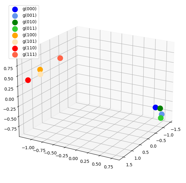
(a) $\widehat{\mathcal{D}}=\{(0,\diamond,\diamond),(1,\diamond,\diamond)\}$

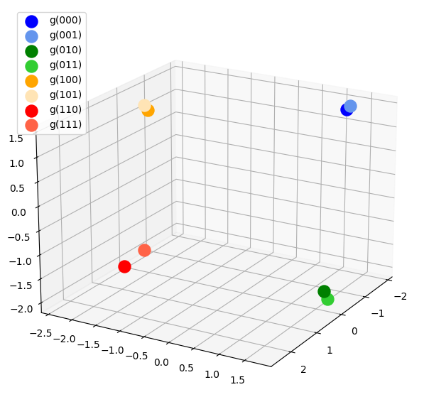
(b) $\widehat{\mathcal{D}}=\{(0,0,\diamond),(0,1,\diamond),(1,0,\diamond),(1,1,\diamond)\}$

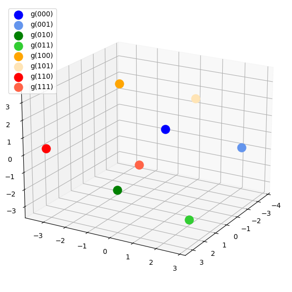
(c) $\widehat{\mathcal{D}}=\mathcal{D}$

Figure 2: Unembedding representations form different clusters after training on various conditioning sets. This figure shows unembedding representations after learning different sets of conditional distributions.

While stated generally as a result of the properties of gradient descent, Theorem 5 says that when the latent conditional models are trained on a subproblem of next token prediction with reasonable initializations (see below remark), implicit bias of gradient descent will align the embedding and unembedding vectors as well as aligning among the unembedding vectors. This can manifest as linear representations in the final trained LLMs such as LLaMA-2 [Tou+23]. Although the theorem addresses only a specific subproblem, it notably suggests, as discussed earlier, the underlying bias and dynamics that contribute to the emergence of linear representations. That is, if one solely optimizes this subproblem, one can get perfect linear representations. We verify this result empirically in Section 5.

Remark 6.

The initial condition assumption in the theorem statement seems unnecessary as evidenced by our experiments in Section 5. On the other hand, if one initializes vectors with high dimensional multivariate Gaussians, then the assumption will be approximately satisfied with high probability [Das99].

The role of learning various conditional distributions

So far, we have only discussed learning conditional distributions for a single concept. In general, due to the presence of zero probabilities in various conditioning contexts, learning these conditional probabilities is, in some sense, learning different forces to push sets of representations far apart because one needs relatively large inner products to get exponents to be close to zero.

Fig. 2 gives an illustrative example with three concept variables that shows how learning different subsets of conditional probabilities would push various subsets of unembeddings in different ways. For example, if the model exclusively learns conditional probabilities for $C_{1}$, the unembedding representations would form clusters based on the values of $C_{1}$. Similarly, if the model learns conditional probabilities for both $C_{1}$ and $C_{2}$, the unembedding representations would cluster based on the values of both $C_{1}$ and $C_{2}$. However, in the second case, the concept directions of $C_{1}$ and $C_{2}$ are coupled. As shown in Fig. 2(b), $g(110)-g(100)$ is parallel with $g(111)-g(101)$ but not with $g(010)-g(000)$. To decouple them, one needs a bigger $\widehat{\mathcal{D}}$ as in Fig. 2(c). That said, it seems that a complete set of $\mathcal{D}$ is not always necessary (Section 5).

An analogy would be to view each binary vector as a combination of “electrons” where the values represent positive or negative charges. Learning probabilities under different conditioning contexts can be likened to applying various forces to manipulate the positions of these electrons. This is similar to the Thomson Problem in chemistry and occurs in other contexts of representation learning as well [Elh+22].

4 Orthogonality

A surprising phenomenon observed in LLMs like LLaMA-2 [Tou+23] is that the Euclidean geometry can somewhat capture semantic structures, despite the fact that the Euclidean inner product is not identified by the training objective [PCV23]. Consequently, one notable outcome is the tendency for semantically unrelated concepts to be represented as almost orthogonal vectors in the unembedding space. In this section, we study this phenomenon under our latent conditional model. Based on our underlying Markov random field distribution, we define unrelated concepts to be those separated in $G_{C}$.

Theorem 7.

Let $\widehat{\mathcal{C}}=\mathcal{C}$ and $\widehat{\mathcal{D}}=\mathcal{D}$. Assuming $p(c)>0$ for any $c\in\mathcal{C}$ and $C_{i}$ and $C_{j}$ are two latent variables separated in $G_{C}$. Given any binary vector $c\in\mathcal{C}$, there exists a subset $\mathcal{D}_{c}\subset\mathcal{D}$ such that $d_{i}=\diamond$ and ${p}(c|d)>0$ for any $d\in\mathcal{D}_{c}$. If one further assume that $\hat{p}(c|d)={p}(c|d)$ for any $d\in\mathcal{D}_{c}$, then

$$g(c_{(i\to 1)})-g(c_{(i\to 0)})\perp f(d_{(j\to c_{j})})-f(d_{(j\to\diamond)})$$

for any $d\in\mathcal{D}_{c}$.

All proofs are deferred to Appendix D. As suggested in Section 3.2 and verified empirically in Section 5, under the latent conditional model, representations are not only linearly encoded but also frequently aligned between embedding and unembedding spaces, which implies the following corollary on the orthogonal representation of unrelated concepts.

Corollary 8.

Under the conditions of Theorem 7, if concept $C_{i}$ and $C_{j}$ have matched-representations, then

$$g(c_{(i\to 1)})-g(c_{(i\to 0)})\perp g(c_{(j\to 1)})-g(c_{(j\to 0)})$$

for any $c\in\mathcal{C}$.

In simulation, given enough dimensions, the latent conditional model tends to learn near orthogonal representations regardless of graphical dependencies. One plausible rationale behind this phenomenon is the tendency for steering vectors in both unembedding and embedding spaces to possess large norms because, by Proposition 11, the inner product of embedding and unembedding steering vectors of the same concept is large. However, for steering vectors representing distinct concepts, it’s often necessary for the inner product to be small as dictated by what’s given in the training distributions. To accommodate for this, their cosine similarities tend to be close to zero. As a consequence, unembedding representations of different concepts often end up being near orthogonal as well.

Remark 9.

It is worth noting that the conditions for orthogonal representations presented here can break in practice for LLMs. For instance, the injectivity assumption might not hold, and embedding and unembedding representations might not have perfectly matched representations.

5 Experiments

In this section, we present two slates of experiments to validate and augment our theoretical contributions. Specifically, in Section 5.1, we run experiments on simulated data from the latent conditional model to verify the existence of linear and orthogonal representations in this theoretical framework and how training on smaller dimensions, incomplete sets of contexts, and concept vectors can affect the representations. Then, we run experiments on large language models in Section 5.2 to show nontrivial alignment between embedding and unembedding representations of the same concept as predicted by our theory.

5.1 Simulated experiments

Simulation setup

For simulation experiments, we first create simulated datasets by initially creating random DAGs (see Remark 1) with $m$ variables/concepts. For a specific random DAG, the conditional probabilities of one variable given its parents are modeled by Bernoulli distributions where the parameters are sampled uniformly from $[0.3,0.7]$. For example, suppose the DAG is $C_{1}\to C_{2}$. Then $C_{1}\sim\mathrm{Bern}(p_{1})$, $(C_{2}|C_{1}=0)\sim\mathrm{Bern}(p_{2})$, $(C_{2}|C_{1}=1)\sim\mathrm{Bern}(p_{3})$ where $p_{1},p_{2},p_{3}\sim\mathrm{Unif}\leavevmode\nobreak\ ([0.3,0.7])$. In other words, we generate random graphical models wherein both the structures and distributions are created randomly. From these random graphical models, we can sample values of variables which are binary vectors as our datasets.

To let models learn conditional distributions, we train them to make predictions under cross-entropy loss after randomly masking the sampled binary vectors. Unless otherwise stated, the model is trained using stochastic gradient descent with a learning rate of $0.1$ and batch size $100$. More details are deferred to Appendix E.

Complete set of conditionals ($\widehat{\mathcal{C}}=\mathcal{C},\widehat{\mathcal{D}}=\mathcal{D}$)

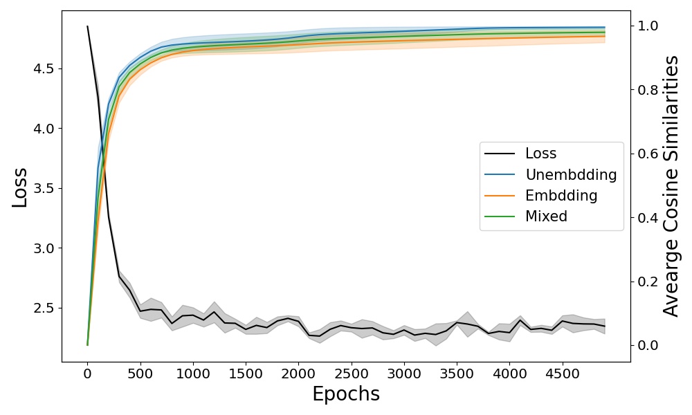
Figure 5: Loss and cosine similarities change as training progresses. The experiments are tested with $7$ hidden variables over 10 runs.

We first run experiments where the model is trained to learn the complete set of conditional distributions. The representation dimension is set to be the same as the number of latent variables. Given a concept, to measure linearity, we calculate the average cosine similarities among steering vectors in the unembedding space and in the embedding space as well as between steering vectors in these two spaces. The result is shown in Table 1 which suggests that under the latent conditional model with the complete set of contexts, learned representations are indeed linearly encoded. In addition, Fig. 5 in Appendix E shows that as loss decreases, the cosine similarities increase rapidly. Due to the exponential number of vectors that need to be trained, one cannot directly simulate a large number of latent variables. However, as we will show later (Appendix E), one can use incomplete sets $\widehat{\mathcal{C}}$ and $\widehat{\mathcal{D}}$ and simulate with more latent variables.

Table 1: When the model is trained to learn the complete set of conditionals, the $m$ latent variables are represented linearly, and the embedding and unembedding representations are matched. The table shows average cosine similarities among and between steering vectors of unembeddings and embeddings. Standard errors are over $100$ runs for $3$ variables and $4$ variables, $50,20$ and $10$ runs for $5,6$ and $7$ variables respectively.

$m$	Unembedding	Embedding	Unembedding and Embedding
3	0.972$\pm$0.006	0.982$\pm$0.005	0.980$\pm$0.005
4	0.975$\pm$0.005	0.971$\pm$0.005	0.973$\pm$0.005
5	0.988$\pm$0.004	0.981$\pm$0.004	0.984$\pm$0.004
6	0.997$\pm$0.000	0.985$\pm$0.002	0.990$\pm$0.001
7	0.995$\pm$0.001	0.972$\pm$0.004	0.981$\pm$0.003

Orthogonality

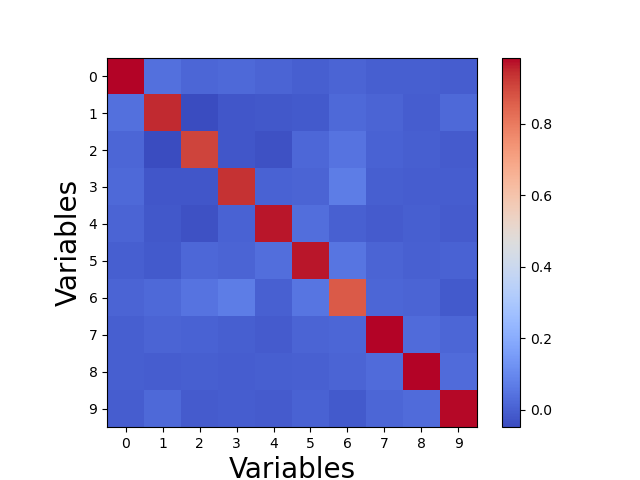
(a) Simulated Experiments

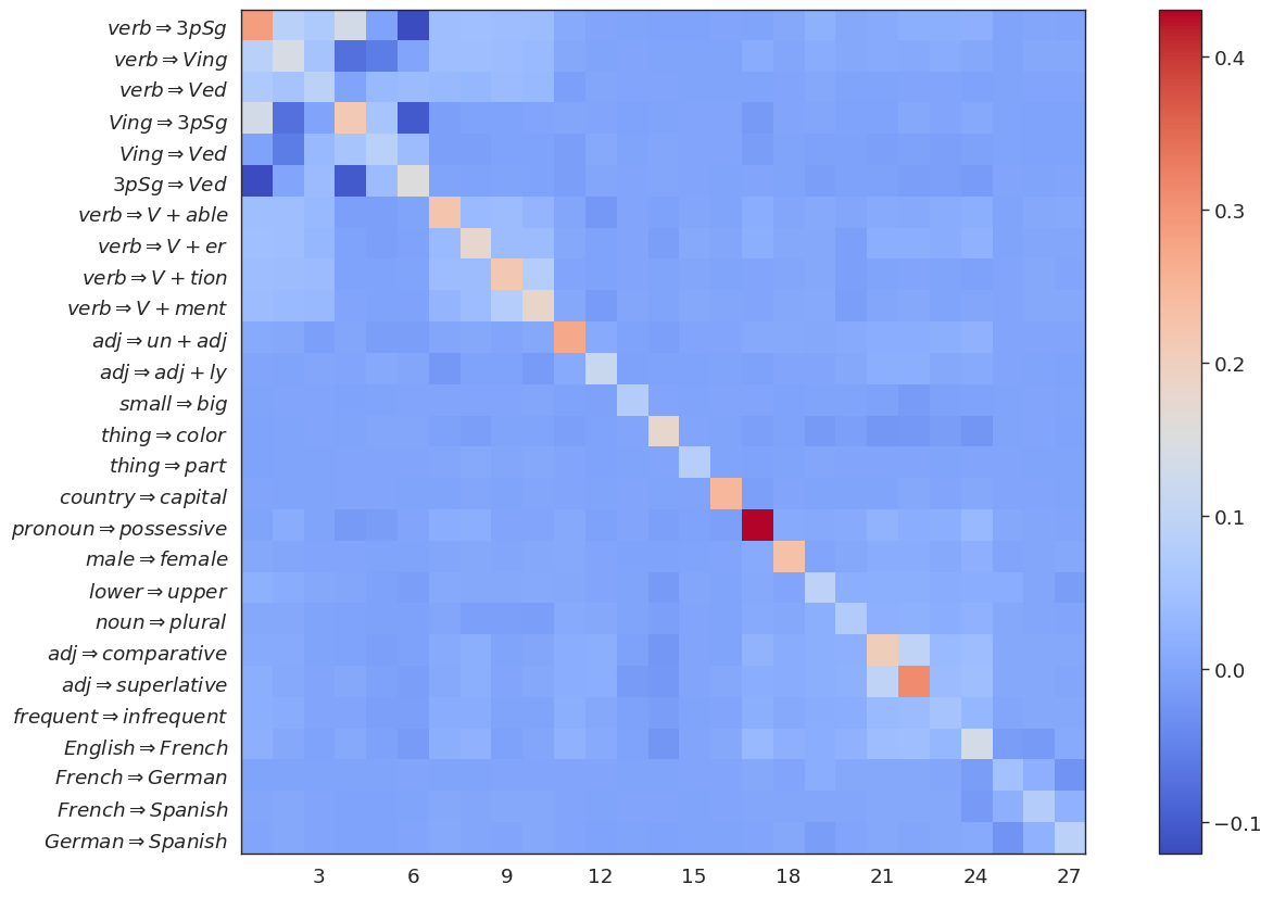
(b) LLaMA-2

Figure 7: The pattern of linear and orthogonal representations matches between simulated experiments and LLaMA-2. Specifically, unembedding steering vectors of the same concept in LLaMA-2 have nontrivial alignment, while steering vectors of different concepts are represented almost orthogonally. The heatmap shows the average cosine similarities between different sets of steering vectors for both simulated experiments and LLaMA-2. For simulated experiments, the cosine similarities are averaged over $10$ runs.

Section 4 argues that, under the latent conditional model, unembedding representations of separated concepts will be orthogonal. In practice, Fig. 7(a) (Appendix E) shows that this happens for simulated data even without latent variables being separated in the latent graph. We test the orthogonalities of representations in the latent conditional model by calculating the average cosine similarities between different sets of steering vectors. To see how well the theoretical framework fits LLMs, we similarly calculate the average cosine similarities between different sets of steering vectors in LLaMA-2 [Tou+23] using the counterfactual pairs in [PCV23] and they’re reported in Fig. 3. In particular, Fig. 7 (Appendix E) shows that both simulated experiments and LLaMA-2 experiments exhibit similar behaviors where steering vectors of the same concept are more aligned while steering vectors of different concepts are almost orthogonal. This validates the claim that the latent conditional model is a suitable proxy to study LLMs.

In real-life datasets, not every concept or context vector has a natural correspondence to a token or sentence. On the other hand, the number of tokens and sentences grows exponentially with the number of latent concepts. Therefore, it is not realistic to always have $\widehat{\mathcal{D}}=\mathcal{D}$ or $\widehat{\mathcal{C}}=\mathcal{C}$. In other words, one does not need the next token prediction to learn all possible conditional probabilities perfectly. Because we are in a simulated setup, it’s easy to probe the behavior in these situations. Therefore, we also perform additional experiments to observe these aspects of our simulated setup, in particular (i) Training on an incomplete set of contexts ($\widehat{\mathcal{D}}\subset\mathcal{D}$), (ii) Incomplete set of concept vectors ($\widehat{\mathcal{C}}\subset\mathcal{C}$). These are deferred to Appendix E. The experiments show that linearity is robust to these changes.

Moreover, in practice, the representation dimension is typically much smaller than the number of concepts represented. Thus, we run additional experiments in Appendix E with decreasing dimensions and observe one can still get reasonable linear representations.

Finally, we show in Appendix E that gradient descent or stochastic gradient descent is not the only algorithm that can induce linear representation, running other first-order methods like Adam [KB15] can lead to a similar pattern.

Figure 3: Unembedding steering vectors of the same concept in LLaMA-2 have nontrivial alignment, but steering vectors of different concepts are represented almost orthogonally.

5.2 Experiments with large language models

In this section, we will conduct experiments on pre-trained large language models. We first emphasize that prior works [Elh+22, Bur+22, Tig+23, NLW23, Mos+22, PCV23, Gur+23] have already exhibited certain geometries of LLM representations related to linearity and orthogonality, via experiments. Therefore, in this section, we probe the geometry of the LLM representations, in particular that of the interplay between the embeddings and unmbeddings of the contexts and the tokens, that have not been explored in prior works. As [PCV23] remark, for a given binary concept, it’s hard to generate pairs of contexts that differ in precisely this context, partly because of nuances of natural language and mainly because such counterfactual sentences are hard to construct even for human beings. In this section, we try to recreate these sets of missing experiments in the literature using existing open-source datasets.

Multilingual embedding geometry

We first consider language translation concepts. For the embedding vectors, we consider pairs of contexts $(x^{0},x^{1})$ where $x^{0},x^{1}$ are the same sentences but in different languages. We consider four language pairs French–Spanish, French–German, English–French, and German–Spanish from the OPUS Books dataset [Tie12]. We take 150 random samples and filter out contexts with less than 20 or more than 150 tokens. For the unembedding concept vectors, we use the 27 concepts as described in [PCV23], which were built on top of the Big Analogy Test dataset [GDM16]. Examples of both datasets and a list of the 27 concepts are shown in Appendix F.

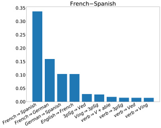
Figure 4: The French–Spanish concept is highly correlated with similar token concepts relative to others. Figure shows cosine similarities between the French–Spanish concept and token concepts.

We consider embeddings and unembeddings from LLaMA-2-7B [Tou+23]. We compute the absolute cosine similarity between the average embedding steering vector and the average unembedding steering vector. A barplot for French–Spanish with top 10 similarities is shown in Fig. 4. The entire barplot with 27 concepts and the barplots for the other language translation concepts are in Appendix F. As we can see, there is alignment between the embedding and unembedding representations for matching concepts relative to unmatched concepts, as Theorem 5 predicts.

Winograd Schema

Next, we consider counterfactual context pairs arising from the Winograd Schema dataset [LDM12], which is a dataset of pairs of sentences that differ in only one or two words and which further contain an ambiguity that can only be resolved with world knowledge and reasoning. We run experiments similar to the multilingual embedding geometry experiments and also run additional experiments on similarities between Winograd context pairs and the 27 concepts from [PCV23]. The experiment details are in Appendix F.

These LLM experiments show that matching contexts are better aligned with the corresponding unembedding steering vectors than non-matching contexts, as predicted from our theory. Note that although the final cosine similarities are lower than what was exhibited in the simulated experiments, this is not surprising due to the complexity and nuances of natural language and LLMs. Another reason is that abstract concepts do not necessarily lie in a one-dimensional space, so standard cosine similarity metrics may not be an optimal choice here. However, the partial alignment already serves to strongly validate our theoretical insights.

6 Literature review

Linear representations

Linear representations have been observed empirically in word embeddings [MYZ13, PSM14, Aro+16] and large language models [Elh+22, Bur+22, Tig+23, NLW23, Mos+22, PCV23, Gur+23]. Many works in the pre-LLM era, also attempt to explain this phenomenon theoretically. For instance, [Aro+15] and their follow-up works [Aro+18, FG19] study the RAND-WALK model in which latent vectors undergo continuous drift on the unit sphere. A similar notion can be found also in dynamic topic modeling [BL06] and its subsequent works [Rud+16, RB17]. In contrast, the latent conditional model in this paper studies discrete latent concept variables that can capture semantic meanings.

Other works include the paraphrasing model [GAM17, AH19, ABH19], which proposes to study a subset of words that are semantically equivalent to a single word, however the uniformity assumption is somewhat unrealistic. [EDH18] explore how the linearity property can arise by decomposing pointwise mutual information matrix and [RLV23] examine the phenomenon from the perspective of contrastive loss which all rely on assumptions on the matching of probability ratios.

wang2023concept also use a latent variable model between prompt and output to establish the linear structure of representations. However, they study this phenomena in the context of text-to-image diffusion models, and their construction relies heavily on the Stein score representation. By contrast, the model here is closer to the standard decoder-only LLM setup, and highlights the key role of softmax.

Linearity has also been observed in other domains such as computer vision [RMC15, Rag+17, Bau+17, EHR17, Kim+18, Tra+23, Wan+23] and other intelligent systems [McG+22, Sch+23]. We expect our ideas to extend to other domains, however we restrict our attention to language modeling in this work.

Geometry of representations

There’s a body of work on studying the geometry of word and sentence representations [MT17, Rei+19, VM21, VM20, Li+20, Che+21, CTB22, Lia+22, JAV23, PCV23]. In particular, [MT17] and [Lia+22] discover representation gaps in the context of word embeddings and vision-language models. [PCV23] attempts to define a suitable inner product that captures semantic meanings. [JAV23] study the connection between independence and orthogonal representation by adopting the abstract notion of independence models. One can also view embeddings in the context of information geometry [VM21, VM20].

Causal representation learning

There is a subtle connection between our work and the field of causal representation learning that we now briefly comment on. Causal representation learning [Sch+21, SK22] is an emerging field that exploits ideas from the theory of latent variable modeling [Aro+13, Kiv+21, HKM23] along with causality [SGS00, Pea09, Raj+21, SU22] to build generative models for various domains. The main goal is to build the true generative models that led to the creation of a dataset. This field has made exciting advances in recent years [Khe+20, Fal+21, Zim+21, Kiv+22, Lac+22, Raj+23, Var+23, Raj+24, JA23, Buc+23, HKM23]. However, to study large foundation models, a purely statistical notion of building the true model may not reflect the entire story as one should also take into account the implicit bias of optimization as well (Section 3.2). Moreover, identifying the entire underlying latent distributions may also not be necessary for certain practical purposes and it might be sufficient to represent only certain structure information in the geometry of representations, such as linearly encoded representations. Another example of this has been recently explored by [JAV23] namely independence preserving embedding which studies how independence structure can be stored in representations.

7 Conclusion

In this work, we presented a simple latent variable model and showed that using a standard LLM pipeline to learn the distribution results in concepts being linearly represented. We observed that this linear structure is promoted in (at least) two ways—(i) matching log-odds, similar to prior works on word embeddings, and (ii) implicit bias of gradient descent. Additionally, experimental results show that—as predicted—the linear structure emerges from the simple latent variable model. We also saw that, as predicted in the simple model, LLaMA-2 representations exhibit alignment between embedding and unembedding representations.

Acknowledgements

This work is supported by ONR grant N00014-23-1-2591, Open Philanthropy, NSF IIS-1956330, NIH R01GM140467, and the Robert H. Topel Faculty Research Fund at the University of Chicago Booth School of Business. We also acknowledge the support of AFRL and DARPA via FA8750-23-2-1015, ONR via N00014-23-1-2368, and NSF via IIS-1909816, IIS-1955532.

Appendix A Linearity from log-odds: Proof of Theorem 3

In this section, we prove Theorem 3 restated below for convenience.

See 3

Proof.

Fix any $i\leq m$ and consider the vector $\overline{\Delta_{c,i}}=\Pi_{i}(g(c_{(i\to 0)})-g(c_{(i\to 1)}))$ for any $c\in\mathcal{C}$. Let $\widehat{\mathcal{D}}=\{d\in\{\diamond,0,1\}^{m}|d_{i}=\diamond\}$ be the contexts that do not condition on $C_{i}$ and let $u_{1},\ldots,u_{k}$ be an orthonormal basis of the space $\text{span}\{f(d)|d\in\widehat{\mathcal{D}}\}$. Also, since $f(d)$ over $d\in\widehat{\mathcal{D}}$ span this space, let

$$u_{j}=\sum_{d\in\widehat{\mathcal{D}}}\alpha_{j,d}f(d)$$

for all $j=1,2,\ldots,k$ and scalars $\alpha_{j,d}$. Note that the $\alpha_{j,d}$ do not depend on $c$. Now, for any $j\leq k$,

$$\langle\overline{\Delta_{c,i}},u_{j}\rangle =\langle\Pi_{i}(g(c_{(i\to 0)})-g(c_{(i\to 1)})),u_{j}\rangle$$

$$=\langle g(c_{(i\to 0)})-g(c_{(i\to 1)}),\Pi_{i}u_{j}\rangle$$

$$=\langle g(c_{(i\to 0)})-g(c_{(i\to 1)}),u_{j}\rangle$$

$$=\langle g(c_{(i\to 0)})-g(c_{(i\to 1)}),\sum_{d\in\mathcal{D}}\alpha_{j,d}f(d)\rangle$$

$$=\sum_{d\in\widehat{\mathcal{D}}}\alpha_{j,d}\langle g(c_{(i\to 0)})-g(c_{(i\to 1)}),f(d)\rangle$$

To this end, we will compute the inner product $\langle g(c_{(i\to 0)})-g(c_{(i\to 1)}),f(d)\rangle$ for a fixed $d\in\widehat{\mathcal{D}}$. First,

$$\ln\frac{\hat{p}(c_{(i\to 0)}|d)}{\hat{p}(c_{(i\to 1)}|d)}=\ln\frac{p(C_{i}=0)}{p(C_{i}=1)}$$

But we have

$$\hat{p}(c_{(i\to 0)}|d)=\frac{\exp(f(d)^{T}g(c_{(i\to 0)}))}{\sum_{c^{\prime}}\exp(f(d)^{T}g(c^{\prime}))},\qquad\hat{p}(c_{(i\to 1)}|d)=\frac{\exp(f(d)^{T}g(c_{(i\to 1)}))}{\sum_{c^{\prime}}\exp(f(d)^{T}g(c^{\prime}))}$$

Since the denominator does not depend on $c$, rearranging implies

$$\langle g(c_{(i\to 0)})-g(c_{(i\to 1)}),f(d)\rangle =f(d)^{T}(g(c_{(i\to 1)})-g(c_{(i\to 0)}))$$

$$=\ln\frac{\hat{p}(c_{(i\to 0)}|d)}{\hat{p}(c_{(i\to 1)}|d)}$$

$$=\ln\frac{p(C_{i}=0)}{p(C_{i}=1)}$$

which only depends on $i$. Call this expression $\alpha^{(i)}$ to get

$$\langle\overline{\Delta_{c,i}},u_{j}\rangle =\sum_{d\in\widehat{\mathcal{D}}}\alpha_{j,d}\langle g(c_{(i\to 0)})-g(c_{(i\to 1)}),f(d)\rangle$$

$$=\sum_{d\in\widehat{\mathcal{D}}}\alpha_{j,d}\alpha^{(i)}$$

Therefore,

$$\overline{\Delta_{c,i}} =\sum_{j\leq k}\langle\overline{\Delta_{c,i}},u_{j}\rangle u_{j}$$

$$=\sum_{j\leq k}\left(\sum_{d\in\widehat{\mathcal{D}}}\alpha_{j,d}\alpha^{(i)}\right)u_{j}$$

$$=\alpha^{(i)}\sum_{j\leq k,d\in\widehat{\mathcal{D}}}\alpha_{j,d}u_{j}$$

Note that regardless of $c$, the final expression is always parallel to the vector $v_{i}=\sum_{j\leq k,d\in\widehat{\mathcal{D}}}\alpha_{j,d}u_{j}$ which does not depend on $c$. This completes the proof. ∎

Appendix B Linearity from log-odds for general MRFs

In this section, we generalize the ideas from Appendix A to concepts from a general Markov random field, which is more general than the independent case. Since most of the technical ideas and motivations are in Appendix A, we will go over them lightly here. The goal is to study the structure of the steering vector $\Delta_{c,i}=g(c_{(i\to 1)})-g(c_{(i\to 0)})$. As we will see, instead of them all lying in a space of dimension $1$ as in the independent case (that’s what being parallel means), they will now live in a subspace of low dimension. For example, such a phenomenon was experimentally observed by [Li+23] for the concept of truthfulness.

Here, concepts $C_{1},\ldots,C_{m}$ come from a Markov random field with undirected graph $G_{C}=(V_{C},E_{C})$ with neighborhood set given by $\textrm{ne}(i)$. Therefore, they satisfy the property that $p(C_{i}|C_{[m]\setminus i})=p(C_{i}|C_{\textrm{ne}(i)})$ for all $i\leq m$. Accordingly, we state the log-odds assumption to capture this general conditional independence.

Assumption 1.

For any concept $i\leq m$, any concept vector $c\in\mathcal{C}$ and context $d\in\{\diamond,0,1\}^{m}$ such that $d_{i}=\diamond$ and $d_{j}\neq\diamond$ for all $j\in\textrm{ne}(i)$, we have

$$\ln\frac{\hat{p}(c_{(i\to 0)}|d)}{\hat{p}(c_{(i\to 1)}|d)}=\ln\frac{p(C_{i}=0|C_{\textrm{ne}(i)}=d_{\textrm{ne}(i)})}{p(C_{i}=1|C_{\textrm{ne}(i)}=d_{\textrm{ne}(i)})}$$

As before, we assume above that the log odds condition holds when $i$ is not conditioned on, but we weaken this further to say that it only needs to hold specifically when every one of its neighbors $j$ has been conditioned on.

Analogously, we project out the space that could possibly contribute to a $0$ conditional probability. This is the space where either $d_{i}$ has been conditioned on or $d_{j}$ for some $j\in\textrm{ne}(i)$ has been conditioned on. Therefore, define $\overline{\Delta_{c,i}}=\Pi_{i}\Delta_{c,i}$ where $\Pi_{i}$ is the projection into the space $\text{span}\{f(d)|d_{i}=\diamond,d_{j}\neq\diamond\forall j\in\textrm{ne}(i)\}$ We now state our main theorem.

Theorem 10.

Under Assumption 1, for any fixed $i\leq m$, the vectors $\overline{\Delta_{c,i}}$ for all $c\in\mathcal{C}$ live in a subspace $\mathcal{S}$ of dimension at most $2^{|\textrm{ne}(i)|}$.

This theorem says that if we assume that the concepts come from a general Markov random field, then the steering vectors live in a space of low dimension. Note that when the concepts are independent, we have $|\textrm{ne}(i)|=0\Longrightarrow 2^{|\textrm{ne}(i)|}=1$ which means all the vectors $\overline{\Delta_{c,i}}$ are parallel. Therefore this theorem is more general than Theorem 3.

Proof.

We will proceed similarly to the proof of Theorem 3. Fix any $i\leq m,c\in\mathcal{C}$ and repeat the computation until we get that for any $j\leq k$,

$$\langle\overline{\Delta_{c,i}},u_{j}\rangle =\sum_{d\in\widehat{\mathcal{D}}}\alpha_{j,d}\langle g(c_{(i\to 0)})-g(c_{(i\to 1)}),f(d)\rangle$$

where $\widehat{\mathcal{D}}=\{d\in\{\diamond,0,1\}^{m}|d_{i}=\diamond,d_{j}\neq\diamond\forall j\in\textrm{ne}(i)\}$. Now, let’s recompute $\langle g(c_{(i\to 0)})-g(c_{(i\to 1)}),f(d)\rangle$. By Assumption 1, we have

$$\ln\frac{\hat{p}(c_{(i\to 0)}|d)}{\hat{p}(c_{(i\to 1)}|d)}=\ln\frac{p(C_{i}=0|C_{\textrm{ne}(i)}=d_{\textrm{ne}(i)})}{p(C_{i}=1|C_{\textrm{ne}(i)}=d_{\textrm{ne}(i)})}$$

which gives

$$\langle g(c_{(i\to 0)})-g(c_{(i\to 1)}),f(d)\rangle =\ln\frac{p(C_{i}=0|C_{\textrm{ne}(i)}=d_{\textrm{ne}(i)})}{p(C_{i}=1|C_{\textrm{ne}(i)}=d_{\textrm{ne}(i)})}$$

which depends both on $i$ and $d_{\textrm{ne}(i)}$. For all $\sigma\in\{0,1\}^{|\textrm{ne}(i)|}$, denote $\alpha^{(i),\sigma}$ to be the expression

$$\alpha^{(i),\sigma} =\ln\frac{p(C_{i}=0|C_{\textrm{ne}(i)}=\sigma)}{p(C_{i}=1|C_{\textrm{ne}(i)}=\sigma)}$$

Therefore,

$$\overline{\Delta_{c,i}} =\sum_{j\leq k}\left(\sum_{d\in\widehat{\mathcal{D}}}\alpha_{j,d}\alpha^{(i),d_{\textrm{ne}(i)}}\right)u_{j}$$

$$=\sum_{\sigma\in\{0,1\}^{|\textrm{ne}(i)|}}\alpha^{(i),\sigma}\left(\sum_{j\leq k,d\in\widehat{\mathcal{D}},d_{\textrm{ne}(i)}=\sigma}\alpha_{j,d}u_{j}\right)$$

which lives in the span of the vectors $v^{(i),\sigma}=\sum_{j\leq k,d\in\widehat{\mathcal{D}},d_{\textrm{ne}(i)}=\sigma}\alpha_{j,d}u_{j}$ regardless of $c$. The number of such vectors is $|\{0,1\}^{|\textrm{ne}(i)|}|=2^{|\textrm{ne}(i)|}$. ∎

Appendix C Linearity from the implicit bias of gradient descent

In this section, we will prove Theorem 4 and Theorem 5 and additional auxiliary theorems.

See 4

Proof.

First note that we can break the whole optimization problem into smaller subproblems where each subproblem only depends on one counterfactual pair. By Theorem 3 of [Sou+18], all $\Delta_{c,i}$ converges to have the same direction as the hard margin SVM solution. ∎

Proposition 11.

Suppose $p(c)>0$ for any $c\in\widehat{\mathcal{C}}=\mathcal{C}$ and $|\hat{p}(c|d)-p(c|d)|<\varepsilon$ for all $c\in\widehat{\mathcal{C}}$ and $d\in\widehat{\mathcal{D}}$ such that $0<\varepsilon<p(c|d)$ for all $c,d$ where $p(c|d)>0$. Then for any latent variable $C_{i}$, we have that

$$\exp(-(g(c_{(i\to 1)})-g(c_{(i\to 0)}))^{T}(f(d_{(i\to 0)})-f(d_{(i\to 1)})))<\frac{\varepsilon^{2}}{\big{(}p(c_{c_{i}=0}|d_{c_{i}=0})-\varepsilon\big{)}\big{(}p(c_{c_{i}=1}|d_{c_{i}=1})-\varepsilon\big{)}}$$

for any $c\in\widehat{\mathcal{C}}$ and any $d\in\widehat{\mathcal{D}}$.

Proof.

For any $c\in\widehat{\mathcal{C}}$ and $d\in\widehat{\mathcal{D}}$, we have that

$$\begin{split}\frac{p(c_{c_{i}=1}|d_{c_{i}=0})}{p(c_{c_{i}=0}|d_{c_{i}=0})}=0,\qquad\frac{p(c_{c_{i}=0}|d_{c_{i}=1})}{p(c_{c_{i}=1}|d_{c_{i}=1})}=0\end{split}$$

These ratios are well-defined because $p(c)>0$ for any $c$. Therefore,

$$\begin{split}\frac{\hat{p}(c_{c_{i}=1}|d_{c_{i}=0})}{\hat{p}(c_{c_{i}=0}|d_{c_{i}=0})}<\frac{\varepsilon}{p(c_{c_{i}=0}|d_{c_{i}=0})-\varepsilon},\qquad\frac{\hat{p}(c_{c_{i}=0}|d_{c_{i}=1})}{\hat{p}(c_{c_{i}=1}|d_{c_{i}=1})}<\frac{\varepsilon}{p(c_{c_{i}=1}|d_{c_{i}=1})-\varepsilon}\end{split}$$

Thus,

$$\begin{split}\exp(-(g(c_{(c_{i}=1)})&-g(c_{(c_{i}=0)}))^{T}(f(d_{(c_{i}=0)})-f(d_{(c_{i}=1)})))\\ &=\frac{\hat{p}(c_{c_{i}=1}|d_{c_{i}=0})}{\hat{p}(c_{c_{i}=0}|d_{c_{i}=0})}\frac{\hat{p}(c_{c_{i}=0}|d_{c_{i}=1})}{\hat{p}(c_{c_{i}=1}|d_{c_{i}=1})}<\frac{\varepsilon^{2}}{\big{(}p(c_{c_{i}=0}|d_{c_{i}=0})-\varepsilon\big{)}\big{(}p(c_{c_{i}=1}|d_{c_{i}=1})-\varepsilon\big{)}}\end{split}$$

∎

Theorem 12.

Given loss function $L(u,v)=\exp(-u^{T}v)$, any starting point $u_{0},v_{0}$ where $u_{0}\neq-\alpha v_{0}$ for some $\alpha>0$, and any step size $\eta<\frac{1}{L(u_{0},v_{0})}$, the gradient descent iterates will have the following properties:

1. $\lim_{t\to\infty}L(t)=\lim_{t\to\infty}L(u_{t},v_{t})=0$

2. $\lim_{t\to\infty}||u_{t}||\to\infty$ and $\lim_{t\to\infty}||v_{t}||\to\infty$

3. $\cos(u_{t},v_{t})$ increases monotonically with $t$

4. $\lim_{t\to\infty}\cos(u_{t},v_{t})=1$

Proof.

Before proving the theorem, let’s write out a few equations. By the gradient descent algorithm, we have the following equations:

$$\begin{split}u_{t+1}&=u_{t}+\eta L(t)v_{t}\\ v_{t+1}&=v_{t}+\eta L(t)u_{t}\end{split}$$

Thus,

$$\begin{split}||u_{t+1}||^{2}&=||u_{t}||^{2}+2\eta L(t)\langle u_{t},v_{t}\rangle+\eta^{2}L(t)^{2}||v_{t}||^{2}\\ ||v_{t+1}||^{2}&=||v_{t}||^{2}+2\eta L(t)\langle u_{t},v_{t}\rangle+\eta^{2}L(t)^{2}||u_{t}||^{2}\\ \langle u_{t+1},v_{t+1}\rangle&=(1+\eta^{2}L(t)^{2})\langle u_{t},v_{t}\rangle+\eta L(t)(||u_{t}||^{2}+||v_{t}||^{2})\end{split}$$

Now let’s prove each claim one by one.

First of all, we know that

$$\langle u_{t+1},v_{t+1}\rangle-\langle u_{t},v_{t}\rangle=\eta^{2}L(t)^{2}\langle u_{t},v_{t}\rangle+\eta L(t)(||u_{t}||^{2}+||v_{t}||^{2})$$

The difference is positive if $\langle u_{t},v_{t}\rangle>0$. To deal with the case of a negative inner product, we will use induction to prove that for any $t$, $\langle u_{t+1},v_{t+1}\rangle-\langle u_{t},v_{t}\rangle$ is positive and thus $L(t)$ decreases monotonically.

Base case ($t=0$): The difference is positive if $\langle u_{0},v_{0}\rangle>0$. Let’s consider the case when $\langle u_{0},v_{0}\rangle\leq 0$

$$\begin{split}\langle u_{1},v_{1}\rangle-\langle u_{0},v_{0}\rangle&=\eta^{2}L(0)^{2}\langle u_{0},v_{0}\rangle+\eta L(0)(||u_{0}||^{2}+||v_{0}||^{2})\\ &=(\eta^{2}L(0)^{2}-2\eta L(0))\langle u_{0},v_{0}\rangle+\eta L(0)(u_{0}+v_{0})^{2}\\ &=\eta L(0)(\eta L(0)-2)\langle u_{0},v_{0}\rangle+\eta L(0)(u_{0}+v_{0})^{2}>0\end{split}$$

The last inequality is due to $\eta<\frac{1}{L(u_{0},v_{0})}$.

Inductive step : Again, the difference is positive if $\langle u_{t},v_{t}\rangle>0$. Let’s consider the case when $\langle u_{t},v_{t}\rangle\leq 0$

$$\begin{split}\langle u_{t+1},v_{t+1}\rangle-\langle u_{t},v_{t}\rangle&=\eta^{2}L(t)^{2}\langle u_{t},v_{t}\rangle+\eta L(t)(||u_{t}||^{2}+||v_{t}||^{2})\\ &=(\eta^{2}L(t)^{2}-2\eta L(t))\langle u_{t},v_{t}\rangle+\eta L(t)(u_{t}+v_{t})^{2}\\ &=\eta L(t)(\eta L(t)-2)\langle u_{t},v_{t}\rangle+\eta L(t)(u_{t}+v_{t})^{2}>0\end{split}$$

The last inequality is due to $\eta<\frac{1}{L(u_{0},v_{0})}$ and the inductive hypothesis that $L(t)$ decreases monotonically.

It is worth noting because $\langle u_{t},v_{t}\rangle$ is monotonically increasing, there must exist a time $t_{p}$ such that $\langle u_{t_{p}},v_{t_{p}}\rangle>0$. If the opposite is true, then $\langle u_{t},v_{t}\rangle$ must converge to a nonpositive number which is not possible because the difference between consecutive numbers in the sequence is strictly positive unless both $u_{t}$ and $v_{t}$ converges to zero. In other words, if $\langle u_{t},v_{t}\rangle$ does not diverge, it must be a Cauchy sequence which needs both $u_{t}$ and $v_{t}$ to reach $0$. Suppose $u_{t}\to 0$ and $v_{t}\to 0$. We know that

$$u_{t+1}+v_{t+1}=(1+\eta L(t))(u_{t}+v_{t})$$ (C.1)

which means the only possible scenario that $u_{t}\to 0$ and $v_{t}\to 0$ is when $u_{0}+v_{0}=0$ which is excluded by the assumption on initial $u_{0}$ and $v_{0}$.

Because $L(t)>0$, we know that $\lim_{t\to\infty}L(t)$ has a limit. Suppose the limit is some constant $c_{1}\neq 0$. Then, we have

$$\begin{split}\langle u_{T},v_{T}\rangle-\langle u_{t_{p}},v_{t_{p}}\rangle&=\sum_{t=t_{p}}^{T-1}\big{(}\langle u_{t+1},v_{t+1}\rangle-\langle u_{t},v_{t}\rangle\big{)}\\ &=\sum_{t=t_{p}}^{T-1}\eta^{2}L(t)^{2}\langle u_{t},v_{t}\rangle+\sum_{t=t_{p}}^{T-1}\eta L(t)(||u_{t}||^{2}+||v_{t}||^{2})\\ &\geq\sum_{t=t_{p}}^{T-1}\eta^{2}c_{1}^{2}\langle u_{t_{p}},v_{t_{p}}\rangle\\ &>\sum_{t=t_{p}}^{T-1}C\end{split}$$

for some constant $C$. This would imply $\langle u_{T},v_{T}\rangle\to\infty$ which contradicts that $\lim_{t\to\infty}L(t)>0$. Therefore, $\lim_{t\to\infty}L(t)=0$.

For the second property, we already know at least one of $||u_{t}||$ and $||v_{t}||$ will converge to infinity for the loss to converge to zero. Suppose one of them converges to a constant. Without loss of generality, let’s assume $\lim_{t\to\infty}||u_{t}||\to\infty$ and for all $t$, $||v_{t}||\leq C_{v}$ for some constant $C_{v}$. This implies that $\lim_{t\to\infty}\frac{||v_{t}||}{||u_{t}||}\to 0$. On the other hand, let’s consider the following equation of $q_{t}=\frac{||v_{t}||}{||u_{t}||}$ for $t\geq t_{p}$:

$$\begin{split}q_{t+1}^{2}=\frac{||v_{t+1}||^{2}}{||u_{t+1}||^{2}}&=\frac{||v_{t}||^{2}+2\eta L(t)\langle u_{t},v_{t}\rangle+\eta^{2}L(t)^{2}||u_{t}||^{2}}{||u_{t}||^{2}+2\eta L(t)\langle u_{t},v_{t}\rangle+\eta^{2}L(t)^{2}||v_{t}||^{2}}\\ \end{split}$$

If $q_{t}^{2}<1$, then

$$\frac{2\eta L(t)\langle u_{t},v_{t}\rangle+\eta^{2}L(t)^{2}||u_{t}||^{2}}{2\eta L(t)\langle u_{t},v_{t}\rangle+\eta^{2}L(t)^{2}||v_{t}||^{2}}>1\\$$

Therefore, if $q_{t}^{2}<1$, then $q_{t+1}^{2}>q_{t}^{2}$. Similarly, if $q_{t}^{2}>1$, then $q_{t+1}^{2}<q_{t}^{2}$. As a result, $q_{t}$ will not converge to zero, which is a contradiction.

For the third property, let’s consider this equation.

$$\begin{split}&\cos(u_{t+1},v_{t+1})^{2}=\frac{(\langle u_{t+1},v_{t+1}\rangle)^{2}}{||u_{t+1}||^{2}||v_{t+1}||^{2}}\\ &=\frac{(\langle u_{t+1},v_{t+1}\rangle)^{2}}{(||u_{t}||^{2}+2\eta L(t)\langle u_{t},v_{t}\rangle+\eta^{2}L(t)^{2}||v_{t}||^{2})(||v_{t}||^{2}+2\eta L(t)\langle u_{t},v_{t}\rangle+\eta^{2}L(t)^{2}||u_{t}||^{2})}\\ \end{split}$$

where

$$\begin{split}(\langle u_{t+1},v_{t+1}\rangle)^{2}&=(\langle u_{t},v_{t}\rangle)^{2}+(2\eta^{2}L(t)^{2}+\eta^{4}L(t)^{4})(\langle u_{t},v_{t}\rangle)^{2}+\eta^{2}L(t)^{2}(||u_{t}||^{4}+||v_{t}||^{4})\\ &+2(1+\eta^{2}L(t)^{2})(\eta L(t))\langle u_{t},v_{t}\rangle(||u_{t}||^{2}+||v_{t}||^{2})+2\eta^{2}L(t)^{2}||u_{t}||^{2}||v_{t}||^{2}\end{split}$$

Therefore,

$$\begin{split}\cos(u_{t+1},v_{t+1})^{2}=\frac{(\langle u_{t},v_{t}\rangle)^{2}+\Delta X}{(||u_{t}||^{2}+\Delta Y)(||v_{t}||^{2}+\Delta Z)}\end{split}$$

where

$$\begin{split}\Delta X&=(2\eta^{2}L(t)^{2}+\eta^{4}L(t)^{4})(\langle u_{t},v_{t}\rangle)^{2}+\eta^{2}L(t)^{2}(||u_{t}||^{4}+||v_{t}||^{4})\\ &+2(1+\eta^{2}L(t)^{2})(\eta L(t))\langle u_{t},v_{t}\rangle(||u_{t}||^{2}+||v_{t}||^{2})+2\eta^{2}L(t)^{2}||u_{t}||^{2}||v_{t}||^{2}\\ \Delta Y&=2\eta L(t)\langle u_{t},v_{t}\rangle+\eta^{2}L(t)^{2}||v_{t}||^{2}\\ \Delta Z&=2\eta L(t)\langle u_{t},v_{t}\rangle+\eta^{2}L(t)^{2}||u_{t}||^{2}\\ \end{split}$$

then,

$$\begin{split}\Delta X-(\Delta Y)||v_{t}||^{2}&-(\Delta Z)||u_{t}||^{2}-(\Delta Y)(\Delta Z)\\ &=(\eta^{4}L(t)^{4}-2\eta^{2}L(t)^{2})(\langle u_{t},v_{t}\rangle)^{2}-||u_{t}||^{2}||v_{t}||^{2})\\ &=(2\eta^{2}L(t)^{2}-\eta^{4}L(t)^{4})||u_{t}||^{2}||v_{t}||^{2}(1-\cos(u_{t},v_{t})^{2})\end{split}$$

This is zero if and only if $\cos(u_{t},v_{t})^{2}=1$. Otherwise, it is strictly positive. Therefore, if $t\geq t_{p}$, by Lemma 13, $\cos(u_{t},v_{t})$ increases monotonically.

Before studying the case of $t<t_{p}$, let’s first consider this difference.

$$\begin{split}\Delta_{t}&=||u_{t}||^{2}||v_{t}||^{2}-(\langle u_{v},v_{t}\rangle)^{2}\\ \Delta_{t+1}-\Delta_{t}&=(\eta^{4}L(t)^{4}-2\eta^{2}L(t)^{2})||u_{t}||^{2}||v_{t}||^{2}(1-\cos(u_{t},v_{t})^{2})<0\end{split}$$

Therefore, when $t<t_{p}$, because $\langle u_{v},v_{t}\rangle$ increases but $\langle u_{v},v_{t}\rangle<0$, $(\langle u_{v},v_{t}\rangle)^{2}$ decreases. Since $\Delta_{t}$ decreases, $||u_{t}||^{2}||v_{t}||^{2}$ need to decrease as well. Therefore, $cos(u_{t},v_{t})$ increases when $t<t_{p}$.

In fact, because $\Delta_{t}\geq 0$, $\Delta_{t}$ must have a limit. In particular, this would also imply that $\Delta_{t}$ has an upper bound.

Finally, we can prove the last property. Because $\cos(u_{t},v_{t})$ increases monotonically and $\cos(u_{t},v_{t})\leq 1$, it must have a limit. Note that the limit does not have to be $1$ for the loss to converge to $0$. The key observation is that by Eq. C.1, the direction of $u_{t}+v_{t}$ is always the same. In fact, it is reasonable to guess that both $u_{t}$ and $v_{t}$ will converge in that direction. Let’s project $u_{t+1}$ onto the orthogonal complement of $\textrm{span}(u_{t}+v_{t})$. And we want to show that the projected vector is bounded. Therefore, we only need to consider $t>t_{p}$.

$$||u_{t+1}^{\perp}||^{2}=||u_{t+1}||^{2}-||\frac{\langle u_{t+1},u_{t}+v_{t}\rangle}{||u_{t}+v_{t}||}||^{2}$$

then,

$$||u_{t+1}^{\perp}||^{2}=\frac{(1-\eta L(t))^{2}(||u_{t}||^{2}||v_{t}||^{2}-(\langle u_{v},v_{t}\rangle)^{2})}{||u_{t}+v_{t}||^{2}}\leq\frac{(1-\eta L(t))^{2}(||u_{t}||^{2}||v_{t}||^{2}-(\langle u_{v},v_{t}\rangle)^{2})}{||u_{t_{p}}+v_{t_{p}}||^{2}}$$

We already know that the numerator is bounded. Therefore, $||u_{t+1}^{\perp}||$ is also bounded. Similarly, $||v_{t+1}^{\perp}||$ is also bounded.

We know that both $||u_{t}||$ and $||v_{t}||$ diverge to infinity, thus $\lim_{t\to\infty}\cos(u_{t},v_{t}+u_{t})=1$ and $\lim_{t\to\infty}\cos(v_{t},v_{t}+u_{t})=1$. Because of the following well-known inequality,

$$\begin{split}\cos(u_{t},v_{t}+u_{t})&\cos(v_{t},v_{t}+u_{t})-\sqrt{1-\cos(u_{t},v_{t}+u_{t})^{2}}\sqrt{1-\cos(v_{t},v_{t}+u_{t})^{2}}\\ &\leq\cos(u_{t},v_{t})\\ &\leq\cos(u_{t},v_{t}+u_{t})\cos(v_{t},v_{t}+u_{t})+\sqrt{1-\cos(u_{t},v_{t}+u_{t})^{2}}\sqrt{1-\cos(v_{t},v_{t}+u_{t})^{2}}\end{split}$$

we have $\lim_{t\to\infty}\cos(u_{t},v_{t})=1$ ∎

Lemma 13.

Let $X,\Delta X,Y,\Delta Y,Z,\Delta Z>0$ where $YZ\neq 0$ and $(Y+\Delta Y)(Z+\Delta Z)\neq 0$, if

$$\begin{split}\Delta X>(\Delta Y)Z+(\Delta Z)Y+(\Delta Y)(\Delta Z),\;\;\frac{X}{YZ}<1\end{split}$$

then,

$$\frac{X+\Delta X}{(Y+\Delta Y)(Z+\Delta Z)}>\frac{X}{YZ}$$

Proof.

The proof is straightforward. ∎

Finally, we will prove our main Theorem 5, which is equivalent to the following theorem with simplified notation.

Theorem 14.

Given loss function

$$L(u^{(1)},u^{(2)},\{v^{(i)}\}_{i=1}^{K})=\sum_{i=1}^{K}\big{(}\exp(-\langle u^{(1)},v^{(i)}\rangle)+\exp(\langle u^{(2)},v^{(i)}\rangle)\big{)}$$

Suppose at starting time, $\langle u^{(1)}_{0},u^{(2)}_{0}\rangle=0$, $\langle u^{(1)}_{0},v^{(i)}_{0}\rangle=0$, $\langle u^{(2)}_{0},v^{(i)}_{0}\rangle=0$ and $\langle v^{(i)}_{0},v^{(j)}_{0}\rangle=0$, $||u^{(1)}_{0}||=||u^{(2)}_{0}||=C_{u}$, $||v^{(i)}_{0}||=C_{v}$ for some positive constants $C_{v}$, $C_{u}$ and all $i,j\in[K]$, then the gradient descent iterates will have the following properties:

1. $\lim_{t\to\infty}\cos(v_{t}^{(i)},v_{t}^{(j)})=1$ for all $i,j\in[K]$

2. $\lim_{t\to\infty}\cos(u^{(1)}_{t}-u^{(2)}_{t},v_{t}^{(i)})=1$ for all $i\in[K]$

Proof.

Before proving the theorem, let’s write out a few equations. For simplicity, let’s denote $\ell^{1,i}_{t}=\exp(-\langle u^{(1)}_{t},v_{t}^{(i)}\rangle)$, $\ell^{2,i}_{t}=\exp(\langle u_{t}^{(1)},v_{t}^{(i)}\rangle)$, $\Delta_{t}=u^{(1)}_{t}-u^{(2)}_{t}$ and $\Delta_{t}^{i}=\ell^{1,i}_{t}u_{t}^{(1)}-\ell^{2,i}_{t}u_{t}^{(2)}$.

By the gradient descent algorithm with learning rate $\eta$,

$$\begin{split}v^{(i)}_{t+1}&=v^{(i)}_{t}+\eta\Delta_{t}^{i}\\ u^{(1)}_{t+1}&=u^{(1)}_{t}+\eta\sum_{j=1}^{K}\ell^{1,j}_{t}v_{t}^{(j)}\\ u^{(2)}_{t+1}&=u^{(2)}_{t}-\eta\sum_{j=1}^{K}\ell^{2,j}_{t}v_{t}^{(j)}\end{split}$$

Furthermore,

$$\begin{split}\Delta_{t+1}&=u^{(1)}_{t+1}-u^{(2)}_{t+1}=u^{(1)}_{t}-u^{(2)}_{t}+\eta\sum_{j=1}^{K}\ell^{1,j}_{t}v_{t}^{(j)}+\eta\sum_{j=1}^{K}\ell^{2,j}_{t}v_{t}^{(j)}\\ &=\Delta_{t}+\eta\sum_{j=1}^{K}(\ell^{1,j}_{t}+\ell^{2,j}_{t})v_{t}^{(j)}\\ \Delta_{t+1}^{i}&=\ell^{1,i}_{t+1}u_{t+1}^{(1)}-\ell^{2,i}_{t+1}u_{t+1}^{(2)}=\ell^{1,j}_{t+1}u^{(1)}_{t}+\eta\ell^{1,j}_{t+1}\sum_{j=1}^{K}\ell^{1,j}_{t}v_{t}^{(j)}-\ell^{2,i}_{t+1}u^{(2)}_{t}+\eta\ell^{2,j}_{t+1}\sum_{j=1}^{K}\ell^{2,j}_{t}v_{t}^{(j)}\\ &=\ell^{1,i}_{t+1}u^{(1)}_{t}-\ell^{2,i}_{t+1}u^{(2)}_{t}+\eta\big{(}\ell^{1,i}_{t+1}\sum_{j=1}^{K}\ell^{1,j}_{t}v_{t}^{(j)}+\ell^{2,i}_{t+1}\sum_{j=1}^{K}\ell^{2,j}_{t}v_{t}^{(j)}\big{)}\end{split}$$

With our initial condition, by symmetry, one can show that for any $t\geq 1$.

1. $\ell^{1,i}_{t}=\ell^{1,j}_{t}=\ell^{2,i}_{t}=\ell^{2,j}_{t}$ for any $i,j\in[K]$ and the loss decreases monotonically.

2. $\Delta^{i}_{t}=\Delta^{j}_{t}$.

3. $\langle v^{(i)}_{t},\sum_{j=1}^{K}v_{t}^{(j)}\rangle=C^{1}_{t}$ for some positive constant $C^{1}_{t}$ that does not depend on index $i$. And $C^{1}_{t}$ increases monotonically with $t$.

4. $\langle v^{(i)}_{t},\Delta_{t}^{i}\rangle=C^{2}_{t}$ for some positive constant $C^{2}_{t}$ that does not depend on index $i$.

5. $\langle u_{t}^{(1)},\Delta_{t}^{i}\rangle=-\langle u_{t}^{(2)},\Delta_{t}^{i}\rangle=C^{3}_{t}$ for some positive constant $C^{3}_{t}$ that does not depend on index $i$.

6. $\langle u_{t}^{(1)},v_{t}^{i}\rangle=-\langle u_{t}^{(2)},v_{t}^{i}\rangle=C^{4}_{t}$ for some positive constant $C^{4}_{t}$ that does not depend on index $i$.

We’ll prove this by induction.

Base step ($t=1$)

First of all, by the initial condition, $\ell^{1,i}_{t}=\ell^{1,j}_{t}=\ell^{2,i}_{t}=\ell^{2,j}_{t}=1$.

$$\begin{split}\ell^{1,i}_{1}&=\exp(-\langle u^{(1)}_{1},v_{1}^{(i)}\rangle)=\exp\big{(}-\langle u^{(1)}_{0}+\eta\sum_{j=1}^{K}\ell^{1,i}_{0}v_{0}^{(j)},v^{(i)}_{0}+\eta\Delta_{0}^{i}\rangle\big{)}\\ &=\exp\big{(}-\langle u^{(1)}_{0},v^{(i)}_{0}\rangle-\eta\langle u^{(1)}_{0},\Delta_{0}^{i}\rangle-\eta\langle v^{(i)}_{0},\sum_{j=1}^{K}\ell^{1,j}_{0}v_{0}^{(j)}\rangle-\eta^{2}\langle\Delta_{0}^{i},\sum_{j=1}^{K}\ell^{1,i}_{0}v_{0}^{(i)}\rangle\big{)}\\ &=\exp\big{(}-\eta\langle u^{(1)}_{0},\Delta_{0}^{i}\rangle-\eta\ell^{1,i}_{0}||v^{(i)}_{0}||^{2}\big{)}=\exp\big{(}-\eta\ell^{1,i}_{0}||u^{(1)}_{0}||^{2}-\eta\ell^{1,i}_{0}||v^{(i)}_{0}||^{2}\big{)}\\ &=\exp\big{(}-\eta\ell^{1,i}_{0}C_{u}^{2}-\eta\ell^{1,i}_{0}C_{v}^{2}\big{)}=\exp\big{(}-\eta C_{u}^{2}-\eta C_{v}^{2}\big{)}\\ &=\ell^{1,j}_{1}\end{split}$$

Similarly

$$\begin{split}\ell^{2,i}_{1}&=\exp(\langle u^{(2)}_{1},v_{1}^{(i)}\rangle)=\exp\big{(}\langle u^{(2)}_{0}-\eta\sum_{j=1}^{K}\ell^{2,i}_{0}v_{0}^{(j)},v^{(i)}_{0}+\eta\Delta_{0}^{i}\rangle\big{)}\\ &=\exp\big{(}\langle u^{(2)}_{0},\Delta_{0}^{i}\rangle-\eta\ell^{1,i}_{0}||v^{(i)}_{0}||^{2}\big{)}=\exp\big{(}-\eta C_{u}^{2}-\eta C_{v}^{2}\big{)}\\ &=\ell^{2,j}_{1}=\ell^{1,i}_{1}=\ell^{1,j}_{1}\end{split}$$

For simplicity, let use $\ell_{1}=\ell^{1,i}_{1}=\ell^{2,i}_{1}$. This also implies that $\Delta^{i}_{1}=\Delta^{j}_{1}=\ell_{1}\Delta_{1}$.

On the other hand,

$$\begin{split}\langle v^{(i)}_{1},\sum_{j=1}^{K}v_{1}^{(j)}\rangle&=\langle v^{(i)}_{0}+\eta\Delta_{0}^{i},\sum_{j=1}^{K}(v^{(j)}_{0}+\eta\Delta_{0}^{i})\rangle\\ &=||v^{(i)}_{0}||^{2}+\eta^{2}\langle\Delta_{0}^{i},\sum_{j=1}^{K}\Delta_{0}^{j}\rangle\\ &=||v^{(i)}_{0}||^{2}+\eta^{2}K||\Delta_{0}^{i}||^{2}=C_{v}^{2}+2\eta^{2}KC_{u}^{2}\\ &>\langle v^{(i)}_{0},\sum_{j=1}^{K}v_{0}^{(j)}\rangle=||v^{(i)}_{0}||^{2}=C_{v}^{2}\end{split}$$

Notice that the constant does not depend on $i$.

$$\begin{split}\langle v^{(i)}_{1},\Delta_{1}^{i}\rangle&=\ell_{1}\langle v^{(i)}_{0}+\eta\Delta_{0}^{i},\Delta_{1}\rangle=\ell_{1}\langle v_{1}^{(i)},\Delta_{0}+\eta\sum_{j=1}^{K}(\ell^{1,j}_{0}+\ell^{2,j}_{0})v_{0}^{(j)}\rangle\\ &=\ell_{1}\langle v^{(i)}_{0}+\eta\Delta_{0}^{i},\Delta_{0}+2\eta\sum_{j=1}^{K}v_{0}^{(j)}\rangle=2\ell_{1}\eta||v^{(i)}_{0}||^{2}+\ell_{1}\eta(||u_{0}^{(1)}||^{2}+||u_{0}^{(2)}||^{2})\\ &=2\ell_{1}\eta C_{v}^{2}+2\eta\ell_{1}||C_{u}||^{2}\end{split}$$

Notice that the constant does not depend on $i$.

$$\begin{split}\langle u_{1}^{(1)},\Delta_{1}^{i}\rangle&=\ell_{1}\langle u_{1}^{(1)},\Delta_{1}\rangle=\ell_{1}\langle u^{(1)}_{0}+\eta\sum_{j=1}^{K}\ell^{1,i}_{0}v_{0}^{(j)},\Delta_{0}+\eta\sum_{j=1}^{K}(\ell^{1,j}_{0}+\ell^{2,j}_{0})v_{0}^{(j)}\rangle\\ &=\ell_{1}\langle u^{(1)}_{0}+\eta\sum_{j=1}^{K}v_{0}^{(j)},\Delta_{0}+2\eta\sum_{j=1}^{K}v_{0}^{(j)}\rangle=\ell_{1}||u^{(1)}_{0}||^{2}+2\ell_{1}\eta^{2}\sum_{j=1}^{K}||v_{0}^{(j)}||^{2}\\ &=\ell_{1}C_{u}^{2}+2\ell_{1}\eta^{2}K||C_{v}||^{2}\\ &=-\langle u_{1}^{(2)},\Delta_{1}^{i}\rangle\end{split}$$

Again, the constant does not depend on $i$.

Finally,

$$\begin{split}\langle u_{1}^{(1)},v_{1}^{i}\rangle&=\langle u^{(1)}_{0}+\eta\sum_{i=1}^{K}\ell^{1,i}_{0}v_{0}^{(i)},v^{(i)}_{0}+\eta\Delta_{0}^{i}\rangle\\ &=\langle u^{(1)}_{0}+\eta\sum_{i=1}^{K}v_{0}^{(i)},v^{(i)}_{0}+\eta\Delta_{0}^{i}\rangle\\ &=\eta||u^{(1)}_{0}||^{2}+\eta||v_{0}^{(i)}||^{2}=\eta C_{u}^{2}+\eta C_{v}^{2}\\ &=-\langle u_{1}^{(2)},v_{1}^{i}\rangle\end{split}$$

Inductive step

By the inductive hypothesis, let $\ell_{t}=\ell_{t}^{1,i}=\ell_{t}^{2,i}$.

$$\begin{split}\ell^{1,i}_{t+1}&=\exp(-\langle u^{(1)}_{t+1},v_{t+1}^{(i)}\rangle)=\exp\big{(}-\langle u^{(1)}_{t}+\eta\sum_{j=1}^{K}\ell^{1,i}_{t}v_{t}^{(j)},v^{(i)}_{t}+\eta\Delta_{t}^{i}\rangle\big{)}\\ &=\exp\big{(}-\langle u^{(1)}_{t},v^{(i)}_{t}\rangle-\eta\langle u^{(1)}_{t},\Delta_{t}^{i}\rangle-\eta\langle v^{(i)}_{t},\sum_{j=1}^{K}\ell^{1,j}_{t}v_{t}^{(j)}\rangle-\eta^{2}\langle\Delta_{t}^{i},\sum_{j=1}^{K}\ell^{1,i}_{t}v_{t}^{(i)}\rangle\big{)}\\ &=\exp\big{(}-C_{t}^{4}-\eta C_{t}^{3}-\eta\ell_{t}C_{t}^{1}-\eta^{2}\ell_{t}KC_{t}^{2}\big{)}\\ &=\ell^{1,j}_{t+1}=\ell^{2,i}_{t+1}=\ell^{2,j}_{t+1}\end{split}$$

$$\begin{split}\langle v^{(i)}_{t+1},\sum_{j=1}^{K}v_{t+1}^{(j)}\rangle&=\langle v^{(i)}_{t}+\eta\Delta_{t}^{i},\sum_{j=1}^{K}(v^{(j)}_{t}+\eta\Delta_{t}^{i})\rangle\\ &=\langle v^{(i)}_{t},\sum_{j=1}^{K}v^{(j)}_{t}\rangle+\eta\langle v^{(i)}_{t},\sum_{j=1}^{K}\Delta_{t}^{i}\rangle+\eta\langle\Delta_{t}^{i},\sum_{j=1}^{K}v^{(j)}_{t}\rangle+\eta^{2}\langle\Delta_{t}^{i},\sum_{j=1}^{K}\Delta_{t}^{i}\rangle\\ &=C_{t}^{1}+2\eta KC_{2}^{t}+\eta^{2}\ell_{t}\langle u_{t}^{(1)}-u_{t}^{(2)},\sum_{j=1}^{K}\Delta_{t}^{i}\rangle\\ &=C_{t}^{1}+2\eta KC_{2}^{t}+\eta^{2}\ell_{t}\langle u_{t}^{(1)}-u_{t}^{(2)},\sum_{j=1}^{K}\Delta_{t}^{i}\rangle\\ &=C_{t}^{1}+2\eta KC_{2}^{t}+2\eta^{2}\ell_{t}KC_{t}^{4}>\langle v^{(i)}_{t},\sum_{j=1}^{K}v^{(j)}_{t}\rangle>0\end{split}$$

By same logic, one show the inductive step for $\langle v^{(i)}_{t},\Delta_{t}^{i}\rangle$, $\langle u_{t}^{(1)},\Delta_{t}^{i}\rangle$, $\langle u_{t}^{(2)},\Delta_{t}^{i}\rangle$, $\langle u_{t}^{(1)},v_{t}^{i}\rangle$ and $\langle u_{t}^{(2)},v_{t}^{i}\rangle$.

Therefore, we can simplify the notation. The gradient descent iterates can be rewritten as:

$$\begin{split}v^{(i)}_{t+1}&=v^{(i)}_{t}+\eta\ell_{t}\Delta_{t}\quad u^{(1)}_{t+1}=u^{(1)}_{t}+\eta\ell_{t}\sum_{i=1}^{K}v_{t}^{(i)}\\ u^{(2)}_{t+1}&=u^{(2)}_{t}-\eta\ell_{t}\sum_{i=1}^{K}v_{t}^{(i)}\quad\Delta_{t+1}=\Delta_{t}+2\eta\ell_{t}\sum_{j=1}^{K}v_{t}^{(j)}\\ \end{split}$$

Furthermore, let $V_{t}=\sum_{j=1}^{K}v^{(j)}_{t}$

$$\begin{split}V_{t+1}&=V_{t}+K\eta\ell_{t}\Delta_{t}\\ \Delta_{t+1}&=\Delta_{t}+2\eta\ell_{t}V_{t}\end{split}$$

In essence, the rest of the proof follows from the proof of Theorem 12 and symmetry.

Loss converging to zero

One first notice that by the induction argument above, the loss must be monotonically decreasing. In fact, $\lim_{t\to\infty}\ell_{t}=0$. To see this, notice that

$$\langle u^{(1)}_{t+1},v^{(i)}_{t+1}\rangle-\langle u^{(1)}_{t},v^{(i)}_{t}\rangle\geq\eta\langle v_{t}^{(j)},\ell_{t}\sum_{j=1}^{K}v_{t}^{(j)}\rangle\geq\ell_{t}\eta\langle v_{1}^{(j)},\sum_{j=1}^{K}v_{t}^{(j)}\rangle=\ell_{t}\eta C_{1}^{1}$$

Suppose $\ell_{t}$ is not converging to zero. Then $\ell_{t}$ has an lower bound, which means $\langle u^{(1)}_{t+1},v^{(i)}_{t+1}\rangle$ will increase to infinity. This is a contradiction. Therefore, $\lim_{t\to\infty}\ell_{t}=0$.

In fact, one can also show that, $\lim_{t\to\infty}||V_{t}||\to\infty$ and $\lim_{t\to\infty}||\Delta_{t}||\to\infty$. To see this, one first notice that,

$$\lim_{t\to\infty}\exp(-\langle\Delta_{t},V_{t}\rangle)=\lim_{t\to\infty}\ell_{t}^{2K}\to 0$$

Therefore, at least one of $||V_{t}||$ or $||\Delta_{t}||$ needs to go to infinity. Suppose only $||\Delta_{t}||$ reaches infinity, then $\lim_{t\to\infty}\frac{||V_{t}||}{||\Delta_{t}||}\to 0$. On the other hand,

$$\frac{||V_{t+1}||^{2}}{||\Delta_{t+1}||^{2}}=\frac{||V_{t}||^{2}+2K\eta\ell_{t}\langle V_{t},\Delta_{t}\rangle+K^{2}\eta^{2}\ell^{2}||\Delta_{t}||^{2}}{||\Delta_{t}||^{2}+4\eta\ell_{t}\langle V_{t},\Delta_{t}\rangle+4\eta^{2}\ell^{2}||V_{t}||^{2}}$$

Suppose $\frac{||V_{t}||^{2}}{||\Delta_{t}||^{2}}<K/2$, then

$$\frac{2K\eta\ell_{t}\langle V_{t},\Delta_{t}\rangle+K^{2}\eta^{2}\ell^{2}||\Delta_{t}||^{2}}{4\eta\ell_{t}\langle V_{t},\Delta_{t}\rangle+4\eta^{2}\ell^{2}||V_{t}||^{2}}\geq K/2$$

Therefore, if $\frac{||V_{t}||^{2}}{||\Delta_{t}||^{2}}<K/2$, $\frac{||V_{t+1}||^{2}}{||\Delta_{t+1}||^{2}}>\frac{||V_{t}||^{2}}{||\Delta_{t}||^{2}}$. Similarly, if $\frac{||V_{t}||^{2}}{||\Delta_{t}||^{2}}>K/2$, $\frac{||V_{t+1}||^{2}}{||\Delta_{t+1}||^{2}}<\frac{||V_{t}||^{2}}{||\Delta_{t}||^{2}}$. Therefore, $\lim_{t\to\infty}\frac{||V_{t}||}{||\Delta_{t}||}$ will not be zero. So both $\lim_{t\to\infty}||V_{t}||\to\infty$ and $\lim_{t\to\infty}||\Delta_{t}||\to\infty$.

Cosine similarity between $v^{(i)}_{t},v^{(j)}_{t}$ converges to one

Note for any $i$, $\lim_{t\to\infty}||v^{(i)}_{t}||\to\infty$. This is because by symmetry,

$$\lim_{t\to\infty}||v^{(i)}_{t}||\geq\lim_{t\to\infty}\frac{||V_{t}||}{K}\to\infty$$

Then,

$$v^{(i)}_{T}=v^{(i)}_{0}+\eta\sum_{t=0}^{T-1}\Delta^{w}_{t}$$

Let’s denote $D_{T}=\eta\sum_{t=0}^{T-1}\Delta^{w}_{t}$. Then $||v^{(i)}_{0}||+||D_{T}||\geq||v^{(i)}_{T}||$. Thus, $\lim_{T\to\infty}||D_{T}||=\infty$.

Finally

$$\begin{split}\cos(v^{(i)}_{t},v^{(i)}_{t})&=\frac{\langle v^{(i)}_{0}+D_{T},v^{(j)}_{0}+D_{T}\rangle}{||v^{(i)}_{t}||||v^{(j)}_{t}||}\geq\frac{\langle v^{(i)}_{0}+D_{T},v^{(j)}_{0}+D_{T}\rangle}{(||v^{(i)}_{0}||+||D_{t}||)(||v^{(j)}_{0}||+||D_{t}||)}\\ &=\frac{\langle v^{(i)}_{0}+v^{(j)}_{0},D_{T}\rangle+||D_{T}||^{2}}{(||v^{(i)}_{0}||+||D_{t}||)(||v^{(j)}_{0}||+||D_{t}||)}=\frac{\langle v^{(i)}_{0}+v^{(j)}_{0},D_{T}\rangle/||D_{t}||^{2}+1}{(||v^{(i)}_{0}||/||D_{t}||+1)(||v^{(j)}_{0}||/||D_{t}||+1)}\end{split}$$

Thus,

$$\lim_{t\to\infty}\cos(v^{(i)}_{t},v^{(i)}_{t})=1$$

Cosine similarity between $v^{(i)}_{t},\Delta_{t}$ converges to one

Finally, one can show that $\lim_{t\to\infty}\cos(\Delta_{t},V_{t})\to 1$ follows the same proof of Theorem 12. For completeness, we will present the full proof here.

Let’s first do a simple variable change,

$$\begin{split}\sqrt{2}V_{t+1}&=\sqrt{2}V_{t}+\sqrt{2K}\eta\ell_{t}\sqrt{K}\Delta_{t}\\ \sqrt{K}\Delta_{t+1}&=\sqrt{K}\Delta_{t}+\sqrt{2K}\eta\ell_{t}\sqrt{2}V_{t}\end{split}$$

Let $\tilde{V}_{t}=\sqrt{2}V_{t}$, $\tilde{\Delta}_{t}=\sqrt{K}\Delta_{t}$, and $\tilde{\eta}=\sqrt{2K}\eta$, then

$$\begin{split}\tilde{V}_{t+1}&=\tilde{V}_{t}+\tilde{\eta}\ell_{t}\tilde{\Delta}_{t}\\ \tilde{\Delta}_{t+1}&=\tilde{\Delta}_{t}+\tilde{\eta}\ell_{t}\tilde{V}_{t}\end{split}$$

One first notice that, $\tilde{V}_{t}+\tilde{\Delta}_{t}$ always has the direction at any $t$. Therefore, let’s consider the $\tilde{V}_{t+1}^{\perp}$ which is the residual after projecting onto the direction of $\tilde{V}_{t}+\tilde{\Delta}_{t}$,

$$\begin{split}||\tilde{V}_{t+1}^{\perp}||^{2}&=||\tilde{V}_{t+1}||^{2}-||\frac{\langle\tilde{V}_{t+1},\tilde{V}_{t}+\tilde{\Delta}_{t}\rangle}{||\tilde{V}_{t}+\tilde{\Delta}_{t}||}||^{2}\\ &=\frac{(1-\tilde{\eta}\ell_{t})^{2}\big{(}||\tilde{V}_{t}||^{2}||\tilde{\Delta}_{t}||^{2}-(\langle\tilde{V}_{t},\tilde{\Delta}_{t}\rangle)^{2}\big{)}}{||\tilde{V}_{t}+\tilde{\Delta}_{t}||^{2}}\\ &\leq C_{\eta}\frac{||\tilde{V}_{t}||^{2}||\tilde{\Delta}_{t}||^{2}-(\langle\tilde{V}_{t},\tilde{\Delta}_{t}\rangle)^{2}}{||\tilde{V}_{t}+\tilde{\Delta}_{t}||^{2}}\\ \end{split}$$

Note that $\tilde{\eta}\ell_{t}$ converges to zero. Therefore, there’s an upper bound $C_{\eta}$ on $(1-\tilde{\eta}\ell_{t})^{2}$.

On the other hand, let $O_{t}=||\tilde{V}_{t}||^{2}||\tilde{\Delta}_{t}||^{2}-(\langle\tilde{V}_{t},\tilde{\Delta}_{t}\rangle)^{2}$. Then

$$O_{t+1}-O_{t}=(\tilde{\eta}^{4}\ell_{t}^{4}-2\tilde{\eta}^{2}\ell_{t}^{2})||\tilde{V}_{t}||^{2}||\tilde{\Delta}_{t}||^{2}(1-\cos(\tilde{V}_{t},\tilde{\Delta}_{t}))$$

Once again, because $\ell_{t}$ is eventually converging to zero, $O_{t}$ will decrease at some point. This is because $\tilde{\eta}^{4}\ell_{t}^{4}-2\tilde{\eta}^{2}\ell_{t}^{2}<0$ if $\ell_{t}<\frac{\sqrt{2}}{\tilde{\eta}}$ and $||\tilde{V}_{t}||^{2}||\tilde{\Delta}_{t}||^{2}(1-\cos(\tilde{V}_{t},\tilde{\Delta}_{t}))\geq 0$. Because $O_{t}\geq 0$, it will reach a limit. Therefore, $O_{t}$ must have an upper bound. Finally, the denominator is diverging and by our inductive statements, it must have a nonzero lower bound.

Therefore $||\tilde{V}_{t+1}^{\perp}||$ is bounded. And as $\lim_{t\to\infty}||V_{t}||\to\infty$ and $\lim_{t\to\infty}||\Delta_{t}||\to\infty$, we have

$$\begin{split}\lim_{t\to\infty}\cos(\tilde{V}_{t},\tilde{V}_{t}+\tilde{\Delta}_{t})&=1\\ \lim_{t\to\infty}\cos(\tilde{\Delta}_{t},\tilde{V}_{t}+\tilde{\Delta}_{t})&=1\\ \end{split}$$

Thus,

$$\lim_{t\to\infty}\cos(\tilde{\Delta}_{t},\tilde{V}_{t})=1$$

This would also imply that $\lim_{t\to\infty}\cos(\Delta_{t},v^{(i)}_{t})\to 1$ for all $i$.

∎

Appendix D Orthogonality

In this section, we will prove our main theorems on orthogonality.

See 7

Proof.

First of all, for any binary vector $c$, $\mathcal{D}_{c}$ is non-empty by the positivity assumption because $d^{\diamond}\in\mathcal{D}_{c}$ where $d^{\diamond}=\{\diamond,...,\diamond\}$.

Consider an arbitrary $c\in\mathcal{C}$ and an arbitrary $d\in\mathcal{D}_{c}$. Without loss of generality, let $c_{i}=1$. Suppose $d_{j}=\diamond$, then it must be that $d_{(j\to c_{j})}\in\mathcal{D}_{c}$ because $d_{(j\to c_{j})}$ agrees with $c$ on the $j$-th entry. Similarly, if $d_{j}=c_{j}$, then $d_{(j\to\diamond)}\in\mathcal{D}_{c}$.

By the positivity assumption and the fact that $d_{i}=\diamond$,

$$\begin{split}p(c_{(i\to 1)}|d_{(j\to\diamond)})>0,&\qquad p(c_{(i\to 0)}|d_{(j\to\diamond)})>0\\ p(c_{(i\to 1)}|d_{(j\to c_{j})})>0,&\qquad p(c_{(i\to 0)}|d_{(j\to c_{j})})>0\end{split}$$

Thus,

$$\begin{split}\hat{p}(c_{(i\to 1)}|d_{(j\to\diamond)})=p(c_{(i\to 1)}|d_{(j\to\diamond)})&\quad\hat{p}(c_{(i\to 0)}|d_{(j\to\diamond)})=p(c_{(i\to 0)}|d_{(j\to\diamond)})\\ \hat{p}(c_{(i\to 1)}|d_{(j\to c_{j})})=p(c_{(i\to 1)}|d_{(j\to c_{j})})&\quad\hat{p}(c_{(i\to 0)}|d_{(j\to c_{j})})=p(c_{(i\to 0)}|d_{(j\to c_{j})})\\ \end{split}$$

Then by the Hammersley–Clifford theorem, we can factorize the joint distribution over cliques:

$$p(c)\propto\prod_{k}\Psi_{k}(c_{I_{k}})$$

where $\Psi_{k}(c_{I_{k}})$ is a function that only depends on the clique of random variables $C_{I_{k}}$.

By this factorization, if $p(c_{(i\to 1)}|d)>0$ and $p(c_{(i\to 0)}|d)>0$,

$$\ln\frac{p(c_{(i\to 1)}|d)}{p(c_{(i\to 0)}|d)}=\beta(c_{I_{i}},d_{I_{i}})$$

where $\beta$ is some function that only depends on cliques that involve $C_{i}$. In other words, $i\in I_{i}$ and $i^{\prime}\in I_{i}$ if $C_{i^{\prime}}$ and $C_{i}$ are in the same clique in $G_{C}$.

Thus,

$$\ln\frac{p(c_{(i\to 1)}|d_{(j\to\diamond)})}{p(c_{(i\to 0)}|d_{(j\to\diamond)})}=\ln\frac{p(c_{(i\to 1)}|d_{(j\to c_{j})})}{p(c_{(i\to 0)}|d_{(j\to c_{j})})}$$

and,

$$\ln\frac{\hat{p}(c_{(i\to 1)}|d_{(j\to\diamond)})}{\hat{p}(c_{(i\to 0)}|d_{(j\to\diamond)})}=\ln\frac{\hat{p}(c_{(i\to 1)}|d_{(j\to c_{j})})}{\hat{p}(c_{(i\to 0)}|d_{(j\to c_{j})})}$$

Therefore,

$$\begin{split}\bigg{(}g(c_{(i\to 1)})-g(c_{(i\to 0)})\bigg{)}^{T}f(d_{(j\to\diamond)})&=\bigg{(}g(c_{(i\to 1)})-g(c_{(i\to 0)})\bigg{)}^{T}f(d_{(j\to c_{j})})\\ \bigg{(}g(c_{(i\to 1)})-g(c_{(i\to 0)})\bigg{)}^{T}&\bigg{(}f(d_{(j\to\diamond)})-f(d_{(j\to c_{j})}\bigg{)}=0\end{split}$$

∎

See 8

Proof.

Consider two binary vectors $c^{(0)},c^{(1)}\in\mathcal{C}$ where $c^{(0)}_{j}=0$ and $c^{(1)}_{j}=1$ but they agree on other entries.

By Theorem 7,

$$g(c^{(0)}_{(i\to 1)})-g(c^{(0)}_{(i\to 0)})\perp f(d^{(0)}_{(j\to c_{j})})-f(d^{(0)}_{(j\to\diamond)})$$

for any $d^{(0)}\in\mathcal{D}_{c^{(0)}}$. Similar statements can be made for $c^{(1)}$ as well.

Note that $\mathcal{D}_{c^{(0)}}\cap\mathcal{D}_{c^{(1)}}\neq\emptyset$ by the positivity assumption. Let $d\in\mathcal{D}_{c^{(0)}}\cap\mathcal{D}_{c^{(1)}}$. Then,

$$\begin{split}g(c^{(0)}_{(i\to 1)})-g(c^{(0)}_{(i\to 0)})&\perp f(d_{(j\to 0)})-f(d_{(j\to\diamond)})\\ g(c^{(1)}_{(i\to 1)})-g(c^{(1)}_{(i\to 0)})&\perp f(d_{(j\to 1)})-f(d_{(j\to\diamond)})\\ \end{split}$$

By assumption, there exists a unit vector $u_{i}$, such that

$$g(c^{(0)}_{(i\to 1)})-g(c^{(0)}_{(i\to 0)})=\alpha^{(0)}u_{i}\quad g(c^{(1)}_{(i\to 1)})-g(c^{(1)}_{(i\to 0)})=\alpha^{(1)}u_{i}$$

for some $\alpha^{(0)},\alpha^{(1)}>0$. Therefore,

$$\bigg{\langle}u_{i},f(d_{(j\to 0)})-f(d_{(j\to\diamond)})\bigg{\rangle}=\bigg{\langle}u_{i},f(d_{(j\to 1)})-f(d_{(j\to\diamond)})\bigg{\rangle}=0$$

Thus,

$$\bigg{\langle}u_{i},f(d_{(j\to 0)})-f(d_{(j\to 1)})\bigg{\rangle}=0$$

Because latent variable $C_{i}$ has linaer and matched representations,

$$g(c_{(i\to 1)})-g(c_{(i\to 0)})\perp g(c_{(j\to 1)})-g(c_{(j\to 0)})$$

for any $c\in\mathcal{C}$. ∎

Appendix E Simulated Experiments

In this section, we will provide additional details on our simulated experiments with the latent conditional model.

Additional details

To let models learn conditional distributions, we train them to make predictions using cross-entropy loss. To turn the aforementioned generated binary vectors into a prediction task, we randomly generate binary masks $\mu$ for each vector in the batch. And if $\mu_{i}=1$, the $i$-th entry of the vector is left untouched, and if $\mu_{i}=0$, then it is set to $-1$ which is a numerical representation of the token $\diamond$. The model is trained to use masked vectors to predict the original vectors.

These sampled binary vectors and ternary vectors are mapped into one-hot encodings to avoid neural networks exploiting the inherent structures of these vectors. $f$ and $g$ are modeled as a linear function, which are essentially lookup tables. This construction is made without loss of generality.

Adam optimizer

Although the theory is presented with gradient descent, the empirical result is actually robust to the choice of optimizers. We repeat the previous experiments on the complete set of conditionals with Adam optimizer [KB15] using a learning rate $0.001$ and observe similar linear representation patterns in Table 2.

Table 2: When the model is trained with Adam optimizer, the $m$ latent variables are represented linearly, and the embedding and unembedding representations are matched. The table shows average cosine similarities among and between steering vectors of unembeddings and embeddings. Standard errors are over $100$ runs for $3$ variables and $4$ variables, $50$ runs for $5$ variables, $20$ runs for $6$ variables and $10$ runs for $7$ variables.

$m$	Unembedding	Embedding	Unembedding and Embedding
3	0.910$\pm$0.015	0.923$\pm$0.013	0.926$\pm$0.012
4	0.972$\pm$0.005	0.959$\pm$0.005	0.965$\pm$0.005
5	0.985$\pm$0.004	0.970$\pm$0.004	0.975$\pm$0.004
6	0.996$\pm$0.001	0.977$\pm$0.002	0.983$\pm$0.001
7	0.966$\pm$0.012	0.918$\pm$0.016	0.929$\pm$0.015

Incomplete set of contexts ($\widehat{\mathcal{D}}\subset\mathcal{D}$)

Both the size of $\mathcal{C}$ and $\mathcal{D}$ grow exponentially. To model large language models, not every conditional probability is necessarily trained. In fact, one does not need the complete set of contexts to get linearly encoded representations. To test this, we run experiments on incomplete subsets of contexts by randomly selecting a few masks $\{\mu\}$. Table 3 shows that even with subsets of contexts, one can still get linearly encoded representations.

Table 3: When the model is trained to learn subsets of conditionals for $10$ latent variables, the latent variables are still represented linearly and matched. The table shows average cosine similarities. Standard errors are over $10$ runs.

Max Number of Masks	Unembedding	Embedding	Unembedding and Embedding
50	0.974$\pm$0.009	0.946$\pm$0.014	0.959$\pm$0.011
100	0.957$\pm$0.009	0.915$\pm$0.013	0.934$\pm$0.011

Incomplete set of concept vectors or violation of positivity ($\widehat{\mathcal{C}}\subset\mathcal{C}$)

In real-world language modeling, not every concept vector will be mapped to a token. We test this by allowing some concept vectors $c$ to have zero probabilities (i.e., $p(c)=0$). For the experiments, we first randomly select a subset $\hat{\mathcal{C}}$ of $\mathcal{C}$ and then use rejection sampling to collect data points. Table 4 shows that one can still get reasonable linearity for unembeddings. The embedding alignments drop, however. One possible explanation is due to a lack of training because the size of the problem grows exponentially. On the other hand, Section 3.2 suggests the connection between linearity and zero conditional probabilities. Because the positivity assumption is violated, the newly introduced zero conditional probabilities might also cause misalignment.

Table 4: When training with an incomplete set of concept vectors and contexts, unembedding representations are still encoded linearly. The table shows average cosine similarities. Standard errors are over $10$ runs.

Number of Hidden Varibles	Unembedding	Embedding	Unembedding and Embedding
10	0.951$\pm$0.011	0.777$\pm$0.010	0.855$\pm$0.011
12	0.896$\pm$0.011	0.551$\pm$0.008	0.696$\pm$0.009

Change of dimensions

Previous experiments set the representation dimension to be the same as the number of latent variables. In this set of experiments, we test how decreasing dimensions affects representations by rerunning experiments on $7$ variables with the complete set of contexts and binary vectors as well as experiments with $10$ variables with incomplete set of contexts and binary vectors. Fig. 6 shows that although decreasing dimensions do make representations less aligned, the effect is not significant.

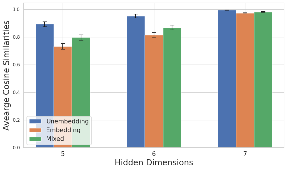
(a) $7$ Hidden Variables

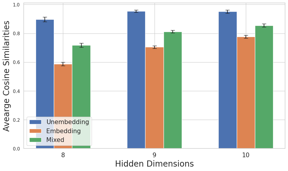
(b) $10$ Hidden Variables

Figure 6: Average cosine similarities under different hidden dimensions show that reducing dimension dose not hurt linearity significantly.

Appendix F Experiments with large language models

In this section, we will provide additional details on our experiments with LLMs.

Examples of counterfactual context and token pairs

Example context pairs from OPUS Books [Tie12] that were used to construct the embedding vectors are shown in Table 5. For the unembedding vectors, we reuse the 27 concepts considered in [PCV23] built atop the work of [GDM16], and they are listed in Table 6 along with example token pairs.

Winograd Schema

We now present full details about our experiments on the Winograd Schema dataset [LDM12]. Recall that we consider context pairs arising from the Winograd Schema, which is a dataset of pairs of sentences that differ in only one or two words and which further contain an ambiguity that can only be resolved with world knowledge and reasoning. Example context pairs from the Winograd Schema [LDM12] are shown in Table 7. Note the final 2 context pairs in the table, which have ambiguous concepts, thus highlighting the nuances of this dataset as well as of natural language. We filter the dataset to have the ambiguous word near the end of the sentence to better align with our theory.

We again compute the unembedding vectors for these context pairs output by LLaMA-2. For the embedding vectors, since there is no predefined set of concepts to consider (for instance consider the ambiguous examples), we therefore take the difference of the embedding vectors for the first token that differs in these corresponding pairs of sentences. We compute all pairwise cosine similarities. We observe that for non-matching contexts, the average similarity is 0.011 with a maximum of 0.081, whereas for matching contexts, the average similarity is 0.042 with a maximum of 0.161. This aligns with our predictions that the embedding vectors align better with the unembedding vectors of the same concept.

As an additional experiment, we compute similarities between these Winograd context pairs and the 27 concepts from [PCV23] described above. In Table 8, we display the top 3 pairs of contexts and concepts that have the highest similarities. The alignment seems reasonable as baby, woman, male, and female are different attributes of a person; and wide vs narrow and short vs tall can be construed as different manifestations of small vs big.

Table 5: Example language context pairs from OPUS Books

Language pair	Context 1	Context 2
French–Spanish	Quinze ou seize, répliqua l’autre	Quince ó diez y seis, replicó el otro
French–German	Comment est-il mon maître?	Wie ist er mein Herr?
English–French	I hesitated for a moment.	J’hésitai une seconde.
German–Spanish	Ich hasse die Spazierfahrten	No me gusta salir en coche.

Table 6: Concepts and example token pairs, taken from [PCV23]

Concept	Example token pair	Concept	Example token pair
verb $\Rightarrow$ 3pSg	(accept, accepts)	verb $\Rightarrow$ Ving	(add, adding)
verb $\Rightarrow$ Ved	(accept, accepted)	Ving $\Rightarrow$ 3pSg	(adding, adds)
Ving $\Rightarrow$ Ved	(adding, added)	3pSg $\Rightarrow$ Ved	(adds, added)
verb $\Rightarrow$ V + able	(accept, acceptable)	verb $\Rightarrow$ V + er	(begin, beginner)
verb $\Rightarrow$ V + tion	(compile, compilation)	verb $\Rightarrow$ V + ment	(agree, agreement)
adj $\Rightarrow$ un + adj	(able, unable)	adj $\Rightarrow$ adj + ly	(according, accordingly)
small $\Rightarrow$ big	(brief, long)	thing $\Rightarrow$ color	(ant, black)
thing $\Rightarrow$ part	(bus, seats)	country $\Rightarrow$ capital	(Austria, Vienna)
pronoun $\Rightarrow$ possessive	(he, his)	male $\Rightarrow$ female	(actor, actress)
lower $\Rightarrow$ upper	(always, Always)	noun $\Rightarrow$ plural	(album, albums)
adj $\Rightarrow$ comparative	(bad, worse)	adj $\Rightarrow$ superlative	(bad, worst)
frequent $\Rightarrow$ infrequent	(bad, terrible)	English $\Rightarrow$ French	(April, avril)
French $\Rightarrow$ German	(ami, Freund)	French $\Rightarrow$ Spanish	(année, año)
German $\Rightarrow$ Spanish	(Arbeit, trabajo)

Table 7: Example context pairs from Winograd Schema

Contexts

The delivery truck zoomed by the school bus because it was going so fast.

The delivery truck zoomed by the school bus because it was going so slow.

The man couldn’t lift his son because he was so weak.

The man couldn’t lift his son because he was so heavy.

Joe’s uncle can still beat him at tennis, even though he is 30 years younger.

Joe’s uncle can still beat him at tennis, even though he is 30 years older.

Paul tried to call George on the phone, but he wasn’t successful.

Paul tried to call George on the phone, but he wasn’t available.

The large ball crashed right through the table because it was made of steel.

The large ball crashed right through the table because it was made of styrofoam.

Table 8: Top similarities between Winograd contexts and token concepts

Contexts	Most similar concept	Similarity
Anne gave birth to a daughter last month. She is a very charming woman.	male$\Rightarrow$female	0.311
Anne gave birth to a daughter last month. She is a very charming baby .
The table won’t fit through the doorway because it is too wide.	small$\Rightarrow$big	0.309
The table won’t fit through the doorway because it is too narrow.
John couldn’t see the stage with Billy in front of him because he is so short.	small$\Rightarrow$big	0.303
John couldn’t see the stage with Billy in front of him because he is so tall.

Additional barplots

The entire set of similarity barplots for the concepts of French–Spanish, French–German, English–French and German–Spanish are in Figures 8, 9, 10 and 11 respectively. As we see, they satisfy the same behavior as described earlier in Section 5.2, exhibiting relatively high similarity with the matching unembedding vector, close to high similarity with related language concepts and low similarity with unrelated concepts.

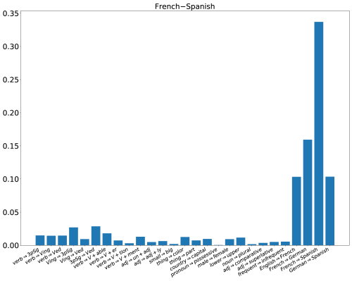
Figure 8: The French–Spanish concept is highly correlated with similar token concepts relative to others. This figure shows all cosine similarities between the French–Spanish concept and token concepts.

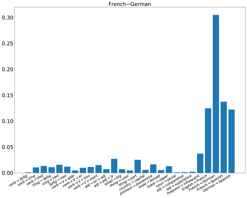
Figure 9: The French–German concept is highly correlated with similar token concepts relative to others. This figure shows all cosine similarities between the French–German concept and token concepts.

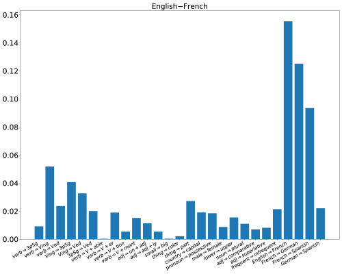
Figure 10: The English–French concept is highly correlated with similar token concepts relative to others. This figure shows all cosine similarities between the English–French concept and token concepts.

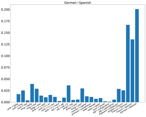
Figure 11: The German–Spanish concept is highly correlated with similar token concepts relative to others. This figure shows all cosine similarities between the German–Spanish concept and token concepts.

References

• [ABH19] Carl Allen, Ivana Balazevic and Timothy Hospedales “What the vec? towards probabilistically grounded embeddings” In Advances in neural information processing systems 32, 2019
• [AH19] Carl Allen and Timothy Hospedales “Analogies explained: Towards understanding word embeddings” In International Conference on Machine Learning, 2019, pp. 223–231 PMLR
• [Aro+13] Sanjeev Arora et al. “A Practical Algorithm for Topic Modeling with Provable Guarantees” In Proceedings of the 30th International Conference on Machine Learning, ICML 2013, Atlanta, GA, USA, 16-21 June 2013 28, JMLR Workshop and Conference Proceedings JMLR.org, 2013, pp. 280–288
• [Aro+15] Sanjeev Arora et al. “Random walks on context spaces: Towards an explanation of the mysteries of semantic word embeddings” In arXiv preprint arXiv:1502.03520, 2015, pp. 385–399
• [Aro+16] Sanjeev Arora et al. “A latent variable model approach to pmi-based word embeddings” In Transactions of the Association for Computational Linguistics 4 MIT Press One Rogers Street, Cambridge MA 02142-1209, USA journals-info …, 2016, pp. 385–399
• [Aro+18] Sanjeev Arora et al. “Linear algebraic structure of word senses, with applications to polysemy” In Transactions of the Association for Computational Linguistics 6, 2018, pp. 483–495
• [Bau+17] David Bau et al. “Network dissection: Quantifying interpretability of deep visual representations” In Proceedings of the IEEE conference on computer vision and pattern recognition, 2017, pp. 6541–6549
• [BL06] David M Blei and John D Lafferty “Dynamic topic models” In Proceedings of the 23rd international conference on Machine learning, 2006, pp. 113–120
• [Buc+23] Simon Buchholz et al. “Learning Linear Causal Representations from Interventions under General Nonlinear Mixing” In arXiv preprint arXiv:2306.02235, 2023
• [Bur+22] Collin Burns, Haotian Ye, Dan Klein and Jacob Steinhardt “Discovering latent knowledge in language models without supervision” In arXiv preprint arXiv:2212.03827, 2022
• [CTB22] Tyler A Chang, Zhuowen Tu and Benjamin K Bergen “The geometry of multilingual language model representations” In arXiv preprint arXiv:2205.10964, 2022
• [Che+21] Boli Chen et al. “Probing BERT in hyperbolic spaces” In arXiv preprint arXiv:2104.03869, 2021
• [Das99] Sanjoy Dasgupta “Learning mixtures of Gaussians” In 40th Annual Symposium on Foundations of Computer Science (Cat. No. 99CB37039), 1999, pp. 634–644 IEEE
• [Elh+22] Nelson Elhage et al. “Toy models of superposition” In arXiv preprint arXiv:2209.10652, 2022
• [EHR17] Jesse Engel, Matthew Hoffman and Adam Roberts “Latent constraints: Learning to generate conditionally from unconditional generative models” In arXiv preprint arXiv:1711.05772, 2017
• [EDH18] Kawin Ethayarajh, David Duvenaud and Graeme Hirst “Towards understanding linear word analogies” In arXiv preprint arXiv:1810.04882, 2018
• [Fal+21] Fabian Falck et al. “Multi-facet clustering variational autoencoders” In Advances in Neural Information Processing Systems 34, 2021
• [FG19] Abraham Frandsen and Rong Ge “Understanding composition of word embeddings via tensor decomposition” In arXiv preprint arXiv:1902.00613, 2019
• [GAM17] Alex Gittens, Dimitris Achlioptas and Michael W. Mahoney “Skip-Gram - Zipf + Uniform = Vector Additivity” In Annual Meeting of the Association for Computational Linguistics, 2017
• [GAM17a] Alex Gittens, Dimitris Achlioptas and Michael W Mahoney “Skip-gram- zipf+ uniform= vector additivity” In Proceedings of the 55th Annual Meeting of the Association for Computational Linguistics (Volume 1: Long Papers), 2017, pp. 69–76
• [GDM16] Anna Gladkova, Aleksandr Drozd and Satoshi Matsuoka “Analogy-based detection of morphological and semantic relations with word embeddings: what works and what doesn’t.” In Proceedings of the NAACL Student Research Workshop, 2016, pp. 8–15
• [Gur+23] Wes Gurnee et al. “Finding Neurons in a Haystack: Case Studies with Sparse Probing” In arXiv preprint arXiv:2305.01610, 2023
• [HKM23] Aapo Hyvärinen, Ilyes Khemakhem and Ricardo Monti “Identifiability of latent-variable and structural-equation models: from linear to nonlinear” In arXiv preprint arXiv:2302.02672, 2023
• [JA23] Yibo Jiang and Bryon Aragam “Learning Latent Causal Graphs with Unknown Interventions” In Advances in Neural Information Processing Systems, 2023
• [JAV23] Yibo Jiang, Bryon Aragam and Victor Veitch “Uncovering meanings of embeddings via partial orthogonality” In arXiv preprint arXiv:2310.17611, 2023
• [Khe+20] Ilyes Khemakhem, Diederik Kingma, Ricardo Monti and Aapo Hyvarinen “Variational autoencoders and nonlinear ica: A unifying framework” In International Conference on Artificial Intelligence and Statistics, 2020, pp. 2207–2217 PMLR
• [Kim+18] Been Kim et al. “Interpretability beyond feature attribution: Quantitative testing with concept activation vectors (tcav)” In International conference on machine learning, 2018, pp. 2668–2677 PMLR
• [KB15] Diederik P. Kingma and Jimmy Ba “Adam: A Method for Stochastic Optimization” In 3rd International Conference on Learning Representations, ICLR 2015, San Diego, CA, USA, May 7-9, 2015, Conference Track Proceedings, 2015
• [Kiv+21] Bohdan Kivva, Goutham Rajendran, Pradeep Ravikumar and Bryon Aragam “Learning latent causal graphs via mixture oracles” In Advances in Neural Information Processing Systems 34: Annual Conference on Neural Information Processing Systems 2021, NeurIPS 2021, December 6-14, 2021, virtual, 2021, pp. 18087–18101
• [Kiv+22] Bohdan Kivva, Goutham Rajendran, Pradeep Ravikumar and Bryon Aragam “Identifiability of deep generative models without auxiliary information” In Advances in Neural Information Processing Systems 35, 2022, pp. 15687–15701
• [KF09] Daphne Koller and Nir Friedman “Probabilistic graphical models: principles and techniques” MIT press, 2009
• [KY03] Harold Kushner and G George Yin “Stochastic approximation and recursive algorithms and applications” Springer Science & Business Media, 2003
• [Lac+22] Sébastien Lachapelle et al. “Disentanglement via Mechanism Sparsity Regularization: A New Principle for Nonlinear ICA” In 1st Conference on Causal Learning and Reasoning, CLeaR 2022, Sequoia Conference Center, Eureka, CA, USA, 11-13 April, 2022 177, Proceedings of Machine Learning Research PMLR, 2022, pp. 428–484
• [LDM12] Hector Levesque, Ernest Davis and Leora Morgenstern “The winograd schema challenge” In Thirteenth International Conference on the Principles of Knowledge Representation and Reasoning, 2012 Citeseer
• [Li+20] Bohan Li et al. “On the sentence embeddings from pre-trained language models” In arXiv preprint arXiv:2011.05864, 2020
• [Li+23] Kenneth Li et al. “Inference-Time Intervention: Eliciting Truthful Answers from a Language Model” In arXiv preprint arXiv:2306.03341, 2023
• [Lia+22] Victor Weixin Liang et al. “Mind the gap: Understanding the modality gap in multi-modal contrastive representation learning” In Advances in Neural Information Processing Systems 35, 2022, pp. 17612–17625
• [McG+22] Thomas McGrath et al. “Acquisition of chess knowledge in alphazero” In Proceedings of the National Academy of Sciences 119.47 National Acad Sciences, 2022, pp. e2206625119
• [MYZ13] Tomáš Mikolov, Wen-tau Yih and Geoffrey Zweig “Linguistic regularities in continuous space word representations” In Proceedings of the 2013 conference of the north american chapter of the association for computational linguistics: Human language technologies, 2013, pp. 746–751
• [MT17] David Mimno and Laure Thompson “The strange geometry of skip-gram with negative sampling” In Conference on Empirical Methods in Natural Language Processing, 2017
• [Mos+22] Luca Moschella et al. “Relative representations enable zero-shot latent space communication” In arXiv preprint arXiv:2209.15430, 2022
• [NLW23] Neel Nanda, Andrew Lee and Martin Wattenberg “Emergent Linear Representations in World Models of Self-Supervised Sequence Models” In arXiv preprint arXiv:2309.00941, 2023
• [Ope23] OpenAI “GPT-4 Technical Report”, 2023 arXiv:2303.08774 [cs.CL]
• [PCV23] Kiho Park, Yo Joong Choe and Victor Veitch “The Linear Representation Hypothesis and the Geometry of Large Language Models”, 2023 arXiv:2311.03658 [cs.CL]
• [Pea09] Judea Pearl “Causality” Cambridge university press, 2009
• [PSM14] Jeffrey Pennington, Richard Socher and Christopher D Manning “Glove: Global vectors for word representation” In Proceedings of the 2014 conference on empirical methods in natural language processing (EMNLP), 2014, pp. 1532–1543
• [RMC15] Alec Radford, Luke Metz and Soumith Chintala “Unsupervised representation learning with deep convolutional generative adversarial networks” In arXiv preprint arXiv:1511.06434, 2015
• [Rag+17] Maithra Raghu, Justin Gilmer, Jason Yosinski and Jascha Sohl-Dickstein “Svcca: Singular vector canonical correlation analysis for deep understanding and improvement” In stat 1050, 2017, pp. 19
• [Raj+24] Goutham Rajendran et al. “Learning Interpretable Concepts: Unifying Causal Representation Learning and Foundation Models” In arXiv preprint, 2024
• [Raj+21] Goutham Rajendran, Bohdan Kivva, Ming Gao and Bryon Aragam “Structure learning in polynomial time: Greedy algorithms, Bregman information, and exponential families” In Advances in Neural Information Processing Systems 34, 2021, pp. 18660–18672
• [Raj+23] Goutham Rajendran, Patrik Reizinger, Wieland Brendel and Pradeep Ravikumar “An Interventional Perspective on Identifiability in Gaussian LTI Systems with Independent Component Analysis” In arXiv preprint arXiv:2311.18048, 2023
• [Rei+19] Emily Reif et al. “Visualizing and measuring the geometry of BERT” In Advances in Neural Information Processing Systems 32, 2019
• [RLV23] Narutatsu Ri, Fei-Tzin Lee and Nakul Verma “Contrastive Loss is All You Need to Recover Analogies as Parallel Lines” In arXiv preprint arXiv:2306.08221, 2023
• [RB17] Maja Rudolph and David Blei “Dynamic bernoulli embeddings for language evolution” In arXiv preprint arXiv:1703.08052, 2017
• [Rud+16] Maja Rudolph, Francisco Ruiz, Stephan Mandt and David Blei “Exponential family embeddings” In Advances in Neural Information Processing Systems 29, 2016
• [SK22] Bernhard Schölkopf and Julius Kügelgen “From statistical to causal learning” In arXiv preprint arXiv:2204.00607, 2022
• [Sch+21] Bernhard Schölkopf et al. “Toward causal representation learning” arXiv:2102.11107 In Proceedings of the IEEE 109.5 IEEE, 2021, pp. 612–634
• [Sch+23] Lisa Schut et al. “Bridging the Human-AI Knowledge Gap: Concept Discovery and Transfer in AlphaZero” In arXiv preprint arXiv:2310.16410, 2023
• [Sou+18] Daniel Soudry et al. “The implicit bias of gradient descent on separable data” In The Journal of Machine Learning Research 19.1 JMLR. org, 2018, pp. 2822–2878
• [SGS00] Peter Spirtes, Clark N Glymour and Richard Scheines “Causation, prediction, and search” MIT press, 2000
• [SU22] Chandler Squires and Caroline Uhler “Causal structure learning: a combinatorial perspective” In Foundations of Computational Mathematics Springer, 2022, pp. 1–35
• [Tie12] Jörg Tiedemann “Parallel Data, Tools and Interfaces in OPUS” In Proceedings of the Eight International Conference on Language Resources and Evaluation (LREC’12) Istanbul, Turkey: European Language Resources Association (ELRA), 2012
• [Tig+23] Curt Tigges, Oskar John Hollinsworth, Atticus Geiger and Neel Nanda “Linear Representations of Sentiment in Large Language Models” In arXiv preprint arXiv:2310.15154, 2023
• [Tou+23] Hugo Touvron et al. “Llama: Open and efficient foundation language models” In arXiv preprint arXiv:2302.13971, 2023
• [Tra+23] Matthew Trager et al. “Linear spaces of meanings: compositional structures in vision-language models” In Proceedings of the IEEE/CVF International Conference on Computer Vision, 2023, pp. 15395–15404
• [Var+23] Burak Varici et al. “Score-based Causal Representation Learning with Interventions” In arXiv preprint arXiv:2301.08230, 2023
• [VM20] Riccardo Volpi and Luigi Malagò “Evaluating Natural Alpha Embeddings on Intrinsic and Extrinsic Tasks” In Workshop on Representation Learning for NLP, 2020
• [VM21] Riccardo Volpi and Luigi Malagò “Natural alpha embeddings” In Information Geometry 4.1 Springer, 2021, pp. 3–29
• [Wan+23] Zihao Wang, Lin Gui, Jeffrey Negrea and Victor Veitch “Concept Algebra for Score-based Conditional Model” In ICML 2023 Workshop on Structured Probabilistic Inference $\{$ $\backslash$&$\}$ Generative Modeling, 2023
• [Wu+20] Jingfeng Wu, Difan Zou, Vladimir Braverman and Quanquan Gu “Direction matters: On the implicit bias of stochastic gradient descent with moderate learning rate” In arXiv preprint arXiv:2011.02538, 2020
• [Zim+21] Roland S Zimmermann et al. “Contrastive learning inverts the data generating process” In International Conference on Machine Learning, 2021, pp. 12979–12990 PMLR