Quantitative estimates: How well does the discrete Fourier transform approximate the Fourier transform on $\mathbb{R}$?

Abstract

In order to compute the Fourier transform of a function $f$ on the real line numerically, one samples $f$ on a grid and then takes the discrete Fourier transform. We derive exact error estimates for this procedure in terms of the decay and smoothness of $f$. The analysis provides a new recipe of how to relate the number of samples, the sampling interval, and the grid size.

42QA38,65T05,94A12,43A15

1 Introduction

The fast Fourier transform (FFT) is widely used in the applied sciences for the numerical approximation of the Fourier transform

(1) $$\hat{f}(\xi)=\int_{-\infty}^{\infty}f(x)e^{-2\pi\mathrm{i}x\xi}\mathrm{d}x$$

from sampled values of $f$. Despite the overwhelming success of this approximation, there are surprisingly few rigorous investigations and, in our view, still substantial theoretical gaps when it comes to error estimates. As the FFT is a fast algorithm that computes the discrete Fourier transform, we are actually asking: how well does the discrete Fourier transform approximate the Fourier transform [8]?

Engineers and numerical practitioners compute the Fourier transform of a function $f$ on the real line as follows:

• Sample $f$ on an interval of length $p$ at $n$ equispaced points $hj$, for $j\in\mathbb{Z}$, $-\frac{n}{2}<j\leq\frac{n}{2}$, with step size $h$.

• It is then taken for granted that the scaled discrete Fourier transform of length $n$ provides an approximation for the values of the continuous Fourier transform of $f$ at $k/p$, i.e.,

  (2) $$\hat{f}\big{(}\tfrac{k}{p}\big{)}\approx h\sum_{-\frac{n}{2}<j\leq\frac{n}{2}}f(hj)e^{-2\pi\mathrm{i}\frac{kj}{n}}\,,\qquad k\in\mathbb{Z},\quad-\frac{n}{2}<k\leq\frac{n}{2}\,.$$

This practice is usually unquestioned and works like a charm. It is motivated by following approximations with quadrature and truncation,

(3) $$\hat{f}(\xi)=\int_{-\infty}^{\infty}f(x)e^{-2\pi\mathrm{i}\xi x}\mathrm{d}x\approx h\sum_{j\in\mathbb{Z}}f(hj)e^{-2\pi\mathrm{i}\xi hj}\approx h\sum_{-\frac{n}{2}<j\leq\frac{n}{2}}f(hj)e^{-2\pi\mathrm{i}\xi hj}\,.$$

For $\xi=\frac{k}{p}=\frac{k}{hn}$, the right-hand side is the scaled discrete Fourier transform (2). Yet one must ask what is the precise relation between the computed values $h\sum_{-\frac{n}{2}<j\leq\frac{n}{2}}f(hj)e^{-2\pi\mathrm{i}\frac{kj}{n}}$ and the samples $\hat{f}(\frac{k}{p})$ of the actual Fourier transform. Ideally one can provide reasonable error estimates for this approximation, and we formulate two questions:

• The numerical procedure depends on the number of samples $n$, the step size $h$, and the length $p$ of the sampled interval via the identity $p=hn$. How should $h,n$ and $p$ be chosen in dependence of the function class of $f$?

• What can be said about the asymptotic decay of the deviation in (2) when $n,p\rightarrow\infty$ and $h\to 0$?

State-of-the-art. To the best of our knowledge, there are surprisingly few investigations and even fewer quantitative error estimates in the literature.

The “Owner’s Manual for the Discrete Fourier Transform” [4, Section 6] contains a substantial chapter on the error of the discrete Fourier transform. There the error is quantified for rather special function classes, e.g., functions with compact support or functions on $\mathbb{R}$ with exponential decay with some type of finite order of smoothness conditions [4, Theorem 6.6] that are rarely met, see also our Section 3.5.

Epstein [8], whose title we borrowed, investigates the approximation of Fourier coefficients of periodic functions rather than the Fourier transform itself. The article [2] focuses on very narrow classes of functions, namely splines of order $k$ on equispaced nodes with compact support (called “canonical$-k$ functions”). An interesting variation was studied by Auslander and Grünbaum [1]. They consider functions $f\in L^{2}(\mathbb{R})$ and approximate averaged values of $\hat{f}$ from local averages of $f$ via the discrete Fourier transform. The resulting error estimate is not explicit enough to yield any form of asymptotics.

Since the right-hand side of (2) approximates the integral $\int_{-p/2}^{p/2}f(x)e^{-2\pi ikx/n}\mathrm{d}x$ by means of a Riemann sum or the trapezoidal rule, one should mention the recent error analyses [7, 11, 23, 25, 24] for the trapezoidal rule as relevant in this context. However, these error estimates require exponential decay and analyticity and do not even mention the Fourier transform.

In this paper we derive estimates for the error between the Fourier transform on the real line and the discrete Fourier transform for a large class of functions with polynomial or sub-exponential decay and finite smoothness. Our results confirm that, even under such very mild assumptions on the decay and smoothness, the folklore procedure works well and is successful. Our analysis also provides the new insight that the optimal spacing should depend on the decay of $f$ and $\hat{f}$. In view of (Q1), we identify an optimal relation between the step size $h$, the number of samples $n$, and the length of the sampling interval $p$ (the step size $\frac{1}{p}$ in frequency). To answer (Q2), we derive precise error estimates with explicit constants for function classes that are significantly larger than exponentially decaying, analytic functions. These error estimates are confirmed by numerical simulations utilizing the FFT which yield the precise asymptotics predicted by our theoretical estimates.

Our contribution. We proceed with a formal presentation of the numerical procedure and an explicit exposition of our results.

We first introduce the appropriate notation. For $n\in\mathbb{N}$, set

$$[n]:=\{j\in\mathbb{Z}:-\tfrac{n}{2}<j\leq\tfrac{n}{2}\}\,.$$

The discrete Fourier transform $\operatorname{\mathcal{F}}:\mathbb{C}^{n}\rightarrow\mathbb{C}^{n}$ of $y=(y_{j})_{j\in[n]}\in\mathbb{C}^{n}$ is

(4) $$\operatorname{\mathcal{F}}\!y=\bigg{(}\frac{1}{\sqrt{n}}\sum_{j\in[n]}y_{j}e^{-2\pi\mathrm{i}\frac{kj}{n}}\bigg{)}_{k\in[n]}\,.$$

Define the scaled sampling of a function $f$ with step size $h$ and length $n$ as

$$f_{h,n}:=\Big{(}\sqrt{h}f(hj)\Big{)}_{j\in[n]}\in\mathbb{C}^{n}\,.$$

Throughout the text we use the relation $p=hn$ between the interval length $p$, the step size $h$ and the number of samples $n$.

Our aim is to bound the approximation error

(5) $$E^{[n]}_{h}(f):=\biggl{(}\frac{1}{p}\sum_{k\in[n]}\Big{|}\hat{f}(\tfrac{k}{p})-h\sum_{j\in[n]}f(hj)e^{-2\pi\mathrm{i}\frac{kj}{n}}\Big{|}^{2}\bigg{)}^{1/2}=\big{\|}\hat{f}_{\frac{1}{p},n}-\operatorname{\mathcal{F}}\!f_{h,n}\big{\|}\,.$$

The normalization of $f_{h,n}$ and the factor $\frac{1}{p}$ in the definition of the error may seem artificial, but they are justified and natural in view of the time-frequency symmetry of the error

$$E^{[n]}_{h}(f)=E^{[n]}_{p^{-1}}(\bar{\hat{f}})\,.$$

See Appendix A for the proof. The symmetry between $f$ and $\hat{f}$ will also appear in the error estimates.

The following error estimate is a simple consequence of our main result for polynomial decay.

Theorem 1.1.

Let $a,b>1$. If $f$ and $\hat{f}$ are continuous and satisfy polynomial decay of the form $|f(x)|\lesssim(1+|x|)^{-a}$ and $|\hat{f}(\xi)|\lesssim(1+|\xi|)^{-b}$, then for all $\alpha<a-\frac{1}{2}$, $\beta<b-\frac{1}{2}$

$$E^{[n]}_{h}(f)\lesssim p^{-\alpha}\sup_{x\in\mathbb{R}}|f(x)|(1+|x|)^{a}+h^{\beta}\sup_{\xi\in\mathbb{R}}|\hat{f}(\xi)|(1+|\xi|)^{b}\,,$$

where the constants in $\lesssim$ are independent of $h$, $n$, $p$.

The error bound is balanced if $p^{-\alpha}\asymp h^{\beta}\asymp n^{-\frac{\alpha\beta}{\alpha+\beta}}$, and for this choice $E^{[n]}_{h}(f)\lesssim n^{-\frac{\alpha\beta}{\alpha+\beta}}$. This is the optimal choice for the relation between $h$, $p$, and $n$, see Corollary 3.9. Our numerical simulations in Section 2 using the FFT suggest that the bounds in Theorem 1.1 are sharp.

For the approximation procedure to make sense, we need the Fourier transform to be defined pointwise and continuous, so that $f\in L^{1}(\mathbb{R})$ is a reasonable minimal assumption. One may argue that we also make certain assumptions on $\hat{f}$, which is the very object we want to compute. If one does not like the polynomial decay condition of $\hat{f}$ in Theorem 1.1, one can replace it by a stronger condition on smoothness of $f$. Precisely, if the derivatives $f^{(l)}$ are in $L^{1}(\mathbb{R})$ for $l=0,\dots,b$ with $b\in\mathbb{N}$, then it follows that $|\hat{f}(\xi)|\lesssim(1+|\xi|)^{-b}$.

Sub-exponential decay in time and in frequency occurs importantly in the theory of test functions and distributions (under the name of Gelfand-Shilov spaces or ultra test functions) [3]. In that case, we offer the following version.

Theorem 1.2 (sub-exponential decay).

Let $r,s>0$ and $0<\alpha,\beta\leq 1$. If $f$ and $\hat{f}$ are continuous and satisfy the decay conditions $|f(x)|\lesssim e^{-r|x|^{\alpha}}$ and $|\hat{f}(\xi)|\lesssim e^{-s|x|^{\beta}}$, then for all $r^{\prime}<r$,$s^{\prime}<s$,

$$E^{[n]}_{h}(f)\lesssim e^{-r^{\prime}(\frac{p}{2})^{\alpha}}\sup_{x\in\mathbb{R}}|f(x)|e^{r|x|^{\alpha}}+e^{-s^{\prime}(2h)^{-\beta}}\sup_{\xi\in\mathbb{R}}|\hat{f}(\xi)|e^{s|\xi|^{\beta}}\,.$$

For $r^{\prime}\to r$ and $s^{\prime}\to s$ the error is balanced if $e^{-r(\frac{p}{2})^{\alpha}}\asymp e^{-s(2h)^{-\beta}}$, which is satisfied for $h=n^{-\frac{\alpha}{\alpha+\beta}}\left(\tfrac{s}{r}\right)^{\frac{1}{\alpha+\beta}}2^{\frac{\alpha-\beta}{\alpha+\beta}}$. This condition on $h$ is the optimal choice for the relation between $h$, $p,$ and $n$, see Corollary 3.15.

We also provide bounds for mixed decay.

Theorem 1.3 (mixed decay).

Let $r>0$ and $0<\alpha\leq 1$. If $f$ and $\hat{f}$ are continuous and satisfy $|f(x)|\lesssim e^{-r|x|^{\alpha}}$ and $|\hat{f}(\xi)|\lesssim(1+|\xi|)^{-b}$ with $b>1$, then, for all $r^{\prime}<r$ and $\beta<b-\frac{1}{2}$,

(6) $$E^{[n]}_{h}(f)\lesssim e^{-r^{\prime}(\frac{p}{2})^{\alpha}}\sup_{x\in\mathbb{R}}|f(x)|e^{r|x|}+h^{\beta}\sup_{\xi\in\mathbb{R}}|\hat{f}(\xi)|(1+|\xi|)^{b}\,.$$

For all practical purposes, the length of the sampled interval $p$ is sufficiently large, so that $e^{-r^{\prime}(\frac{p}{2})^{\alpha}}$ is negligible (and may for instance even be close to machine precision). Then the error is dominated by the polynomial term $h^{\beta}$.

In the main theoretical part in Section 3, we will derive more general results by quantifying the decay of a function by means of its membership in a Wiener amalgam space. This is the canonical function class when sampling is involved [9, 10, 12].

Software to plot the discrete Fourier transform commonly performs interpolation of the computed data vector $\operatorname{\mathcal{F}}\!f_{h,n}$. In order to simulate this process, we use three representative interpolation procedures and derive bounds on their deviation from $\hat{f}$ on the real line. One of them is based on the cardinal sine function $\operatorname*{sinc}(x)=\frac{\sin(\pi x)}{\pi x}$ that is widely used in digital signal processing. The computation of $\operatorname{\mathcal{F}}\!f_{h,n}$ gives rise to the approximation of $\hat{f}$ on the real line by

$$\hat{f}(\xi)\approx\sqrt{p}\sum_{k\in[n]}(\mathcal{F}f_{h,n})(k)\operatorname*{sinc}(p\xi-k)=h\sum_{k,j\in[n]}f(hj)e^{-2\pi\mathrm{i}\frac{kj}{n}}\operatorname*{sinc}(p\xi-k)\,.$$

So the error is then $\|\hat{f}-h\sum_{k,j\in[n]}f(hj)e^{-2\pi\mathrm{i}\frac{kj}{n}}\operatorname*{sinc}(p\cdot-k)\|_{L^{2}(\mathbb{R})}$. We will show in Section 5, Theorem 4.1, that this error obeys the same bounds as in Theorems 1.1, 1.2, and 1.3. The proof uses the estimates for $E^{[n]}_{h}(f)$.

Outline: Section 2 is dedicated to numerical experiments using the FFT and fully supports the theoretical results of Theorems 1.1 and 1.3. The full versions of the theoretical results on the approximation rates for spaces of polynomial and sub-exponential decay in time and in frequency are derived in Section 3. The approximation of $\hat{f}$ on the real line is discussed in Section 4. We investigate minimal requirements on $f$ and $\hat{f}$ for convergence in Section 5.

2 Numerical experiments for polynomial decay

Since our priority is the practical impact of the error estimates, we first offer numerical evidence that the error bounds of Theorem 1.1 are sharp for polynomial weights.

2.1 Polynomial decay in time and in frequency

In view of Theorem 1.1, we construct a family $f^{a,b}$ of functions with exact polynomial decay $a$ in time and $b$ in frequency such that each function and its Fourier transform can be numerically evaluated with sufficient accuracy.

We use linear combinations of shifts of the cardinal B-splines defined by $B_{1}:={\bf 1}_{[-\frac{1}{2},\frac{1}{2})}$, and

$$B_{b+1}:=B_{b}*B_{1},\qquad b=1,2,\ldots\,.$$

Each $B_{b}$ is a piecewise polynomial function of degree $b-1$ that is $b-2$-times continuously differentiable with support $[-\frac{b}{2},\frac{b}{2}]$, see [20] and also [19, Section 9.1].

Consider $(c_{k})_{k\in\mathbb{Z}}\subseteq\mathbb{C}$ given by its nonzero entries

$$c_{0}=\frac{1}{2},\qquad c_{k}=\frac{1}{k\pi\mathrm{i}},\text{ for }k\in 2\mathbb{Z}+1\,,$$

so that $c_{2k}=0$. We study the family of functions

(7) $$f^{a,b}(x):=\sum_{k\in\mathbb{Z}}c^{a}_{k}\,B_{b}(x-k),\qquad a,b=1,2,\ldots\,,$$

which consists of locally finite sums. Therefore the point evaluations can be evaluated accurately in numerical experiments, and they satisfy $|f^{a,b}(x)|\lesssim(1+|x|)^{-a}$.

To compute the Fourier transform of $f^{a,b}$, we define the Fourier series $u_{a}(\xi):=\sum_{k\in\mathbb{Z}}c^{a}_{k}e^{-2\pi\mathrm{i}k\xi}$. As $\widehat{B_{b}}=\operatorname*{sinc}^{b}$, we observe

$$\widehat{f^{a,b}}(\xi) =\operatorname*{sinc}(\xi)^{b}\sum_{k\in\mathbb{Z}}c^{a}_{k}e^{-2\pi\mathrm{i}k\xi}=\operatorname*{sinc}(\xi)^{b}u_{a}(\xi)\,.$$

The estimate $|\operatorname*{sinc}^{b}(\xi)|\lesssim(1+|\xi|)^{-b}$ implies $|\widehat{f^{a,b}}(\xi)|\lesssim(1+|\xi|)^{-b}$, thus $f^{a,b}$ satisfies the assumptions of Theorem 1.1.

By a short computation we find $u_{1}(\xi)={\bf 1}_{(-\frac{1}{2},0)}(\xi)+\frac{1}{2}{\bf 1}_{\{-\frac{1}{2},0\}}(\xi)$ for $\xi\in[-\frac{1}{2},\frac{1}{2})$, and then $u_{a+1}$ is the cyclic convolution of $u_{a}$ and $u_{1}$, i.e.,

$$u_{a+1}(\xi)=\int_{\mathbb{R}/\mathbb{Z}}u_{a}(\eta)u_{1}(\xi-\eta)\mathrm{d}\eta,\qquad a=1,2,\ldots\,.$$

For $a=2,3$ we have $u_{2}(\xi)=|\xi|$ $u_{a}$ for $\xi\in[-\frac{1}{2},\frac{1}{2})$, and $u_{3}(\xi)=\operatorname*{sign}(\xi)\xi^{2}-\frac{1}{2}\xi+\frac{1}{8}$. Thus, we can evaluate the point evaluations of $f^{a,b}$ and $\widehat{f^{a,b}}$ exactly, both analytically and numerically, and the decay is labeled by $a$ and $b$. For the numerical simulations we compute the samples $\widehat{f^{a,b}}(k/p)$ and compare them with the discrete Fourier transform of a sampled version of $f^{a,b}$.

Since the error estimates of Theorem 1.1 work for every parameter $\alpha<a-1/2$ and $\beta<b-1/2$, we will plot the error curves with the values $\alpha=a-\frac{1}{2}$ and $\beta=b-\frac{1}{2}$ and compare our numerical observations with the error rate $n^{-\frac{\alpha\beta}{\alpha+\beta}}$ for $h=n^{-\frac{\alpha}{\alpha+\beta}}$. The infinitesimal difference between $\alpha<a-1/2$ and $\alpha=a-1/2$ is not visible.

To compute the discrete Fourier transform, we choose $n=2^{l}$, $l=10,\ldots,20$ in Theorem 1.1 and then apply the FFT to the samples $f^{a,b}_{h,n}$. The FFT is taken from the Julia package FFTW.jl with $64$-bit floating point arithmetics. The package provides a binding to the C library FFTW [13].

The approximation rates, predicted by Theorem 1.1, are $n^{-\frac{\alpha\beta}{\alpha+\beta}}\asymp h^{\beta}$, see Table 1 for some combinations of $a$ and $b$. To stick to $L^{1}(\mathbb{R})$ functions, we skip $a=1$.

$a$	$b$	$\alpha=a-\frac{1}{2}$	$\beta=b-\frac{1}{2}$	$h=n^{-\frac{\alpha}{\alpha+\beta}}$	$p=nh=n^{\frac{\beta}{\alpha+\beta}}$	$E^{[n]}_{h}(f^{a,b})\asymp h^{\beta}=n^{-\frac{\alpha\beta}{\alpha+\beta}}$
$2$	$2$	$3/2$	$3/2$	$n^{-1/2}$	$n^{1/2}$	$n^{-3/4}$
$2$	$3$	$3/2$	$5/2$	$n^{-3/8}$	$n^{5/8}$	$n^{-15/16}$
$2$	$4$	$3/2$	$7/2$	$n^{-3/10}$	$n^{7/10}$	$n^{-21/20}$
$3$	$2$	$5/2$	$3/2$	$n^{-5/8}$	$n^{3/8}$	$n^{-15/16}$
$3$	$3$	$5/2$	$5/2$	$n^{-1/2}$	$n^{1/2}$	$n^{-5/4}$
$3$	$4$	$5/2$	$7/2$	$n^{-5/12}$	$n^{7/12}$	$n^{-35/24}$

Table 1: List of the relevant values of Theorem 1.1 for $f^{a,b}$, so that $E^{[n]}_{h}(f^{a,b})$ is bounded by $h^{\beta}=p^{-\alpha}=n^{-\frac{\alpha\beta}{\alpha+\beta}}$.

Our numerical experiments as illustrated in Figure 1 align with the theoretical bounds in Theorem 1.1 and suggest that they are sharp.

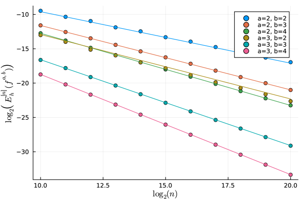
Figure 1: Logarithmic plots of $E^{[n]}_{h}(f^{a,b})$ for various $a$ and $b$. Points are computed numerically for $n=2^{l}$, $l=10,\ldots,20$. Reference lines represent the theoretical slopes from Theorem 1.1 listed in Table 1.

Remark 2.1.

The closed form expressions for $u_{a}(\xi)=\sum_{k\in\mathbb{Z}}c^{a}_{k}e^{-2\pi\mathrm{i}k\xi}$ are key to our numerical results: Without a closed form expression of $u_{a}$ the series in (7) would need to be truncated for evaluation. The truncation error is accompanied by competing floating point errors due to the summation. We found it difficult to identify a sufficiently accurate truncation that yields reliable numerical estimates for $E^{[n]}_{h}(f^{a,b})$.

2.2 Polynomial decay in frequency

To test Theorem 1.3, we consider $f(x)=e^{-2\pi|x|}$. Its Fourier transform is $\hat{f}(\xi)=\frac{1}{\pi(1+\xi^{2})}$, so that $r=2\pi$, $\alpha=1$, and $|\widehat{f}(\xi)|\lesssim(1+|\xi|)^{-b}$ with $b=2$.

For increasing values of $n$ in numerical experiments with the FFT, we choose successively $p=n^{1/2}$, $p=6n^{1/10}$, and $p=10$, so that $h=n^{-1/2}$, $h=6n^{-9/10}$, and $h=10n^{-1}$, respectively. Note that $p$ is sufficiently large, so that the error bound in Theorem 1.3 is expected to be governed by the polynomial term for a large range of $n$. Hence, we expect to observe the decay rate $h^{\frac{3}{2}}$, which is $n^{-\frac{3}{4}}$, $n^{-\frac{27}{10}}$, and $n^{-\frac{3}{2}}$, respectively. Figure 2 shows the results of our numerical experiments. Again, they match the theoretical prediction perfectly.

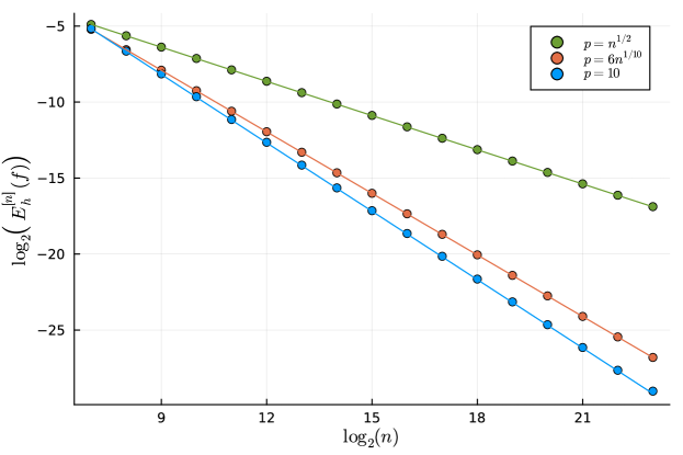
Figure 2: Logarithmic plots of $E^{[n]}_{h}(f)$ for $f(x)=e^{-2\pi|x|}$. Points are computed numerically for $n=2^{l}$, $l=7,\ldots,23$. We choose $p=n^{\frac{1}{2}}$, $p=6n^{1/10}$, and $p=10$. Reference lines represent the theoretical slope $h^{\beta}$ with $\beta=\frac{3}{2}$ that leads to $n^{-\frac{3}{4}}$, $n^{-\frac{27}{20}}$, and $n^{-\frac{3}{2}}$, respectively. Points align well with theoretical predictions.

3 Approximation rates

In this section we derive general and explicit bounds on the approximation error $E^{[n]}_{h}(f)=\|\hat{f}_{\frac{1}{p},n}-\operatorname{\mathcal{F}}\!f_{h,n}\|$ in (5) by decomposing the error into a time and a frequency component that are estimated separately. These components arise from approximating $\hat{f}(\tfrac{k}{p})$ first by a Riemannian sum and then truncating it as in (3),

(8) $$\hat{f}\big{(}\tfrac{k}{p}\big{)}\approx h\sum_{j\in\mathbb{Z}}f(hj)e^{-2\pi\mathrm{i}\frac{k}{p}hj}\approx h\sum_{j\in[n]}f(hj)e^{-2\pi\mathrm{i}\frac{kj}{n}}=\sqrt{hn}(\operatorname{\mathcal{F}}\!f_{h,n})(k)\,.$$

The left-hand side is the sampled (continuous) Fourier transform, the right-hand side is its approximation by the discrete Fourier transform. The idea is to estimate the discretization error $\hat{f}\big{(}\tfrac{k}{p}\big{)}-h\sum_{j\in\mathbb{Z}}f(hj)e^{-2\pi\mathrm{i}\frac{k}{p}hj}$ by the decay of $\hat{f}$, and the truncation $h\sum_{j\in\mathbb{Z}\setminus[n]}f(hj)e^{-2\pi\mathrm{i}\frac{k}{p}hj}$ by the decay of $f$.

3.1 Error decomposition into time and frequency components

The continuous functions on the real line are denoted by $\mathcal{C}=\mathcal{C}(\mathbb{R})$. We consider the Wiener amalgam space $W(\mathcal{C},\ell^{1})$ that consists of all continuous functions $f$ such that

(9) $$\|f\|_{W(\mathcal{C},\ell^{1})}:=\sum_{l\in\mathbb{Z}}\sup_{x\in[0,1]}\left|f(x+l)\right|$$

is finite, cf. [9, 10, 12]. If $f\in W(\mathcal{C},\ell^{1})$, then the sampling operator $f\mapsto(f(hj))_{j\in\mathbb{Z}}\in\ell^{1}(\mathbb{Z})$ is bounded for all $h>0$, and consequently the $p$-periodization

$$\mathcal{P}\!_{p}f(x)=\sum_{l\in\mathbb{Z}}f(x+pl)$$

converges absolutely and uniformly for every $p>0$. For $f,\hat{f}\in W(\mathcal{C},\ell^{1})$, the Poisson summation formula $\sum_{l\in\mathbb{Z}}f(x+pl)=\frac{1}{p}\sum_{k\in\mathbb{Z}}\hat{f}(\tfrac{k}{p})e^{2\pi i\frac{k}{p}x}$ holds pointwise for all $x\in\mathbb{R}$, cf. [14, Lemma 4].

The following identity provides the foundation of our approach and will facilitate the error decomposition in a time and a frequency component.

Lemma 3.1.

If $f,\hat{f}\in W(\mathcal{C},\ell^{1})$, then, for $k\in[n]$,

(10) $$h\sum_{j\in\mathbb{Z}}f(hj)e^{-2\pi\mathrm{i}\frac{k}{p}hj}=h\sum_{j\in[n]}(\mathcal{P}\!_{p}f)(hj)e^{-2\pi\mathrm{i}\frac{kj}{n}}=(\mathcal{P}\!_{h^{-1}}\hat{f})(\tfrac{k}{p})\,.$$

We may also write the second identity in terms of $(\mathcal{P}\!_{h^{-1}}\hat{f})_{\frac{1}{p},n}=\mathcal{F}(\mathcal{P}\!_{p}f)_{h,n}$.

Proof 3.2.

The first identity is the Poisson summation formula applied to the $h^{-1}$-periodization of $\hat{f}$. For the second identity, we partition $\mathbb{Z}$ into residue classes modulo $n$ and use $p=hn$. Then

$$h\sum_{j\in\mathbb{Z}}f(hj)e^{-2\pi\mathrm{i}\frac{k}{p}hj} =h\sum_{j\in[n]}\sum_{l\in\mathbb{Z}}f(hj+hnl)e^{-2\pi\mathrm{i}\frac{k}{hn}(hj+hnl)}$$

$$=h\sum_{j\in[n]}\sum_{l\in\mathbb{Z}}f(hj+pl)e^{-2\pi\mathrm{i}\frac{k}{hn}hj}$$

$$=h\sum_{j\in[n]}\mathcal{P}\!_{p}f(hj)e^{-2\pi\mathrm{i}\frac{k}{n}j}\,.$$

Lemma 3.1 enables a reinterpretation of the two step approximation strategy via quadrature and truncation (8). The quadrature step compares the samples of the Fourier transform $\hat{f}(\frac{k}{p})$ to samples of the periodization of the Fourier transform $(\mathcal{P}\!_{h^{-1}}\hat{f})(\frac{k}{p})$, which coincide with the discrete Fourier transform of samples of the periodization of $f$, i.e., $\mathcal{F}(\mathcal{P}\!_{p}f)_{h,n}(k)$. The truncation compares the latter with the discrete Fourier transform $\operatorname{\mathcal{F}}\!f_{h,n}$. Symbolically,

(11) $$\hat{f}_{\frac{1}{p},n}\approx(\mathcal{P}\!_{h^{-1}}\hat{f})_{\frac{1}{p},n}=\mathcal{F}(\mathcal{P}\!_{p}f)_{h,n}\approx\operatorname{\mathcal{F}}\!f_{h,n}\,.$$

More precisely, we split the pointwise error in two components,

(12) $$|\frac{1}{\sqrt{p}}\hat{f}(\tfrac{k}{p})-\operatorname{\mathcal{F}}\!f_{h,n}(k)|\leq\frac{1}{\sqrt{p}}|\hat{f}(\tfrac{k}{p})-\mathcal{P}\!_{h^{-1}}\hat{f}(\tfrac{k}{p})|+|\operatorname{\mathcal{F}}\Big{(}(\mathcal{P}\!_{p}f-f)_{h,n}\Big{)}(k)|\,.$$

Taking norms and using the unitarity of $\operatorname{\mathcal{F}}$ we arrive at

(13) $$\begin{split}E^{[n]}_{h}(f)=\|\hat{f}_{\frac{1}{p},n}-\operatorname{\mathcal{F}}\!f_{h,n}\|\leq&\,\|(\hat{f}-\mathcal{P}\!_{h^{-1}}\hat{f})_{\frac{1}{p},n}\|+\|\operatorname{\mathcal{F}}\Big{(}(\mathcal{P}\!_{p}f-f)_{h,n}\Big{)}\|\\ =&\,\|(\hat{f}-\mathcal{P}\!_{h^{-1}}\hat{f})_{\frac{1}{p},n}\|+\|(\mathcal{P}\!_{p}f-f)_{h,n}\|\,.\end{split}$$

On the right hand side of this inequality we have (i) eliminated $\operatorname{\mathcal{F}}$ and (ii) split the error in a time component and a frequency component. Note that the symmetry of this decomposition matches the symmetry of the error $E^{[n]}_{h}(f)=E^{[n]}_{p^{-1}}(\bar{\hat{f}})$, cf. Appendix A. To derive approximation rates, we must ensure that the samples of $f-\mathcal{P}\!_{p}f$ and $\hat{f}-\mathcal{P}\!_{h^{-1}}\hat{f}$ decay sufficiently fast. This can be accomplished by specifying decay conditions on $f$ and $\hat{f}$.

3.2 General weights

We quantify the decay of a function by the use of a weight function $v:\mathbb{R}\rightarrow(0,\infty)$. We consider weights $v$ that satisfy

(14a) $$v\text{ is even: }v(-x)=v(x)\,,$$

(14b) $$v\text{ is nondecreasing, i.e., }v(x)\leq v(y),\text{ for }|x|\leq|y|\,,$$

(14c) $$v\text{ is submultiplicative, i.e., }v(x+y)\leq v(x)v(y)\text{ for }x,y\in\mathbb{R}\,,$$

(14d) $$v\text{ is inverse square-summable, }\sum_{l\in\mathbb{Z}}{|v(l)|^{-2}}<\infty\,.$$

The standard examples of weights that satisfy conditions (14a) to (14d) are the polynomial weights $v_{\alpha}=(1+|x|)^{\alpha}$ for $\alpha>\frac{1}{2}$, and the (sub-)exponential weights $v_{r,\alpha}=e^{r|x|^{\alpha}}$, for $0<\alpha\leq 1$ and $r>0$.

Associated to $v$ are the weighted sequence spaces

$$\ell^{q}_{v}:=\ell^{q}_{v}(\mathbb{Z}):=\{(c_{l})_{l\in\mathbb{Z}}\subseteq\mathbb{C}:\sum_{l\in\mathbb{Z}}|c_{l}|^{q}|v(l)|^{q}<\infty\}\,,$$

and the weighted Lebesgue space $L^{2}_{v}:=L^{2}_{v}(\mathbb{R})$ of all functions $f$ such that $\|f\|_{L^{2}_{v}}=\|fv\|_{L^{2}}$ is finite. For a constant weight $v\equiv 1$ we omit the subscript and write $\ell^{p}$ and $L^{p}$.

The Wiener amalgam space $W(\mathcal{C},\ell^{q}_{v})$ consists of all continuous functions $f$ such that

(15) $$\|f\|_{W(\mathcal{C},\ell^{q}_{v})}:=\bigg{(}\sum_{l\in\mathbb{Z}}\sup_{x\in[0,1]}\left|f(x+l)\right|^{q}|v(l)|^{q}\bigg{)}^{1/q}$$

is finite, cf. [9, 10, 12].

If $v$ satisfies (14d) then $\ell^{2}_{v}\subseteq\ell^{1}$, and we derive the continuous embeddings $W(\mathcal{C},\ell^{2}_{v})\subseteq W(\mathcal{C},\ell^{1})\subseteq L^{1}(\mathbb{R})$.

In order to bound the right hand side of the error functional $E^{[n]}_{h}(f)$ in (13), we need to estimate the deviation of $f$ and $\hat{f}$ from their respective periodizations. We derive such bounds in terms of the function

(16) $$\Phi_{v}(p):=\bigg{(}2\sum_{m=0}^{\infty}|v(pm+\tfrac{p}{2})|^{-2}\bigg{)}^{1/2}\,.$$

Observe that $\lim_{p\to\infty}\Phi_{v}(p)=0$ always holds for a weight $v$ satisfying (14). For polynomial and sub-exponential weights we obtain quantitative bounds on the decay of $\Phi_{v}(p)$ in Lemma 3.7 and in Lemma 3.13.

Lemma 3.3.

If $f\in W(\mathcal{C},\ell^{2}_{v})$, and $v$ satisfies (14) then

(i) $$\|f-\mathcal{P}\!_{p}f\|_{L^{2}(-\frac{p}{2},\frac{p}{2})} \leq v(1)\Phi_{v}(p)\|f\|_{W(\mathcal{C},\ell^{2}_{v})},$$

(ii) $$\|(f-\mathcal{P}\!_{p}f)_{h,n}\| \leq v(1)\Phi_{v}(p)(1+h)^{\frac{1}{2}}\|f\|_{W(\mathcal{C},\ell^{2}_{v})}\,.$$

Part (i) is used only in Section 4 on interpolation, but Part (ii) is crucial for bounds on $E^{[n]}_{h}$.

Proof 3.4.

(i) We bound $(f-\mathcal{P}\!_{p}f)(x)$ by the Cauchy-Schwartz inequality,

(17) $$\bigg{|}\sum_{0\neq l\in\mathbb{Z}}f(x+pl)\bigg{|}^{2}\leq\sum_{0\neq m\in\mathbb{Z}}|v(x+pm)|^{-2}\sum_{0\neq l\in\mathbb{Z}}\left|f(x+pl)\right|^{2}|v(x+pl)|^{2}\,.$$

Since $v$ is even (14a) and nondecreasing (14b), for $|x|\leq\frac{p}{2}$, the first sum can be majorized by

(18) $$\begin{split}\sum_{0\neq m\in\mathbb{Z}}|v(x+pm)|^{-2}&\leq\sum_{0\neq m\in\mathbb{Z}}|v(p|m|-\tfrac{p}{2})|^{-2}\\ &\leq 2\sum_{m=1}^{\infty}|v(pm-\tfrac{p}{2})|^{-2}=|\Phi_{v}(p)|^{2}\,.\end{split}$$

Integration of (17) yields

$$\int_{-\frac{p}{2}}^{\frac{p}{2}}\bigg{|}\sum_{0\neq l\in\mathbb{Z}}f(x+pl)\bigg{|}^{2}\mathrm{d}x \leq|\Phi_{v}(p)|^{2}\int_{-\frac{p}{2}}^{\frac{p}{2}}\sum_{0\neq l\in\mathbb{Z}}\left|f(x+pl)\right|^{2}|v(x+pl)|^{2}\mathrm{d}x$$

$$=|\Phi_{v}(p)|^{2}\int_{|x|>\frac{p}{2}}\left|f(x)\right|^{2}|v(x)|^{2}\mathrm{d}x$$

$$\leq|\Phi_{v}(p)|^{2}\|f\|^{2}_{L^{2}_{v}}\,.$$

Direct computations lead to $\|f\|_{L^{2}_{v}}\leq v(1)\|f\|_{W(\mathcal{C},\ell^{2}_{v})}$.

(ii) We use (17) and (18) for $x=hj$ and sum over $j\in[n]$, so that $p=nh$ yields

$$\sum_{j\in[n]}\bigg{(}\sum_{0\neq l\in\mathbb{Z}}\left|f(hj+pl)\right|\bigg{)}^{2} \leq|\Phi_{v}(p)|^{2}\sum_{j\in[n]}\sum_{0\neq l\in\mathbb{Z}}\left|f(hj+pl)\right|^{2}|v(hj+pl)|^{2}$$

$$=|\Phi_{v}(p)|^{2}\sum_{j\in\mathbb{Z}\setminus[n]}\left|f(hj)\right|^{2}|v(hj)|^{2}$$

$$\leq|\Phi_{v}(p)|^{2}\sum_{j\in\mathbb{Z}}\left|f(hj)\right|^{2}|v(hj)|^{2}\,.$$

Since $v$ satisfies (14a) – (14c), we derive 

$$\sum_{j\in\mathbb{Z}}\left|f(hj)\right|^{2}|v(hj)|^{2} \leq\lceil h^{-1}\rceil\sum_{l\in\mathbb{Z}}\sup_{x\in[l,l+1]}\left|f(x)\right|^{2}|v(|l|+1)|^{2}$$

$$\leq\lceil h^{-1}\rceil|v(1)|^{2}\sum_{l\in\mathbb{Z}}\sup_{x\in[0,1]}\left|f(x+l)\right|^{2}|v(l)|^{2}\,.$$

The observation $h\lceil h^{-1}\rceil\leq(1+h)$ concludes the proof.

After these preparations we can now formulate our main result. This is an error estimate for the approximation of the Fourier transform by the discrete Fourier transform with very general conditions on the decay of the function and its Fourier transform.

Theorem 3.5.

Let $f\in W(\mathcal{C},\ell^{2}_{v})$ and $\hat{f}\in W(\mathcal{C},\ell^{2}_{w})$. If the weights $v,w$ satisfy (14), then

(19) $$E^{[n]}_{h}(f)\leq v(1)\Phi_{v}(p)(1+h)^{\frac{1}{2}}\|f\|_{W(\mathcal{C},\ell^{2}_{v})}+w(1)\Phi_{w}(h^{-1})(1+\tfrac{1}{p})^{\frac{1}{2}}\|\hat{f}\|_{W(\mathcal{C},\ell^{2}_{w})}\,.$$

Note that for $0<h\leq 1\leq p$ the first term does not depend on $h$ and the second term not on $p$. Therefore

(20) $$E^{[n]}_{h}(f)\leq 2^{\frac{1}{2}}v(1)\Phi_{v}(p)\|f\|_{W(\mathcal{C},\ell^{2}_{v})}+2^{\frac{1}{2}}w(1)\Phi_{w}(h^{-1})\|\hat{f}\|_{W(\mathcal{C},\ell^{2}_{w})}\,.$$

We now prove Theorem 3.5.

Proof 3.6.

We apply Lemma 3.3 (ii) to both $f$ and $\hat{f}$. Recall the bound $E^{[n]}_{h}(f)\leq\|(\hat{f}-\mathcal{P}\!_{h^{-1}}\hat{f})_{\frac{1}{p},n}\|+\|(f-\mathcal{P}\!_{p}f)_{h,n}\|$ in (13). Lemma 3.3 estimates $\|(f-\mathcal{P}\!_{p}f)_{h,n}\|$ and yields the first term of the error in (19). Applying Lemma 3.3 to $\|(\hat{f}-\mathcal{P}\!_{h^{-1}}\hat{f})_{\frac{1}{p},n}\|$ by interchanging the roles of $f$, $p$, and $h$ with $\hat{f}$, $h^{-1}$, and $p^{-1}$, yields the second term. This concludes the proof.

Theorem 3.5 asserts a bound on the error $E^{[n]}_{h}(f)$ in terms of $\Phi_{v}(p)$ and $\Phi_{w}(h^{-1})$. For polynomial and sub-exponential weights the error estimates can be made much more explicit.

3.3 Polynomial weights

In this section we consider the polynomial weights $v_{\alpha}(x)=(1+|x|)^{\alpha}$. To bound $\Phi_{v_{\alpha}}(p)$ in (16), we make use of the Hurwitz zeta function $\zeta(s,t)=\sum_{m=0}^{\infty}(m+t)^{-s}$.

Lemma 3.7.

If $\alpha>\frac{1}{2}$, then

$$\Phi_{v_{\alpha}}(p)\leq p^{-\alpha}\sqrt{2\zeta(2\alpha,\tfrac{1}{2})}\leq p^{-\alpha}2^{\alpha+1/2}\Big{(}1+\frac{1}{4\alpha-2}\Big{)}^{1/2}\lesssim p^{-\alpha}\,.$$

Proof 3.8.

We factor out $p$ to obtain

$$|\Phi_{v_{\alpha}}(p)|^{2} =2\sum_{m=0}^{\infty}\left(1+\left|pm+\tfrac{p}{2}\right|\right)^{-2\alpha}\leq p^{-2\alpha}2\sum_{m=0}^{\infty}\left(\tfrac{1}{p}+m+\tfrac{1}{2}\right)^{-2\alpha}$$

$$\leq p^{-2\alpha}2\sum_{m=0}^{\infty}\left(m+\tfrac{1}{2}\right)^{-2\alpha}=p^{-2\alpha}2\zeta(2\alpha,\tfrac{1}{2})\,.$$

The integral test for convergence of series provides, for $\alpha>1/2$,

$$\zeta(2\alpha,\tfrac{1}{2})\leq 2^{2\alpha}+\int_{0}^{\infty}(x+\tfrac{1}{2})^{-2\alpha}\mathrm{d}x=2^{2\alpha}(1+\tfrac{1}{4\alpha-2})\,.$$

For polynomial weights Theorem 3.5 takes the following shape.

Corollary 3.9 (polynomial weights).

Assume that $f\in W(\mathcal{C},\ell^{2}_{v_{\alpha}})$ and $\hat{f}\in W(\mathcal{C},\ell^{2}_{v_{\beta}})$ for $\alpha,\beta>\frac{1}{2}$, and $0<h\leq 1\leq p$.

• Set $c_{s}=2^{2s+1}\left(1+\tfrac{1}{4s-2}\right)^{\frac{1}{2}}$. Then

  $$E^{[n]}_{h}(f)\leq c_{\alpha}p^{-\alpha}\|f\|_{W(\mathcal{C},\ell^{2}_{v_{\alpha}})}+c_{\beta}h^{\beta}\|\hat{f}\|_{W(\mathcal{C},\ell^{2}_{v_{\beta}})}\,.$$

• If the step size satisfies $h\asymp n^{-\frac{\alpha}{\alpha+\beta}}$, then

  $$E^{[n]}_{h}(f)\lesssim h^{\beta}\big{(}\|f\|_{W(\mathcal{C},\ell^{2}_{v_{\alpha}})}+\|\hat{f}\|_{W(\mathcal{C},\ell^{2}_{v_{\beta}})}\big{)}\,.$$

  Expressed with the number of samples, the error is $E^{[n]}_{h}(f)\lesssim n^{-\frac{\alpha\beta}{\alpha+\beta}}$.

Proof 3.10.

(i) The assumption $h\leq 1\leq p$ implies that $\sqrt{1+h}\leq\sqrt{2}$ and $\sqrt{1+p^{-1}}\leq\sqrt{2}$. By definition $v_{\alpha}(1)=2^{\alpha}$. Using Lemma 3.7, the constant $v_{\alpha}(1)\Phi_{v_{\alpha}}(p)\sqrt{1+h}$ in Theorem 3.5 is then bounded by $2^{2\alpha+1}(1+1/(4\alpha-2))^{1/2}$. Likewise for the constant involving $w=v_{\beta}$. The error estimate now follows from Theorem 3.5.

(ii) We balance the terms $h^{\beta}$ and $p^{-\alpha}$. Since $h=\frac{p}{n}$, the choice $h\asymp n^{-\frac{\alpha}{\alpha+\beta}}$ leads to $h^{\beta}\asymp p^{-\alpha}$ and the overall error is of order $h^{\beta}$.

Corollary 3.9 answers the questions (Q1) and (Q2) raised in the introduction whenever $f$ decays polynomially in time and in frequency.

Remark 3.11.

In the literature, e.g. [16], one can find the choice $h\asymp\frac{1}{\sqrt{n}}$. It is optimal only for $\alpha=\beta$. If $\alpha\neq\beta$, then $h\asymp n^{-\frac{\alpha}{\alpha+\beta}}$ leads to better bounds. Our analysis reveals that the spacing should depend on the decay of $f$ and $\hat{f}$, and Corollary 3.9 explains how to choose the optimal parameters.

In our experience, amalgam spaces are the natural theoretical framework when dealing with sampling and periodization. Yet one may wish to have conditions that are easier to check in practice. One such condition is a pure decay condition $\sup_{x\in\mathbb{R}}|f(x)|(1+|x|)^{a}<\infty$ as in Theorem 1.1.

Proof 3.12 (Proof of Theorem 1.1).

Assume that $|f(x)|\lesssim(1+|x|)^{-a}$ and $\alpha<a-\frac{1}{2}$. We show that $f\in W(\mathcal{C},\ell^{2}_{v_{\alpha}})$. Hölder’s inequality yields

(21) $$\sum_{l\in\mathbb{Z}}\sup_{x\in[0,1]}\left|f(x+l)\right|^{2}(1+|l|)^{2\alpha}\lesssim\sup_{x\in\mathbb{R}}|f(x)|^{2}(1+|x|)^{2a}\sum_{l\in\mathbb{Z}}(1+|l|)^{-2(a-\alpha)}\,.$$

Since $a-\alpha>\frac{1}{2}$, the series $\sum_{l\in\mathbb{Z}}(1+|l|)^{-2(a-\alpha)}<\infty$ converges, so that

$$\|f\|_{W(\mathcal{C},\ell^{2}_{v_{\alpha}})}\lesssim\sup_{x\in\mathbb{R}}|f(x)|(1+|x|)^{a},$$

and likewise for $\hat{f}$. Therefore Theorem 1.1 is a special case of Theorem 3.9.

3.4 Sub-exponential weights

Next, we consider sub-exponential weights of the form $v_{r,\alpha}(x)=e^{r|x|^{\alpha}}$ as defined in Section 3.2. We first find a bound for $\Phi_{v_{r,\alpha}}(p)$ in (16). We directly derive

(22) $$|\Phi_{v_{r,\alpha}}(p)|^{2}=2\sum_{m=0}^{\infty}e^{-2r\left(pm+\frac{p}{2}\right)^{\alpha}}=e^{-2r(\frac{p}{2})^{\alpha}}2\sum_{m=0}^{\infty}e^{-2r(\frac{p}{2})^{\alpha}\left((2m+1)^{\alpha}-1\right)}\,.$$

For fixed $0<\alpha\leq 1$, the series $\sum_{m=0}^{\infty}e^{-2r(\frac{p}{2})^{\alpha}\left((2m+1)^{\alpha}-1\right)}$ converges for every $p>0$. As a function of $p$, it is monotonically decreasing, so that

(23) $$|\Phi_{v_{r,\alpha}}(p)|^{2}\leq e^{-2r(\frac{p}{2})^{\alpha}}2\sum_{m=0}^{\infty}e^{-2r(\frac{1}{2})^{\alpha}\left((2m+1)^{\alpha}-1\right)}\,,$$

for $p\geq 1$. To derive more explicit bounds, we use the incomplete Gamma function $\Gamma(s,u)=\int_{u}^{\infty}t^{s-1}e^{-t}\mathrm{d}t$.

Lemma 3.13.

Assume that $0<\alpha\leq 1$ and $r>0$.

• If $p\geq 1$, then

  $$\Phi_{v_{r,\alpha}}(p)\leq e^{-r(\frac{p}{2})^{\alpha}}\Big{(}2+\frac{1}{\alpha}\frac{e^{r2^{1-\alpha}}}{(r2^{1-\alpha})^{1/\alpha}}\Gamma(\tfrac{1}{\alpha},r2^{1-\alpha})\Big{)}^{1/2}\,.$$

• If $p\geq\big{(}\frac{2^{\alpha}}{2r\alpha}\big{)}^{1/\alpha}$, then

  $$\Phi_{v_{r,\alpha}}(p)\leq e^{-r(\frac{p}{2})^{\alpha}}\Big{(}2+\frac{2^{\alpha}}{2\alpha^{2}rp^{\alpha}}\Big{)}^{1/2}\leq e^{-r(\frac{p}{2})^{\alpha}}\Big{(}2+\frac{1}{\alpha}\Big{)}^{1/2}\,.$$

In particular, the factor $\big{(}2+\frac{2^{\alpha}}{2\alpha^{2}rp^{\alpha}}\big{)}^{1/2}$ tends to $\sqrt{2}$ when $p\rightarrow\infty$.

Proof 3.14.

According to (22), we must bound the series $\sum_{m=0}^{\infty}e^{-2r(\frac{p}{2})^{\alpha}\left((2m+1)^{\alpha}-1\right)}$. To verify Part (ii), consider $p\geq\big{(}\frac{2^{\alpha}}{2r\alpha}\big{)}^{1/\alpha}$. For $u:={2r(\frac{p}{2})^{\alpha}}$, the integral test for convergence of series yields

$$\sum_{m=0}^{\infty}e^{-u\left((2m+1)^{\alpha}-1\right)} \leq 1+\int_{0}^{\infty}e^{-u\left((2x+1)^{\alpha}-1\right)}\mathrm{d}x=1+\frac{1}{2}e^{u}\int_{1}^{\infty}e^{-ux^{\alpha}}\mathrm{d}x\,.$$

A direct check reveals that $-\frac{1}{\alpha}u^{-\frac{1}{\alpha}}\Gamma(\frac{1}{\alpha},x^{\alpha}u)$ is a primitive of $x\mapsto e^{-ux^{\alpha}}$ and therefore $\int_{1}^{\infty}e^{-ux^{\alpha}}\,\mathrm{d}x=-\frac{1}{\alpha}u^{-\frac{1}{\alpha}}\Gamma(\frac{1}{\alpha},u)$. Hence, we derive

(24) $$\sum_{m=0}^{\infty}e^{-u\left((2m+1)^{\alpha}-1\right)}\leq 1+\frac{1}{2\alpha}\frac{e^{u}}{u^{1/\alpha}}\Gamma(\tfrac{1}{\alpha},u)\,.$$

The condition $p\geq\big{(}\frac{2^{\alpha}}{2r\alpha}\big{)}^{1/\alpha}$ implies $u=2r(\frac{p}{2})^{\alpha}\geq\frac{1}{\alpha}\geq 1$. In that case, the incomplete Gamma function is bounded by

(25) $$\Gamma(\tfrac{1}{\alpha},u)\leq\frac{1}{\alpha}u^{\frac{1}{\alpha}-1}e^{-u}\,,$$

see [18, Proposition 2.7 and Page 1275]. For completeness we reproduce the elementary argument:

Set $a=\alpha^{-1}$. The function $h(t)=(a-1)\ln t-t$ is strictly concave, so it is majorized by its tangent $h_{u}(t)=h(u)+h^{\prime}(u)(u-x)$. Therefore

$$\Gamma(a,u)=\int_{u}^{\infty}e^{h(t)}\,dt<\int_{u}^{\infty}e^{-h_{u}(t)}\,dt=\frac{u^{a-1}e^{-u}}{1-(a-1)/u}\leq a{u^{a-1}e^{-u}}\,,$$

where the last inequality is due to $(1-(a-1)/u)^{-1}\leq a$ for $u\geq a\geq 1$. This yields (25).

We substitute (25) into (24), use the assumption $u\leq 1/\alpha$, and obtain

$$\sum_{m=0}^{\infty}e^{-u\left((2m+1)^{\alpha}-1\right)} \leq 1+\frac{1}{2\alpha^{2}u}\leq 1+\frac{1}{2\alpha}\,.$$

Inserting $u={2r(\frac{p}{2})^{\alpha}}$ and the assumption $p^{\alpha}\geq\frac{2^{\alpha}}{2r\alpha}$ lead to

$$\sum_{m=0}^{\infty}e^{-2r(\frac{p}{2})^{\alpha}\left((2m+1)^{\alpha}-1\right)}\leq 1+\frac{2^{\alpha}}{4\alpha^{2}rp^{\alpha}}\leq 1+\frac{1}{2\alpha}\,.$$

(i) The bound for $p\geq 1$ is simpler and follows directly from (23) with the choice $u={2r(\frac{1}{2})^{\alpha}}$ and (24).

For sub-exponential weights Theorem 3.5 takes the following shape.

Corollary 3.15 (sub-exponential weights).

Assume that $0<\alpha,\beta\leq 1$, that $r,s>0$, and $0<h\leq 1\leq p$. If $f\in W(\mathcal{C},\ell^{2}_{v_{r,\alpha}})$ and $\hat{f}\in W(\mathcal{C},\ell^{2}_{v_{s,\beta}})$, then the following error estimates hold.

• There are constants $c_{r,\alpha},c_{s,\beta}>0$ such that

  $$E^{[n]}_{h}(f)\leq c_{r,\alpha}e^{-r(\frac{p}{2})^{\alpha}}\|f\|_{W(\mathcal{C},\ell^{2}_{v_{r,\alpha}})}+c_{s,\beta}e^{-s(2h)^{-\beta}}\|\hat{f}\|_{W(\mathcal{C},\ell^{2}_{v_{s,\beta}})}\,.$$

  If $p\geq\big{(}\frac{2^{\alpha}}{2r\alpha}\big{)}^{1/\alpha}$, then we may choose $c_{r,\alpha}=e^{r}(4+\frac{2}{\alpha})^{1/2}$, and if $h\leq\big{(}\frac{2s\beta}{2^{\beta}}\big{)}^{1/\beta}$, then $c_{s,\beta}=e^{s}(4+\frac{2}{\beta})^{1/2}$.

• If the step size satisfies $h=n^{-\frac{\alpha}{\alpha+\beta}}\left(\tfrac{s}{r}\right)^{\frac{1}{\alpha+\beta}}2^{\frac{\alpha-\beta}{\alpha+\beta}}$, then

  $$E^{[n]}_{h}(f)\lesssim e^{-s(2h)^{-\beta}}\big{(}\|f\|_{W(\mathcal{C},\ell^{2}_{v_{r,\alpha}})}+\|\hat{f}\|_{W(\mathcal{C},\ell^{2}_{v_{s,\beta}})}\big{)}\,.$$

Proof 3.16.

The proof is analogous to the one for polynomial weights (Corollary 3.9). We only check the constants. According to Theorem 3.5 and Lemma 3.13, the constant $c_{r,\alpha}$ can be chosen as

$$c_{r,\alpha}=v_{r,\alpha}(1)(2+\tfrac{1}{\alpha})^{1/2}\sqrt{1+h}\leq e^{r}(4+\tfrac{2}{\alpha})^{1/2}\,,$$

where we used $\sqrt{1+h}\leq\sqrt{2}$. Likewise, we get the specification of $c_{s,\beta}$.

Proof 3.17 (Proof of Theorem 1.2).

Assume that $|f(x)|\lesssim e^{-r|x|^{\alpha}}$ and $r^{\prime}=r-\epsilon<r$. Then $f\in W(\mathcal{C},\ell^{1}_{r-\epsilon,\alpha})$ for every $\epsilon>0$ with the same argument as in (21). Therefore the theorem is a direct consequence of Corollary 3.15 and this embedding.

3.5 Mixed weights

We next discuss sub-exponential decay of $f$ and polynomial decay of $\hat{f}$. Results for sub-exponential decay of $\hat{f}$ and polynomial decay of $f$ are obtained by switching the roles of $f$ and $\hat{f}$ in the results below.

Assume that $f\in W(\mathcal{C},\ell^{2}_{v_{r,\alpha}})$ and $\hat{f}\in W(\mathcal{C},\ell^{2}_{v_{\beta}})$. We feed the estimates of Lemma 3.7 and 3.13 into Theorem 3.5 and obtain

(26) $$E^{[n]}_{h}(f)\leq e^{r}\big{(}4+\tfrac{2}{\alpha}\big{)}^{1/2}e^{-r(\frac{p}{2})^{\alpha}}\|f\|_{W(\mathcal{C},\ell^{2}_{v_{r,\alpha}})}+2^{2\beta+1}\big{(}1+\tfrac{1}{4\beta-2}\big{)}^{\frac{1}{2}}h^{\beta}\|\hat{f}\|_{W(\mathcal{C},\ell^{2}_{v_{\beta}})}$$

provided that $p\geq\big{(}\frac{2^{\alpha}}{2r\alpha}\big{)}^{1/\alpha}$. Both terms contribute in a balanced manner if $e^{-r(\frac{p}{2})^{\alpha}}=h^{\beta}$. Let $\mathcal{W}$ be the Lambert $W$-function, i.e., the inverse of $t\mapsto te^{t}$. Using $p=nh$ we express $h$ as

$$h=n^{-1}2(\tfrac{\beta}{\alpha r})^{1/\alpha}\mathcal{W}^{1/\alpha}(\tfrac{\alpha n^{\alpha}r}{2^{\alpha}\beta})\,.$$

As for direct decay conditions, if $f$ and $\hat{f}$ are continuous and satisfy $|f(x)|\lesssim e^{-r|x|^{\alpha}}$ and $|\hat{f}(\xi)|\lesssim(1+|\xi|)^{-b}$ with $b>1$, then, for all $r^{\prime}<r$ and $\beta<b-\frac{1}{2}$,

(27) $$E^{[n]}_{h}(f)\lesssim e^{-r^{\prime}(\frac{p}{2})^{\alpha}}\sup_{x\in\mathbb{R}}|f(x)|e^{r|x|}+h^{\beta}\sup_{\xi\in\mathbb{R}}|\hat{f}(\xi)|(1+|\xi|)^{b}\,.$$

This yields Theorem 1.3 in the introduction.

For the exponential case $\alpha=1$, a related bound for the sup-norm of $\hat{f}_{\frac{1}{p},n}-\operatorname{\mathcal{F}}\!f_{h,n}$ is derived by Briggs and Henson [4, Theorem 6.6]. However, they impose extremely restrictive regularity requirements. For a comparable bound the periodization $\mathcal{P}_{p}(f{\bf 1}_{[-\frac{p}{2},\frac{p}{2})]})$ must be $b-2$-times continuously differentiable on $\mathbb{R}$. This holds only for those interval lengths $p$, where the derivatives at $\pm\frac{p}{2}$ coincide.

4 Interpolation

So far, we have approximated the Fourier samples $\hat{f}(\tfrac{k}{p})$ by the discrete Fourier transform $h\sum_{j\in[n]}f(hj)e^{-2\pi\mathrm{i}kj/n}=\sqrt{p}\,(\mathcal{F}f_{h,n})(k)$, for $k\in[n]$. In this section we change the point of view: we now interpolate the vector $\mathcal{F}f_{h,n}$ and study how the interpolating function approximates $\hat{f}$ on whole real line $\mathbb{R}$. To do so, we use three exemplary interpolation schemes that are often used in approximation theory.

The standard procedure starts with a cardinal interpolating function: this is a nice function $\phi$ on $\mathbb{R}$ that satisfies the interpolation condition $\phi(k)=\delta_{k}$. The approximation of $\hat{f}$ on $\mathbb{R}$ from the discrete Fourier transform is then given by

(28) $$\Phi_{h,n}(\xi)=\sqrt{p}\,\sum_{k\in[n]}\mathcal{F}f_{h,n}(k)\phi(p\xi-k)=h\sum_{k,j\in[n]}f(hj)e^{-2\pi\mathrm{i}\frac{kj}{n}}\phi(p\xi-k)\,.$$

This expression is an approximation of $\hat{f}$ on $\mathbb{R}$ that satisfies $\Phi_{h,n}(\tfrac{k}{n})=\sqrt{p}\,\mathcal{F}f_{h,n}(k)$, and we seek to estimate the global error $\|\hat{f}-\Phi_{h,n}\|_{2}$.

As the cardinal interpolating function $\phi$ we will use the first two B-splines $B_{1}={\bf 1}_{[-\frac{1}{2},\frac{1}{2})}$ and $B_{2}(x)=(1-|x|){\bf 1}_{[-1,1]}(x)$ and the cardinal sine function $\operatorname*{sinc}(x)=\tfrac{\sin\pi x}{\pi x}$. Clearly, these functions satisfy $\phi(k)=\delta_{k}$. To keep the notion compact, we set $B_{0}:=\operatorname*{sinc}$. For $\phi=B_{1}$, then right-hand side of (28) is a step function, for $\phi=B_{2}$ we obtain a continuous, piecewise linear function (this is how many software would plot the approximating vector $\mathcal{F}f_{h,n}$), and for $\phi=\operatorname*{sinc}$ we obtain a smooth function whose Fourier transform has support in $[-1/2,1/2]$, which is commonly referred to as a bandlimited function.

4.1 Convergence rates

We first derive an error bound for the bandlimited approximation (28) with $\Phi=\operatorname*{sinc}$ for general weights. This is then specified to the polynomial and the sub-exponential weights, resulting in explicit error rates. The approximation rates for the $B$-splines (28) with $i=1,2$ are restricted to $\alpha\leq 1$ and $\alpha\leq 2$, respectively.

Theorem 4.1.

Assume that $0<h\leq 1\leq p$ and that the weights $v,w$ satisfy (14). If $f\in W(\mathcal{C},\ell^{2}_{v})$ and $\hat{f}\in W(\mathcal{C},\ell^{2}_{w})$, then

(29) $$\Big{\|}\hat{f}-h\!\!\sum_{k,j\in[n]}\!\!f(hj)e^{-2\pi\mathrm{i}\frac{kj}{n}}\operatorname*{sinc}(p\cdot-k)\Big{\|}_{L^{2}}\lesssim\Phi_{v}(p)\|f\|_{W(\mathcal{C},\ell^{2}_{v})}+\Phi_{w}(h^{-1})\|\hat{f}\|_{W(\mathcal{C},\ell^{2}_{w})}\,.$$

If $\operatorname*{sinc}$ is replaced with $B_{i}$, for $i=1,2$, then the estimate (29) bounds holds for the polynomial weights $v=v_{\alpha}$ subject to the restriction $1/2<\alpha\leq i$.

We note that the error is of the same form as in Theorem 3.5. In particular, for polynomial weights $v=v_{\alpha}$ and $w=v_{\beta}$ with $\alpha,\beta>\frac{1}{2}$ we obtain $\Phi_{v}(p)\lesssim p^{-\alpha}$ and $\Phi_{w}(h^{-1})\lesssim h^{\beta}$ (see Lemma 3.7). For sub-exponential weights $v=v_{r,\alpha}$ and $w=v_{s,\beta}$ with $0<\alpha,\beta\leq 1$ and $r,s>0$ we obtain $\Phi_{v}(p)\lesssim e^{-r(\frac{p}{2})^{\alpha}}$ and $\Phi_{w}(h^{-1})\lesssim e^{-s(\frac{1}{2h})^{\beta}}$ (see Lemma 3.13).

Proof 4.2.

The proof is based on the following three approximation steps:

$$\hat{f}\,\overset{(s1)}{\approx}\,\sum_{k\in\mathbb{Z}}\hat{f}(\tfrac{k}{p})B_{i}(p\cdot-k) \,\overset{(s2)}{\approx}\,\sum_{k\in[n]}\hat{f}(\tfrac{k}{p})B_{i}(p\cdot-k)$$

(30) $$\,\overset{(s3)}{\approx}\,h\sum_{k,j\in[n]}f(hj)e^{-2\pi\mathrm{i}\frac{kj}{n}}B_{i}(p\cdot-k)\,.$$

We derive bounds for the steps (s2) and (s3) with respect to general weights simultaneously for $i=0,1,2$.

(s3) For $i=0,1$, the system $\{\sqrt{p}B_{i}(p\cdot-k)\}_{k\in\mathbb{Z}}$ is orthonormal in $L^{2}(\mathbb{R})$ and it is still a Riesz sequence for $i=2$ with Riesz bounds independent of $p$ (this can be verified by direct computation). Therefore, we conclude that

$$\Big{\|}\sum_{k\in[n]}\hat{f}(\tfrac{k}{p})B_{i}(p\cdot-k)-h\sum_{k,j\in[n]}f(hj)e^{-2\pi\mathrm{i}\frac{kj}{n}}B_{i}(p\cdot-k)\Big{\|}_{L^{2}}$$

$$=\|\sum_{k\in[n]}\frac{1}{\sqrt{p}}\Big{(}\hat{f}(\frac{k}{p})-\mathcal{F}f_{h,n}(k)\Big{)}\,\sqrt{p}\,B_{i}(p\cdot-k)\|_{L}^{2}\asymp\big{\|}\hat{f}_{\frac{1}{p},n}-\mathcal{F}f_{h,n}\big{\|}\ =E^{[n]}_{h}(f)\,,$$

and this is just the discrete approximation error that has been treated in Theorem 3.5.

(s2) Using orthonormality or the Riesz basis property again, we observe

$$\Big{\|}\sum_{k\in\mathbb{Z}}\hat{f}(\tfrac{k}{p})B_{i}(p\cdot-k)-\sum_{k\in[n]}\hat{f}(\tfrac{k}{p})B_{i}(p\cdot-k)\Big{\|}^{2}_{L^{2}}\asymp p^{-1}\sum_{k\in\mathbb{Z}\setminus[n]}|\hat{f}(\tfrac{k}{p})|^{2}\,.$$

The monotonicity (14b) of the weight $w$ implies

$$p^{-1}\sum_{k\in\mathbb{Z}\setminus[n]}|\hat{f}(\tfrac{k}{p})|^{2}\lesssim p^{-1}|w(\tfrac{n}{2p})|^{-2}\sum_{k\in\mathbb{Z}\setminus[n]}|\hat{f}(\tfrac{k}{p})|^{2}|w(\tfrac{k}{p})|^{2}\,.$$

The sum on the right-hand side is bounded as in estimates at the end of the proof of Lemma 3.3. We deduce

$$p^{-1}\sum_{k\in\mathbb{Z}\setminus[n]}|\hat{f}(\tfrac{k}{p})|^{2}|w(\tfrac{k}{p})|^{2}\leq p^{-1}\lceil p\rceil|w(1)|^{2}\|\hat{f}\|^{2}_{W(\mathcal{C},\ell^{2}_{w})}\,.$$

As $|w(\tfrac{n}{2p})|^{-1}=|w(\tfrac{1}{2h})|^{-1}\leq\big{(}2\sum_{m=0}^{\infty}|w(\frac{m}{h}+\frac{1}{2h})|^{-2}\big{)}^{1/2}=\Phi_{w}(h^{-1})$ we obtain

$$\Big{\|}\sum_{k\in\mathbb{Z}}\hat{f}(\tfrac{k}{p})B_{i}(p\cdot-k)-\sum_{k\in[n]}\hat{f}(\tfrac{k}{p})B_{i}(p\cdot-k)\Big{\|}_{L^{2}}\lesssim\Phi_{w}(h^{-1})\|\hat{f}\|_{W(\mathcal{C},\ell^{2}_{w})}\,.$$

(s1) The error $\|\hat{f}-\sum_{k\in\mathbb{Z}}\hat{f}(\tfrac{k}{p})B_{i}(p\cdot-k)\|_{L^{2}}$ relates to classical interpolation of $\hat{f}$ from its samples [5, 6]. Since we consider general weights only for $B_{0}=\operatorname*{sinc}$, we carry out the calculations for $B_{0}$. Direct computations and Plancherel’s formula lead to

$$\Big{\|}\hat{f}-\sum_{k\in\mathbb{Z}}\hat{f}(\tfrac{k}{p})\operatorname*{sinc}(p\cdot-k)\Big{\|}^{2}_{L^{2}} =\Big{\|}f-\frac{1}{p}\sum_{k\in\mathbb{Z}}\hat{f}(\tfrac{k}{p})e^{2\pi\mathrm{i}\,\cdot\,\frac{k}{p}}{\bf 1}_{[-\frac{p}{2},\frac{p}{2}]}\Big{\|}^{2}_{L^{2}}$$

$$=\int_{|x|>\frac{p}{2}}\!|f(x)|^{2}\mathrm{d}x+\!\int_{-\frac{p}{2}}^{\frac{p}{2}}\!\bigg{|}f(x)-\frac{1}{p}\sum_{k\in\mathbb{Z}}\hat{f}(\tfrac{k}{p})e^{2\pi\mathrm{i}x\frac{k}{p}}\bigg{|}^{2}\mathrm{d}x\,.$$

The first term can be estimated as

$$\int_{|x|>\frac{p}{2}}\left|f(x)\right|^{2}\mathrm{d}x\leq|v(\tfrac{p}{2})|^{-2}\|f\|^{2}_{L^{2}_{v}}\lesssim\Phi^{2}_{v}(p)\|f\|_{W(\mathcal{C},\ell^{2}_{v})}\,,$$

where we used the continuous embedding $W(\mathcal{C},\ell^{2}_{v})\subseteq L^{2}_{v}$ and $|v(\tfrac{p}{2})|^{-2}\leq\Phi^{2}_{v}(p)$.

For the second term we use the Poisson summation formula and apply Lemma 3.3(i), so that

$$\int_{-\frac{p}{2}}^{\frac{p}{2}}\Big{|}f(x)-p^{-1}\sum_{k\in\mathbb{Z}}\hat{f}(\tfrac{k}{p})e^{2\pi\mathrm{i}x\frac{k}{p}}\Big{|}^{2}\mathrm{d}x =\|f-\mathcal{P}\!_{p}f\|^{2}_{L^{2}(-\frac{p}{2},\frac{p}{2})}\lesssim\Phi^{2}_{v}(p)\|f\|^{2}_{W(\mathcal{C},\ell^{2}_{v})}\,.$$

This provides the required bound

$$\Big{\|}\hat{f}-\sum_{k\in\mathbb{Z}}\hat{f}(\tfrac{k}{p})\operatorname*{sinc}(p\cdot-k)\Big{\|}_{L^{2}}\lesssim\Phi_{v}(p)\|f\|_{W(\mathcal{C},\ell^{2}_{v})}\,.$$

To treat the case $i=1,2$ of piecewise constant and piecewise linear interpolation for the polynomial weights $v=v_{\alpha}$ and $w=v_{\beta}$, we use results from [15, Thm 3 and Lemma 3]. For $\alpha\leq i,i=1,2,$ these imply

(31) $$\Big{\|}\hat{f}-\sum_{k\in\mathbb{Z}}\hat{f}(\tfrac{k}{p})B_{i}(p\cdot-k)\Big{\|}_{L^{2}}\lesssim p^{-\alpha}\|f\|_{L^{2}_{v_{\alpha}}}\,.$$

The continuous embedding $W(\mathcal{C},\ell^{2}_{v_{i}})\subseteq L^{2}_{v_{i}}$ yields $\|\hat{f}-\sum_{k\in\mathbb{Z}}\hat{f}(\tfrac{k}{p})B_{i}(p\cdot-k)\|_{L^{2}}\lesssim p^{-i}\|f\|_{W(\mathcal{C},\ell^{2}_{v_{i}})}$.

The final error is the sum of the three errors (s1), (s2), and (s3).

Remark 4.3.

The restriction to $\alpha=i$, for $i=1,2$, in Part (b) of Theorem 4.1 stems from the bound (31). For stronger polynomial decay $\alpha$, the splines $B_{1}$ and $B_{2}$ need to be replaced by a suitable function $\phi_{\alpha}$, see [5] for examples. We need at least that $\phi_{\alpha}$ interpolates on $\mathbb{Z}$ and that its integer shifts form a Riesz-sequence in $L^{2}$.

The proof for the interpolating function $\phi=\operatorname*{sinc}$ works for all polynomials weights $v_{\alpha}$ with $\alpha>\frac{1}{2}$. Although the $\operatorname*{sinc}$-function has a bad reputation in numerical analysis due to its poor decay, it works well in the context of Fourier approximation. In particular, since we use only finite sums, the slow decay of $\operatorname*{sinc}$ does not cause any convergence issues. We refer to [21, 22] for $\operatorname*{sinc}$-methods in numerical analysis.

5 Minimal requirements

In this section we investigate under which conditions the error $E^{[n]}_{h}(f)$ tends to zero. Although this question may not be of practical value, it is of fundamental interest to know for which function class the Fourier transform can be successfully approximated by the discrete Fourier transform. We answer this question for the norm $\sqrt{p}\|\hat{f}_{\frac{1}{p},n}-\mathcal{F}f_{h,n}\|_{\infty}$ representing the pointwise error.

Proposition 5.1.

If $f,\hat{f}\in W(\mathcal{C},\ell^{1})$, then

$$\lim_{\begin{subarray}{c}h\rightarrow 0\\ p\rightarrow\infty\end{subarray}}\,\sup_{k\in[n]}\Big{|}\hat{f}(\tfrac{k}{p})-h\sum_{j\in[n]}f(hj)e^{-2\pi\mathrm{i}\frac{kj}{n}}\Big{|}=0\,.$$

Proof 5.2.

Following the general approach outlined in Section 3.1 we decompose the error $\|\hat{f}_{\frac{1}{p},n}-\mathcal{F}f_{h,n}\|_{\infty}$ into a time and a frequency component. As in (13), we have

(32) $$\|\hat{f}_{\frac{1}{p},n}-\mathcal{F}f_{h,n}\|_{\infty}\leq\|\hat{f}_{\frac{1}{p},n}-(\mathcal{P}\!_{h^{-1}}\hat{f})_{\frac{1}{p},n}\|_{\infty}+\|\mathcal{F}(\mathcal{P}\!_{p}f)_{h,n}-\operatorname{\mathcal{F}}\!f_{h,n}\|_{\infty}\,.$$

Since the discrete Fourier transform satisfies $\|\mathcal{F}y\|_{\infty}\leq\frac{1}{\sqrt{n}}\|y\|_{1}$ for $y\in\mathbb{C}^{n}$, we obtain

(33) $$\sqrt{p}\|\hat{f}_{\frac{1}{p},n}-\mathcal{F}f_{h,n}\|_{\infty}\leq\sqrt{p}\|(\hat{f}-\mathcal{P}\!_{h^{-1}}\hat{f})_{\frac{1}{p},n}\|_{\infty}+\sqrt{h}\|(f-\mathcal{P}\!_{p}f)_{h,n}\|_{1}\,,$$

which again splits the error into a time component and a frequency component.

It remains to obtain suitable decay of samples of $\hat{f}-\mathcal{P}\!_{h^{-1}}\hat{f}$ and $f-\mathcal{P}\!_{p}f$. We start with the frequency component $\sqrt{p}\|(\hat{f}-\mathcal{P}\!_{h^{-1}}\hat{f})_{\frac{1}{p},n}\|_{\infty}$. The observation $|\frac{k}{p}|\leq\frac{1}{2h}$, for $k\in[n]$, and assuming without loss of generality that $h\leq 1$ lead to

(34) $$\sqrt{p}\|(\hat{f}-\mathcal{P}\!_{h^{-1}}\hat{f})_{\frac{1}{p},n}\|_{\infty} =\sup_{k\in[n]}\Big{|}\sum_{l\in\mathbb{Z}\setminus\{0\}}\hat{f}(\tfrac{k}{p}+h^{-1}l)\Big{|}\leq\sum_{|l|\geq\frac{1}{2h}}\sup_{\xi\in[0,1]}|\hat{f}(\xi+l)|\,.$$

Since $\hat{f}\in W(\mathcal{C},\ell^{1})$, this sum tends to zero for $h\rightarrow 0$.

To estimate the time component $\sqrt{h}\|(f-\mathcal{P}\!_{p}f)_{h,n}\|_{1}$, we compute

$$\sqrt{h}\|(f-\mathcal{P}\!_{p}f)_{h,n}\|_{1}=h\sum_{j\in[n]}\Big{|}\sum_{l\in\mathbb{Z}\setminus\{0\}}f(hj+pl)\Big{|}\leq h\sum_{j\in\mathbb{Z}\setminus[n]}|f(hj)|\,.$$

Since $hj\in[l,l+1)$ occurs for at most $\lceil h^{-1}\rceil$ many integers $j$, we obtain

$$\sqrt{h}\|(f-\mathcal{P}\!_{p}f)_{h,n}\|_{1}\leq h\lceil h^{-1}\rceil\sum_{|l|\geq\frac{p}{2}}\sup_{x\in[0,1]}|f(x+l)|\,.$$

Since $f\in W(\mathcal{C},\ell^{1})$, the series tends to zero for $p\rightarrow\infty$. The factor $h\lceil h^{-1}\rceil\leq(1+h)$ does not cause any issues because $h$ is small, after all, we let $h\rightarrow 0$.

Since $\|y\|_{2}\leq\sqrt{n}\,\|y\|_{\infty}$ for $y\in\mathbb{C}^{n}$, Proposition 5.1 also implies the following $\ell^{2}$-error:

$$\lim_{\begin{subarray}{c}h\rightarrow 0\\ p\rightarrow\infty\end{subarray}}\sqrt{h}\,E^{[n]}_{h}(f)\leq\lim_{\begin{subarray}{c}h\rightarrow 0\\ p\rightarrow\infty\end{subarray}}\sqrt{h}\frac{\sqrt{n}}{\sqrt{p}}\,\sup_{k\in[n]}\Big{|}\hat{f}(\tfrac{k}{p})-h\sum_{j\in[n]}f(hj)e^{-2\pi\mathrm{i}\frac{kj}{n}}\Big{|}\rightarrow 0\,.$$

for $f,\hat{f}\in W(\mathcal{C},\ell^{1})$.

In a similar spirit we can ask when the interpolation in (28) with the $B$-splines $B_{1}$ or $B_{2}$ converges to zero.

Proposition 5.3.

If $f,\hat{f}\in W(\mathcal{C},\ell^{1})$, then

(35) $$\lim_{\begin{subarray}{c}h\rightarrow 0\\ p\rightarrow\infty\end{subarray}}\,\sup_{\xi\in\mathbb{R}}\Big{|}\hat{f}(\xi)-h\sum_{k,j\in[n]}f(hj)e^{-2\pi\mathrm{i}\frac{kj}{n}}B_{i}(p\xi-k)\Big{|}=0\,,\qquad i=1,2.$$

A similar result under a stronger condition on $f$ and $\hat{f}$ and the choice $p=1/h=\sqrt{n}$ was derived in [16] for the piecewise linear interpolation with $B_{2}$. Proposition 5.3 improves the main result in [16] by extending the approximation result to a larger class of functions. For the rather non-trivial comparison of the condition $f,\hat{f}\in W(\mathcal{C},\ell^{1})$ to the one in [16] we refer to [17, Theorem 2]).

Proof 5.4.

As in the proof of Theorem 4.1 we split the approximation error into discretization, truncation, and approximation via the discrete Fourier transform as follows:

$$\hat{f}(\xi)\,\overset{(a1)}{\approx}\,\sum_{k\in\mathbb{Z}}\hat{f}(\tfrac{k}{p})B_{i}(p\xi-k) \,\overset{(a2)}{\approx}\,\sum_{k\in[n]}\hat{f}(\tfrac{k}{p})B_{i}(p\xi-k)$$

$$\,\overset{(a3)}{\approx}\,h\sum_{k,j\in[n]}f(hj)e^{-2\pi\mathrm{i}\frac{kj}{n}}B_{i}(p\xi-k)\,.$$

To estimate the error in $(a1)$, we use the fact that the integer shifts of $B_{i}$, $i=1,2$, form a partition of unity, so that $\operatorname*{supp}(B_{i})\subseteq[-1,1]$ leads to

$$\Big{|}\hat{f}(\xi)-\sum_{k\in\mathbb{Z}}\hat{f}(\tfrac{k}{p})B_{i}(p\xi-k)\Big{|} =\Big{|}\sum_{k\in\mathbb{Z}}(\hat{f}(\xi)-\hat{f}(\tfrac{k}{p}))B_{i}(p\xi-k)\Big{|}$$

$$\leq\Big{|}\sum_{\begin{subarray}{c}k\in\mathbb{Z}\\ |\xi-\frac{k}{p}|\leq\frac{1}{p}\end{subarray}}|\hat{f}(\xi)-\hat{f}(\tfrac{k}{p})|B_{i}(p\xi-k)\Big{|}$$

$$\leq\sup_{k\in\mathbb{Z}}\sup_{\xi\in\mathbb{R}:|\xi-\frac{k}{p}|\leq\frac{1}{p}}\Big{(}\sum_{k\in\mathbb{Z}}B_{i}(p\xi-k)\Big{)}$$

$$\leq\sup_{\xi,\eta\in\mathbb{R}:|\xi-\eta|<\frac{1}{p}}|\hat{f}(\xi)-f(\eta)|$$

Since $f\in W(\mathcal{C},\ell^{1})$ is uniformly continuous and $p\rightarrow\infty$, we conclude that

$$\lim_{p\rightarrow\infty}\sup_{\xi\in\mathbb{R}}\Big{|}\hat{f}(\xi)-\sum_{k\in\mathbb{Z}}\hat{f}(\tfrac{k}{p})B_{i}(p\xi-k)\Big{|}=0.$$

For the error in $(a2)$, we use $\|B_{i}\|_{\infty}=1$ and find for all $\xi\in\mathbb{R}$ that

$$\Big{|}\sum_{k\in\mathbb{Z}}\hat{f}(\tfrac{k}{p})B_{i}(p\xi-k) -\sum_{k\in[n]}\hat{f}(\tfrac{k}{p})B_{i}(p\xi-k)\Big{|}=\Big{|}\sum_{k\in\mathbb{Z}\setminus[n]}\hat{f}(\tfrac{k}{p})B_{i}(p\xi-k)\Big{|}$$

$$\leq\|B_{i}\|_{\infty}\sum_{\begin{subarray}{c}k\in\mathbb{Z}\setminus[n]\\ |\xi-\frac{k}{p}|\leq\frac{1}{p}\end{subarray}}\big{|}\hat{f}(\tfrac{k}{p})\big{|}\leq\sum_{k\in\mathbb{Z}\setminus[n]}\big{|}\hat{f}(\tfrac{k}{p})\big{|}\,.$$

Since $p\geq 1$ and $\frac{|k|}{p}\geq\frac{n}{2}\,\frac{1}{nh}=\frac{1}{2h}$ for $k\in[n]$, the last sum is estimated as in (34) by

$$\sum_{k\in\mathbb{Z}\setminus[n]}\big{|}\hat{f}(\tfrac{k}{p})\big{|}\leq\sum_{|l|\geq\frac{1}{2h}}\sup_{\xi\in[0,1]}|\hat{f}(\xi+l)|\to 0\,.$$

Since $\hat{f}\in W(\mathcal{C},\ell^{1})$, we obtain

$$\lim_{h\rightarrow 0}\sup_{\xi\in\mathbb{R}}\Big{|}\sum_{k\in\mathbb{Z}}\hat{f}(\tfrac{k}{p})B_{i}(p\xi-k)-\sum_{k\in[n]}\hat{f}(\tfrac{k}{p})B_{i}(p\xi-k)\Big{|}=0\,.$$

In order to estimate $(a3)$, we compute

$$\bigg{|}\sum_{k\in[n]}\Big{(}\hat{f}(\tfrac{k}{p})-h\sum_{j\in[n]}f(hj)e^{-2\pi\mathrm{i}\frac{kj}{n}}\Big{)}B_{i}(p\xi-k)\bigg{|}$$

$$\qquad\leq\sup_{k\in[n]}\Big{|}\hat{f}(\tfrac{k}{p})-h\sum_{j\in[n]}f(hj)e^{-2\pi\mathrm{i}\frac{kj}{n}}\Big{|}\,\Big{|}\sum_{k\in[n]}B_{i}(p\xi-k)\Big{|}$$

$$\qquad\leq\sup_{k\in[n]}\Big{|}\hat{f}(\tfrac{k}{p})-h\sum_{j\in[n]}f(hj)e^{-2\pi\mathrm{i}\frac{kj}{n}}\Big{|}\,,$$

were we have used again that the integer translates of the cardinal $B$-splines form a partition of unity. According to Proposition 5.1 this term vanishes when $p\rightarrow\infty$ and $h\rightarrow 0$.

The final error is the sum of the three errors (a1), (a2), and (a3).

Appendix A Time frequency symmetry of the error functional

We prove the time-frequency symmetry of the error $E^{[n]}_{h}$.

Lemma A.1.

If $p=nh$, then

(36) $$E^{[n]}_{h}(f)=E^{[n]}_{p^{-1}}(\bar{\hat{f}}),\qquad f,\hat{f}\in W(\mathcal{C},\ell^{1})\,.$$

Hence, the time frequency decomposition of the error matches the time-frequency symmetry of $E^{[n]}_{h}$.

Proof A.2.

To verify (36), we recall that $(\bar{\hat{f}})\,\widehat{}=\bar{f}$ and that $\mathcal{F}$ is unitary, so that

$$E^{[n]}_{p^{-1}}(\bar{\hat{f}}) =\|(\overline{\widehat{f_{h,n}}})\,\widehat{}-\mathcal{F}\bar{\hat{f}}_{\frac{1}{p},n}\|=\|\bar{f}_{h,n}-\mathcal{F}\bar{\hat{f}}_{\frac{1}{p},n}\|$$

$$=\|\mathcal{F}^{*}\bar{f}_{h,n}-\bar{\hat{f}}_{\frac{1}{p},n}\|=E^{[n]}_{p^{-1}}(\bar{\hat{f}})\,.$$

The discrete Fourier transform also satisfies $\overline{\mathcal{F}y}=\mathcal{F}^{*}\bar{y}$, where conjugation is meant entry-wise. Conjugation does not affect the norm, so that we obtain (36).

References

- [1] L. Auslander and F. A. Grünbaum, The Fourier transform and the discrete Fourier transform, Inverse Problems, 5 (1989), pp. 149–164.
- [2] R. Becker and N. Morrison, The errors in FFT estimation of the fourier transform, IEEE Transactions on Signal Processing, 44 (1996), pp. 2073–2077.
- [3] G. Björk, Linear partial differential operators and generalized distributions, Ark. Mat., 6 (1966), pp. 351–407.
- [4] W. L. Briggs and V. E. Henson, The DFT, Society for Industrial and Applied Mathematics (SIAM), Philadelphia, PA, 1995. An owner’s manual for the discrete Fourier transform.
- [5] P. L. Butzer, W. Engels, S. Ries, and R. L. Stens, The Shannon sampling series and the reconstruction of signals in terms of linear, quadratic and cubic splines, SIAM J. Appl. Math., 46 (1986), pp. 299–323.
- [6] P. L. Butzer and R. L. Stens, Sampling theory for not necessarily band-limited functions: a historical overview, SIAM Rev., 34 (1992), pp. 40–53.
- [7] N. Eggert and J. Lund, The trapezoidal rule for analytic functions of rapid decrease, J. Comput. Appl. Math., 27 (1989), pp. 389–406.
- [8] C. L. Epstein, How well does the finite Fourier transform approximate the Fourier transform?, Comm. Pure Appl. Math., 58 (2005), pp. 1421–1435.
- [9] H. G. Feichtinger, Banach convolution algebras of Wiener type, in Functions, series, operators, Vol. I, II (Budapest, 1980), vol. 35 of Colloq. Math. Soc. János Bolyai, North-Holland, Amsterdam, 1983, pp. 509–524.
- [10] H. G. Feichtinger and T. Werther, Robustness of regular sampling in Sobolev algebras, in Sampling, wavelets, and tomography, Appl. Numer. Harmon. Anal., Birkhäuser Boston, Boston, MA, 2004, pp. 83–113.
- [11] B. Fornberg, Improving the accuracy of the trapezoidal rule, SIAM Rev., 63 (2021), pp. 167–180.
- [12] J. J. F. Fournier and J. Stewart, Amalgams of and , Bull. Amer. Math. Soc. (N.S.), 13 (1985), pp. 1–21.
- [13] M. Frigo and S. Johnson, The design and implementation of FFTW3, Proceedings of the IEEE, 93 (2005), pp. 216–231.
- [14] K. Gröchenig, An uncertainty principle related to the Poisson summation formula, Studia Math., 121 (1996), pp. 87–104.
- [15] K. Jetter and D.-X. Zhou, Order of linear approximation from shift-invariant spaces, Constr. Approx., 11 (1995), pp. 423–438.
- [16] N. Kaiblinger, Approximation of the Fourier transform and the dual Gabor window, J. Fourier Anal. Appl., 11 (2005), pp. 25–42.
- [17] V. Losert, A characterization of the minimal strongly character invariant Segal algebra, Ann. Inst. Fourier (Grenoble), 30 (1980), pp. 129–139.
- [18] I. Pinelis, Exact lower and upper bounds on the incomplete gamma function, Math. Inequal. Appl., 23 (2020), pp. 1261–1278.
- [19] G. Plonka, D. Potts, G. Steidl, and M. Tasche, Numerical Fourier analysis, Applied and Numerical Harmonic Analysis, Birkhäuser/Springer, Cham, 2018.
- [20] I. J. Schoenberg, Cardinal spline interpolation, vol. No. 12 of Conference Board of the Mathematical Sciences Regional Conference Series in Applied Mathematics, Society for Industrial and Applied Mathematics, Philadelphia, PA, 1973.
- [21] F. Stenger, Numerical methods based on sinc and analytic functions, vol. 20 of Springer Series in Computational Mathematics, Springer-Verlag, New York, 1993.
- [22] , Handbook of Sinc numerical methods, Chapman & Hall/CRC Numerical Analysis and Scientific Computing, CRC Press, Boca Raton, FL, 2011. With 1 CD-ROM (Windows, Macintosh and UNIX).
- [23] E. Tadmor, The exponential accuracy of Fourier and Chebyshev differencing methods, SIAM J. Numer. Anal., 23 (1986), pp. 1–10.
- [24] L. N. Trefethen, Exactness of quadrature formulas, SIAM Rev., 64 (2022), pp. 132–150.
- [25] L. N. Trefethen and J. A. C. Weideman, The exponentially convergent trapezoidal rule, SIAM Rev., 56 (2014), pp. 385–458.