Variational Bayesian Learning based Joint Localization and Channel Estimation with Distance-dependent Noise

Abstract

In the Industrial Internet of Things (IIoTs) and Ocean of Things (OoTs), the advent of massive intelligent services has imposed stringent requirements on both communication and localization, particularly emphasizing precise localization and channel information. This paper focuses on the challenge of jointly optimizing localization and communication in IoT networks. Departing from the conventional independent noise model used in localization and channel estimation problems, we consider a more realistic model incorporating distance-dependent noise variance, as revealed in recent theoretical analyses and experimental results. The distance-dependent noise introduces unknown noise power and a complex noise model, resulting in an exceptionally challenging non-convex and nonlinear optimization problem. In this study, we address a joint localization and channel estimation problem encompassing distance-dependent noise, unknown channel parameters, and uncertainties in sensor node locations. To surmount the intractable nonlinear and non-convex objective function inherent in the problem, we introduce a variational Bayesian learning-based framework. This framework enables the joint optimization of localization and channel parameters by leveraging an effective approximation to the true posterior distribution. Furthermore, the proposed joint learning algorithm provides an iterative closed-form solution and exhibits superior performance in terms of computational complexity compared to existing algorithms. Computer simulation results demonstrate that the proposed algorithm approaches the performance of the Bayesian Cramer-Rao bound (BCRB), achieves localization performance comparable to the ML-GMP algorithm, and outperforms the other two comparison algorithms.

I Introduction

I-A Motivation and Literature Review

The surge of Internet of Things (IoT)-based applications has given rise to escalating demands in both communication and localization domains. Within the spectrum of communication and localization optimization, the tasks of localization and channel estimation hold paramount importance in various communication services. These services encompass critical aspects such as resource allocation, beamforming, and synchronization, playing key roles in IoT-based applications. Examples of such applications include equipment tracking in Industrial Internet of Things (IIoTs) [1, 2], tracking of autonomous vessels in Ocean of Things (OoTs) [3, 4], and staff localization in healthcare monitoring systems [5, 6], among others. The advent of these emerging applications has generated a pressing requirement for precise positions and channel information. The pursuit of accurate localization and channel information is fundamental to addressing the intricate requirements posed by diverse IoT-based services, further highlighting the critical role played by these two components in shaping the contemporary communication systems.

In tackling the complex challenges posed by the localization and channel estimation problem, researchers have proposed advanced techniques and algorithms that can be broadly categorized into two classes. On one hand, existing works often treat channel estimation and localization as independent tasks and explore them isolatedly. Numerous studies have focused on developing algorithms or techniques specifically tailored to pure channel estimation problems across various scenarios, including but not limited to scenarios involving reflected intelligent surface (RIS) [7, 8, 9], multiple input multiple output (MIMO) systems [10, 11, 12], millimeter-wave (mmWave) systems [13, 14], and Terahertz systems [15, 16]. Simultaneously, independent research efforts have addressed pure localization problems in various works [17, 18]. However, a common limitation of these separated research endeavors is the negligence of the inherent relationships between locations and channel estimation. These relationships are often coupled due to the shared channel parameters, such as path loss exponent, angles, and other relevant parameters. Consequently, there is a growing need for joint localization and channel estimation techniques which leverage the intrinsic connections between localization and channel estimation. These techniques pave the way for more comprehensive and effective solutions to the challenges posed by modern communication systems. The subsequent sections provide insights into these joint techniques and their significance in addressing the interdependencies between localization and channel estimation.

On the other hand, researchers have explored integrating the localization and channel estimation problem into a unified optimization framework. In works such as [19, 20], the joint estimation of both the path loss exponent and target node locations was considered, which utilized measurements of received signal strength (RSS). Similar integrated models and methodologies have also been proposed in [21]. In the millimeter-wave (mmWave) communication systems, [22] introduced a Newtonized variational inference spectral estimation algorithm. This method leveraged position-involved channel information for both channel estimation and user localization. In the cell-free massive MIMO Internet of Things (IoT) systems, [23] presented an integrated framework for the localization and channel estimation problem. The proposed approach introduced a two-stage fingerprint-based localization method. Considering the bouncing order of signals in geometric models, [24] introduced a generalized expectation-maximization (GEM) algorithm to jointly estimate the positions of scatters and channel parameters. Furthermore, a variety of models and algorithms addressing the joint localization and channel estimation problem can be found in [25, 26, 27, 28], presenting the diverse range of approaches developed to address the interdependencies between localization and channel estimation in different communication scenarios.

Considering the intricate nature of the distance-dependent noise model, existing research has predominantly focused on two primary aspects: the sensor placement problem and the target node localization problem. In addressing the sensor placement problem, a common approach involves maximizing the Fisher Information Matrix (FIM) or minimizing the Cramer-Rao Lower Bound (CRLB) through strategically placing sensors that leverage different measurements, including range, bearing, received signal strength (RSS) [29], angle of arrival (AoA) [30], time of arrival (ToA) [31], and time difference of arrival (TDoA) [32]. These endeavors aim to optimize sensor configurations to enhance the accuracy of localization outcomes. In the target node localization problem with distance-dependent noise, research efforts have been directed towards developing effective algorithms. In [32], an iterative reweighted generalized least square (IRGLS) localization algorithm was proposed for target node localization. However, to mitigate potential divergence issues and reduce computational complexity, the proposed algorithm approximated the weighted covariance matrix by neglecting correlations between its elements, which imposes limitations on its overall localization performance. Another significant contribution is presented in [33], where the target node localization problem is addressed along with consideration for sensor location uncertainties. This work introduces a two-stage maximum likelihood-Gaussian message passing algorithm (ML-GMP) that transforms distance-dependent noise into distance-independent noise. The ML-GMP algorithm is then employed to estimate the target node location, offering a robust solution to the challenges posed by the distance-dependent noise model. Furthermore, research studies such as [34, 35] have investigated the application of belief propagation-based localization and target tracking algorithms in the mobile target node tracking with autonomous underwater vehicles (AUVs). These efforts presented the various approaches and methodologies employed to address challenges associated with distance-dependent noise in the localization and tracking of mobile targets.

The research works discussed above primarily focus on either the sensor placement problem or the target node localization problem, neglecting the critical aspect of channel estimation by assuming perfect channel information. In practical scenarios, obtaining perfect channel information, including parameters such as the path loss exponent and reference power noise, is challenging and even unattainable. Furthermore, achieving accurate sensor location awareness, especially with mobile sensors like autonomous underwater vehicles or unmanned aerial vehicles (UAVs), is inherently difficult due to their mobility and the inevitability of location errors [36, 37]. Consequently, a more comprehensive approach is required, which addresses the joint challenges of channel estimation, imperfect sensor location awareness, and the intricacies of distance-dependent noise, and provides realistic and robust solutions for the joint estimation problem in the distance-dependent model.

I-B Contributions

In this paper, our primary focus centers on addressing the intricate challenge posed by the joint localization and channel estimation problem, specifically in the distance-dependent noise environments where sensor location errors are present. The complexity arises from the fact that the measurement noise is not fixed but is determined by the interplay of the unknown path loss exponent parameter, reference power noise, and target-sensor distances. Moreover, the path loss exponent exhibits an exponential correlation with the unknown target-sensor distances, further complicated by imperfectly known sensor locations. The joint localization and channel estimation problem in this scenario is greatly challenging due to the inherent nonlinearity and non-convexity of the objective function. To tackle these challenges and derive optimal solutions, we propose a novel algorithm under the variational Bayesian learning framework. This algorithm leverages a directed graphical model and effective approximations to posterior distributions, providing a robust and efficient approach to solving the joint localization and channel estimation problem. In summary, the key contributions of this paper can be outlined as follows:

• Practical distance-dependent noise model: Unlike prior research that considered distance-dependent noise models, our work introduces a novel model of distance-dependent noise with unknown channel parameters and inaccurate sensor node locations, offering a more realistic representation and enhancing the model’s applicability to practical scenarios involving uncertainties. The formulation of the practical noise model stems from both theoretical insights and experimental evidences. This model leads to a joint estimation problem of considerable complexity. The inherent intricacies of this problem render the quest for solutions challenging, particularly when aiming for low-complexity methodologies.

• The intricacies of the intractable and non-convex objective function drive us to forge a variational Bayesian learning-based framework for the joint localization and channel estimation challenge. Our proposed algorithm is crafted to iteratively approximate the true posterior, guaranteeing both precision and convergence. This joint estimation algorithm is a testament to innovative methodologies that deftly balance theoretical rigor with complexity. It keenly acknowledges the inherent complexities resulted from the practical noise model, thereby offering a robust and efficient solution to the demanding joint localization and channel estimation problem.

• Our paper provides a detailed analysis of the computational complexity and theoretical convergence of the proposed algorithm. This algorithm is designed to iteratively approximate the complex true posterior, and it features an iterative closed-form solution, enhancing its computational efficiency. Importantly, our algorithm demonstrates comparable performance to the ML-GMP algorithm while outpacing other algorithms in terms of convergence rates. This highlights the efficiency and effectiveness of our proposed algorithm in addressing the challenges posed by joint localization and channel estimation.

• We derive the complicated Bayesian Cramer-Rao Bound (BCRB) with the unknown nuisance parameters and node locations, which is non-trivial due to the multiple integrals. This bound serves as a benchmark, characterizing the theoretical limit of achievable estimation accuracy. In our Monte Carlo simulation results, the proposed algorithm closely aligns with the BCRB. This indicates that our algorithm approaches the optimal performance defined by the BCRB, demonstrating its efficiency in achieving nearly optimal estimation precision in the joint localization and channel estimation problem.

I-C Organization

The remainder of this paper is organized as follows. In Section II, the joint localization and channel estimation problem with sensor location errors in the distance-dependent environments is formulated. Section III introduces the detailed derivations of variational Bayesian learning framework. Then, Section IV presents theoretical derivations of the proposed joint localization and channel estimation algorithm. In order to make specified interpretations of the proposed algorithm, Section IV gives the analysis of the proposed algorithm. Finally, we present the simulation results in Section V and conclude the paper in Section VI.

II System Model

We consider a network consisting of one target node and $N$ sensor nodes. The unknown location of the target node is given by ${\boldsymbol{x}}={\left[{x,y}\right]^{T}}$ and the location of sensor node $i$ is given by ${\boldsymbol{x}}_{i}={\left[{x_{i},y_{i}}\right]^{T}}$. Meanwhile, the locations of sensor nodes are not perfectly known and are modeled as ${\boldsymbol{x}}_{i}={\boldsymbol{\bar{x}}}_{i}+\Delta{\boldsymbol{x}}_{i}$, where $\Delta{\boldsymbol{x}}_{i}$ represents the preliminary location error. The measurement received from the $i$-th sensor node is given by

$${r_{i}}=\underbrace{{{\left\|{{\boldsymbol{x}}-{{\boldsymbol{x}}_{i}}}\right\|}_{2}}}_{{d_{i}}}+{\eta_{i}},$$ (1)

where ${\eta_{i}}$ is a Gaussian noise with a zero mean and a unknown distance-dependent variance [33, 32], which is described as $\mathcal{N}\left(0,\delta_{0}^{2}\left(\frac{d_{i}}{d_{0}}\right)^{\gamma}\right)$. $d_{0}$ is the unknown reference distance and $d_{0}=1$ for ease of presentation. $\delta^{2}_{0}$ is the noise power at the reference distance $d_{0}$. $\gamma$ is the unknown path loss exponent (PLE).

Given the measurements from all sensors, the likelihood function can be formulated as

$$p\left(\boldsymbol{r}\mid\boldsymbol{x},\boldsymbol{x}_{1:M},\gamma,\delta_{0}\right) =\prod_{i=1}^{N}p\left(\boldsymbol{r}_{i}\mid\boldsymbol{x},\boldsymbol{x}_{i},\gamma,\delta_{0}\right)$$ (2)

$$=\prod_{i=1}^{N}\mathcal{N}\left(r_{i}-d_{i},\delta_{0}^{2}d_{i}^{\gamma}\right),$$

where $\boldsymbol{r}=\left[r_{1},\ldots,r_{N}\right]$ and ${\boldsymbol{x}}_{1:N}=\left[{\boldsymbol{x}}_{1}^{T},\ldots,{\boldsymbol{x}}_{N}^{T}\right]^{T}$.

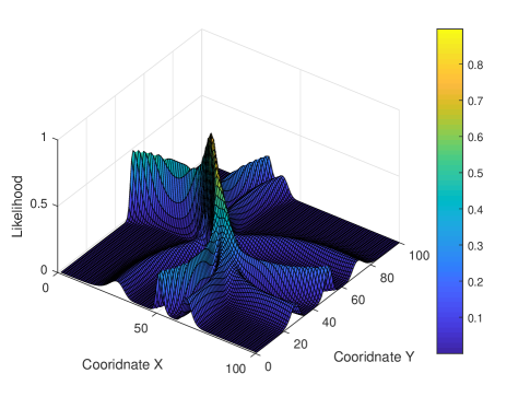
Figure 1: The log-likelihood distribution illustration with perfect channel parameters and $M=5$

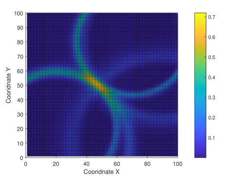
Figure 2: The topview of log-likelihood distribution illustration with perfect channel parameters and $M=5$

Fig.1 and Fig.2 compellingly unveil the intricate interplay between the target node’s location and the log-likelihood function. The numerical results reveal a two-tier fact. On one hand, the precise determination of the target node’s location hinges on the application of multilateration, utilizing the sensor-target distances as depicted in Fig.1 and Fig.2. Nevertheless, the acquisition of accurate sensor-target distances poses a significant challenge, attributed to the presence of correlated unknown noise and the imperfect locations of sensor nodes. On the other hand, the inherent complexity of the nonlinear and multimodal log-likelihood function brings great difficulty to direct maximization with low complexity, underscoring the need for efficient approaches in addressing this intricate relationship. In our pursuit of extracting maximum benefits from prior information, optimizing likelihood distributions, and achieving heightened precision in estimation solutions, we strategically embrace the foundational principle of Bayesian estimation. This approach not only empowers us to integrate existing knowledge effectively but also facilitates a comprehensive exploration of uncertainties, leading to more robust estimations. By leveraging the Bayesian framework, we tackle the intricacies of the estimation process with a posterior perspective, ensuring a thorough incorporation of available information for enhanced accuracy and reliability of our algorithm.

By considering the prior information of the unknown parameters and the Bayesian rule, the posterior distribution can be given by

$$p\left({\gamma,\delta_{0},{\boldsymbol{x}},{{\boldsymbol{x}}_{1:N}}|\boldsymbol{r}}\right)\propto$$ (3)

$$p\left({{\boldsymbol{r}}\mid{\boldsymbol{x}},{{\boldsymbol{x}}_{1:N}},\gamma,\delta_{0}}\right)p\left(\gamma\right)p\left({\boldsymbol{x}}\right)p\left(\delta_{0}\right)\prod\limits_{i=1}^{N}p\left({{{\boldsymbol{x}}_{i}}}\right),$$

and the estimation of the unknown parameters can be obtained via the following maximization

$${\boldsymbol{\hat{\Theta}}}=\arg\max p\left({{\boldsymbol{\Theta}}|{\boldsymbol{r}}}\right),$$ (4)

where ${\boldsymbol{\Theta}}=\left[{\boldsymbol{x}},{{\boldsymbol{x}}_{1:N}},{\gamma,{\Lambda}_{0}}\right]$ and ${\Lambda_{0}}={\delta}^{-2}_{0}$.

Given the measurements from all sensor nodes, the target node location and the channel can be theoretically estimated in (4). In the paper, we focus on the joint estimation of the target node location, the fading parameter $\gamma$ and noise reference power $\delta_{0}$ with the distance-dependent noise and sensor node location errors. The direct maximization of the likelihood function in (2) and the posterior distribution in (4) are intractable due to the nonlinear distance, unknown noise variance and coupled unknown parameters. To obtain the solutions to the joint estimation and localization problem, we proposed a variational message passing-based joint localization and channel estimation algorithm.

III Variational Bayesian Learning Framework

Based on the formulated problem in (4), the goal of direct estimation the unknown parameters is not tractable. Therefore, we aim at finding an approximation distribution to the true posterior distribution and find the estimation of the unknown parameters. In the section, we propose a variational message passing-based joint localization and channel estimation algorithm under the variational Bayesian learning framework.

In the Bayesian learning framework, the complicated and intractable posterior distribution motivate us to find a distribution $q({\boldsymbol{\Theta}})$ to approximate the true posterior distribution $p({\boldsymbol{\Theta}}|{\boldsymbol{r}})$. Meanwhile, the variational distribution $q({\boldsymbol{\Theta}})$ should be tractable. By assuming the independence between variational distributions of unknown parameters and the mean-field theory, the variational distribution $q({\boldsymbol{\Theta}})$ can be factorized as

$$q\left({\boldsymbol{\Theta}}\right)=\prod\limits_{{{\boldsymbol{\Theta}}_{k}}\in{\boldsymbol{\Theta}}}{q\left({{{\boldsymbol{\Theta}}_{k}}}\right)},$$ (5)

Meanwhile, the Kullback-Leibler (KL) divergence [38] is introduced to evaluate the information distance between the variational distribution $q({\boldsymbol{\Theta}})$ and the true distribution $p({\boldsymbol{\Theta}}|{\boldsymbol{R}})$, which is given by

$${\text{KL}}\left({q\left({\boldsymbol{\Theta}}\right)||p\left({\boldsymbol{\Theta}}|{\boldsymbol{r}}\right)}\right)=-{\mathbb{E}_{q\left({\boldsymbol{\Theta}}\right)}}\left\{{\ln\frac{{p\left({\boldsymbol{\Theta}}|{\boldsymbol{r}}\right)}}{{q\left({\boldsymbol{\Theta}}\right)}}}\right\}\geq 0,$$ (6)

where ${\mathbb{E}_{q\left({\boldsymbol{\Theta}}\right)}}$ is the expectation with respect to ${q\left({\boldsymbol{\Theta}}\right)}$ and the equality holds only when $q\left({\boldsymbol{\Theta}}\right)=p\left({\boldsymbol{\Theta}}|{\boldsymbol{r}}\right)$ as shown in [36].

By substituting the mean-field factorization in (5) into the Kullback-Leibler (KL) divergence in (6) and applying alternative optimization method the variational distribution $q^{(\xi)}\left({{{\boldsymbol{\Theta}}_{k}}}\right)$ can be iteratively given by [38]

$$q^{(\xi)}\left({{{\boldsymbol{\Theta}}_{k}}}\right)\propto\exp\left\{{{\mathbb{E}_{{q^{(\xi)}\left({{{\boldsymbol{\Theta}}_{\backslash k}}}\right)}}}\left[{\ln p\left({{\boldsymbol{\Theta}},{\boldsymbol{r}}}\right)}\right]}\right\},$$ (7)

where $q^{(\xi)}\left({{{\boldsymbol{\Theta}}_{k}}}\right)$ is the the $\xi$-th approximation to the true posterior distribution $p\left({{{\bf{\Theta}}_{k}}|{\boldsymbol{r}}}\right)$ and $p\left({{\boldsymbol{\Theta}},{\boldsymbol{r}}}\right)$ is the joint probability. ${\mathbb{E}_{{q^{(\xi)}}\left({{{\boldsymbol{\Theta}}_{\backslash k}}}\right)}}$ means the expectation with respect the variational distributions excluding the variational distribution $q^{(\xi)}\left({{{\boldsymbol{\Theta}}_{k}}}\right)$. The variational distribution in (7) will approximate the true posterior distribution iteratively and the approximated distribution ${q\left({{{\boldsymbol{\Theta}}_{k}}}\right)}$ is treated as the approximation of the corresponding posterior distribution $p\left({\boldsymbol{\Theta}}_{k}|{\boldsymbol{r}}\right)$. For example, $q\left(\gamma\right)$ is the approximation to the posterior distribution $p\left({\gamma|{\boldsymbol{r}}}\right)$.

Then the estimation of parameter ${{\boldsymbol{\Theta}}_{k}}$ can be obtained via maximum a posterior(MAP) as

$${{\boldsymbol{\Theta}}^{{\text{MAP}}}_{k}}={\mathop{\rm argmax}\nolimits}\;{q\left({{{\boldsymbol{\Theta}}_{k}}}\right)}.$$ (8)

In order to find the tractable forms of variational distribution $q\left({{{\boldsymbol{\Theta}}}}\right)$, we assume the prior distributions and the variational distribution follows the conjugate prior principles, which guarantees the variational distribution $q^{(\xi)}\left({{{\boldsymbol{\Theta}}_{k}}}\right)$ is identical to the prior distribution $p\left({{{\boldsymbol{\Theta}}_{k}}}\right)$ in form, i.e., $p\left(\gamma\right)$ is a Gaussian distribution with ${\cal N}\left({\gamma|{\mu_{\gamma}},{\delta_{\gamma}}}\right)$ then the $\xi$-th variational distribution $q^{(\xi)}\left(\gamma\right)$ is also a Gaussian distribution with $\mathcal{N}\left({\gamma|{\mu^{\left(\xi\right)}_{\gamma}},\delta_{\gamma}^{\left(\xi\right)}}\right)$ and other prior distributions are clarified as following:

• For the reference noise power $\delta_{0}$, the theoretical results signify that its inverse variable $\Lambda_{0}$ can be modeled as a gamma distribution and is given by

  $$p\left({{\Lambda_{0}}}\right)=\Gamma\left({{\Lambda_{0}}|a,b}\right).$$ (9)

• The sensor node locations are assumed to be known with location uncertainty and are modeled as

  $$p\left({{{\boldsymbol{x}}_{i}}}\right)=\mathcal{N}\left({{{\boldsymbol{x}}_{i}}|{{\bar{\boldsymbol{x}}}_{i}},{\boldsymbol{\Sigma}_{i}}}\right),$$ (10)

  where ${{\bar{\boldsymbol{x}}}_{i}}$ is the known coarse location and ${\boldsymbol{\Sigma}_{i}}$ is the covariance matrix.

• The prior distribution of the target node location is also assumed to be a Gaussian distribution with $p\left({{{\boldsymbol{x}}}}\right)=\mathcal{N}\left({{{\boldsymbol{x}}}|{{\bar{\boldsymbol{x}}}},{\boldsymbol{\Sigma}}}\right)$ and ${{\bar{\boldsymbol{x}}}}$ is the known coarse location and ${\boldsymbol{\Sigma}}$ is the covariance matrix.

Considering the vast complexity of repetitive and boring computation with the joint distribution $p\left({{\boldsymbol{\Theta}},{\boldsymbol{r}}}\right)$, we further build a probabilistic graphical model and map the dependencies between the variables in the directed graph. As shown in Fig.1, the variables are represented by nodes in the directed graph and the nodes are connected by the directed edges, which are the conditional dependencies between the variables. Moreover, the nodes can be classified into parent nodes ${\cal P}_{{\boldsymbol{\Theta}_{k}}}$ and child nodes ${{\cal C}_{{\boldsymbol{\Theta}_{k}}}}$ for a variable node ${\boldsymbol{\Theta}_{k}}$ according to Bayeisan graphical theory. For example, the node $a$ and node $b$ from the prior distribution (9) are the parent nodes ${\cal P}_{\Lambda_{0}}$ and node $\boldsymbol{r}$ from the likelihood function is the child node ${\cal C}_{\Lambda_{0}}$ of parameter ${\Lambda_{0}}$ respectively. Using the Bayeisan graphical representation, the marginal probability $p\left({{\boldsymbol{\Theta}_{k}}|{{\cal P}_{{\boldsymbol{\Theta}_{k}}}}}\right)$ and the conditional dependencies $p\left({{{\cal C}_{{\boldsymbol{\Theta}_{k}}}}|{\boldsymbol{\Theta}_{k}},{\boldsymbol{\Theta}_{m}}}\right)$, joint probability distribution $p\left({{\boldsymbol{\Theta}},{\boldsymbol{r}}}\right)$ can be reformulated.

Invoked by the fact that the prior distributions and likelihood distribution in the probabilistic graphical model all follow the form of exponential functions, we can reformulate the conditional distributions as

$$p\left({{\boldsymbol{\Theta}_{k}}|{{\cal P}_{{\boldsymbol{\Theta}_{k}}}}}\right)\propto\exp\left[{{{\cal J}_{{\boldsymbol{\Theta}_{k}}}}\left({{{\cal P}_{{\boldsymbol{\Theta}_{k}}}}}\right)\mathcal{G}\left({{\boldsymbol{\Theta}_{k}}}\right)+{\mathcal{F}}\left({{\boldsymbol{\Theta}_{k}}}\right)}\right],$$ (11)

$$p\left({{{\cal C}_{{\boldsymbol{\Theta}_{k}}}}|{\boldsymbol{\Theta}_{k}},{\boldsymbol{\Theta}_{m}}}\right)\propto\exp\left[{{\mathcal{J}_{{\boldsymbol{\Theta}_{k}}}}\left({{\boldsymbol{\Theta}_{m}},{{\cal C}_{{\boldsymbol{\Theta}_{k}}}}}\right)\mathcal{G}\left({{\boldsymbol{\Theta}_{k}}}\right)+\mathcal{B}\left({{{\cal C}_{{\boldsymbol{\Theta}_{k}}}}}\right)}\right],$$ (12)

where $\mathcal{F}\left(\cdot\right)$ and $\mathcal{B}\left(\cdot\right)$ mean the functions only associated with the corresponding variables. ${{{\cal J}_{{\boldsymbol{\Theta}_{k}}}}\left({{{\cal P}_{{\Theta_{k}}}}}\right)}$ and ${{{\cal J}_{{\boldsymbol{\Theta}_{k}}}}\left({{\boldsymbol{\Theta}_{m}},{{\cal C}_{{\boldsymbol{\Theta}_{k}}}}}\right)}$ are the natural sufficient statistics of the corresponding exponential family distributions. Given the natural sufficient statistics, the first moment and second moment of the distribution are known. The natural sufficient statistics expressions change with different variables and will be illustrated in following subsection.

Substituting (11) and (12) into (7), it yields

$${q^{(\xi)}}\left({{{\boldsymbol{\Theta}}_{k}}}\right)\propto\exp\left\{{{{\cal Q}_{{{\boldsymbol{\Theta}}_{k}}}^{\left({\xi}\right)}}\mathcal{G}\left({{\boldsymbol{\Theta}_{k}}}\right)+\mathcal{F}\left({{\boldsymbol{\Theta}_{k}}}\right)}\right\},$$ (13)

where ${{\cal Q}_{{{\boldsymbol{\Theta}}_{k}}}^{\left({\xi}\right)}}$ is the $\xi$-th estimated natural statistics of the distribution ${q^{(\xi)}}\left({{{\boldsymbol{\Theta}}_{k}}}\right)$. Intuitively, the iterative update of the variational distribution ${q^{(\xi)}}\left({{{\boldsymbol{\Theta}}_{k}}}\right)$ only depends on the update of the term ${{\cal Q}_{{{\boldsymbol{\Theta}}_{k}}}^{\left({\xi}\right)}}$ and it can be partitioned into two different terms:

$${\mathcal{Q}^{(\xi)}_{{{\boldsymbol{\Theta}}_{k}}}} =\underbrace{{\mathbb{E}_{\prod\limits_{j\neq k}{q^{(\xi)}\left({{{\boldsymbol{\Theta}}_{j}}}\right)}}}\left[{{\mathcal{J}_{{\boldsymbol{\Theta}_{k}}}}\left({\mathcal{P}_{{\boldsymbol{\Theta}}_{k}}}\right)}\right]}_{\mathcal{Q}^{\left(\xi\right)}_{{\mathcal{P}_{{\boldsymbol{\Theta}}_{k}}}\rightarrow{{\boldsymbol{\Theta}}_{k}}}}$$ (14)

$$+\sum\limits_{\mathcal{C}_{{\boldsymbol{\Theta}}_{k}}}\underbrace{{{\mathbb{E}_{\prod\limits_{j\neq k}{q^{(\xi)}\left({{{\boldsymbol{\Theta}}_{j}}}\right)}}}\left[{{\mathcal{J}_{{\boldsymbol{\Theta}_{k}}}}\left({{{\boldsymbol{\Theta}}_{m}},{\mathcal{C}_{{\boldsymbol{\Theta}}_{k}}}}\right)}\right]}}_{\mathcal{Q}^{\left(\xi\right)}_{{\mathcal{C}_{{\boldsymbol{\Theta}}_{k}}}\rightarrow{{\boldsymbol{\Theta}}_{k}}}},$$

where the first subterm ${\mathcal{Q}^{\left(\xi\right)}_{{\mathcal{P}_{{\boldsymbol{\Theta}}_{k}}}\rightarrow{{\boldsymbol{\Theta}}_{k}}}}$ is the message from the parent node ${\mathcal{P}_{{\boldsymbol{\Theta}}_{k}}}$ and the second subterm ${\mathcal{Q}^{\left(\xi\right)}_{{\mathcal{C}_{{\boldsymbol{\Theta}}_{k}}}\rightarrow{{\boldsymbol{\Theta}}_{k}}}}$ is the message from the child node ${\mathcal{C}_{{\boldsymbol{\Theta}}_{k}}}$.

Given the message update in (14), the original cumbersome distribution iterations are reduced to the lightweight message update between the nodes in the directed graph in Fig.3. Specifically, the messages are essentially the expectations of the natural sufficient statistics of the prior distributions and the likelihood distribution. Given the messages from the neighboring nodes, the natural sufficient statistics of the posterior distributions can be updated iteratively. Given the message update scheme, the natural sufficient statistics of the variational distributions $q\left({{\boldsymbol{\Theta}}_{k}}\right)$ are obtained iteratively. However, it is too complicated to obtain closed-form solutions and the derivations of the messages are still non-trivial and still challenging due to the unknown fading parameter and the unknown distance-dependent noise. In the following subsections, the detailed theoretical derivations of the messages are presented.

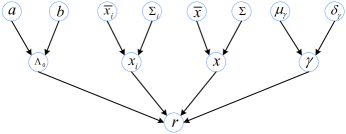
Figure 3: The probabilistic graph of the joint probability

IV Joint Localization and Channel Estimation Algorithm

Using the message passing scheme, the unknown parameters are estimated via the updated messages from the parent nodes and the child nodes. In the following, we present the message update and the estimation of unknown parameters in details.

IV-A Estimation of path loss exponent parameter $\gamma$

To find the estimation of the unknown parameter $\gamma$, it is required to get the estimation of the natural sufficient statistics $\mathcal{Q}_{\gamma}^{\left({\xi}\right)}$ of the variational distribution ${q^{\left({\xi}\right)}}\left(\gamma\right)$. According to (14), the message $\mathcal{Q}_{{\mathcal{P}_{\gamma}}\to\gamma}^{\left({\xi}\right)}$ from its parent nodes ${{\mu_{\gamma}}}$ and ${{\delta_{\gamma}}}$ and the message $\mathcal{Q}_{\boldsymbol{r}\to\gamma}^{\left({\xi}\right)}$ from its child node $\boldsymbol{r}$ are derived respectively.

Message $\mathcal{Q}_{{\mathcal{P}_{\gamma}}\to\gamma}^{\left({\xi}\right)}$: In Fig.3, the message $\mathcal{Q}_{{\mathcal{P}_{\gamma}}\to\gamma}^{\left({\xi}\right)}$ from parent nodes ${{\mu_{\gamma}}}$ and ${{\delta_{\gamma}}}$ is related to the prior distribution ${\cal N}\left({\gamma|{\mu_{\gamma}},{\delta_{\gamma}}}\right)$. By applying (11) to the prior distribution of $\gamma$, the prior distribution of $\gamma$ can be rewritten as

$$p\left(\gamma\right)=\exp\left({\left[{\begin{array}[]{*{20}{c}}{\frac{{{\mu_{\gamma}}}}{{{\delta_{\gamma}}}}}&{-\frac{1}{{2{\delta_{\gamma}}}}}\end{array}}\right]\left[{\begin{array}[]{*{20}{c}}\gamma\\ {{\gamma^{2}}}\end{array}}\right]}\right)+{\cal C},$$ (15)

Comparing with the expression in (11), we can obtain the natural sufficient statistics of $\gamma$ as ${\mathcal{J}_{\mathcal{\gamma}}}\left({{\mathcal{P}_{\gamma}}}\right)=\left[{\begin{array}[]{*{20}{c}}{\frac{{{\mu_{\gamma}}}}{{{\delta_{\gamma}}}}}&-{\frac{1}{{2{\delta_{\gamma}}}}}\end{array}}\right]$ and $\mathcal{G}\left(\gamma\right)=\left[{\begin{array}[]{*{20}{c}}\gamma\\ {{\gamma^{2}}}\end{array}}\right]$. By substituting the prior distribution of $\gamma$ into (14) , the message $\mathcal{Q}_{{\mathcal{P}_{\gamma}}\to\gamma}^{\left({\xi}\right)}$ can be given by

$$\mathcal{Q}_{{{\cal P}_{\gamma}}{\to\gamma}}^{\left(\xi\right)}=\left[{\begin{array}[]{*{20}{c}}{\frac{{{\mu_{\gamma}}}}{{{\delta_{\gamma}}}}}&-{\frac{1}{{2{\delta_{\gamma}}}}}\end{array}}\right].$$ (16)

Message $\mathcal{Q}_{\boldsymbol{r}\to\gamma}^{\left({\xi}\right)}$: The message $\mathcal{Q}_{\boldsymbol{r}\to\gamma}^{\left({\xi}\right)}$ from the child node $\boldsymbol{r}$ to node $\gamma$ involves the likelihood function in (2) and the likelihood function with respect to the parameter $\gamma$ can be given by

$$p\left({{\boldsymbol{r}}\mid{\boldsymbol{\Theta}}}\right)\propto\exp\left({-\sum_{i=1}^{N}\frac{\gamma}{2}\ln{d_{i}}-\sum_{i=1}^{N}\frac{{{{\left({{r_{i}}-{d_{i}}}\right)}^{2}}{\Lambda_{0}}}}{{2d_{i}^{\gamma}}}}\right).$$ (17)

Due to the nonlinear unknown parameter $\gamma$ in the second term in (17), it is intractable to present the direct reformulation by following (12). Hence, we apply Taylor expansion to linearize the likelihood function with respect to the parameter $\gamma$. By denoting $g\left(\gamma\right)=\sum\limits_{i=1}^{N}{{{\left({{g_{i}}\left(\gamma\right)}\right)}^{2}}}=\sum\limits_{i=1}^{N}{{{\left({\frac{{{r_{i}}-{d_{i}}}}{{d_{i}^{\frac{\gamma}{2}}}}}\right)}^{2}}}$, the Taylor expansion of $g\left(\gamma\right)$ can be given by

$$\begin{aligned} &g\left(\gamma\right)\\ &\approx\sum\limits_{i=1}^{N}{{{\left({{g_{i}}\left({{\gamma^{\left(\xi\right)}}}\right)+{\boldsymbol{\Delta}}_{\gamma,i}\left({\gamma-{\gamma^{\left(\xi\right)}}}\right)}\right)}^{2}}}\\ &=\sum\limits_{i=1}^{N}{{{\left({{\boldsymbol{\Delta}}_{\gamma,i}}\right)}^{2}}}{\gamma^{2}}-2\sum\limits_{i=1}^{N}{{\boldsymbol{\Delta}}_{\gamma,i}\left({{\gamma^{\left(\xi\right)}}-{g_{i}}\left({{\gamma^{\left(\xi\right)}}}\right)}\right)}\gamma+\mathcal{C}\\ \end{aligned},$$ (18)

where ${\boldsymbol{\Delta}}_{\gamma,i}^{\left(\xi\right)}=-\frac{1}{2}\left({{r_{i}}-{d_{i}}}\right)d_{i}^{-\frac{\gamma}{2}}\ln{d_{i}}$ is the derivative with respect to $\gamma$. Hence, substituting (18) into (12) and (17), it yields

$$p\left({{\boldsymbol{r}}\mid{\boldsymbol{\Theta}}}\right)\propto\exp\left(\left[{\begin{array}[]{*{20}{c}}{{\boldsymbol{\mathcal{U}}_{\gamma}}}&{-\frac{{1}}{2}}{\boldsymbol{\cal A}_{\gamma}}\end{array}}\right]\left[{\begin{array}[]{*{20}{c}}\gamma\\ {{\gamma^{2}}}\end{array}}\right]\right),$$ (19)

where ${{\boldsymbol{\cal A}}_{\gamma}}=\sum\limits_{i=1}^{N}{{{\left({{\boldsymbol{\Delta}}_{\gamma,i}}\right)}^{2}}}\Lambda_{0}=\sum\limits_{i=1}^{N}\frac{1}{4}{{{\left({\frac{{{r_{i}}-{d_{i}}}}{{d_{i}^{{\gamma\mathord{\left/{{2}}\right.}}}}}\ln{d_{i}}}\right)}^{2}}}\Lambda_{0}$ and ${{\boldsymbol{\cal U}}_{\gamma}}=\sum\limits_{i=1}^{N}{{{\left({{\boldsymbol{\Delta}}_{\gamma,i}}\right)}^{2}}{{\boldsymbol{\Theta}}_{\gamma,i}}}$ with ${\boldsymbol{\Theta}}_{\gamma,i}={{\gamma^{\left(\xi\right)}}{\Lambda_{0}}-{g_{i}}\left({{\gamma^{\left(\xi\right)}}}\right){\Lambda_{0}}-\frac{1}{4}\ln{d_{i}}}$.

Therefore, the natural sufficient statistics of $\gamma$ in (2) can be given by ${{\cal J}_{\gamma}}\left(\boldsymbol{r}\right)=\left[{\begin{array}[]{*{20}{c}}{{\boldsymbol{\cal U}_{\gamma}}}&-{\frac{1}{2}{\boldsymbol{\mathcal{A}}_{\gamma}}}\end{array}}\right]$. Then plugging the natural sufficient statistics into (14), it yields

$${\cal Q}_{{\boldsymbol{r}}\to\gamma}^{\left({\xi}\right)}={\mathbb{E}_{{q^{\left(\xi\right)}}\left({{\boldsymbol{\Theta}_{\backslash\gamma}}}\right)}}\left[{{{\cal J}_{\gamma}}\left(\boldsymbol{r}\right)}\right]=\left[{\begin{array}[]{*{20}{c}}{\boldsymbol{\cal U}_{\gamma}^{\left(\xi\right)}}&-{\frac{1}{2}\boldsymbol{\mathcal{A}}_{\gamma}^{\left(\xi\right)}}\end{array}}\right],$$ (20)

where

$$\boldsymbol{\cal A}_{\gamma}^{\left(\xi\right)} ={\mathbb{E}_{{q^{\left(\xi\right)}}\left({{{\boldsymbol{\Theta}}_{\backslash\gamma}}}\right)}}\left({{\boldsymbol{\cal A}_{\gamma}}}\right)$$ (21)

$$\approx\sum\limits_{i=1}^{N}{{{\left({\frac{{{r_{i}}-d_{i}^{\left(\xi\right)}}}{{{{\left({d_{i}^{\left(\xi\right)}}\right)}^{\frac{{{\gamma^{\left(\xi\right)}}}}{2}}}}}\ln d_{i}^{\left(\xi\right)}}\right)}^{2}}}\frac{{{a^{\left(\xi\right)}}}}{{{b^{\left(\xi\right)}}}}$$

The approximation holds by applying the Taylor expansion at ${\boldsymbol{x}}^{\left(\xi\right)}$ and ${\boldsymbol{x}}_{i}^{\left(\xi\right)}$, which are obtained via the $\xi$-th estimation of target node location and sensor node locations respectively. where ${a^{\left(\xi\right)}}$ and ${b^{\left(\xi\right)}}$ are the parameters in ${q^{\left(\xi\right)}}\left({{\Lambda_{0}}}\right)=\Gamma\left({{\Lambda_{0}}|{a^{\left(\xi\right)}},{b^{\left(\xi\right)}}}\right)$ which will be introduced later in subsection III-B. The parameter $\boldsymbol{\cal U}_{\gamma}^{\left(\xi\right)}$ is given by

$${\boldsymbol{\cal U}}_{\gamma}^{\left(\xi\right)}={\mathbb{E}_{{q^{\left(\xi\right)}}\left({{{\boldsymbol{\Theta}}_{\backslash\gamma}}}\right)}}\left({{{\boldsymbol{\cal U}}_{\gamma}}}\right)\approx\sum\limits_{i=1}^{N}{{{\left({{\boldsymbol{\Delta}}_{\gamma,i}^{\left(\xi\right)}}\right)}^{2}}{\boldsymbol{\Theta}}_{\gamma,i}^{\left(\xi\right)}},$$ (22)

where ${\boldsymbol{\Theta}}_{\gamma,i}^{\left(\xi\right)}={\gamma^{\left(\xi\right)}}\frac{{{a^{\left(\xi\right)}}}}{{{b^{\left(\xi\right)}}}}-{g_{i}}\left({{\gamma^{\left(\xi\right)}}}\right)\frac{{{a^{\left(\xi\right)}}}}{{{b^{\left(\xi\right)}}}}-\frac{1}{4}\ln d_{i}^{\left(\xi\right)}$ and ${\mathbb{E}_{{q^{\left(\xi\right)}}\left({{\boldsymbol{\Theta}_{\backslash\gamma}}}\right)}}\left({\ln{d_{i}}}\right)=\ln d_{i}^{\left(\xi\right)}$ in [37] with $d_{i}^{\left(\xi\right)}={\left\|{{\boldsymbol{x}^{\left(\xi\right)}}-\boldsymbol{x}_{i}^{\left(\xi\right)}}\right\|_{2}}$.

Invoked by the conjugate prior principle, the variational distribution $q\left(\gamma\right)$ is also a Gamma distribution. By plugging (16) and (22) into (14), it yields

$${\cal Q}_{\gamma}^{(\xi)} =\left[{\begin{array}[]{*{20}{c}}{\frac{{\mu_{\gamma}^{\left({\xi}\right)}}}{{\delta_{\gamma}^{\left({\xi}\right)}}}}&{-\frac{1}{{2\delta_{\gamma}^{\left({\xi}\right)}}}}\end{array}}\right]$$ (23)

$$=\left[{\begin{array}[]{*{20}{c}}{\frac{{{\mu_{\gamma}}}}{{{\delta_{\gamma}}}}+\boldsymbol{\mathcal{U}}_{\gamma}^{\left(\xi\right)}}&{-\frac{1}{{2{\delta_{\gamma}}}}-\frac{1}{2}\boldsymbol{\cal A}_{\gamma}^{\left(\xi\right)}}\end{array}}\right].$$

Hence, the $\xi$-th mean and variance of $\gamma$ can be respectively given by

$$\delta_{\gamma}^{\left({\xi}\right)}={\left({\frac{1}{{{\delta_{\gamma}}}}+\boldsymbol{\cal A}_{\gamma}^{\left(\xi\right)}}\right)^{-1}},$$ (24)

$$\mu_{\gamma}^{\left({\xi}\right)}=\delta_{\gamma}^{\left({\xi}\right)}\left({\frac{{{\mu_{\gamma}}}}{{{\delta_{\gamma}}}}+\boldsymbol{\mathcal{U}}_{\gamma}^{\left(\xi\right)}}\right).$$ (25)

Thus, the $\xi$-th estimation of $\gamma$ can be obtained via (25). Intuitively, the natural sufficient statistics $\mathcal{Q}_{\gamma}^{\left({\xi}\right)}$, $\mathcal{Q}_{{\mathcal{P}_{\gamma}}\to\gamma}^{\left({\xi}\right)}$ and $\mathcal{Q}_{\boldsymbol{r}\to\gamma}^{\left({\xi}\right)}$ are the means and variances of the their distributions and the messages are the expectations of means and variances.

IV-B Estimation of fading parameter $\Lambda_{0}$

In order to estimate the unknown parameter $\Lambda_{0}$, it is required to estimate the natural sufficient statistics $\mathcal{Q}_{\Lambda_{0}}^{\left({\xi}\right)}$ of the variational distribution ${q^{\left({\xi}\right)}}\left({\Lambda_{0}}\right)$. Similarly, the message $\mathcal{Q}_{{\mathcal{P}_{\Lambda_{0}}}\to{\Lambda_{0}}}^{\left({\xi}\right)}$ from its parent nodes ${{a}}$ and ${{b}}$ and the message $\mathcal{Q}_{\boldsymbol{r}\to{\Lambda_{0}}}^{\left({\xi}\right)}$ from its child node $\boldsymbol{r}$ are also derived respectively.

Message $\mathcal{Q}_{{\mathcal{P}_{\Lambda_{0}}}\to{\Lambda_{0}}}^{\left({\xi}\right)}$: The message $\mathcal{Q}_{{\mathcal{P}_{\Lambda_{0}}}\to{\Lambda_{0}}}^{\left({\xi}\right)}$ involves the parent nodes $a$ and $b$ which is given in the prior distribution (9). By following (11), the prior distribution of ${\Lambda_{0}}$ can be rewritten as

$$p\left({\left.{{\Lambda_{0}}}\right|a,b}\right) \propto\exp\left({\left({a-1}\right)\ln{\Lambda_{0}}-b{\Lambda_{0}}}\right)$$ (26)

$$=\exp\left({\left[{\begin{array}[]{*{20}{c}}{a-1}&-b\end{array}}\right]\left[{\begin{array}[]{*{20}{c}}{{\Lambda_{0}}}\\ {\ln{\Lambda_{0}}}\end{array}}\right]}\right),$$

Therefore, the natural sufficient statistics of ${\Lambda_{0}}$ is given by ${\mathcal{J}_{\Lambda_{0}}}\left({{\mathcal{P}_{\Lambda_{0}}}}\right)={\left[{\begin{array}[]{*{20}{c}}{a-1}&b\end{array}}\right]}$ and $\mathcal{G}\left({\Lambda_{0}}\right)=\left[{\begin{array}[]{*{20}{c}}{\Lambda_{0}}\\ {{\ln{\Lambda_{0}}}}\end{array}}\right]$. By substituting the natural sufficient statistics of ${\Lambda_{0}}$ into (14), the message $\mathcal{Q}_{{\mathcal{P}_{\Lambda_{0}}}\to{\Lambda_{0}}}^{\left({\xi}\right)}$ can be given by

$${\cal Q}_{{\mathcal{P}_{{\Lambda_{0}}}}\to{\Lambda_{0}}}^{\left({\xi}\right)}=\left[{\begin{array}[]{*{20}{c}}{a-1}&{-b}\end{array}}\right].$$ (27)

Message $\mathcal{Q}_{\boldsymbol{r}\to{\Lambda_{0}}}^{\left({\xi}\right)}$: According to (12), $\mathcal{Q}_{\boldsymbol{r}\to{\Lambda_{0}}}^{\left({\xi}\right)}$ is the message from the child node $\boldsymbol{r}$ and requires the exponential factorization of the likelihood function in (2), which is given by

$$p\left({{\boldsymbol{r}}\mid{\boldsymbol{\Theta}}}\right)\propto \exp\left({\frac{N}{2}\ln{\Lambda_{0}}-\sum\limits_{i=1}^{N}{\frac{{{{\left({{r_{i}}-{d_{i}}}\right)}^{2}}{\Lambda_{0}}}}{{2d_{i}^{\gamma}}}}}\right)$$ (28)

$$=\exp\left({\left[{\begin{array}[]{*{20}{c}}{{\mathcal{I}_{{\Lambda_{0}}}}}&\frac{N}{2}\end{array}}\right]\left[{\begin{array}[]{*{20}{c}}{{\Lambda_{0}}}\\ {\ln{\Lambda_{0}}}\end{array}}\right]}\right)+{\cal C},$$

where ${{\cal J}_{\Lambda_{0}}}\left(\boldsymbol{r}\right)={\left[{\begin{array}[]{*{20}{c}}{{\mathcal{I}_{{\Lambda_{0}}}}}&\frac{N}{2}\end{array}}\right]}$ is the natural sufficient statistics of ${\Lambda_{0}}$ involved in the likelihood and ${\mathcal{I}_{{\Lambda_{0}}}}=-\sum\limits_{i=1}^{N}{\frac{{{{\left({{r_{i}}-{d_{i}}}\right)}^{2}}}}{{2d_{i}^{\gamma}}}}$. According to (14), the $\mathcal{Q}_{\boldsymbol{r}\to{\Lambda_{0}}}^{\left({\xi}\right)}$ is the variational expectation of the natural sufficient statistics of ${\Lambda_{0}}$. But the natural sufficient statistics contains the nonlinear term and we also apply the Taylor expansion at the $\xi$-th estimation of $\boldsymbol{x}$, ${\boldsymbol{x}}_{i}$ and $\gamma$. Thus, the message $\mathcal{Q}_{\boldsymbol{r}\to{\Lambda_{0}}}^{\left({\xi}\right)}$ is given by

$$\mathcal{Q}_{\boldsymbol{r}\to{\Lambda_{0}}}^{\left({\xi}\right)} ={\mathbb{E}_{{q^{\left(\xi\right)}}\left({{\boldsymbol{\Theta}_{\backslash{\Lambda_{0}}}}}\right)}}\left[{{{\cal J}_{\Lambda_{0}}}\left(\boldsymbol{r}\right)}\right]$$ (29)

$$=\left[{\begin{array}[]{*{20}{c}}{\mathcal{I}_{{\Lambda_{0}}}^{\left({\xi+1}\right)}}&\frac{N}{2}\end{array}}\right],$$

where $\mathcal{I}_{{\Lambda_{0}}}^{\left({\xi}\right)}=-\sum\limits_{i=1}^{N}{\frac{{{{\left({{r_{i}}-d_{i}^{\left(\xi\right)}}\right)}^{2}}}}{{2{{\left({d_{i}^{\left(\xi\right)}}\right)}^{{\gamma^{\left(\xi\right)}}}}}}}$ by using similar operations in (18).

Substituting (29) and (26) into (14) yields,

$${\cal Q}_{{\Lambda_{0}}}^{(\xi)} =\mathcal{Q}_{{{\cal P}_{{\Lambda_{0}}}}\to{\Lambda_{0}}}^{\left({\xi}\right)}+{\cal Q}_{{\boldsymbol{r}}\to{\Lambda_{0}}}^{\left({\xi}\right)}$$ (30)

$$=\left[{\begin{array}[]{*{20}{c}}{a-1+\mathcal{I}_{{\Lambda_{0}}}^{\left({\xi}\right)}}&{-b+\frac{N}{2}}-1\end{array}}\right].$$

Thus, the $\xi$-th variational distribution of $\Lambda_{0}$ can be given by ${q^{\left({\xi}\right)}}\left({{\Lambda_{0}}|{a^{\left({\xi}\right)}},{b^{\left({\xi}\right)}}}\right)$. Combining it with (30), we can obtain ${a^{\left({\xi}\right)}}=a+\mathcal{I}_{{\Lambda_{0}}}^{\left({\xi}\right)}$ and ${b^{\left({\xi}\right)}}=b+\frac{N}{2}$ respectively.

Therefore, the $\xi$-th estimation of $\Lambda_{0}$ is given by

$$\Lambda_{0}^{\left({\xi}\right)}=\frac{{{a^{\left({\xi}\right)}}}}{{{b^{\left({\xi}\right)}}}}.$$ (31)

Different from the messages consisting of means and variances in subsection IV-A, the messages of $\Lambda_{0}$ are comprised of expectations of statistics parameters from the prior distribution in (9) and the likelihood distribution in (2). These messages update the statistics parameters leading to the iterative estimation of $\Lambda_{0}$.

IV-C Estimation of target node location ${\boldsymbol{x}}$

In this subsection, we focus on the estimation of the target node location ${\boldsymbol{x}}$. According to (14), the target node location estimation requires to iteratively update the natural sufficient statistics $\mathcal{Q}_{{\boldsymbol{x}}}^{\left({\xi}\right)}$ of the variational distribution ${q^{\left({\xi}\right)}}\left({\boldsymbol{x}}\right)$. Meanwhile, the message $\mathcal{Q}_{{\mathcal{P}_{{\boldsymbol{x}}}}\to{\boldsymbol{x}}}^{\left({\xi}\right)}$ from its parent nodes $\bar{\boldsymbol{x}}$ and ${\boldsymbol{\Sigma}}$ and the message $\mathcal{Q}_{\boldsymbol{r}\to{\Lambda_{0}}}^{\left({\xi}\right)}$ from its child node $\boldsymbol{r}$ are also derived respectively.

Message $\mathcal{Q}_{{\mathcal{P}_{{\boldsymbol{x}}}}\to{\boldsymbol{x}}}^{\left({\xi}\right)}$: According to the directed graph in Fig.1, the $\mathcal{Q}_{{\mathcal{P}_{{\boldsymbol{x}}}}\to{\boldsymbol{x}}}^{\left({\xi}\right)}$ is from its parent nodes $\bar{\boldsymbol{x}}$ and ${\boldsymbol{\Sigma}}$, which is generated from the prior distribution of ${\boldsymbol{x}}$. Substituting the prior distribution of ${\boldsymbol{x}}$ into (11) and simple trace manipulations, we can obtain

$$p\left({\boldsymbol{x}}\right)\propto \exp\left({tr\left({-\frac{1}{2}{{\left({{\boldsymbol{x}}-\bar{\boldsymbol{x}}}\right)}^{T}}{\boldsymbol{\Sigma}^{-1}}\left({{\boldsymbol{x}}-\bar{\boldsymbol{x}}}\right)}\right)}\right)$$ (32)

$$\propto \exp\left({tr\left({\left[{\begin{array}[]{*{20}{c}}{{{\left({\bar{\boldsymbol{x}}}\right)}^{T}}\boldsymbol{\Sigma}}&{-\frac{1}{2}\boldsymbol{\Sigma}^{-1}}\end{array}}\right]\left[{\begin{array}[]{*{20}{c}}{\boldsymbol{x}}\\ {{\boldsymbol{x}}{{\boldsymbol{x}}^{T}}}\end{array}}\right]}\right)}\right),$$

where $tr$ means the trace of a matrix and natural sufficient statistics of ${\boldsymbol{x}}$ in the prior distribution is given by ${{\cal J}_{{\boldsymbol{x}}}}\left({{{\cal P}_{\boldsymbol{x}}}}\right)=\left[{\begin{array}[]{*{20}{c}}{{{\left({\bar{\boldsymbol{x}}}\right)}^{T}}\boldsymbol{\Sigma}^{-1}}&{-\frac{1}{2}\boldsymbol{\Sigma}^{-1}}\end{array}}\right]$ with ${\cal G}\left({\boldsymbol{x}}\right)=\left[{\begin{array}[]{*{20}{c}}{\boldsymbol{x}}\\ {{\boldsymbol{x}}{{\boldsymbol{x}}^{T}}}\end{array}}\right]$. By substituting the natural sufficient statistics of ${\boldsymbol{x}}$ into (14), the message $\mathcal{Q}_{{\mathcal{P}_{{\boldsymbol{x}}}}\to{\boldsymbol{x}}}^{\left({\xi+1}\right)}$ can be given by

$${\cal Q}_{{{\cal P}_{\boldsymbol{x}}}\to{\boldsymbol{x}}}^{\left({\xi}\right)}=\left[{\begin{array}[]{*{20}{c}}{{{\left({\bar{\boldsymbol{x}}}\right)}^{T}}\boldsymbol{\Sigma}^{-1}}&{-\frac{1}{2}\boldsymbol{\Sigma}^{-1}}\end{array}}\right].$$ (33)

Message $\mathcal{Q}_{\boldsymbol{r}\to{\boldsymbol{x}}}^{\left({\xi}\right)}$: In (12), the message $\mathcal{Q}_{\boldsymbol{r}\to{\boldsymbol{x}}}^{\left({\xi}\right)}$ is derive from the likelihood function and the natural sufficient statistics requires linear combination of the involved unknown parameter in the likelihood function. Thus, we linearize the likelihood function with respect to the target node location ${\boldsymbol{x}}$. Firstly, the likelihood function can be rewritten as

$$\ln p\left({{\boldsymbol{r}}\mid{\boldsymbol{\Theta}}}\right)\propto-\sum\limits_{i=1}^{N}{\frac{\gamma}{2}}\ln{d_{i}}-\sum\limits_{i=1}^{N}{\frac{{{{\left({{r_{i}}-{d_{i}}}\right)}^{2}}{\Lambda_{0}}}}{{2d_{i}^{\gamma}}}},$$ (34)

where the likelihood function involves two nonlinear terms. By denoting ${h_{1}}\left({{\boldsymbol{x}},{{\boldsymbol{x}}_{i}}}\right)=\gamma\ln{d_{i}}$, ${h_{2}}\left({{\boldsymbol{x}},{{\boldsymbol{x}}_{i}}}\right)={\frac{{{r_{i}}-{d_{i}}}}{{d_{i}^{\gamma/2}}}}$ and applying Taylor expansion at $\left({{{\boldsymbol{x}}^{\left({\xi}\right)}},{\boldsymbol{x}}_{i}^{\left({\xi}\right)}}\right)$ which are respectively given by

$${h_{1}}\left({{\boldsymbol{x}},{{\boldsymbol{x}}_{i}}}\right)={{\gamma^{\left(\xi\right)}}}\ln d_{i}^{{}^{\left(\xi\right)}}+{\left({{{\boldsymbol{\omega}}^{\left(\xi\right)}_{i}}}\right)^{T}}\left({{\boldsymbol{x}}-{{\boldsymbol{x}}^{\left(\xi\right)}}}\right),$$ (35)

where ${{\boldsymbol{\omega}}^{\left(\xi\right)}_{i}}={{\gamma^{\left(\xi\right)}}\frac{1}{{d_{i}^{{}^{\left(\xi\right)}}}}{{\left.{\frac{{\partial{d_{i}}}}{{\partial{\boldsymbol{x}}}}}\right|}_{{{\boldsymbol{x}}^{\left(\xi\right)}},{\boldsymbol{x}}_{i}^{\left(\xi\right)}}}}$ and

$${h_{2}}\left({{\boldsymbol{x}},{{\boldsymbol{x}}_{i}}}\right)={\Upsilon^{\left(\xi\right)}_{i}}+{\left({{\boldsymbol{\Gamma}}_{i}^{\left(\xi\right)}}\right)^{T}}\left({{\boldsymbol{x}}-{{\boldsymbol{x}}^{\left(\xi\right)}}}\right),$$ (36)

where ${\Upsilon^{\left(\xi\right)}_{i}}$ and ${\boldsymbol{\Gamma}}_{i}^{\left(\xi\right)}$ are respectively given by

$${\Upsilon^{\left(\xi\right)}_{i}}={\frac{{{r_{i}}-d_{i}^{\left(\xi\right)}}}{{{{\left({d_{i}^{\left(\xi\right)}}\right)}^{{\gamma^{\left(\xi\right)}}/2}}}}},$$ (37)

$${\boldsymbol{\Gamma}}_{i}^{\left(\xi\right)}=-\frac{{1+0.5\gamma d_{i}^{-1}\left({{r_{i}}-{d_{i}}}\right)}}{{d_{i}^{\gamma/2}}}{\left.{\frac{{\partial{d_{i}}}}{{\partial{\boldsymbol{x}}}}}\right|_{{{\boldsymbol{x}}^{\left(\xi\right)}},{\boldsymbol{x}}_{i}^{\left(\xi\right)}}}.$$ (38)

Substituting (35) and (36) into (34) and taking exponential operation with both sides, it yields

$$p\left({{\boldsymbol{r}}\mid{\boldsymbol{\Theta}}}\right)\propto\exp\left({tr\left({-\frac{1}{2}{{\boldsymbol{x}}^{T}}{\boldsymbol{\Delta}}_{\boldsymbol{x}}^{\left(\xi\right)}{\boldsymbol{x}}+{{{\boldsymbol{U}}_{\boldsymbol{x}}^{\left(\xi\right)}}}{\boldsymbol{x}}}\right)}\right)$$ (39)

$$=\exp\left({tr\left({\left[{\begin{array}[]{*{20}{c}}{{{{\boldsymbol{U}}_{\boldsymbol{x}}^{\left(\xi\right)}}}}&{-\frac{1}{2}{\boldsymbol{\Delta}}_{\boldsymbol{x}}^{\left(\xi\right)}}\end{array}}\right]\left[{\begin{array}[]{*{20}{c}}{\boldsymbol{x}}\\ {{\boldsymbol{x}}{{\boldsymbol{x}}^{T}}}\end{array}}\right]}\right)}\right)$$

where ${{\cal J}_{\boldsymbol{x}}}\left({\boldsymbol{r}}\right)=\left[{\begin{array}[]{*{20}{c}}{{\boldsymbol{U}}_{\boldsymbol{x}}^{\left(\xi\right)}}&{-\frac{1}{2}{\boldsymbol{\Delta}}_{\boldsymbol{x}}^{\left(\xi\right)}}\end{array}}\right]$ is the natural sufficient statistics of ${\boldsymbol{x}}$ involved in the likelihood function and ${\boldsymbol{\Delta}}_{\boldsymbol{x}}^{\left(\xi\right)}$ and ${{\boldsymbol{U}}_{\boldsymbol{x}}^{\left(\xi\right)}}$ are respectively given by

$${\boldsymbol{\Delta}}_{\boldsymbol{x}}^{\left(\xi\right)}=\Lambda_{0}\sum\limits_{i=1}^{N}{{{\left({{\boldsymbol{\Gamma}}_{i}^{\left(\xi\right)}}\right)}^{T}}{\boldsymbol{\Gamma}}_{i}^{\left(\xi\right)}},$$ (40)

$${\boldsymbol{U}}_{\boldsymbol{x}}^{\left(\xi\right)} =\Lambda_{0}{\left({{{\boldsymbol{x}}^{\left(\xi\right)}}}\right)^{T}}\sum\limits_{i=1}^{N}{{{\left({{\boldsymbol{\Gamma}}_{i}^{\left(\xi\right)}}\right)}^{T}}{\boldsymbol{\Gamma}}_{i}^{\left(\xi\right)}}-\sum\limits_{i=1}^{N}\Lambda_{0}{\left({{\boldsymbol{\Gamma}}_{i}^{\left(\xi\right)}}\right)^{T}}{\Upsilon^{\left(\xi\right)}_{i}}$$ (41)

$$+\sum\limits_{i=1}^{N}\Lambda_{0}{\left({{{\boldsymbol{\omega}}^{\left(\xi\right)}_{i}}}\right)^{T}}.$$

The message $\mathcal{Q}_{\boldsymbol{r}\to{\boldsymbol{x}}}^{\left({\xi}\right)}$ can be obtained as

$${\cal Q}_{{\boldsymbol{r}}\to{\boldsymbol{x}}}^{\left({\xi}\right)}={\mathbb{E}_{{q^{\left(\xi\right)}}\left({{{\boldsymbol{\Theta}}_{\backslash{{\boldsymbol{x}}}}}}\right)}}\left[{{\mathcal{J}_{\boldsymbol{x}}}\left({\boldsymbol{r}}\right)}\right]=\left[{\begin{array}[]{*{20}{c}}{\mathcal{U}_{\boldsymbol{x}}^{\left({\xi}\right)}}&{-\frac{1}{2}\mathcal{A}_{\boldsymbol{x}}^{\left({\xi}\right)}}\end{array}}\right],$$ (42)

where ${\mathcal{U}_{\boldsymbol{x}}^{\left({\xi}\right)}}$ and $\mathcal{A}_{\boldsymbol{x}}^{\left({\xi}\right)}$ are the variational expectations and obtained by replacing $\Lambda_{0}$ in ${\boldsymbol{U}}_{\boldsymbol{x}}^{\left(\xi\right)}$ and ${\boldsymbol{\Delta}}_{\boldsymbol{x}}^{\left(\xi\right)}$ with the $\xi$-th estimation $\Lambda^{\left(\xi\right)}_{0}$.

Plugging the messages ${\cal Q}_{{\boldsymbol{r}}\to{\boldsymbol{x}}}^{\left({\xi}\right)}$ and $\mathcal{Q}_{{\mathcal{P}_{{\boldsymbol{x}}}}\to{\boldsymbol{x}}}^{\left({\xi}\right)}$ into (14), it yields

$${\cal Q}_{\boldsymbol{x}}^{\left(\xi\right)} ={\cal Q}_{{\boldsymbol{r}}\to{\boldsymbol{x}}}^{\left(\xi\right)}+{\cal Q}_{{{\cal P}_{\boldsymbol{x}}}\to{\boldsymbol{x}}}^{\left(\xi\right)}$$ (43)

$$=\left[{\begin{array}[]{*{20}{c}}{{{\left({{{\boldsymbol{x}}^{\left(\xi\right)}}}\right)}^{T}}{{\left({{{\boldsymbol{\Sigma}}^{\left(\xi\right)}}}\right)}^{-1}}}&{-\frac{1}{2}{{\left({{{\boldsymbol{\Sigma}}^{\left(\xi\right)}}}\right)}^{-1}}}\end{array}}\right].$$

where ${{{\boldsymbol{x}}^{\left(\xi\right)}}}$ and ${{{\boldsymbol{\Sigma}}^{\left(\xi\right)}}}$ are the $\xi$-th mean vector and covariance matrix respectively and are given by

$${{\boldsymbol{x}}^{\left(\xi\right)}}=\left({\mathcal{U}_{\boldsymbol{x}}^{\left(\xi\right)}+{{\left({\overline{\boldsymbol{x}}}\right)}^{T}}{{\boldsymbol{\Sigma}}^{-1}}}\right){{\boldsymbol{\Sigma}}^{\left(\xi\right)}},$$ (44)

$${{\boldsymbol{\Sigma}}^{\left(\xi\right)}}={\left({\mathcal{A}_{\boldsymbol{x}}^{\left(\xi\right)}+{{\boldsymbol{\Sigma}}^{-1}}}\right)^{-1}}.$$ (45)

Thus, the $\xi$-th estimation of target node location can be given by (44).

IV-D Estimation of sensor node location ${\boldsymbol{x}}_{i}$

In the paper, the sensor node locations are not perfectly known and can be refined by using the message passing algorithm. In (14), the natural sufficient statistics $\mathcal{Q}_{{\boldsymbol{x}}_{i}}^{\left({\xi}\right)}$ of the variational distribution ${q^{\left({\xi}\right)}}\left({\boldsymbol{x}}_{i}\right)$ is required and calculated based on the messages from its child nodes and parent nodes. Hence, the message $\mathcal{Q}_{{\mathcal{P}_{{\boldsymbol{x}}_{i}}}\to{\boldsymbol{x}}_{i}}^{\left({\xi}\right)}$ from its parent nodes $\bar{\boldsymbol{x}}_{i}$ and ${\boldsymbol{\Sigma}}_{i}$ and the message $\mathcal{Q}_{\boldsymbol{r}\to{\boldsymbol{x}}_{i}}^{\left({\xi}\right)}$ from its child node $\boldsymbol{r}$ are derived respectively.

Message $\mathcal{Q}_{{\mathcal{P}_{{\boldsymbol{x}}_{i}}}\to{\boldsymbol{x}}_{i}}^{\left({\xi}\right)}$: The message $\mathcal{Q}_{{\mathcal{P}_{{\boldsymbol{x}}_{i}}}\to{\boldsymbol{x}}_{i}}^{\left({\xi}\right)}$ from the parent nodes are based on the prior distribution in (10) and according to (11), we can obtain

$$p\left({\boldsymbol{x}}_{i}\right)$$ (46)

$$\propto\exp\left({tr\left({\left[{\begin{array}[]{*{20}{c}}{{{\left({\bar{\boldsymbol{x}}_{i}}\right)}^{T}}\boldsymbol{\Sigma}_{i}{\boldsymbol{x}}^{-1}_{i}}&{-\frac{1}{2}\boldsymbol{\Sigma}^{-1}_{i}}\end{array}}\right]\left[{\begin{array}[]{*{20}{c}}{\boldsymbol{x}}_{i}\\ {{\boldsymbol{x}}_{i}{{\boldsymbol{x}}^{T}_{i}}}\end{array}}\right]}\right)}\right),$$

Similarly, by substituting the natural sufficient statistics of ${\boldsymbol{x}}_{i}$ into (14), the message $\mathcal{Q}_{{\mathcal{P}_{{\boldsymbol{x}}_{i}}}\to{\boldsymbol{x}}_{i}}^{\left({\xi}\right)}$ can be given by

$${\cal Q}_{{{\cal P}_{\boldsymbol{x}_{i}}}\to{\boldsymbol{x}}_{i}}^{\left({\xi}\right)}=\left[{\begin{array}[]{*{20}{c}}{{{\left({\bar{\boldsymbol{x}}_{i}}\right)}^{T}}\boldsymbol{\Sigma}^{-1}_{i}}&{-\frac{1}{2}\boldsymbol{\Sigma}^{-1}_{i}}\end{array}}\right].$$ (47)

Message $\mathcal{Q}_{\boldsymbol{r}\to{\boldsymbol{x}}_{i}}^{\left({\xi}\right)}$: The derivations of message $\mathcal{Q}_{\boldsymbol{r}\to{\boldsymbol{x}}_{i}}^{\left({\xi}\right)}$ is similar to the ones of message $\mathcal{Q}_{\boldsymbol{r}\to{\boldsymbol{x}}}^{\left({\xi}\right)}$. Applying Taylor expansion on ${h_{1}}\left({{\boldsymbol{x}},{{\boldsymbol{x}}_{i}}}\right)$ and ${h_{2}}\left({{\boldsymbol{x}},{{\boldsymbol{x}}_{i}}}\right)$ at ${\boldsymbol{x}}_{i}^{\left({\xi}\right)}$, it yields

$${h_{1}}\left({{\boldsymbol{x}},{{\boldsymbol{x}}_{i}}}\right)={{\gamma^{\left(\xi\right)}}}\ln d_{i}^{{}^{\left(\xi\right)}}-{\left({{{\boldsymbol{\omega}}^{\left(\xi\right)}_{i}}}\right)^{T}}\left({{\boldsymbol{x}}_{i}-{{\boldsymbol{x}}_{i}^{\left(\xi\right)}}}\right),$$ (48)

and

$${h_{2}}\left({{\boldsymbol{x}},{{\boldsymbol{x}}_{i}}}\right)={\Upsilon^{\left(\xi\right)}_{i}}-{\left({{\boldsymbol{\Gamma}}_{i}^{\left(\xi\right)}}\right)^{T}}\left({{\boldsymbol{x}}_{i}-{{\boldsymbol{x}}_{i}^{\left(\xi\right)}}}\right),$$ (49)

Substituting (48) and (49) into (34), it yields

$$p\left({{\boldsymbol{r}}\mid{\boldsymbol{\Theta}}}\right)\propto\exp\left({tr\left({-\frac{1}{2}{\boldsymbol{x}}_{i}^{T}{\boldsymbol{\Delta}}_{{{\boldsymbol{x}}_{i}}}^{\left(\xi\right)}{{\boldsymbol{x}}_{i}}+{{\boldsymbol{U}}}_{{{\boldsymbol{x}}_{i}}}^{\left(\xi\right)}{{\boldsymbol{x}}_{i}}}\right)}\right)$$ (50)

$$=\exp\left({tr\left({\left[{\begin{array}[]{*{20}{c}}{{{\boldsymbol{U}}}_{{{\boldsymbol{x}}_{i}}}^{\left(\xi\right)}}&{-\frac{1}{2}{\boldsymbol{\Delta}}_{{\boldsymbol{x}}_{i}}^{\left(\xi\right)}}\end{array}}\right]\left[{\begin{array}[]{*{20}{c}}{{{\boldsymbol{x}}_{i}}}\\ {{{\boldsymbol{x}}_{i}}{{\boldsymbol{x}}_{i}}^{T}}\end{array}}\right]}\right)}\right),$$

where ${{\cal J}_{{{\boldsymbol{x}}_{i}}}}\left({\boldsymbol{r}}\right)=\left[{\begin{array}[]{*{20}{c}}{{{{\boldsymbol{U}}}_{{{\boldsymbol{x}}_{i}}}^{\left(\xi\right)}}}&{-\frac{1}{2}{\boldsymbol{\Delta}}_{{\boldsymbol{x}}_{i}}^{\left(\xi\right)}}\end{array}}\right]$ with ${{{\boldsymbol{U}}}_{{{\boldsymbol{x}}_{i}}}^{\left(\xi\right)}}=\Lambda_{0}\left({\left({{{\boldsymbol{x}}_{i}^{\left(\xi\right)}}}\right)^{T}}{{{\left({{\boldsymbol{\Gamma}}_{i}^{\left(\xi\right)}}\right)}^{T}}{\boldsymbol{\Gamma}}_{i}^{\left(\xi\right)}}+{\left({{\boldsymbol{\Gamma}}_{i}^{\left(\xi\right)}}\right)^{T}}{\Upsilon^{\left(\xi\right)}_{i}}-{\left({{{\boldsymbol{\omega}}^{\left(\xi\right)}_{i}}}\right)^{T}}\right)$ and ${\boldsymbol{\Delta}}_{{\boldsymbol{x}}_{i}}^{\left(\xi\right)}=\Lambda_{0}{{{\left({{\boldsymbol{\Gamma}}_{i}^{\left(\xi\right)}}\right)}^{T}}{\boldsymbol{\Gamma}}_{i}^{\left(\xi\right)}}$.

In a analogous way to the message $\mathcal{Q}_{\boldsymbol{r}\to{\boldsymbol{x}}}^{\left({\xi}\right)}$, we can obtain the message $\mathcal{Q}_{\boldsymbol{r}\to{\boldsymbol{x}}_{i}}^{\left({\xi}\right)}$ as

$$\mathcal{Q}_{{\boldsymbol{r}}\to{{\boldsymbol{x}}_{i}}}^{\left(\xi\right)}={\mathbb{E}_{{q^{\left(\xi\right)}}\left({{{\boldsymbol{\Theta}}_{\backslash{{\boldsymbol{x}}_{i}}}}}\right)}}\left[{{{\cal J}_{{{\boldsymbol{x}}_{i}}}}\left({\boldsymbol{r}}\right)}\right]=\left[{\begin{array}[]{*{20}{c}}{{\cal U}_{{{\boldsymbol{x}}_{i}}}^{\left(\xi\right)}}&{-\frac{1}{2}{\cal A}_{{{\boldsymbol{x}}_{i}}}^{\left(\xi\right)}}\end{array}}\right],$$ (51)

${\mathcal{U}_{\boldsymbol{x}_{i}}^{\left({\xi}\right)}}$ and $\mathcal{A}_{\boldsymbol{x}_{i}}^{\left({\xi}\right)}$ are also obtained by replacing $\Lambda_{0}$ with the $\xi$-th estimation $\Lambda^{\left(\xi\right)}_{0}$.

Plugging the messages ${\cal Q}_{{\boldsymbol{r}}\to{\boldsymbol{x}_{i}}}^{\left({\xi}\right)}$ and $\mathcal{Q}_{{\mathcal{P}_{{\boldsymbol{x}}_{i}}}\to{\boldsymbol{x}}_{i}}^{\left({\xi}\right)}$ into (14), it yields

$${\cal Q}_{\boldsymbol{x}_{i}}^{\left(\xi\right)} ={\cal Q}_{{\boldsymbol{r}}\to{\boldsymbol{x}_{i}}}^{\left(\xi\right)}+{\cal Q}_{{{\cal P}_{\boldsymbol{x}_{i}}}\to{\boldsymbol{x}_{i}}}^{\left(\xi\right)}$$ (52)

$$=\left[{\begin{array}[]{*{20}{c}}{{{\left({{{\boldsymbol{x}}^{\left(\xi\right)}_{i}}}\right)}^{T}}{{\left({{{\boldsymbol{\Sigma}}^{\left(\xi\right)}_{i}}}\right)}^{-1}}}&{-\frac{1}{2}{{\left({{{\boldsymbol{\Sigma}}^{\left(\xi\right)}_{i}}}\right)}^{-1}}}\end{array}}\right].$$

where ${{{\boldsymbol{x}}^{\left(\xi\right)}_{i}}}$ and ${{{\boldsymbol{\Sigma}}^{\left(\xi\right)}_{i}}}$ are the $\xi$-th mean vector and covariance matrix respectively and are given by

$${\boldsymbol{x}}_{i}^{\left(\xi\right)}=\left({\mathcal{U}_{{{\boldsymbol{x}}_{i}}}^{\left(\xi\right)}+{{\left({{{{\boldsymbol{\bar{x}}}}_{i}}}\right)}^{T}}{\boldsymbol{\Sigma}}_{i}^{-1}}\right){\boldsymbol{\Sigma}}_{i}^{\left(\xi\right)},$$ (53)

$${\boldsymbol{\Sigma}}_{i}^{\left(\xi\right)}={\left({\mathcal{A}_{{{\boldsymbol{x}}_{i}}}^{\left(\xi\right)}+{\boldsymbol{\Sigma}}_{i}^{-1}}\right)^{-1}}.$$ (54)

Thus, the $\xi$-th estimation of target node location can be given by (53).

V Discussions

The proposed joint estimation algorithm is meticulously crafted within the framework of variational Bayesian learning and makes use of a probabilistic graphical model. Operating as an iterative message passing algorithm, the convergence of our proposed method hinges on the intricacies of the directed probabilistic graph [39, 40]. As depicted in Fig. 1, the messages generated by our algorithm traverse through a free-loop graph, a structure that has been theoretically demonstrated to ensure convergence. This architectural design not only adheres to established theoretical principles in probabilistic graphical models but also underscores the reliability and effectiveness of our algorithm.

In Algorithm I, the computational intricacy primarily originates from the inversion of covariance matrices during the estimation of both the target node location and sensor node locations. Notably, the estimation of other unknown parameters involves scalar operators, contributing negligibly to the overall complexity. The specific complexity of inverting the covariance matrices in equations (45) and (54) is characterized by ${{\mathcal{O}}}\left({8\left({M+1}\right)}\right)$. Consequently, the cumulative computational complexity of Algorithm I is proportional to ${{\mathcal{O}}}\left({8\left({M+1}\right)}\right)$. In comparison to existing methods, as delineated in [33], the computational complexities of ML-GMP, and IRGLS adhere to proportional relationships of ${{\mathcal{O}}}\left({M}\right)$, and ${\cal O}\left({\left({\left({\frac{{{M}}}{{{2}}}{{+1}}}\right)\left({{{M-1}}}\right)}\right)^{\rm{3}}}{\rm{+12}}{\left({\left({\frac{{{M}}}{{\rm{2}}}{\rm{+1}}}\right)\left({{{M-1}}}\right)}\right)^{\rm{2}}}\right)$, respectively. From an intuitive standpoint, Algorithm I exhibits complexities similar to ML-GMP, being on a similar scale, and surpasses the other algorithm in terms of efficiency.

Algorithm 1 Joint Localization and Channel Estimation Algorithm

1:Input the parameters $N$, ${\mathcal{T}}$, $a$, $b$, $\mu_{\gamma}$, $\delta_{\gamma}$, $\bar{\boldsymbol{x}}$, $\boldsymbol{\Sigma}$, $\bar{\boldsymbol{x}}_{i}$, ${\boldsymbol{\Sigma}}_{i}$, ${\boldsymbol{p}}_{u}$, ${\boldsymbol{p}}_{r}$ and the involved distributions $p\left({\left.{{\Lambda_{0}}}\right|a,b}\right)$, $\mathcal{N}\left({\gamma|{\mu_{\gamma}},{\delta_{\gamma}}}\right)$, $\mathcal{N}\left({{\boldsymbol{x}}|{\boldsymbol{\bar{x}}},{\boldsymbol{\Sigma}}}\right)$ and $\mathcal{N}\left({{\boldsymbol{x}}_{i}|{\boldsymbol{\bar{x}}}_{i},{\boldsymbol{\Sigma}}_{i}}\right)$ and collect measurements $\boldsymbol{r}$;

2:$\xi=1$ and calculate ${{\cal{D}}^{\left(0\right)}}$ with initial distributions;

3:while $\left|{{{\cal{D}}^{\left({\xi}\right)}}-{{\cal{D}}^{\left(\xi-1\right)}}}\right|>{\cal T}$ do

4:     $\xi=\xi+1;$

5:     ${{\cal{D}}^{\left(\xi\right)}}={\text{ KL}}\left({{q^{\left(\xi\right)}}\left({\boldsymbol{\Theta}}\right)||p\left({{\boldsymbol{\Theta}}|{\boldsymbol{r}}}\right)}\right)$;

6:     Updating the messages $\mathcal{Q}_{{\mathcal{P}_{\gamma}}\to\gamma}^{\left({\xi}\right)}$ in (16) and ${\cal Q}_{{\boldsymbol{r}}\to\gamma}^{\left({\xi}\right)}$ in (20) respectively;

7:     Estimation of the $\xi$-th estimation of $\gamma$ via $\eqref{gammamu}$;

8:     Updating the messages ${\cal Q}_{{\mathcal{P}_{{\Lambda_{0}}}}\to{\Lambda_{0}}}^{\left({\xi}\right)}$ in (27) and $\mathcal{Q}_{\boldsymbol{r}\to{\Lambda_{0}}}^{\left({\xi}\right)}$ in (29) respectively;

9:     Estimation of the $\xi$-th estimation of $\Lambda_{0}$ via $\eqref{LambdaEstimation}$;

10:     Updating the messages ${\cal Q}_{{{\cal P}_{\boldsymbol{x}}}\to{\boldsymbol{x}}}^{\left({\xi}\right)}$ in (33) and ${\cal Q}_{{\boldsymbol{r}}\to{\boldsymbol{x}}}^{\left({\xi}\right)}$ in (42) respectively;

11:     Estimation of the $\xi$-th estimation of $\boldsymbol{x}$ via $\eqref{xithofxmean}$;

12:     ${\boldsymbol{x}}_{i}$: Updating the messages $\mathcal{Q}_{{\boldsymbol{r}}\to{{\boldsymbol{x}}_{i}}}^{\left(\xi\right)}$ in (51) and ${\cal Q}_{{{\cal P}_{\boldsymbol{x}_{i}}}\to{\boldsymbol{x}}_{i}}^{\left({\xi}\right)}$ in (47) respectively;

13:     Estimation of the $\xi$-th estimation of ${\boldsymbol{x}}_{i}$ via $\eqref{xthofximean}$;

14:end while

15:Output the estimation of $\gamma$, $\Lambda_{0}$, $\boldsymbol{x}$ and ${\boldsymbol{x}}_{i}$

VI Simulation Results

VI-A Simulation Settings

In the section, we investigate the estimation performance of the proposed algorithm in different scenarios. We consider a 2D scenario in the field of $100m\times 100m$. One target node is localized with the aid of $M=5$ sensor nodes and the channel parameters are also unknown. The sensor nodes are located coarsely at $\left(10,20\right),\left(80,90\right),\left(30,40\right),\left(10,90\right),\left(60,20\right)$. The location uncertainty of all sensor nodes is set to be $\boldsymbol{\Sigma}_{i}=\mu^{2}\mathbf{I}_{2}$. The maximum iteration number is $20$ and the threshold is set to be ${\mathcal{T}}=10^{-3}$. The true position of the target node is selected randomly in the field with the location uncertainty $\boldsymbol{\Sigma}=100\mathbf{I}$. The hyper-parameters of prior distributions are given by ${\mu_{\gamma}}=3$, ${\delta_{\gamma}}=0.01$ and $\delta_{0}^{2}=\mathbb{E}\left({\frac{a}{b}}\right)={10^{-6}}$ respectively.

The mentioned settings keep unaltered otherwise stated differently. For comparison, the proposed algorithm is referred as ML-GMP algorithm and compared to the following algorithms: ML-GMP [33], IRGLS [32], and BCRB. Given the unknown variable vector ${\boldsymbol{\Theta}}$ and the derivations in [36], we can obtain the total FIM as

$$\begin{array}[]{*{20}{l}}{\boldsymbol{J}\left({\boldsymbol{\Theta}}\right)=\underbrace{-{\mathbb{E}_{{\boldsymbol{r}},{\boldsymbol{\Theta}}}}\left[{\frac{{{\partial^{2}}\ln p\left({{\boldsymbol{r}}|{\boldsymbol{\Theta}}}\right)}}{{\partial{\boldsymbol{\Theta}}\partial{{\boldsymbol{\Theta}}^{T}}}}}\right]}_{{\boldsymbol{\cal I}_{\rm{M}}}}\underbrace{-{\mathbb{E}_{\boldsymbol{\Theta}}}\left[{\frac{{{\partial^{2}}\ln p\left({\boldsymbol{\Theta}}\right)}}{{\partial{\boldsymbol{\Theta}}\partial{{\boldsymbol{\Theta}}^{T}}}}}\right]}_{{\boldsymbol{\cal I}_{\rm{P}}}},}\end{array}$$ (55)

where ${\mathbb{E}}_{{\boldsymbol{r}},\boldsymbol{\Theta}}\left[\cdot\right]$ and ${\mathbb{E}}_{\boldsymbol{\Theta}}\left[\cdot\right]$ denote the expectations with respect to the joint distribution $p({\bf r},{\boldsymbol{\Theta}})$ and prior distribution $p({\boldsymbol{\Theta}})$, respectively.

The Fisher information matrix in (55) indicates that the likelihood function and the prior distributions both contribute to the joint estimation of the channel parameters and target node location. By splitting the the unknown variable ${\boldsymbol{\Theta}}$ into ${{{\boldsymbol{\Theta}}_{\backslash{\boldsymbol{x}}}}}$ and ${\boldsymbol{x}}$, the Fisher information matrix $\boldsymbol{J}\left({\boldsymbol{\Theta}}\right)$ can be reformulated to be a symmetric matrix, which is given by

$${\boldsymbol{J}}\left({\boldsymbol{\Theta}}\right)=\left[{\begin{array}[]{*{20}{c}}{{{\boldsymbol{J}}_{\boldsymbol{x}}}}&{{\boldsymbol{J}}_{{\boldsymbol{x}},{{\boldsymbol{\Theta}}_{\backslash{\boldsymbol{x}}}}}^{T}}\\ {{{\boldsymbol{J}}_{{\boldsymbol{x}},{{\boldsymbol{\Theta}}_{\backslash{\boldsymbol{x}}}}}}}&{{{\boldsymbol{J}}_{{{\boldsymbol{\Theta}}_{\backslash{\boldsymbol{x}}}}}}}\end{array}}\right],\vspace{-0.6em}$$ (56)

where the detailed derivations of the submatrices ${{\boldsymbol{J}_{\boldsymbol{x}}}}$, ${{\boldsymbol{J}_{\boldsymbol{x},{{\boldsymbol{\Theta}}_{\backslash{\boldsymbol{x}}}}}}}$ and ${{\boldsymbol{J}_{{{\boldsymbol{\Theta}}_{\backslash{\boldsymbol{x}}}}}}}$ are given in Appendix A.

Using the Schur complement and equivalent Fisher information matrix in [36, 37], the BCRB with respect to ${\boldsymbol{x}}$ is thus given by

$${\rm{BCR}}{{\rm{B}}_{\boldsymbol{x}}} ={\left[{{{\boldsymbol{J}}^{-1}}\left({\boldsymbol{\Theta}}\right)}\right]_{1,1}}+{\left[{{J^{-1}}\left({\boldsymbol{\Theta}}\right)}\right]_{2,2}}$$ (57)

$$=tr\left(\left({{{\boldsymbol{J}}_{x}}-{\boldsymbol{J}}_{\boldsymbol{x},{{\boldsymbol{\Theta}}_{\backslash{\boldsymbol{x}}}}}^{T}{\boldsymbol{J}}_{{{\boldsymbol{\Theta}}_{\backslash{\boldsymbol{x}}}}}^{-1}{{\boldsymbol{J}}_{\boldsymbol{x},{{\boldsymbol{\Theta}}_{\backslash{\boldsymbol{x}}}}}}}\right)^{-1}\right).$$

VI-B Convergence Properties

In the subsection, our objective is to investigate the numerical convergence properties of the proposed algorithm across various scenarios. The uncertainties associated with sensor nodes are defined as $\boldsymbol{\Sigma}_{i}=\mu^{2}\mathbf{I}_{2}$. In Fig.4, Fig.5 and Fig.6, we illustrate the localization error of the target node location, the refinement of sensor node locations and the estimation of $\gamma$ respectively. In scrutinizing the numerical convergence properties of the proposed JLCE algorithm in Fig.4, Fig.5 and Fig.6, significant insights are gleaned as follows.

Firstly, the numerical results demonstrate a consistent and monotonic RMSEs or MSEs decrease across successive iterations. These results strongly highlight the remarkable convergence rates achieved by the JLCE algorithm. The localization performance gaps of the target node between different RMSEs straightforwardly indicate the negative impacts of the sensor node location errors over the localization accuracy. Furthermore, the increase of sensor node location errors also are numerically verified to lower the convergence rate of the proposed algorithm.

Moreover, the results illustrated in Fig.5 strongly highlight refined sensor node locations, signifying a remarkable reduction in location errors. This advantageous outcome is credited to the exchange of positional information orchestrated by the target node, thereby showcasing the collaborative essence of the JLCE algorithm in improving the overall precision of node locations. Simultaneously, the distinct convergence rates observed in the proposed algorithm under varying sensor node location errors elucidate a consistent truth that the presence of sensor node location errors diminishes the convergence rate of JLCE. The rationale behind this result lies in the correlation between increased sensor node location errors and heightened location uncertainties, necessitating a more extensive iterative process to mitigate the associated KL-divergence.

Additionally, the numerical results in Fig.5 show the estimation results of the proposed algorithm on the parameter $\gamma$, which not only demonstrate the negative impact of the sensor node location uncertainties on the channel estimation but also the fast convergence rates of the proposed algorithm.

These numerical findings not only verify the theoretical derivations presented in Section IV but also furnish empirical validation for the gradual enhancement of the variational distribution $q\left(\boldsymbol{x}\right)$ towards the true posterior distribution $p\left(\boldsymbol{x}|\boldsymbol{r}\right)$. Despite uncertainties in the positions of target nodes, the algorithm demonstrates robust performance in both localization and channel estimation. This resilience against uncertainties underscores the algorithm’s effectiveness and reliability in the joint estimation problem. The collective insights drawn from these numerical results emphasize the algorithm’s feasibility in addressing the challenges associated with localization and channel estimation in the distance-dependent noise model.

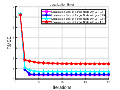
Figure 4: The convergence of proposed algorithm on the localization errors of the target node with different sensor node location errors under $10\log\left(\delta_{0}\right)=-30.$

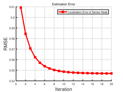
Figure 5: The convergence of proposed algorithm on the location refinement of the sensor node under sensor node location errors $\mu=0.5$ under $10\log\left(\delta_{0}\right)=-30.$

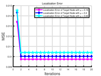
Figure 6: The convergence of proposed algorithm on the estimation of $\gamma$ under different sensor node location errors under $10\log\left(\mu\right)=-10$ and $10\log\left(\delta_{0}\right)=-30.$

VI-C Localization and Estimation Performances

In this subsection, we dig into the investigation of the localization error and channel estimation performances of the proposed JLCE algorithm alongside other algorithms through the exploration of various examples. This comparative investigation seeks to verify the effectiveness of the JLCE algorithm in the presence of uncertainties associated with sensor node positions, and provides valuable insights into its performance compared to other methodologies. In this analysis, we assume that the expectations of channel parameters are known for the all algorithms under consideration. It is crucial to highlight that sensor node location errors are taken into account for all algorithms studied, supporting a comprehensive evaluation of their robustness in real physical scenarios. Through this rigorous analysis, we aim to perceive the strengths and limitations of the JLCE algorithm, shedding light on its applicability and superiority in addressing challenges related to joint localization and channel estimation.

In Fig.7, we dig into the investigation of the localization performance of the proposed JLCE algorithm and other algorithms across varying reference noise powers $\delta_{0}$. The superior performance of the JLCE algorithm outperforms IRGLS algorithm, which can be attributed to the incorporation of prior information and the MMSE criterion. Moreover, the comparable accuracy achieved by JLCE and the ML-GMP algorithm stems from their common utilization of posterior distributions for both sensor nodes and the target node in the localization process. The numerical results unequivocally indicate the superior effectiveness of the proposed JLCE algorithm.

It is important to note that the benchmark BCRB is directly affected by noise power, comprising the reference noise power $\delta_{0}$ and the unknown distance $d_{i}$. As such, the rapid variations in reference noise power have a marginal impact on the benchmark, resulting in slight increases in the BCRB. In Fig.8, we present the estimation error of channel parameters, $\gamma$ achieved by the JLCE algorithm. The numerical results underscore the algorithm’s ability to attain accurate channel parameter estimations. Intuitively, as the reference noise power increases, the estimation errors also escalate, correlating with the observed rise in localization errors depicted in Fig.7. This is inherently correlated to the interplay between reference noise power and localization accuracy, indicating the intricate relationship between channel parameter estimation and noise model.

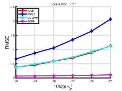
Figure 7: The localization errors of proposed algorithm JLCE and other algorithm with different reference noise power $\delta_{0}$ under $10\log\left(\mu\right)=-10$ and $10\log\left(\delta_{0}\right)=-30.$

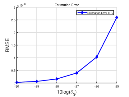
Figure 8: The estimation errors of the path loss exponent $\gamma$ of proposed algorithm JLCE with different reference noise power $\delta_{0}$ under $10\log\left(\mu\right)=-10.$

In Fig.9, we focus on the investigation of the localization performance of the proposed JLCE algorithm, along with other algorithms, across varying levels of sensor node uncertainties $\mu_{i}$. The numerical findings compellingly illustrate the adverse effects of sensor node location errors on localization performance of the target node. Moreover, the JLCE algorithm outperforms the IRGLS algorithm, showcasing its robustness in mitigating the negative impact of sensor node uncertainties. Furthermore, the comparable localization performances of the JLCE and ML-GMP algorithms align with expectations, as both leverage the MMSE criterion and incorporate prior distributions of sensor nodes and the target node in the localization process. These results are consistent with the findings reported in [36], highlighting the significant impact of sensor node location errors on the localization benchmark, a trend corroborated by the outcomes presented in Fig.9. The superiority of the proposed JLCE algorithm in navigating and minimizing the impact of sensor node uncertainties positions as a promising solution for robust localization in real-world scenarios.

To further investigate the impacts of distance over the estimation and localization performances, we enlarge the distances between the sensor nodes and target nodes by adding a coordinate offset $\boldsymbol{\Delta}_{s}$ to the sensor node locations.

In Fig.10 and Fig.11, the coordinate offset $\boldsymbol{\Delta}_{s}$ is set to be ${{\boldsymbol{\Delta}}_{s}}=\left[{50,50}\right]$ and the localization performances are investigated under different sensor node location errors $\mu$ and different different reference noise powers $\delta_{0}$. The simulation results both indicate the proposed algorithm can achieve superior performance than the other algorithms under greater distance-dependent noise. Comparing the results in Fig.9 and Fig.10, it is straightforward that greater distances bring negative impacts over the localization performances, which is validated in Fig.12. The ML-GMP algorithm is much more sensitive to the location offsets between the sensors and target node, which is resulted from the ML approximation step of ignoring the distance-dependent noise. The proposed algorithm merely are affected by the the location offsets due to the adoption of Taylor approximation over the complicated noise. These three results demonstrate that the proposed algorithm can achieve robust performances in worse noise environments.

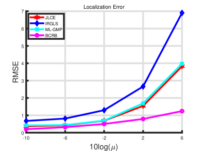
Figure 9: The localization errors of proposed algorithm JLCE and other algorithm with different sensor node uncertainties under $10\log\left(\delta_{0}\right)=-30$.

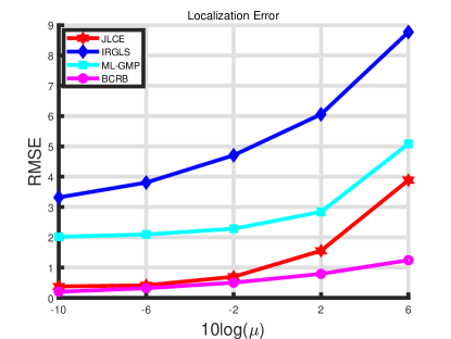
Figure 10: The localization errors of proposed algorithm JLCE and other algorithm with different sensor node uncertainties $\mu$ under $\boldsymbol{\Delta}_{s}=50$ and $10\log\left(\delta_{0}\right)=-30$.

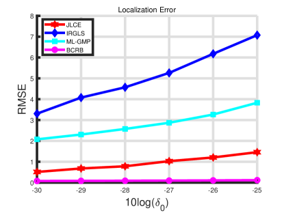
Figure 11: The localization errors of proposed algorithm JLCE and other algorithm with different reference noise power $\delta_{0}$ under $\boldsymbol{\Delta}_{s}=50$ and $10\log\left(\mu\right)=-10.$

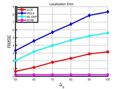
Figure 12: The localization errors of proposed algorithm JLCE and other algorithm with different sensor location offsets $\boldsymbol{\Delta}_{s}$ under $10\log\left(\delta_{0}\right)=-30$ under $10\log\left(\mu\right)=-10.$

VII Conclusion

The paper addresses a significant challenge in the field by exploring a joint problem involving localization and channel parameter estimation, taking into account both distance-dependent noise and uncertainties associated with sensor node positions. To tackle the inherent nonlinearity and non-convexity of the objective distribution function, a novel message passing approach is proposed. This method leverages a message passing algorithm to approximate the true posterior distribution and employs Taylor expansion to linearize the objective function. Subsequently, the target node location and channel parameters are estimated using either the MMSE or MAP techniques. Additionally, the paper digs into an investigation of the complexity and convergence characteristics of the proposed algorithm. The simulation results presented in the paper demonstrate the superior performance of the proposed algorithm in terms of channel estimation and localization accuracy across various illustrative examples. This innovative contribution not only addresses the intricacies of joint localization and channel parameter estimation but also presents the practical effectiveness of the proposed algorithm through rigorous simulations.

Appendix A

According to the equation (55), the submatrice ${{\boldsymbol{J}_{\boldsymbol{x}}}}$ can be given by

$$\begin{array}[]{*{20}{l}}{{\boldsymbol{J}_{\boldsymbol{x}}}=\underbrace{-{\mathbb{E}_{{\boldsymbol{r}},{\boldsymbol{\Theta}}}}\left[{\frac{{{\partial^{2}}\ln p\left({{\boldsymbol{r}}|{\boldsymbol{\Theta}}}\right)}}{{\partial{\boldsymbol{x}}\partial{{\boldsymbol{x}}^{T}}}}}\right]}_{{\boldsymbol{\cal I}^{{\boldsymbol{x}},{\boldsymbol{x}}}_{\rm{M}}}}\underbrace{-{\mathbb{E}_{\boldsymbol{\Theta}}}\left[{\frac{{{\partial^{2}}\ln p\left({\boldsymbol{x}}\right)}}{{\partial{\boldsymbol{x}}\partial{{\boldsymbol{x}}^{T}}}}}\right]}_{{\boldsymbol{\cal I}^{{\boldsymbol{x}},{\boldsymbol{x}}}_{\rm{P}}}},}\end{array}$$ (58)

By substituting the likelihood function $\eqref{likelihood}$ and prior distributions $\eqref{priorX}$ into (58), it yields

$$\boldsymbol{\cal I}_{\rm P}^{{\boldsymbol{x}},{\boldsymbol{x}}}=-{\mathbb{E}_{\boldsymbol{\Theta}}}\left[{\frac{{{\partial^{2}}\ln p\left({\boldsymbol{x}}\right)}}{{\partial{\boldsymbol{x}}\partial{{\boldsymbol{x}}^{T}}}}}\right]={{\boldsymbol{\Sigma}}^{-1}},$$ (59)

$$\begin{array}[]{l}\boldsymbol{\cal I}_{\rm M}^{{\boldsymbol{x}},{\boldsymbol{x}}}=-{\mathbb{E}_{{\boldsymbol{r}},{\boldsymbol{\Theta}}}}\left[{\frac{{{\partial^{2}}\ln p\left({{\boldsymbol{r}}|{\boldsymbol{\Theta}}}\right)}}{{\partial{\boldsymbol{x}}\partial{{\boldsymbol{x}}^{T}}}}}\right]={\mathbb{E}_{{\boldsymbol{r}},{\boldsymbol{\Theta}}}}\left[{\sum\limits_{i=1}^{N}{\frac{{{\partial^{2}}h\left({{\boldsymbol{x}},{{\boldsymbol{x}}_{i}}}\right)}}{{\partial{\boldsymbol{x}}\partial{{\boldsymbol{x}}^{T}}}}}}\right].\end{array}$$ (60)

where $h\left({{\boldsymbol{x}},{{\boldsymbol{x}}_{i}}}\right)=\sum\limits_{k=1}^{2}{h_{k}\left({{\boldsymbol{x}},{{\boldsymbol{x}}_{i}}}\right)}$ .

The above expectations involve nonlinear expectations with respect to the complicated distributions and it is extremely challenging to find the closed-form expressions. To obtain the approximation to the estimation performance benchmark, we apply second-order Taylor expansion to the nonlinear expectation ${\mathbb{E}_{p}}\left({{\mathcal{Z}}\left(\zeta\right)}\right)$ as follows

$${\mathbb{E}_{p}}\left({Z\left(\zeta\right)}\right) \approx{\mathbb{E}_{p}}\left({Z\left({{\mu_{\zeta}}}\right)}\right)+{\mathbb{E}_{p}}\left({{{\left.{\frac{{\partial Z}}{{\partial\zeta}}}\right|}_{\xi={\mu_{\zeta}}}}\left({\zeta-{\mu_{\zeta}}}\right)}\right)$$ (61)

$$+{\mathbb{E}_{p}}\left({\frac{1}{2}{{\left.{\frac{{{\partial^{2}}\mathcal{Z}}}{{\partial{\zeta^{2}}}}}\right|}_{\xi={\mu_{\zeta}}}}{{\left({\zeta-{\mu_{\zeta}}}\right)}^{2}}}\right)$$

$$\approx{\mathbb{E}_{p}}\left({\mathcal{Z}\left({{\mu_{\zeta}}}\right)}\right)+\frac{1}{2}{{\left.{\frac{{{\partial^{2}}\mathcal{Z}}}{{\partial{\zeta^{2}}}}}\right|}_{\xi={\mu_{\zeta}}}}{\delta_{\zeta}},$$

where ${\mathbb{E}_{p}}$ takes expectation with respect to $p\left(\zeta\right)$. ${\mu_{\zeta}}$ and $\delta_{\zeta}$ are the mean and variance of the distribution $p\left(\zeta\right)$. Meanwhile, the approximation holds with continuous and sufficiently differentiable ${{\mathcal{Z}}\left(\zeta\right)}$. Therefore, the expectation in (60) can be obtained via replacing the corresponding terms with tedious expectation approximations.

According to the equation (55), the submatrice ${{\boldsymbol{J}_{\boldsymbol{x},{{\boldsymbol{\Theta}}_{\backslash{\boldsymbol{x}}}}}}}$ can be given by

$${\boldsymbol{J}_{{\boldsymbol{x}},{{\boldsymbol{\Theta}}_{\backslash{\boldsymbol{x}}}}}}=\underbrace{-{\mathbb{E}_{{\boldsymbol{r}},{\boldsymbol{\Theta}}}}\left[{\frac{{{\partial^{2}}\ln p\left({{\boldsymbol{r}}|{\boldsymbol{\Theta}}}\right)}}{{\partial{\boldsymbol{x}}\partial{\boldsymbol{\Theta}}_{\backslash{\boldsymbol{x}}}^{T}}}}\right]}_{\boldsymbol{\cal I}_{\rm M}^{{\boldsymbol{x}},{{\boldsymbol{\Theta}}_{\backslash{\boldsymbol{x}}}}}},$$ (62)

which includes the following components

$${{\boldsymbol{J}}_{{\boldsymbol{x}},{{\boldsymbol{\Theta}}_{\backslash{\boldsymbol{x}}}}}}=\left[{\begin{array}[]{*{20}{c}}{{{\boldsymbol{J}}_{{\boldsymbol{x}},{{\boldsymbol{x}}_{1}}}}}&\ldots&{{{\boldsymbol{J}}_{{\boldsymbol{x}},{{\boldsymbol{x}}_{N}}}}}&{{{\boldsymbol{J}}_{{\boldsymbol{x}},\gamma}}}&{{{\boldsymbol{J}}_{{\boldsymbol{x}},{\Lambda_{0}}}}}\end{array}}\right].$$ (63)

Specifically, these components can be calculated respectively

$${{\boldsymbol{J}}_{{\boldsymbol{x}},{{\boldsymbol{x}}_{i}}}} =-{\mathbb{E}_{{\boldsymbol{r}},{\boldsymbol{\Theta}}}}\left({\frac{{\partial\ln p\left({{\boldsymbol{r}}\mid{\boldsymbol{\Theta}}}\right)}}{{\partial{\boldsymbol{x}}\partial{\boldsymbol{x}}_{i}^{T}}}}\right)$$ (64)

$$={\mathbb{E}_{\boldsymbol{\Theta}}}\left({\frac{{2{\Lambda_{0}}-{\gamma^{2}}d_{i}^{\gamma-2}}}{{2d_{i}^{\gamma}}}\frac{{\partial{d_{i}}}}{{\partial{\boldsymbol{x}}}}\frac{{\partial{d_{i}}}}{{\partial{\boldsymbol{x}}_{i}^{T}}}}\right),$$

$${{\boldsymbol{J}}_{{\boldsymbol{x}},\gamma}} =-{\mathbb{E}_{{\boldsymbol{r}},{\boldsymbol{\Theta}}}}\left({\frac{{\partial\ln p\left({{\bf{r}}\mid{\boldsymbol{\Theta}}}\right)}}{{\partial{\boldsymbol{x}}\partial{\gamma^{T}}}}}\right)$$ (65)

$$={\mathbb{E}_{\boldsymbol{\Theta}}}\left({\frac{1}{2}\frac{1}{{{d_{i}}}}\frac{{\partial{d_{i}}}}{{\partial{\boldsymbol{x}}}}-\frac{{d_{i}^{-1}-\gamma d_{i}^{-1}\ln{d_{i}}}}{2}\frac{{\partial{d_{i}}}}{{\partial{\boldsymbol{x}}}}}\right),$$

and

$${{\boldsymbol{J}}_{{\boldsymbol{x}},{\Lambda_{0}}}}=-{\mathbb{E}_{{\boldsymbol{r}},{\boldsymbol{\Theta}}}}\left({\frac{{\partial\ln p\left({{\boldsymbol{r}}\mid{\boldsymbol{\Theta}}}\right)}}{{\partial{\boldsymbol{x}}\partial\Lambda_{o}^{T}}}}\right)={\mathbb{E}_{\boldsymbol{\Theta}}}\left({\frac{{\gamma d_{i}^{-1}}}{{2{\Lambda_{0}}}}\frac{{\partial{d_{i}}}}{{\partial{\boldsymbol{x}}}}}\right),$$ (66)

where expectations can be obtained via the expectation approximations in (61).

According to the equation (55), the submatrice ${{\boldsymbol{J}}_{{{\boldsymbol{\Theta}}_{\backslash{\boldsymbol{x}}}},{{\boldsymbol{\Theta}}_{\backslash{\boldsymbol{x}}}}}}$ can be given by

$${{\boldsymbol{J}}_{{{\boldsymbol{\Theta}}_{\backslash{\boldsymbol{x}}}},{{\boldsymbol{\Theta}}_{\backslash{\boldsymbol{x}}}}}}=\underbrace{-{\mathbb{E}_{{\boldsymbol{r}},{\boldsymbol{\Theta}}}}\left[{\frac{{{\partial^{2}}\ln p\left({{\boldsymbol{r}}|{\boldsymbol{\Theta}}}\right)}}{{\partial{{\boldsymbol{\Theta}}_{\backslash{\boldsymbol{x}}}}\partial{\boldsymbol{\Theta}}_{\backslash{\boldsymbol{x}}}^{T}}}}\right]}_{\boldsymbol{\cal I}_{\rm{M}}^{{{\boldsymbol{\Theta}}_{\backslash{\boldsymbol{x}}}},{{\boldsymbol{\Theta}}_{\backslash{\boldsymbol{x}}}}}}\underbrace{-{\mathbb{E}_{\boldsymbol{\Theta}}}\left[{\frac{{{\partial^{2}}\ln p\left({\boldsymbol{x}}\right)}}{{\partial{{\boldsymbol{\Theta}}_{\backslash{\boldsymbol{x}}}}\partial{\boldsymbol{\Theta}}_{\backslash{\boldsymbol{x}}}^{T}}}}\right]}_{{\boldsymbol{\cal I}}_{\rm{P}}^{{{\boldsymbol{\Theta}}_{\backslash{\boldsymbol{x}}}},{{\boldsymbol{\Theta}}_{\backslash{\boldsymbol{x}}}}}}.$$ (67)

By substituting the likelihood function $\eqref{likelihood}$ and prior distributions $\eqref{messQgamma}$, $\eqref{messQLambda}$ and $\eqref{priorXi}$ into (58), it yields

$${{\boldsymbol{J}}_{{{\boldsymbol{x}}_{i}},{{\boldsymbol{x}}_{i}}}} =-{\mathbb{E}_{{\boldsymbol{r}},{\boldsymbol{\Theta}}}}\left({\frac{{{\partial^{2}}\ln p\left({{\boldsymbol{r}}|{\boldsymbol{\Theta}}}\right)}}{{\partial{{\boldsymbol{x}}_{i}}\partial{\boldsymbol{x}}_{i}^{T}}}}\right)-{\mathbb{E}_{{\boldsymbol{r}},{\boldsymbol{\Theta}}}}\left({\frac{{{\partial^{2}}\ln p\left({{{\boldsymbol{x}}_{i}}}\right)}}{{\partial{{\boldsymbol{x}}_{i}}\partial{\boldsymbol{x}}_{i}^{T}}}}\right)$$ (68)

$$={\mathbb{E}_{{\boldsymbol{r}},{\boldsymbol{\Theta}}}}\left[{\frac{{{\partial^{2}}h\left({{\boldsymbol{x}},{{\boldsymbol{x}}_{i}}}\right)}}{{\partial{\boldsymbol{x}}\partial{{\boldsymbol{x}}^{T}}}}}\right]+{\boldsymbol{\Sigma}}_{i}^{-1},$$

$${{\boldsymbol{J}}_{\gamma,\gamma}} =-{\mathbb{E}_{{\boldsymbol{r}},{\boldsymbol{\Theta}}}}\left({\frac{{{\partial^{2}}\ln p\left({{\boldsymbol{r}}|{\boldsymbol{\Theta}}}\right)}}{{\partial\gamma\partial{\gamma^{T}}}}}\right)-{\mathbb{E}_{\boldsymbol{\Theta}}}\left({\frac{{{\partial^{2}}\ln p\left(\gamma\right)}}{{\partial\gamma\partial{\gamma^{T}}}}}\right)$$ (69)

$$={\mathbb{E}_{\boldsymbol{\Theta}}}\left({\frac{1}{2}{{\left({\ln{d_{i}}}\right)}^{2}}}\right)+\delta_{\gamma}^{-1},$$

$${{\boldsymbol{J}}_{{\Lambda_{0}},{\Lambda_{0}}}} =-{\mathbb{E}_{{\boldsymbol{r}},{\boldsymbol{\Theta}}}}\left({\frac{{{\partial^{2}}\ln p\left({{\boldsymbol{r}}|{\boldsymbol{\Theta}}}\right)}}{{\partial{\Lambda_{0}}\partial\Lambda_{0}^{T}}}}\right)-{\mathbb{E}_{\boldsymbol{\Theta}}}\left({\frac{{{\partial^{2}}\ln p\left({{\Lambda_{0}}}\right)}}{{\partial{\Lambda_{0}}\partial\Lambda_{0}^{T}}}}\right)$$ (70)

$$={\mathbb{E}_{\boldsymbol{\Theta}}}\left({\left({0.5+b}\right)\Lambda_{0}^{-2}}\right).$$

References

- [1] M. S. Mekala, P. Rizwan, and M. S. Khan, “Computational intelligent sensor-rank consolidation approach for industrial Internet of things (IIoT),” IEEE Internet of Things Journal, vol. 10, no. 3, pp. 2121–2130, 2023.
- [2] R. S. Zakariyya, X. Wentau, Y. Zhang, R. Wang, Y. Huang, C. Duan, and Q. Zhang, “Joint DoA and CFO estimation scheme with received beam scanned leaky wave antenna for industrial Internet of things (IIoT) systems,” IEEE Internet of Things Journal, vol. 10, no. 15, pp. 13 686–13 696, 2023.
- [3] Y. Huo, X. Dong, and S. Beatty, “Cellular communications in ocean waves for maritime Internet of things,” IEEE Internet of Things Journal, vol. 7, no. 10, pp. 9965–9979, 2020.
- [4] L. Bai, R. Han, J. Liu, J. Choi, and W. Zhang, “Random access and detection performance of Internet of things for smart ocean,” IEEE Internet of Things Journal, vol. 7, no. 10, pp. 9858–9869, 2020.
- [5] M. A. Nazari, G. Seco-Granados, P. Johannisson, and H. Wymeersch, “Mmwave 6D radio localization with a snapshot observation from a single BS,” IEEE Transactions on Vehicular Technology, pp. 1–14, 2023.
- [6] G. Zhang, D. Zhang, Y. He, J. Chen, F. Zhou, and Y. Chen, “Multi-person passive WiFi indoor localization with intelligent reflecting surface,” IEEE Transactions on Wireless Communications, pp. 1–1, 2023.
- [7] J. Wu, S. Kim, and B. Shim, “Parametric sparse channel estimation for RIS-assisted Terahertz systems,” IEEE Transactions on Communications, vol. 71, no. 9, pp. 5503–5518, 2023.
- [8] Z. Chen, G. Chen, J. Tang, S. Zhang, D. K. So, O. A. Dobre, K.-K. Wong, and J. Chambers, “Reconfigurable-intelligent-surface-assisted B5G/6G wireless communications: Challenges, solution, and future opportunities,” IEEE Communications Magazine, vol. 61, no. 1, pp. 16–22, 2023.
- [9] Q. Zhu, M. Li, R. Liu, and Q. Liu, “Joint transceiver beamforming and reflecting design for active RIS-aided ISAC systems,” IEEE Transactions on Vehicular Technology, pp. 1–5, 2023.
- [10] R. Zhang, L. Cheng, S. Wang, Y. Lou, W. Wu, and D. W. K. Ng, “Tensor decomposition-based channel estimation for hybrid mmWave massive MIMO in high-mobility scenarios,” IEEE Transactions on Communications, vol. 70, no. 9, pp. 6325–6340, 2022.
- [11] M. Cui, Z. Wu, Y. Lu, X. Wei, and L. Dai, “Near-field MIMO communications for 6G: Fundamentals, challenges, potentials, and future directions,” IEEE Communications Magazine, vol. 61, no. 1, pp. 40–46, 2023.
- [12] Y. Lu, Z. Zhang, and L. Dai, “Hierarchical beam training for extremely large-scale MIMO: From far-field to near-field,” IEEE Transactions on Communications, pp. 1–1, 2023.
- [13] J. Du, M. Han, Y. Chen, L. Jin, and F. Gao, “Tensor-based joint channel estimation and symbol detection for time-varying mmWave massive MIMO systems,” IEEE Transactions on Signal Processing, vol. 69, pp. 6251–6266, 2021.
- [14] K. Ardah, S. Gherekhloo, A. L. F. de Almeida, and M. Haardt, “TRICE: A channel estimation framework for RIS-aided Millimeter-Wave MIMO systems,” IEEE Signal Processing Letters, vol. 28, pp. 513–517, 2021.
- [15] N. K. Kundu, S. P. Dash, M. R. Mckay, and R. K. Mallik, “Channel estimation and secret key rate analysis of MIMO Terahertz quantum key distribution,” IEEE Transactions on Communications, vol. 70, no. 5, pp. 3350–3363, 2022.
- [16] Y. Pan, C. Pan, S. Jin, and J. Wang, “RIS-aided near-field localization and channel estimation for the Terahertz system,” IEEE Journal of Selected Topics in Signal Processing, vol. 17, no. 4, pp. 878–892, 2023.
- [17] H. Chen, H. Sarieddeen, T. Ballal, H. Wymeersch, M.-S. Alouini, and T. Y. Al-Naffouri, “A tutorial on Terahertz-band localization for 6G communication systems,” IEEE Communications Surveys & Tutorials, vol. 24, no. 3, pp. 1780–1815, 2022.
- [18] R. C. Shit, S. Sharma, D. Puthal, P. James, B. Pradhan, A. v. Moorsel, A. Y. Zomaya, and R. Ranjan, “Ubiquitous localization (ubiloc): A survey and taxonomy on device free localization for smart world,” IEEE Communications Surveys & Tutorials, vol. 21, no. 4, pp. 3532–3564, 2019.
- [19] K. N. R. S. V. Prasad and V. K. Bhargava, “RSS localization under Gaussian distributed path loss exponent model,” IEEE Wireless Communications Letters, vol. 10, no. 1, pp. 111–115, 2021.
- [20] M. Golestanian and C. Poellabauer, “Variloc: Path loss exponent estimation and localization using multi-range beaconing,” IEEE Communications Letters, vol. 23, no. 4, pp. 724–727, 2019.
- [21] Y. Zou and H. Liu, “RSS-based target localization with unknown model parameters and sensor position errors,” IEEE Transactions on Vehicular Technology, vol. 70, no. 7, pp. 6969–6982, 2021.
- [22] X. Yang, C.-K. Wen, Y. Han, S. Jin, and A. L. Swindlehurst, “Soft channel estimation and localization for millimeter wave systems with multiple receivers,” IEEE Transactions on Signal Processing, vol. 70, pp. 4897–4911, 2022.
- [23] C. Wei, K. Xu, Z. Shen, X. Xia, C. Li, W. Xie, D. Zhang, and H. Liang, “Fingerprint-based localization and channel estimation integration for cell-free massive MIMO IoT systems,” IEEE Internet of Things Journal, vol. 9, no. 24, pp. 25 237–25 252, 2022.
- [24] J. Hong, J. Rodríguez-Piñeiro, X. Yin, and Z. Yu, “Joint channel parameter estimation and scatterers localization,” IEEE Transactions on Wireless Communications, vol. 22, no. 5, pp. 3324–3340, 2023.
- [25] T. Kazaz, G. J. M. Janssen, J. Romme, and A.-J. van der Veen, “Delay estimation for ranging and localization using multiband channel state information,” IEEE Transactions on Wireless Communications, vol. 21, no. 4, pp. 2591–2607, 2022.
- [26] B. Zhou, J. Wen, H. Chen, and V. K. N. Lau, “The effect of multipath propagation on performance limit of mmWave MIMO-based position, orientation and channel estimation,” IEEE Transactions on Vehicular Technology, vol. 71, no. 4, pp. 3851–3867, 2022.
- [27] X. Zheng, A. Liu, and V. Lau, “Joint channel and location estimation of massive MIMO system with phase noise,” IEEE Transactions on Signal Processing, vol. 68, pp. 2598–2612, 2020.
- [28] F. Wen, P. Liu, H. Wei, Y. Zhang, and R. C. Qiu, “Joint azimuth, elevation, and delay estimation for 3-D indoor localization,” IEEE Transactions on Vehicular Technology, vol. 67, no. 5, pp. 4248–4261, 2018.
- [29] Y. Liang and Y. Jia, “Constrained optimal placements of heterogeneous range/bearing/RSS sensor networks for source localization with distance-dependent noise,” IEEE Geoscience and Remote Sensing Letters, vol. 13, no. 11, pp. 1611–1615, 2016.
- [30] W. Wang, P. Bai, Y. Zhou, X. Liang, and Y. Wang, “Optimal configuration analysis of AOA localization and optimal heading angles generation method for UAV swarms,” IEEE Access, vol. 7, pp. 70 117–70 129, 2019.
- [31] W. Yan, X. Fang, and J. Li, “Formation optimization for AUV localization with range-dependent measurements noise,” IEEE Communications Letters, vol. 18, no. 9, pp. 1579–1582, 2014.
- [32] B. Huang, L. Xie, and Z. Yang, “TDOA-based source localization with distance-dependent noises,” IEEE Transactions on Wireless Communications, vol. 14, no. 1, pp. 468–480, 2015.
- [33] Y. Li, S. Ma, and G. Yang, “Robust localization with distance-dependent noise and sensor location uncertainty,” IEEE Wireless Communications Letters, vol. 10, no. 9, pp. 1876–1880, 2021.
- [34] Y. Li, L. Liu, W. Yu, Y. Wang, and X. Guan, “Noncooperative mobile target tracking using multiple AUVs in anchor-free environments,” IEEE Internet of Things Journal, vol. 7, no. 10, pp. 9819–9833, 2020.
- [35] Y. Li, B. Li, W. Yu, S. Zhu, and X. Guan, “Cooperative localization based multi-AUV trajectory planning for target approaching in anchor-free environments,” IEEE Transactions on Vehicular Technology, vol. 71, no. 3, pp. 3092–3107, 2022.
- [36] Y. Li, S. Ma, G. Yang, and K. Wong, “Robust localization for mixed LOS/NLOS environments with anchor uncertainties,” IEEE Transactions on Communications, vol. 68, no. 7, pp. 4507–4521, 2020.
- [37] Y. Li, S. Ma, G. Yang, and K.-K. Wong, “Secure localization and velocity estimation in mobile IoT networks with malicious attacks,” IEEE Internet of Things Journal, vol. 8, no. 8, pp. 6878–6892, 2021.
- [38] N. Nasios and A. G. Bors, “Variational learning for Gaussian mixture models,” IEEE Trans. Syst. Man Cybern. Syst., Part B (Cybernetics), vol. 36, no. 4, pp. 849–862, 2006.
- [39] B. Li, N. Wu, Y.-C. Wu, and Y. Li, “Convergence-guaranteed parametric Bayesian distributed cooperative localization,” IEEE Transactions on Wireless Communications, vol. 21, no. 10, pp. 8179–8192, 2022.
- [40] J. Winn and C. Bishop, “Variational message passing,” JOURNAL OF MACHINE LEARNING RESEARCH, vol. 6, pp. 661–694, APR 2005.