Noise-induced oscillations
for the mean-field Dissipative Contact Process

Paolo DaiΒ Pra, Elisa Marini
Abstract

We study a dissipative version of the contact process, with mean-field interaction, which admits a simple epidemiological interpretation. The propagation of chaos and the corresponding normal fluctuations reveal that the noise present in the finite-size system induces oscillations with a nearly deterministic period and a randomly varying amplitude. This is reminiscent of the emergence of pandemic waves in real epidemics.

1 Introduction

The contact process is the microscopic counterpart of one of the most basic epidemiological models, the SIS model. Suppose the individuals of a population are placed at the vertices of a graph $(V,E)$; the individual at the vertex $i\in V$ can be either susceptible ($x_{i}=0$) or non susceptible ($x_{i}=1$). The configuration $x=(x_{i})_{i\in V}$ evolves as a continuous time Markov chain with the following rates:

  • β€’

    each non susceptible individual becomes susceptible with rate 111;

  • β€’

    each susceptible individual becomes non susceptible with a rate equal to a given constant $\lambda$ times the fraction of non susceptible neighbors.

This definition suffices in finite graphs, while further care is needed in countable graphs (see [4]). In finite graphs the chain is absorbed in the null state ($x_{i}\equiv 0$) in finite time (we say that the epidemics dies out). The time to absorption could however vary from a fast absorption (at most polynomial in $|V|$) to a slow absorption (exponential in $|V|$). For many (sequences of) graphs the transition from fast to slow absorption occurs as the infection constant $\lambda$ crosses a critical value $\overline{\lambda}$. The simplest nontrivial example is the case in which $(V,E)$ is the complete graph of $N$ vertices: $V=\{1,2,\ldots,N\}$, $E=V\times V$. The study of this model reduces to the analysis of the one-dimensional Markov process

$$m_{N}:=\frac{1}{N}\sum_{i=1}^{N}x_{i},$$

and the critical infection constant is $\overline{\lambda}=1$. Infinite countable graphs require a more detailed analysis, leading to results in several directions, including ergodicity, convergence, local and global survival of the epidemics; such rich behavior could imply the existence of more than one critical value for the infection constant.

In this paper we introduce a modification of the contact process. The state $x_{i}$ of each individual takes values in the interval $[0,1]$, and is interpreted as her viral load; we say that an individual is susceptible if $x_{i}=0$. The dynamics goes as follows:

  • β€’

    each non susceptible individual becomes susceptible with rate $r>0$;

  • β€’

    each susceptible individual becomes non susceptible with a rate equal to $\lambda>0$ times the arithmetic mean of the viral loads of her neighbors, and her viral load jumps to the value $1$;

  • β€’

    between jumps, the viral load decays exponentially with rate $\alpha>0$.

Note that the model is overparametrized, as we could rescale the time to have $r=1$. We keep however all parameters as they have a useful interpretation: $r^{-1}$ is the time scale at which infected (i.e. non susceptible) individuals lose their immunity, while $\alpha^{-1}$ is the time scale at which infected individuals remain contagious. In many real epidemics $\alpha^{-1}\ll r^{-1}$: for a relatively long time non susceptible individuals are immune, and do not contribute to the propagation of the disease. Note that many of the useful mathematical properties of the contact process are lost; for instance, monotonicity breaks due to the presence of immune individuals that block contagion.

In this paper we study this modified contact process, that we call dissipative, on the complete graph. Unlike the corresponding classical contact process, the dissipative version does not admit a finite dimensional reduction: any finite-dimensional functional of the empirical measure is non Markovian for large $N$. We particularly deal with the thermodynamic limit of the process ($N\rightarrow+\infty$), and we obtain a law of large numbers (propagation of chaos) and a central limit theorem. Despite the lack of finite dimensional reduction, both the limit process corresponding to the law of large numbers and the limit fluctuation process corresponding to the central limit theorem are two-dimensional. Under suitable conditions on the parameters, including the case $\alpha^{-1}\ll r^{-1}$, the limit process has a unique stable fixed point, which is approached by damped oscillations. The limit fluctuation process reveals, via a Fourier analysis, that noise induces persistent oscillations, despite of the damping exhibited by the limit process. The nature of these oscillations is then investigated by letting the parameters $\alpha$ and $\lambda$ to diverge (slowly) with $N$: if properly rescaled, the dynamics of the fraction of non susceptible individuals and of the mean viral load converges to a harmonic oscillator affected by noise. In their epidemiological interpretation these results suggest that pandemic waves are induced by finite-size effects, allowing the random noise to excite frequencies close to a characteristic value. The resulting motion is however not strictly periodic: though the period is nearly constant, the amplitude of each oscillation is significantly affected by noise, in agreement with what observed in real epidemics.

This paper is organized as follows. Section 2 deals with the derivation of the dynamics of a representative individual in the limit as $N\rightarrow+\infty$. Detailed properties of this limit dynamics are studied in Section 3. In Section 4 we study the dynamics of normal fluctuations around the limit dynamics. In Section 5 we scale with $N$ the parameters $\alpha$ and $\lambda$ of the model, and study the corresponding limit dynamics. Unless otherwise stated, all proof are collected in Section 6.

2 Microscopic dynamics and propagation of chaos

We consider a population of $N$ individuals whose states $(x_{i})_{i=1}^{N}$ take values in $[0,1]$. The microscopic dynamics of the system is sketched in Figure 1.

$\displaystyle 0$ $\displaystyle 1$ $\displaystyle e^{-\alpha t}$ $\displaystyle\frac{\lambda}{N}\sum_{j=1}^{N}x_{j}$ $\displaystyle r$ $\displaystyle\alpha$
Figure 1: An individual $i$ who is initially susceptible ($x_{i}=0$), can become infectious with rate $\frac{\lambda}{N}\sum_{j=1}^{N}x_{j}$ (mean-field interaction). When this happens, her viral load $x_{i}$ jumps to the value $1$. When infectious, individual $i$ can recover with rate $r$ and, in this case, she becomes immediately susceptible again. In the meantime, the viral load of the individual decreases deterministically in time with rate $\alpha$. Notice that this dynamics is invariant under permutations of the particles. This model is a piecewise deterministic Markov process, as the $x_{i}$s have a deterministic continuous dynamics with discontinuities determined by random jump events.

We define $m_{N}(t)$ and $v_{N}(t)$ to be the average number of infected individuals and the average viral load of the $N$-particle system at time $t$ respectively, namely,

$$m_{N}(t)\coloneqq\frac{1}{N}\sum_{i=1}^{N}{\bf{1}}_{\{x_{i}(t)>0\}}=\int_{0}^{1}{\bf{1}}_{\{y>0\}}\rho^{N}_{t}(dy)$$ (1)

and

$$v_{N}(t)\coloneqq\frac{1}{N}\sum_{i=1}^{N}x_{i}(t)=\int_{0}^{1}y\rho^{N}_{t}(dy)$$ (2)

where $\rho^{N}_{t}$ is the empirical measure of $\left(x_{i}\right)_{i=1}^{N}$ at time $t$, i.e., the measure-valued process

$$\rho^{N}_{t}\coloneqq\frac{1}{N}\sum_{i=1}^{N}\delta_{x_{i}(t)}$$ (3)

The state $\mathcal{X}^{N}\coloneqq\left(x_{i}\right)_{i=1}^{N}$, taking values on $[0,1]^{N}$, is a Markov process whose infinitesimal generator is the closure of the operator $\mathcal{L}^{N}$ acting on continuously differentiable functions $\phi\in C^{1}\left([0,1]^{N}\right)$ as

$$\begin{split}\mathcal{L}^{N}\phi\left(\mathcal{X}^{N}\right)&=\sum_{k=1}^{N}-\alpha x_{k}\partial_{x_{k}}\phi\left(\mathcal{X}^{N}\right)\\ &+\sum_{k=1}^{N}{\bf{1}}_{\{x_{k}(t)=0\}}\lambda v_{N}\left[\phi\left(\mathcal{X}^{N,\uparrow,k}\right)-\phi\left(\mathcal{X}^{N}\right)\right]\\ &+\sum_{k=1}^{N}{\bf{1}}_{\{x_{k}(t)>0\}}r\left[\phi\left(\mathcal{X}^{N,\downarrow,k}\right)-\phi\left(\mathcal{X}^{N}\right)\right]\end{split}$$ (4)

where $\mathcal{X}^{N,\uparrow,k}$ denotes a state equal to $\mathcal{X}^{N}$, except for the $k$-th coordinate, which is $1$, and $\mathcal{X}^{N,\downarrow,k}$ denotes a state equal to $\mathcal{X}^{N}$, except for the $k$-th coordinate, which is 00.

Equivalently, the state $x_{i}(t)$ of each individual evolves according to

xi​(t)=xi​(0)βˆ’βˆ«0tα​xi​(s)​𝑑s+∫[0,t]Γ—[0,+∞)𝟏[0,𝟏{xi​(sβˆ’)=0}​λ​vN​(sβˆ’)]​(u)​Ni↑​(d​s,d​u)βˆ’βˆ«[0,t]Γ—[0,+∞)xi​(sβˆ’)β€‹πŸ[0,𝟏{xi​(sβˆ’)>0}​(sβˆ’)​r]​(u)​Ni↓​(d​s,d​u)subscriptπ‘₯𝑖𝑑subscriptπ‘₯𝑖0superscriptsubscript0𝑑𝛼subscriptπ‘₯𝑖𝑠differential-d𝑠subscript0𝑑0subscript10subscript1subscriptπ‘₯𝑖superscript𝑠0πœ†subscript𝑣𝑁superscript𝑠𝑒subscriptsuperscript𝑁↑𝑖𝑑𝑠𝑑𝑒subscript0𝑑0subscriptπ‘₯𝑖superscript𝑠subscript10subscript1subscriptπ‘₯𝑖superscript𝑠0superscriptπ‘ π‘Ÿπ‘’subscriptsuperscript𝑁↓𝑖𝑑𝑠𝑑𝑒\begin{split}x_{i}(t)&=x_{i}(0)-\int_{0}^{t}\alpha x_{i}(s)ds+\int_{[0,t]\times[0,+\infty)}\boldsymbol{1}_{[0,{\bf{1}}_{\{x_{i}(s^{-})=0\}}\lambda v_{N}(s^{-})]}(u)N^{\uparrow}_{i}(ds,du)\\ &-\int_{[0,t]\times[0,+\infty)}x_{i}(s^{-})\boldsymbol{1}_{[0,{\bf{1}}_{\{x_{i}(s^{-})>0\}}(s^{-})r]}(u)N^{\downarrow}_{i}(ds,du)\end{split} (5)

Here $(N^{\uparrow}_{i})_{i=1}^{N}$ and $(N^{\downarrow}_{i})_{i=1}^{N}$ are families of independent Poisson random measures on $[0,+\infty)\times[0,+\infty)$ with intensity measure the Lebesgue measure $dt\times du$. Moreover, $N^{\uparrow}_{i}$ and $N^{\downarrow}_{j}$ are independent for all $i,j\in\left\{1,\dots,N\right\}$. Notice that integrating over $[0,t]$ makes the processes $x_{i}$ cΓ dlΓ g. Also, here $f(t^{-})\coloneqq\lim_{s\to t^{-}}f(s)$ is standard notation for the left limit of a function $f$ at $t$. Strong existence and uniqueness for system (5) can be proven as in [3].

We will prove that the evolution of a representative component in the limit as $N\rightarrow+\infty$ is given by the stochastic differential equation

$$\begin{split}\bar{x}(t)&=\bar{x}(0)-\int_{0}^{t}\alpha\bar{x}(s)ds+\int_{[0,t]\times[0,+\infty)}\boldsymbol{1}_{[0,{\bf{1}}_{\{\bar{x}(s^{-})=0\}}\lambda v(s^{-})]}(u)N^{\uparrow}(ds,du)\\ &-\int_{[0,t]\times[0,+\infty)}\bar{x}(s^{-})\boldsymbol{1}_{[0,{\bf{1}}_{\{\bar{x}(s^{-})>0\}}r]}(u)N^{\downarrow}(ds,du)\end{split}$$ (6)

where $N^{\uparrow}$ and $N^{\downarrow}$ are independent Poisson random measures on $[0,+\infty)\times[0,+\infty)$, both having intensity measure $dt\times du$, and $v(t)\coloneqq\int_{[0,+\infty)}u\rho_{\bar{x}(t)}(du)$ is the first moment of the law $\rho_{\bar{x}}$ of the variable $\bar{x}$ at time $t$.

Notice that Eq. (6) is a nonlinear, also called McKean-Vlasov, SDE, as the law of its solution appears as an argument of its coefficients through its first moment $v$. Existence and pathwise uniqueness of a strong solution to system (6) follow straightforwardly from [1] and [3].

Theorem 2.1 (Propagation of chaos).

Suppose $\left(x_{i}(0)\right)_{i=1}^{N}$ are independent identically distributed random variables with values in $[0,1]$ and law $\mu_{0}$. Denote by $(\left(x_{i}(t)\right)_{t\geq 0})_{i=1}^{N}$ the corresponding solution to system (5). Also, consider $N$ independent copies of the solution to Eq. (6), $(\left(\bar{x}_{i}(t)\right)_{t\geq 0})_{i=1}^{N}$, with the same Poisson random measures $N^{\uparrow}_{i}$, $N^{\downarrow}_{i}$, $i=1,\dots,N$ and the same initial conditions of system (5).

Then, for all $i=1,\dots,N$ and for all $T>0$,

$${\mathbb{E}}\left[\sup_{t\in[0,T]}\left\{\left|x_{i}(t)-\bar{x}_{i}(t)\right|+\left|{\bf{1}}_{\{x_{i}(t)>0\}}-{\bf{1}}_{\{\bar{x}_{i}(t)>0\}}\right|\right\}\right]\leq\frac{A_{T}}{\sqrt{N}}$$ (7)

where

$$A_{T}=\lambda Te^{(\alpha+3\lambda+2r)T}.$$ (8)

The proof of Theorem 2.1 is a standard application of coupling arguments and Gromwall Lemma. We however include it in this paper since the specific form of the constant $A_{T}$ will be useful in Section 5.

Theorem 2.1, together with the fact that the i.i.d. processes $\bar{x}_{i}$ satisfy a standard Law of Large Numbers, implies the following result.

Corollary 2.2.

For every $T>0$

$$\begin{split}{\mathbb{E}}\left[\sup_{t\in[0,T]}\left|m_{N}(t)-{\mathbb{P}}\left[\bar{x}(t)>0\right]\right|\right]&\leq\frac{B_{T}}{\sqrt{N}}\qquad\qquad{\mathbb{E}}\left[\sup_{t\in[0,T]}\left|v_{N}(t)-{\mathbb{E}}\left[\bar{x}(t)\right]\right|\right]\leq\frac{B_{T}}{\sqrt{N}}\end{split}$$ (9)

where

$$B_{T}=\left[\lambda T+1+K_{1}\sqrt{T(\lambda+r)}\right]e^{(\alpha+3\lambda+2r)T},$$ (10)

and $K_{1}$ is the best constant in the Burkholder-Davis-Gundy inequality in $L^{1}$. Moreover, defining

$$v_{N,2}(t):=\frac{1}{N}\sum_{i=1}^{N}x_{i}^{2}(t),$$ (11)

we have

$${\mathbb{E}}\left[\sup_{t\in[0,T]}\left|v_{N,2}(t)-{\mathbb{E}}\left[\bar{x}^{2}(t)\right]\right|\right]\leq\frac{C_{T}}{\sqrt{N}},$$ (12)

where

$$C_{T}=2A_{T}+(1+\lambda T+K_{1}(3\sqrt{\lambda}+\sqrt{r})\sqrt{T})e^{(2\alpha+r)T}.$$ (13)

3 Macroscopic dynamics of aggregated variables

3.1 Evolution of the mean values

By taking the expectation in Eq. (6), it is easy to obtain the evolution equations for

$$m(t)\coloneqq{\mathbb{P}}\left[\bar{x}(t)>0\right]$$ (14)

and

$$v(t)\coloneqq{\mathbb{E}}\left[\bar{x}(t)\right],$$ (15)

which are given by

$$\begin{split}&\dot{m}(t)=\lambda(1-m(t))v(t)-rm(t)\\ &\dot{v}(t)=-\alpha v(t)+\lambda(1-m(t))v(t)-rv(t).\end{split}$$ (16)

It is easily seen that $(0,0)$ is always a fixed point for (16). Under the condition $\frac{r+\alpha}{\lambda}<1$ a nonzero fixed point exists:

$$\left(m^{\ast},v^{\ast}\right)\coloneqq\left(1-\frac{r+\alpha}{\lambda},\frac{r}{r+\alpha}\left(1-\frac{r+\alpha}{\lambda}\right)\right)$$ (17)

Linear stability for these fixed points is readily checked with the Jacobian matrix of the vector field in (16):

$$J(m,v)=\begin{bmatrix}-\lambda v-r&\lambda(1-m)\\ -\lambda v&\lambda(1-m)-(r+\alpha)\end{bmatrix}$$ (18)

As

$$J(0,0)=\begin{bmatrix}-r&\lambda\\ 0&\lambda-(r+\alpha)\end{bmatrix}$$ (19)

we see that the origin is linearly stable for $\frac{r+\alpha}{\lambda}>1$. Its asymptotic global stability for $\frac{r+\alpha}{\lambda}\geq 1$ follows from the absence of limit cycles, that can be proved by employing Dulac’s criterion: defining $g(m,v)\coloneqq v^{-1}$, it holds

$$div\left(g(m,v)\begin{bmatrix}\dot{m}\\ \dot{v}\end{bmatrix}\right)=-\lambda-\frac{r}{v}<0\quad\forall\,0\leq m\leq 1,\,0<v\leq 1.$$ (20)

Under the condition $\frac{r+\alpha}{\lambda}<1$, the Jacobian matrix

$$J(m^{\ast},v^{\ast})=\begin{bmatrix}-\frac{r\lambda}{r+\alpha}&r+\alpha\\ -\frac{r\lambda}{r+\alpha}\left(1-\frac{r+\alpha}{\lambda}\right)&0\end{bmatrix}$$ (21)

has eigenvalues

$$\lambda_{\pm}=\frac{1}{2}\left(-\frac{r\lambda}{r+\alpha}\pm\frac{r\lambda}{r+\alpha}\sqrt{1-\frac{4(r+\alpha)^{2}}{r\lambda}\left(1-\frac{r+\alpha}{\lambda}\right)}\right)$$ (22)

which have negative real part. Thus the fixed point $(m^{\ast},v^{\ast})$ is linearly stable whenever it exists. Its global stability follows form the above Dulac’s criterion. Note also that the eigenvalues $\lambda_{\pm}$ are real and negative when

$$\frac{4(r+\alpha)^{2}}{r\lambda}\left(1-\frac{r+\alpha}{\lambda}\right)\leq 1$$

which happens when

$$\lambda\leq\lambda_{-}\coloneqq\frac{2(r+\alpha)^{2}}{r}\left(1-\sqrt{\frac{\alpha}{r+\alpha}}\right)\text{ or }\lambda\geq\lambda_{+}\coloneqq\frac{2(r+\alpha)^{2}}{r}\left(1+\sqrt{\frac{\alpha}{r+\alpha}}\right)$$ (23)

and are complex and conjugate with negative real part when

$$\lambda_{-}<\lambda<\lambda_{+}$$

Notice that $r+\alpha<\lambda_{-}$. Thus, $(m^{\ast},v^{\ast})$ is a stable node when $r+\alpha<\lambda\leq\lambda_{-}$ or $\lambda\geq\lambda_{+}$ and a stable spiral when $\lambda_{-}<\lambda<\lambda_{+}$.

Remark 3.1.

In the Contact process without dissipation there is correspondence between the Markovianity of the one dimensional process $m_{N}(t)$ and the fact that its limit is causal, i.e. solves a well posed one dimensional Cauchy problem. In the dissipative Contact process, the limit process $(m(t),v(t))$ is causal, but its pre-limit counterpart is not Markovian. Indeed, the presence of the term

$$\int_{[0,t]\times[0,+\infty)}x_{i}(s^{-})\boldsymbol{1}_{[0,{\bf{1}}_{\{x_{i}(s^{-})>0\}}r]}(u)N^{\downarrow}_{i}(ds,du)$$

in the evolution of $x_{i}$, produces for $v_{N}$ a martingale with a quadratic variation containing a term proportional to

$$\frac{1}{N}\sum_{i=1}^{N}\int_{0}^{t}x_{i}^{2}(s)ds,$$

which is not a function of $(m_{N},v_{N})$. The contribution of this term, however, vanishes in the limit as $N\rightarrow+\infty$. It can be shown that the dissipative Contact process does not admit any finite dimensional reduction, in the sense that no finite dimensional statistics of the microscopic variables has the Markov property for all $N$.

3.2 The distribution of $\bar{x}$

Our aim in this subsection is to determine the asymptotic distribution of the viral load. We denote by $(\rho^{\mu_{0}}_{\bar{x}(t)})_{t\geq 0}$ the flow of the distributions of $\bar{x}$, with the initial condition $\bar{x}(0)\sim\mu_{0}$. Moreover, let $(m(t),v(t))$ be the solution of (16) with initial conditions $m(0)={\mathbb{P}}(\bar{x}(0)>0)$, $v(0)={\mathbb{E}}[\bar{x}(0)]$.

Theorem 3.2.

For any initial distribution $\mu_{0}$ on $[0,1]$, the distribution at time $t$ of the limit process $\bar{x}$ when the initial distribution is $\bar{x}(0)\sim\mu_{0}$ is given by

$$\begin{split}\rho_{\bar{x}(t)}^{\mu_{0}}(d\bar{x})&=\int_{0}^{1}\rho^{\bar{x}_{0}}_{\bar{x}(t)}(d\bar{x})\mu_{0}(d\bar{x}_{0})\end{split}$$ (24)

with

$$\begin{split}&\rho^{\bar{x}_{0}}_{\bar{x}(t)}(d\bar{x})\coloneqq e^{-rt}\boldsymbol{1}_{\bar{x}_{0}>0}\delta_{\bar{x}_{0}e^{-\alpha t}}(d\bar{x})+g_{t}(\bar{x})\boldsymbol{1}_{(e^{-\alpha t},1]}(\bar{x})d\bar{x}+k(t)\delta_{0}(d\bar{x})\end{split}$$ (25)

the marginal law at time $t$ of the limit $\bar{x}$ process started at the deterministic initial condition $\bar{x}(0)=\bar{x}_{0}\in[0,1]$, with

$$g_{t}(\bar{x})\coloneqq\frac{\lambda\,k\left(t+\frac{1}{\alpha}\ln{\left(\bar{x}\right)}\right)v\left(t+\frac{1}{\alpha}\ln{\left(\bar{x}\right)}\right)}{\alpha}\bar{x}^{\frac{r-\alpha}{\alpha}}$$ (26)

and $k(t)$ being the solution to

$$\begin{cases}\dot{k}(t)+\lambda v(t)k(t)=r\left(1-k(t)\right)\\ k(0)=\boldsymbol{1}_{\{\bar{x}_{0}=0\}}\end{cases}$$ (27)

Besides $\delta_{0}$, the unique stationary distribution is given by

$$\begin{split}\rho^{\ast}(d\bar{x})&=\frac{\lambda\,r}{\alpha}\frac{v^{\ast}}{\lambda\,v^{\ast}+r}\bar{x}^{\frac{r-\alpha}{\alpha}}d\bar{x}+k^{\ast}\delta_{0}(d\bar{x})\\ &=\frac{r}{\alpha}\left(1-\frac{r+\alpha}{\lambda}\right)\bar{x}^{\frac{r-\alpha}{\alpha}}d\bar{x}+\frac{r+\alpha}{\lambda}\delta_{0}(d\bar{x})\end{split}$$ (28)

where $k^{\ast}=\lim_{t\to+\infty}k(t)=\frac{r}{\lambda\,v^{\ast}+r}$ is the stationary solution to Eq. (27). Moreover, $\rho^{\ast}$ is the limit distribution (as $t\rightarrow+\infty$) for all initial distributions $\mu_{0}$ different from $\delta_{0}$.

Remark 3.3.

We give a heuristic interpretation of (25). The first summand arises as, starting from $\bar{x}_{0}>0$, the limit process $\bar{x}$ evolves deterministically and decreases exponentially fast to zero until a jump to $\bar{x}=0$ occurs. This happens with rate $r$, so the probability that, at any time $t>0$ and starting from $\bar{x}_{0}>0$, the process $\bar{x}$ has not jumped to zero yet is $e^{-rt}$. As soon as $\bar{x}$ undergoes a jump to zero, the initial condition $\bar{x}_{0}$ is forgotten.

This is when the second and the third summands come into play. The second summand constitutes the absolutely continuous part of $\rho^{\bar{x}_{0}}_{\bar{x}(t)}$. It is turned on as $\bar{x}$, after having reached zero for the first time, jumps for the first time to $1$. Indeed, the only way $\boldsymbol{1}_{(e^{-\alpha t},1]}(\bar{x}(t))$ can be different from zero is when $\bar{x}$ decays deterministically from $\bar{x}_{0}$ for a time $s\leq t$, then jumps to zero and then to $1$ before time $t$, and from $1$ resumes a deterministic decay (possibly with other extra jumps to zero and $1$) so that, by time $t$, $\bar{x}(t)\in(e^{-\alpha t},1]$. In fact, if $\bar{x}$ underwent only a deterministic decay from $\bar{x}_{0}$ at time 00 to time $t$, we could only find $\bar{x}(t)\leq e^{-\alpha t}$.

The last summand accounts for the fact that the process can jump to zero and stay in zero for some time.

4 The fluctuation process and its Gaussian limit

We now consider the fluctuation process

$$\begin{split}X^{N}(t)\coloneqq\begin{bmatrix}\xi^{N}(t)\\ \eta^{N}(t)\end{bmatrix}\coloneqq\begin{bmatrix}\sqrt{N}\left(m_{N}(t)-m(t)\right)\\ \sqrt{N}\left(v_{N}(t)-v(t)\right)\end{bmatrix}\end{split}$$ (29)

As observed in Remark 3.1, this process is not Markovian. However, we prove a Central Limit Theorem that implies its convergence to a Gauss-Markov process.

Theorem 4.1 (Diffusion approximation of the fluctuation process).

As in Theorem 2.1 we assume that $(x_{i}(0))_{i=1}^{N}$ are independent identically distributed random variables with values in $[0,1]$ and law $\mu_{0}$. In particular, $X^{N}(0)$ converges in distribution to a Gaussian random variable $X_{0}$. Then $X^{N}$ converges in distribution, in any interval $[0,T]$, to the solution $X(t)=\left[\xi(t),\,\eta(t)\right]^{T}$ to the following linear stochastic differential equation

$$\begin{split}&dX(t)=F(t)X(t)dt+\Sigma(t)dW(t)\\ &X(0)=X_{0}\end{split}$$ (30)

where

$$F(t)\coloneqq\begin{bmatrix}-\left(\lambda v(t)+r\right)&\lambda(1-m(t))\\ -\lambda v(t)&\lambda\left(1-m(t)\right)-r-\alpha\end{bmatrix}$$ (31)

is the drift matrix, $W(t)$ is a two-dimensional standard Brownian motion and the diffusion matrix $\Sigma(t)$ is the (unique, symmetric) square root of the matrix $A(t)$ given by

$$A(t)=\Sigma(t)\Sigma^{T}(t)=\begin{bmatrix}\lambda\left(1-m(t)\right)v(t)+rm(t)&\lambda\left(1-m(t)\right)v(t)+r\lambda v(t)\\ \lambda\left(1-m(t)\right)v(t)+rv(t)&\lambda\left(1-m(t)\right)v(t)+r{\mathbb{E}}\left[\bar{x}^{2}(t)\right]\end{bmatrix}$$ (32)

where $\bar{x}(t)$ is the limit process defined in (6).

4.1 Power spectral density of the fluctuation process in the supercritical regime

The Gaussian process $X(t)$ defined in (30) describes, for $N$ large, the fluctuations of the process $(m_{N},v_{N})$ around its deterministic limit $(m,v)$. If we assume $\lambda>r+\alpha$ we have that, except for the trivial case $m(0)=v(0)=0$,

$$\lim_{t\rightarrow+\infty}(m(t),v(t))=\left(m^{\ast},v^{\ast}\right)\coloneqq\left(1-\frac{r+\alpha}{\lambda},\frac{r}{r+\alpha}\left(1-\frac{r+\alpha}{\lambda}\right)\right)$$

Moreover, the evolution of $X(t)$, as $t$ converges to infinity, converges to the stationary solution of the linear stochastic equation

$$dX(t)=FX(t)dt+\Sigma dW(t),$$

where

$$F=\lim_{t\rightarrow+\infty}F(t)\coloneqq\begin{bmatrix}-\left(\lambda v^{\ast}+r\right)&\lambda\left(1-m^{\ast}\right)\\ -\lambda v^{\ast}&0\end{bmatrix}$$
$$\Sigma\Sigma^{T}=\lim_{t\rightarrow+\infty}\Sigma(t)\Sigma^{T}(t)=\begin{bmatrix}\lambda\left(1-m^{\ast}\right)v^{\ast}+rm^{\ast}&\lambda\left(1-m^{\ast}\right)v^{\ast}+r\lambda v^{\ast}\\ \lambda\left(1-m^{\ast}\right)v^{\ast}+rv^{\ast}&\lambda\left(1-m^{\ast}\right)v^{\ast}+r{\mathbb{E}}_{\rho^{\ast}}[x^{2}]\end{bmatrix}$$

where the distribution $\rho^{\ast}$ is given in (28) and ${\mathbb{E}}_{\rho^{\ast}}$ denotes the expectation taken with respect to it. By abuse of notation we still denote by $X(t)$ this stationary Gaussian process; it describes the long time fluctuations of the process $(m_{N},v_{N})$ around the equilibrium $\left(m^{\ast},v^{\ast}\right)$. Several features of this process can be obtained by its power spectral density matrix $S(\omega)$ defined by

$$S(\omega):=\lim_{t\rightarrow+\infty}\frac{1}{t}{\mathbb{E}}\left[\hat{X}_{t}(\omega)\hat{X}^{T}_{t}(\omega)\right],$$ (33)

where, for $\omega\in{\mathbb{R}}$,

X^t​(Ο‰):=∫0tX​(s)​eβˆ’i​ω​s​𝑑s.assignsubscript^π‘‹π‘‘πœ”superscriptsubscript0𝑑𝑋𝑠superscriptπ‘’π‘–πœ”π‘ differential-d𝑠\hat{X}_{t}(\omega):=\int_{0}^{t}X(s)e^{-i\omega s}ds.

In particular, the diagonal element $S_{11}(\omega)$ (resp. $S_{22}(\omega)$), provides the spectral profile of the frequencies of the two components of $X(t)$.

Proposition 4.2.

Denoting by $(a_{ij})_{i,j=1,2}$ the entries of the matrix $\Sigma\Sigma^{T}$ and by $(F_{ij})_{i,j=1,2}$ the entries of the matrix $F$, we have

$$\begin{split}S_{11}(\omega)=\frac{a_{11}\omega^{2}+a_{11}F^{2}_{22}+a_{22}F^{2}_{12}-2F_{12}F_{22}a_{12}}{\left(\omega^{2}-det(F)\right)^{2}+\omega^{2}tr(F)^{2}}\end{split}$$ (34)
$$\begin{split}S_{22}(\omega)=\frac{a_{22}\omega^{2}+a_{22}F^{2}_{11}+a_{11}F^{2}_{21}-2F_{11}F_{21}a_{21}}{\left(\omega^{2}-det(F)\right)^{2}+\omega^{2}tr(F)^{2}}\end{split}$$ (35)

The proof of this proposition can be found for instance in [2], Section 4.4.6.

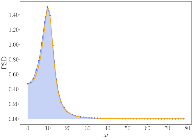
It is interesting to see the behavior of these spectral densities in the case the time scales $r^{-1}$ (the expected time needed for an infected individual to lose immunity) and $\alpha^{-1}$ (the time an infected individual remains contagious) are well separated, i.e. $\alpha\gg r$. To describe the behavior of the spectral density in this regime we keep $r$ and $\rho:=\frac{\alpha}{\lambda}\in(0,1)$ fixed and let $\lambda$, and therefore also $\alpha$, increase to infinity. Note that in this regime, using the notation in (23), $\lambda_{-}\sim\alpha=\rho\lambda<\lambda$ and $\lambda_{+}\sim\frac{4\rho^{2}\lambda^{2}}{r}>\lambda$ for $\lambda$ large. So the condition $\lambda_{-}<\lambda<\lambda_{+}$ is satisfied, and the equilibrium $(m^{\ast},v^{\ast})$ is a stable spiral. Moreover

$$S_{11}(\omega)\sim\frac{2r\left(1-\rho\right)\omega^{2}+r\left(1-\rho\right)\rho^{2}\lambda^{2}}{\left(\omega^{2}-r\left(1-\rho\right)\lambda\right)^{2}+\frac{r^{2}}{\rho^{2}}\omega^{2}}$$

and

$$S_{22}(\omega)\sim\frac{r\left(1-\rho\right)\omega^{2}+r^{3}\frac{1-\rho}{\rho^{2}}+2r^{3}\frac{\left(1-\rho\right)^{3}}{\rho^{2}}-2r^{3}\frac{\left(1-\rho\right)^{2}}{\rho^{2}}}{\left(\omega^{2}-r\left(1-\rho\right)\lambda\right)^{2}+\frac{r^{2}}{\rho^{2}}\omega^{2}}.$$

It is easily seen that, for $\lambda$ large, both spectral densities have a sharp peak around the frequency $\omega^{*}:=\sqrt{r(1-\rho)\lambda}$, as shown in Figure 2: random fluctuations around equilibrium exhibit oscillations with a nearly deterministic period. This analysis motivates the scaling limit performed in next section.

Refer to caption
Figure 2: The spectral density of the process $\xi(t)$ in (30) (in orange) compared to the estimated spectrum of $\xi_{N}$ in (29) (blue points) for the parameters $N=10000$, $r=5$, $\lambda=100$, $\rho=0.7$. To obtain the blue curve, $100$ simulations of system (5) were performed employing an Euler scheme with time-step $0.001$.

5 Rescaling the parameters

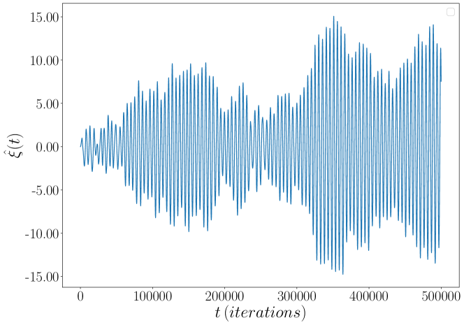
The aim of this section is to obtain the limit behavior of the microscopic dynamics when we let the parameters $\alpha$ and $\lambda$ diverge with $N$. Consistently with what we have seen in Section 4.1, we fix $r>0$, $\rho\in(0,1)$, set $\alpha_{N}=\rho\lambda_{N}$ and let $\lambda_{N}\uparrow+\infty$ as $N\uparrow+\infty$. We have observed that this asymptotics produces a sharp peak in the power spectrum. On the one hand, since the power spectral density reflects the long-time behavior of a process, we do not expect the peak of $S_{11}$ and $S_{22}$ to be due to the damped oscillations which the limit system (16) exhibits when far from equilibrium. On the other hand, for $\lambda\gg r$, by looking at the linearization of system (16) around its stable equilibrium we might expect that (16) behaves as a deterministic harmonic oscillator, the dampening factor acting on very long time scales. In turn, one might think that the sharp peak of the power spectrum essentially captures deterministic oscillations with a negligible dampening. However, numerical simulations of system (29) show oscillations with a nearly deterministic period, but with a random amplitude, hence, different in nature from the ones of a deterministic oscillator. To explain this phenomenon, taking into account that we are interested in the long time behavior, we begin by assuming the initial state $\left(x_{i}(0)\right)_{i=1}^{N}$ to be a system of i.i.d. variables, as in Theorem 4.1, but such that ${\mathbb{P}}(x_{i}(0)>0)=m^{\ast}$, ${\mathbb{E}}[x_{i}(0)]=v^{\ast}$, i.e. the equilibrium values have been attained. For instance, we may assume $x_{i}(0)$ to be distributed according to the $\rho^{\ast}$ defined in (28). The key point now is to find a suitable rescaling of the fluctuations $\left(m_{N}(t)-m^{\ast}\right)$, $\left(v_{N}(t)-v^{\ast}\right)$ to have a nontrivial limit. Note that even propagation of chaos is not obvious anymore: indeed, since some parameters of the model diverge with $N$, the possibility that propagation of chaos deteriorates in short time cannot be ignored. Moreover, if oscillations are detected in the limit, a specific time rescaling is forced by the the previous observation that the asymptotic frequency is of order $\sqrt{\lambda}$.

Theorem 5.1.

Define the rescaled fluctuation processes as follows:

$$\begin{split}&\hat{\xi}^{N}(t)\coloneqq\sqrt{N}\frac{m_{N}\left(\frac{t}{\sqrt{\lambda_{N}}}\right)-m^{\ast}}{\lambda_{N}^{1/4}}\\ &\hat{\eta}^{N}(t)\coloneqq\lambda_{N}^{1/4}\sqrt{N}\left(v_{N}\left(\frac{t}{\sqrt{\lambda_{N}}}\right)-v^{\ast}\right)\end{split}$$ (36)

and assume the initial state $\left(x_{i}(0)\right)_{i=1}^{N}$ to be a system of i.i.d. variables such that ${\mathbb{P}}(x_{i}(0)>0)=m^{\ast}$, ${\mathbb{E}}[x_{i}(0)]=v^{\ast}$. Moreover assume $\alpha_{N}=\rho\lambda_{N}$, and

$$\lim_{N\rightarrow+\infty}\lambda_{N}=+\infty\hskip 56.9055pt\lim_{N\rightarrow+\infty}\frac{\sqrt{\lambda_{N}}}{\log N}=0.$$

Then the process $(\hat{\xi}^{N}(t),\hat{\eta}^{N}(t))^{T}$ converges in distribution, in any interval $[0,T]$, to the random harmonic oscillator

$$\begin{split}d\hat{\xi}(t)&=\rho\hat{\eta}(t)dt\\ d\hat{\eta}(t)&=-\frac{r}{\rho}(1-\rho)\hat{\xi}(t)dt+r(1-\rho)dW(t)\\ \hat{\xi}(0)&=\hat{\eta}(0)=0\end{split}$$ (37)

where $W(t)$ is a standard Brownian motion.

As the simulation in Figure 3 shows, the Brownian noise has little effects on the frequency of the oscillations, which is $\sqrt{r(1-\rho)}$ for the deterministic system, but substantially affects the amplitudes.

Refer to caption
Figure 3: Sample trajectory of $\hat{\xi}(t)$ (system (37)) at stationarity.

6 Proofs

6.1 Proof of Theorem 2.1

It is convenient to set $\sigma_{i}(t):={\bf{1}}_{\{x_{i}(t)>0\}}$, so that (5) can be split into the system

xi​(t)=xi​(0)+∫0tβˆ’Ξ±β€‹xi​(s)​d​s+∫[0,t]Γ—[0,+∞)𝟏[0,(1βˆ’Οƒi​(sβˆ’))​λ​vN​(sβˆ’)]​(u)​Ni↑​(d​s,d​u)βˆ’βˆ«[0,t]Γ—[0,+∞)xi​(sβˆ’)β€‹πŸ[0,Οƒi​(sβˆ’)​r]​(u)​Ni↓​(d​s,d​u)Οƒi​(t)=Οƒi​(0)+∫[0,t]Γ—[0,+∞)𝟏[0,(1βˆ’Οƒi​(sβˆ’))​λ​vN​(sβˆ’)]​(u)​Ni↑​(d​s,d​u)βˆ’βˆ«[0,t]Γ—[0,+∞)𝟏[0,Οƒi​(sβˆ’)​r]​(u)​Ni↓​(d​s,d​u).subscriptπ‘₯𝑖𝑑subscriptπ‘₯𝑖0superscriptsubscript0𝑑𝛼subscriptπ‘₯𝑖𝑠𝑑𝑠subscript0𝑑0subscript101subscriptπœŽπ‘–superscriptπ‘ πœ†subscript𝑣𝑁superscript𝑠𝑒subscriptsuperscript𝑁↑𝑖𝑑𝑠𝑑𝑒subscript0𝑑0subscriptπ‘₯𝑖superscript𝑠subscript10subscriptπœŽπ‘–superscriptπ‘ π‘Ÿπ‘’subscriptsuperscript𝑁↓𝑖𝑑𝑠𝑑𝑒subscriptπœŽπ‘–π‘‘subscriptπœŽπ‘–0subscript0𝑑0subscript101subscriptπœŽπ‘–superscriptπ‘ πœ†subscript𝑣𝑁superscript𝑠𝑒subscriptsuperscript𝑁↑𝑖𝑑𝑠𝑑𝑒subscript0𝑑0subscript10subscriptπœŽπ‘–superscriptπ‘ π‘Ÿπ‘’subscriptsuperscript𝑁↓𝑖𝑑𝑠𝑑𝑒\begin{split}x_{i}(t)&=x_{i}(0)+\int_{0}^{t}-\alpha x_{i}(s)ds+\int_{[0,t]\times[0,+\infty)}\boldsymbol{1}_{[0,(1-\sigma_{i}(s^{-}))\lambda v_{N}(s^{-})]}(u)N^{\uparrow}_{i}(ds,du)\\ &-\int_{[0,t]\times[0,+\infty)}x_{i}(s^{-})\boldsymbol{1}_{[0,\sigma_{i}(s^{-})r]}(u)N^{\downarrow}_{i}(ds,du)\\ \sigma_{i}(t)&=\sigma_{i}(0)+\int_{[0,t]\times[0,+\infty)}\boldsymbol{1}_{[0,(1-\sigma_{i}(s^{-}))\lambda v_{N}(s^{-})]}(u)N^{\uparrow}_{i}(ds,du)\\ &-\int_{[0,t]\times[0,+\infty)}\boldsymbol{1}_{[0,\sigma_{i}(s^{-})r]}(u)N^{\downarrow}_{i}(ds,du).\end{split} (38)

A similar splitting applies to the limiting equation (6) if we define $\bar{\sigma}_{i}(t):={\bf{1}}_{\{\bar{x}_{i}(t)>0\}}$:

xΒ―i​(t)=xi​(0)+∫0tβˆ’Ξ±β€‹xΒ―i​(s)​d​s+∫[0,t]Γ—[0,+∞)𝟏[0,(1βˆ’ΟƒΒ―i​(sβˆ’))​λ​v​(sβˆ’)]​(u)​Ni↑​(d​s,d​u)βˆ’βˆ«[0,t]Γ—[0,+∞)xΒ―i​(sβˆ’)β€‹πŸ[0,σ¯i​(sβˆ’)​r]​(u)​Ni↓​(d​s,d​u)σ¯i​(t)=Οƒi​(0)+∫[0,t]Γ—[0,+∞)𝟏[0,(1βˆ’ΟƒΒ―i​(sβˆ’))​λ​v​(sβˆ’)]​(u)​Ni↑​(d​s,d​u)βˆ’βˆ«[0,t]Γ—[0,+∞)𝟏[0,σ¯i​(sβˆ’)​r]​(u)​Ni↓​(d​s,d​u)subscriptΒ―π‘₯𝑖𝑑subscriptπ‘₯𝑖0superscriptsubscript0𝑑𝛼subscriptΒ―π‘₯𝑖𝑠𝑑𝑠subscript0𝑑0subscript101subscriptΒ―πœŽπ‘–superscriptπ‘ πœ†π‘£superscript𝑠𝑒superscriptsubscript𝑁𝑖↑𝑑𝑠𝑑𝑒subscript0𝑑0subscriptΒ―π‘₯𝑖superscript𝑠subscript10subscriptΒ―πœŽπ‘–superscriptπ‘ π‘Ÿπ‘’superscriptsubscript𝑁𝑖↓𝑑𝑠𝑑𝑒subscriptΒ―πœŽπ‘–π‘‘subscriptπœŽπ‘–0subscript0𝑑0subscript101subscriptΒ―πœŽπ‘–superscriptπ‘ πœ†π‘£superscript𝑠𝑒subscriptsuperscript𝑁↑𝑖𝑑𝑠𝑑𝑒subscript0𝑑0subscript10subscriptΒ―πœŽπ‘–superscriptπ‘ π‘Ÿπ‘’subscriptsuperscript𝑁↓𝑖𝑑𝑠𝑑𝑒\begin{split}\bar{x}_{i}(t)&=x_{i}(0)+\int_{0}^{t}-\alpha\bar{x}_{i}(s)ds+\int_{[0,t]\times[0,+\infty)}\boldsymbol{1}_{[0,(1-\bar{\sigma}_{i}(s^{-}))\lambda v(s^{-})]}(u)N_{i}^{\uparrow}(ds,du)\\ &-\int_{[0,t]\times[0,+\infty)}\bar{x}_{i}(s^{-})\boldsymbol{1}_{[0,\bar{\sigma}_{i}(s^{-})r]}(u)N_{i}^{\downarrow}(ds,du)\\ \bar{\sigma}_{i}(t)&=\sigma_{i}(0)+\int_{[0,t]\times[0,+\infty)}\boldsymbol{1}_{[0,(1-\bar{\sigma}_{i}(s^{-}))\lambda v(s^{-})]}(u)N^{\uparrow}_{i}(ds,du)\\ &-\int_{[0,t]\times[0,+\infty)}\boldsymbol{1}_{[0,\bar{\sigma}_{i}(s^{-})r]}(u)N^{\downarrow}_{i}(ds,du)\end{split} (39)

It follows that

|xi​(t)βˆ’xΒ―i​(t)|β‰€Ξ±β€‹βˆ«0t|xi​(s)βˆ’xΒ―i​(s)|​𝑑s+∫[0,t]Γ—[0,+∞)|𝟏[0,(1βˆ’Οƒi​(sβˆ’))​λ​vN​(sβˆ’)]​(u)βˆ’πŸ[0,(1βˆ’ΟƒΒ―i​(sβˆ’))​λ​v​(sβˆ’)]​(u)|Ni↑​(d​s,d​u)+∫[0,t]Γ—[0,+∞)|xi​(sβˆ’)β€‹πŸ[0,Οƒi​(sβˆ’)​r]​(u)βˆ’xΒ―i​(sβˆ’)β€‹πŸ[0,σ¯i​(sβˆ’)​r]​(u)|​Ni↓​(d​s,d​u)subscriptπ‘₯𝑖𝑑subscriptΒ―π‘₯𝑖𝑑𝛼superscriptsubscript0𝑑subscriptπ‘₯𝑖𝑠subscriptΒ―π‘₯𝑖𝑠differential-d𝑠subscript0𝑑0subscript101subscriptπœŽπ‘–superscriptπ‘ πœ†subscript𝑣𝑁superscript𝑠𝑒subscript101subscriptΒ―πœŽπ‘–superscriptπ‘ πœ†π‘£superscript𝑠𝑒superscriptsubscript𝑁𝑖↑𝑑𝑠𝑑𝑒subscript0𝑑0subscriptπ‘₯𝑖superscript𝑠subscript10subscriptπœŽπ‘–superscriptπ‘ π‘Ÿπ‘’subscriptΒ―π‘₯𝑖superscript𝑠subscript10subscriptΒ―πœŽπ‘–superscriptπ‘ π‘Ÿπ‘’superscriptsubscript𝑁𝑖↓𝑑𝑠𝑑𝑒\begin{split}|x_{i}(t)-\bar{x}_{i}(t)|&\leq\alpha\int_{0}^{t}|x_{i}(s)-\bar{x}_{i}(s)|ds+\int_{[0,t]\times[0,+\infty)}\left|\boldsymbol{1}_{[0,(1-\sigma_{i}(s^{-}))\lambda v_{N}(s^{-})]}(u)\right.\\ &\left.-\boldsymbol{1}_{[0,(1-\bar{\sigma}_{i}(s^{-}))\lambda v(s^{-})]}(u)\right|N_{i}^{\uparrow}(ds,du)\\ &+\int_{[0,t]\times[0,+\infty)}\left|x_{i}(s^{-})\boldsymbol{1}_{[0,\sigma_{i}(s^{-})r]}(u)-\bar{x}_{i}(s^{-})\boldsymbol{1}_{[0,\bar{\sigma}_{i}(s^{-})r]}(u)\right|N_{i}^{\downarrow}(ds,du)\end{split} (40)

and similarly

|Οƒi​(t)βˆ’ΟƒΒ―i​(t)|β‰€βˆ«[0,t]Γ—[0,+∞)|𝟏[0,(1βˆ’Οƒi​(sβˆ’))​λ​vN​(sβˆ’)]​(u)βˆ’πŸ[0,(1βˆ’ΟƒΒ―i​(sβˆ’))​λ​v​(sβˆ’)]​(u)|​Ni↑​(d​s,d​u)+∫[0,t]Γ—[0,+∞)|𝟏[0,Οƒi​(sβˆ’)​r]​(u)βˆ’πŸ[0,σ¯i​(sβˆ’)​r]​(u)|​Ni↓​(d​s,d​u).subscriptπœŽπ‘–π‘‘subscriptΒ―πœŽπ‘–π‘‘subscript0𝑑0subscript101subscriptπœŽπ‘–superscriptπ‘ πœ†subscript𝑣𝑁superscript𝑠𝑒subscript101subscriptΒ―πœŽπ‘–superscriptπ‘ πœ†π‘£superscript𝑠𝑒subscriptsuperscript𝑁↑𝑖𝑑𝑠𝑑𝑒subscript0𝑑0subscript10subscriptπœŽπ‘–superscriptπ‘ π‘Ÿπ‘’subscript10subscriptΒ―πœŽπ‘–superscriptπ‘ π‘Ÿπ‘’subscriptsuperscript𝑁↓𝑖𝑑𝑠𝑑𝑒\begin{split}|\sigma_{i}(t)-\bar{\sigma}_{i}(t)|&\leq\int_{[0,t]\times[0,+\infty)}\left|\boldsymbol{1}_{[0,(1-\sigma_{i}(s^{-}))\lambda v_{N}(s^{-})]}(u)-\boldsymbol{1}_{[0,(1-\bar{\sigma}_{i}(s^{-}))\lambda v(s^{-})]}(u)\right|N^{\uparrow}_{i}(ds,du)\\ &+\int_{[0,t]\times[0,+\infty)}\left|\boldsymbol{1}_{[0,\sigma_{i}(s^{-})r]}(u)-\boldsymbol{1}_{[0,\bar{\sigma}_{i}(s^{-})r]}(u)\right|N^{\downarrow}_{i}(ds,du).\end{split} (41)

Note that both in (40) and (41), by increasingness of the integrals in the r.h.s, the l.h.s. can be replaced by $\sup_{s\leq t}|x_{i}(s)-\bar{x}_{i}(s)|$ and sups≀t|Οƒi​(s)βˆ’ΟƒΒ―i​(s)|subscriptsupremum𝑠𝑑subscriptπœŽπ‘–π‘ subscriptΒ―πœŽπ‘–π‘ \sup_{s\leq t}|\sigma_{i}(s)-\bar{\sigma}_{i}(s)| respectively. Taking expectation and letting

φ​(t)=𝔼​[sup0≀s≀t(|xi​(s)βˆ’xΒ―i​(s)|+|Οƒi​(s)βˆ’ΟƒΒ―i​(s)|)],πœ‘π‘‘π”Όdelimited-[]subscriptsupremum0𝑠𝑑subscriptπ‘₯𝑖𝑠subscriptΒ―π‘₯𝑖𝑠subscriptπœŽπ‘–π‘ subscriptΒ―πœŽπ‘–π‘ \varphi(t)={\mathbb{E}}\left[\sup_{0\leq s\leq t}\left(|x_{i}(s)-\bar{x}_{i}(s)|+|\sigma_{i}(s)-\bar{\sigma}_{i}(s)|\right)\right],\

we obtain

φ​(t)β‰€Ξ±β€‹βˆ«0tφ​(s)​𝑑s+𝔼​[∫[0,t]Γ—[0,+∞)|𝟏[0,(1βˆ’Οƒi​(sβˆ’))​λ​vN​(sβˆ’)]​(u)βˆ’πŸ[0,(1βˆ’ΟƒΒ―i​(sβˆ’))​λ​v​(sβˆ’)]​(u)|​Ni↑​(d​s,d​u)]+𝔼​[∫[0,t]Γ—[0,+∞)|xi​(sβˆ’)β€‹πŸ[0,Οƒi​(sβˆ’)​r]​(u)βˆ’xΒ―i​(sβˆ’)β€‹πŸ[0,σ¯i​(sβˆ’)​r]​(u)|​Ni↓​(d​s,d​u)]+𝔼​[∫[0,t]Γ—[0,+∞)|𝟏[0,(1βˆ’Οƒi​(sβˆ’))​λ​vN​(sβˆ’)]​(u)βˆ’πŸ[0,(1βˆ’ΟƒΒ―i​(sβˆ’))​λ​v​(sβˆ’)]​(u)|​Ni↑​(d​s,d​u)]+𝔼​[∫[0,t]Γ—[0,+∞)|𝟏[0,Οƒi​(sβˆ’)​r]​(u)βˆ’πŸ[0,σ¯i​(sβˆ’)​r]​(u)|​Ni↓​(d​s,d​u)]πœ‘π‘‘π›Όsuperscriptsubscript0π‘‘πœ‘π‘ differential-d𝑠𝔼delimited-[]subscript0𝑑0subscript101subscriptπœŽπ‘–superscriptπ‘ πœ†subscript𝑣𝑁superscript𝑠𝑒subscript101subscriptΒ―πœŽπ‘–superscriptπ‘ πœ†π‘£superscript𝑠𝑒superscriptsubscript𝑁𝑖↑𝑑𝑠𝑑𝑒𝔼delimited-[]subscript0𝑑0subscriptπ‘₯𝑖superscript𝑠subscript10subscriptπœŽπ‘–superscriptπ‘ π‘Ÿπ‘’subscriptΒ―π‘₯𝑖superscript𝑠subscript10subscriptΒ―πœŽπ‘–superscriptπ‘ π‘Ÿπ‘’superscriptsubscript𝑁𝑖↓𝑑𝑠𝑑𝑒𝔼delimited-[]subscript0𝑑0subscript101subscriptπœŽπ‘–superscriptπ‘ πœ†subscript𝑣𝑁superscript𝑠𝑒subscript101subscriptΒ―πœŽπ‘–superscriptπ‘ πœ†π‘£superscript𝑠𝑒subscriptsuperscript𝑁↑𝑖𝑑𝑠𝑑𝑒𝔼delimited-[]subscript0𝑑0subscript10subscriptπœŽπ‘–superscriptπ‘ π‘Ÿπ‘’subscript10subscriptΒ―πœŽπ‘–superscriptπ‘ π‘Ÿπ‘’subscriptsuperscript𝑁↓𝑖𝑑𝑠𝑑𝑒\begin{split}\varphi(t)&\leq\alpha\int_{0}^{t}\varphi(s)ds\\ &+{\mathbb{E}}\left[\int_{[0,t]\times[0,+\infty)}\left|\boldsymbol{1}_{[0,(1-\sigma_{i}(s^{-}))\lambda v_{N}(s^{-})]}(u)-\boldsymbol{1}_{[0,(1-\bar{\sigma}_{i}(s^{-}))\lambda v(s^{-})]}(u)\right|N_{i}^{\uparrow}(ds,du)\right]\\ &+{\mathbb{E}}\left[\int_{[0,t]\times[0,+\infty)}\left|x_{i}(s^{-})\boldsymbol{1}_{[0,\sigma_{i}(s^{-})r]}(u)-\bar{x}_{i}(s^{-})\boldsymbol{1}_{[0,\bar{\sigma}_{i}(s^{-})r]}(u)\right|N_{i}^{\downarrow}(ds,du)\right]\\ &+{\mathbb{E}}\left[\int_{[0,t]\times[0,+\infty)}\left|\boldsymbol{1}_{[0,(1-\sigma_{i}(s^{-}))\lambda v_{N}(s^{-})]}(u)-\boldsymbol{1}_{[0,(1-\bar{\sigma}_{i}(s^{-}))\lambda v(s^{-})]}(u)\right|N^{\uparrow}_{i}(ds,du)\right]\\ &+{\mathbb{E}}\left[\int_{[0,t]\times[0,+\infty)}\left|\boldsymbol{1}_{[0,\sigma_{i}(s^{-})r]}(u)-\boldsymbol{1}_{[0,\bar{\sigma}_{i}(s^{-})r]}(u)\right|N^{\downarrow}_{i}(ds,du)\right]\end{split} (42)

We now use the following facts: if $f(s,u)$ is bounded, positive and predictable then

$${\mathbb{E}}\left[\int_{[0,t]\times[0,+\infty)}f(s,u)N_{i}^{\uparrow}(ds,du)\right]={\mathbb{E}}\left[\int_{[0,t]\times[0,+\infty)}f(s,u)duds\right]$$ (43)

and, for $a,a^{\prime},b,b^{\prime}\geq 0$

$$\int_{0}^{+\infty}\left|a\boldsymbol{1}_{[0,b]}(u)-a^{\prime}\boldsymbol{1}_{[0,b^{\prime}]}(u)\right|du\leq a|b-b^{\prime}|+b^{\prime}|a-a^{\prime}|.$$

This yields

𝔼[∫[0,t]Γ—[0,+∞)|𝟏[0,(1βˆ’Οƒi​(sβˆ’))​λ​vN​(sβˆ’)]​(u)βˆ’πŸ[0,(1βˆ’ΟƒΒ―i​(sβˆ’))​λ​v​(sβˆ’)]​(u)|​Ni↑​(d​s,d​u)]=λ​𝔼​[∫0t|(1βˆ’Οƒi​(s))​vN​(s)βˆ’(1βˆ’ΟƒΒ―i​(s))​v​(s)|​𝑑s]≀λ​𝔼​[∫0t|Οƒi​(s)βˆ’ΟƒΒ―i​(s)|​𝑑s]+λ​𝔼​[∫0t|vN​(s)βˆ’v​(s)|​𝑑s]β‰€Ξ»β€‹βˆ«0tφ​(s)​𝑑s+λ​𝔼​[∫0t|vN​(s)βˆ’v​(s)|​𝑑s]𝔼delimited-[]subscript0𝑑0subscript101subscriptπœŽπ‘–superscriptπ‘ πœ†subscript𝑣𝑁superscript𝑠𝑒subscript101subscriptΒ―πœŽπ‘–superscriptπ‘ πœ†π‘£superscript𝑠𝑒superscriptsubscriptπ‘π‘–β†‘π‘‘π‘ π‘‘π‘’πœ†π”Όdelimited-[]superscriptsubscript0𝑑1subscriptπœŽπ‘–π‘ subscript𝑣𝑁𝑠1subscriptΒ―πœŽπ‘–π‘ π‘£π‘ differential-dπ‘ πœ†π”Όdelimited-[]superscriptsubscript0𝑑subscriptπœŽπ‘–π‘ subscriptΒ―πœŽπ‘–π‘ differential-dπ‘ πœ†π”Όdelimited-[]superscriptsubscript0𝑑subscript𝑣𝑁𝑠𝑣𝑠differential-dπ‘ πœ†superscriptsubscript0π‘‘πœ‘π‘ differential-dπ‘ πœ†π”Όdelimited-[]superscriptsubscript0𝑑subscript𝑣𝑁𝑠𝑣𝑠differential-d𝑠\begin{split}{\mathbb{E}}&\left[\int_{[0,t]\times[0,+\infty)}\left|\boldsymbol{1}_{[0,(1-\sigma_{i}(s^{-}))\lambda v_{N}(s^{-})]}(u)-\boldsymbol{1}_{[0,(1-\bar{\sigma}_{i}(s^{-}))\lambda v(s^{-})]}(u)\right|N_{i}^{\uparrow}(ds,du)\right]\\ &=\lambda{\mathbb{E}}\left[\int_{0}^{t}\left|(1-\sigma_{i}(s))v_{N}(s)-(1-\bar{\sigma}_{i}(s))v(s)\right|ds\right]\\ &\leq\lambda{\mathbb{E}}\left[\int_{0}^{t}|\sigma_{i}(s)-\bar{\sigma}_{i}(s)|ds\right]+\lambda{\mathbb{E}}\left[\int_{0}^{t}|v_{N}(s)-v(s)|ds\right]\\ &\leq\lambda\int_{0}^{t}\varphi(s)ds+\lambda{\mathbb{E}}\left[\int_{0}^{t}|v_{N}(s)-v(s)|ds\right]\end{split} (44)

Similarly

𝔼[∫[0,t]Γ—[0,+∞)|xi​(sβˆ’)β€‹πŸ[0,Οƒi​(sβˆ’)​r]​(u)βˆ’xΒ―i​(sβˆ’)β€‹πŸ[0,σ¯i​(sβˆ’)​r]​(u)|​Ni↓​(d​s,d​u)]≀r​𝔼​[∫0t|xi​(s)βˆ’xΒ―i​(s)|​𝑑s]+r​𝔼​[∫0t|Οƒi​(s)βˆ’ΟƒΒ―i​(s)|​𝑑s]≀rβ€‹βˆ«0tφ​(s)​𝑑s,𝔼delimited-[]subscript0𝑑0subscriptπ‘₯𝑖superscript𝑠subscript10subscriptπœŽπ‘–superscriptπ‘ π‘Ÿπ‘’subscriptΒ―π‘₯𝑖superscript𝑠subscript10subscriptΒ―πœŽπ‘–superscriptπ‘ π‘Ÿπ‘’superscriptsubscriptπ‘π‘–β†“π‘‘π‘ π‘‘π‘’π‘Ÿπ”Όdelimited-[]superscriptsubscript0𝑑subscriptπ‘₯𝑖𝑠subscriptΒ―π‘₯𝑖𝑠differential-dπ‘ π‘Ÿπ”Όdelimited-[]superscriptsubscript0𝑑subscriptπœŽπ‘–π‘ subscriptΒ―πœŽπ‘–π‘ differential-dπ‘ π‘Ÿsuperscriptsubscript0π‘‘πœ‘π‘ differential-d𝑠\begin{split}{\mathbb{E}}&\left[\int_{[0,t]\times[0,+\infty)}\left|x_{i}(s^{-})\boldsymbol{1}_{[0,\sigma_{i}(s^{-})r]}(u)-\bar{x}_{i}(s^{-})\boldsymbol{1}_{[0,\bar{\sigma}_{i}(s^{-})r]}(u)\right|N_{i}^{\downarrow}(ds,du)\right]\\ &\leq r{\mathbb{E}}\left[\int_{0}^{t}|x_{i}(s)-\bar{x}_{i}(s)|ds\right]+r{\mathbb{E}}\left[\int_{0}^{t}|\sigma_{i}(s)-\bar{\sigma}_{i}(s)|ds\right]\\ &\leq r\int_{0}^{t}\varphi(s)ds,\end{split} (45)

Estimating in the same way the other two terms in the r.h.s. of (42), from (42), (44) and (45) we obtain

φ​(t)≀(Ξ±+2​λ+2​r)β€‹βˆ«0tφ​(s)​𝑑s+λ​𝔼​[∫0t|vN​(s)βˆ’v​(s)|​𝑑s].πœ‘π‘‘π›Ό2πœ†2π‘Ÿsuperscriptsubscript0π‘‘πœ‘π‘ differential-dπ‘ πœ†π”Όdelimited-[]superscriptsubscript0𝑑subscript𝑣𝑁𝑠𝑣𝑠differential-d𝑠\varphi(t)\leq(\alpha+2\lambda+2r)\int_{0}^{t}\varphi(s)ds+\lambda{\mathbb{E}}\left[\int_{0}^{t}|v_{N}(s)-v(s)|ds\right]. (46)

Noticing that, letting $\bar{v}_{N}(s)\coloneqq\frac{1}{N}\sum_{i=1}^{N}\bar{x}_{i}(s)$,

$$\begin{split}{\mathbb{E}}\left[|v_{N}(s)-v(s)|\right]&\leq{\mathbb{E}}\left[|v_{N}(s)-\bar{v}_{N}(s)|\right]+{\mathbb{E}}\left[|\bar{v}_{N}(s)-v(s)|\right]\leq\phi(s)+\left(\mbox{Var}(\bar{v}_{N}(s))\right)^{1/2}\\ &\leq\phi(s)+\frac{1}{\sqrt{N}},\end{split}$$

we finally obtain from (46)

φ​(t)≀(Ξ±+3​λ+2​r)β€‹βˆ«0tφ​(s)​𝑑s+λ​TN.πœ‘π‘‘π›Ό3πœ†2π‘Ÿsuperscriptsubscript0π‘‘πœ‘π‘ differential-dπ‘ πœ†π‘‡π‘\varphi(t)\leq(\alpha+3\lambda+2r)\int_{0}^{t}\varphi(s)ds+\frac{\lambda T}{\sqrt{N}}.

A direct application of Gromwall Lemma provides

$$\varphi(T)\leq\frac{\lambda T}{\sqrt{N}}e^{(\alpha+3\lambda+2r)T},$$

and the proof is complete.

6.2 Proof of Corollary 2.2

By adding and subtracting $\bar{m}_{N}(t)\coloneqq\frac{1}{N}\sum_{i=1}^{N}\bar{\sigma}_{i}(t)$,

$$\begin{split}{\mathbb{E}}\left[\sup_{t\in[0,T]}\left|m_{N}(t)-{\mathbb{P}}[\bar{x}(t)>0]\right|\right]&\leq{\mathbb{E}}\left[\sup_{t\in[0,T]}\left|m_{N}(t)-\bar{m}_{N}(t)\right|\right]+{\mathbb{E}}\left[\sup_{t\in[0,T]}\left|\bar{m}_{N}(t)-m(t)\right|\right]\\ &\leq\frac{1}{N}\sum_{i=1}^{N}{\mathbb{E}}\left[\sup_{t\in[0,T]}\left|\sigma_{i}(t)-\bar{\sigma}_{i}(t)\right|\right]+{\mathbb{E}}\left[\sup_{t\in[0,T]}\left|\bar{m}_{N}(t)-m(t)\right|\right]\end{split}$$ (47)

The first term in the r.h.s. of (47), by Theorem 2.1, is bounded by $\frac{A_{T}}{\sqrt{N}}$. So we show that a similar bound holds for the second term in the r.h.s. of (47). Averaging over $i$ in (39) we get

mΒ―N​(t)=mΒ―N​(0)+∫0t(λ​v​(s)​(1βˆ’mΒ―N​(s))βˆ’r​mΒ―N​(s))​𝑑s+1N​MN​(t)subscriptΒ―π‘šπ‘π‘‘subscriptΒ―π‘šπ‘0superscriptsubscript0π‘‘πœ†π‘£π‘ 1subscriptΒ―π‘šπ‘π‘ π‘ŸsubscriptΒ―π‘šπ‘π‘ differential-d𝑠1𝑁subscript𝑀𝑁𝑑\bar{m}_{N}(t)=\bar{m}_{N}(0)+\int_{0}^{t}\left(\lambda v(s)(1-\bar{m}_{N}(s))-r\bar{m}_{N}(s)\right)ds+\frac{1}{N}M_{N}(t) (48)

with

MN​(t)=βˆ‘i=1N[∫[0,t]Γ—[0,+∞)𝟏[0,(1βˆ’ΟƒΒ―i​(sβˆ’))​λ​v​(sβˆ’)]​(u)​N~i↑​(d​s,d​u)βˆ’βˆ«[0,t]Γ—[0,+∞)𝟏[0,σ¯i​(sβˆ’)​r]​(u)​N~i↓​(d​s,d​u)],subscript𝑀𝑁𝑑superscriptsubscript𝑖1𝑁delimited-[]subscript0𝑑0subscript101subscriptΒ―πœŽπ‘–superscriptπ‘ πœ†π‘£superscript𝑠𝑒subscriptsuperscript~𝑁↑𝑖𝑑𝑠𝑑𝑒subscript0𝑑0subscript10subscriptΒ―πœŽπ‘–superscriptπ‘ π‘Ÿπ‘’subscriptsuperscript~𝑁↓𝑖𝑑𝑠𝑑𝑒M_{N}(t)=\sum_{i=1}^{N}\left[\int_{[0,t]\times[0,+\infty)}\boldsymbol{1}_{[0,(1-\bar{\sigma}_{i}(s^{-}))\lambda v(s^{-})]}(u)\tilde{N}^{\uparrow}_{i}(ds,du)-\int_{[0,t]\times[0,+\infty)}\boldsymbol{1}_{[0,\bar{\sigma}_{i}(s^{-})r]}(u)\tilde{N}^{\downarrow}_{i}(ds,du)\right], (49)

where we have introduced the compensated Poisson random measures defined by

$$\begin{split}\tilde{N}^{\uparrow}_{i}(ds,du)&:=N^{\uparrow}_{i}(ds,du)-dsdu\\ \tilde{N}^{\downarrow}_{i}(ds,du)&:=N^{\downarrow}_{i}(ds,du)-dsdu.\end{split}$$ (50)

We recall that for a predictable, positive and bounded $f(s,u)$ such that

$${\mathbb{E}}\left[\int_{[0,T]\times[0,+\infty)}f^{2}(s,u)dsdu\right]<+\infty,$$

the integrals

$$I_{i}(t):=\int_{[0,t]\times[0,+\infty)}f(s,u)\tilde{N}^{\uparrow}_{i}(ds,du)$$

define orthogonal martingales with quadratic variation $\int_{[0,t]\times[0,+\infty)}f^{2}(s,u)dsdu$. It follows that $M_{N}(t)$ is a martingale having quadratic variation equal to βˆ‘i=1N∫0t[λ​v​(s)​(1βˆ’ΟƒΒ―i​(s))+r​σ¯i​(s)]​𝑑ssuperscriptsubscript𝑖1𝑁superscriptsubscript0𝑑delimited-[]πœ†π‘£π‘ 1subscriptΒ―πœŽπ‘–π‘ π‘ŸsubscriptΒ―πœŽπ‘–π‘ differential-d𝑠\sum_{i=1}^{N}\int_{0}^{t}[\lambda v(s)(1-\bar{\sigma}_{i}(s))+r\bar{\sigma}_{i}(s)]ds. From (16) we also obtain

m​(t)=m​(0)+∫0t(λ​v​(s)​(1βˆ’m​(s))βˆ’r​m​(s))​𝑑s.π‘šπ‘‘π‘š0superscriptsubscript0π‘‘πœ†π‘£π‘ 1π‘šπ‘ π‘Ÿπ‘šπ‘ differential-d𝑠m(t)=m(0)+\int_{0}^{t}\left(\lambda v(s)(1-m(s))-rm(s)\right)ds. (51)

From (48) and (51) we get

|mΒ―N​(t)βˆ’m​(t)|≀|mΒ―N​(0)βˆ’m​(0)|+∫0t(λ​v​(s)+r)​|mΒ―N​(s)βˆ’m​(s)|​𝑑s+1N​|MN​(t)|≀|mΒ―N​(0)βˆ’m​(0)|+∫0t(Ξ»+r)​|mΒ―N​(s)βˆ’m​(s)|​𝑑s+1N​|MN​(t)|.subscriptΒ―π‘šπ‘π‘‘π‘šπ‘‘subscriptΒ―π‘šπ‘0π‘š0superscriptsubscript0π‘‘πœ†π‘£π‘ π‘ŸsubscriptΒ―π‘šπ‘π‘ π‘šπ‘ differential-d𝑠1𝑁subscript𝑀𝑁𝑑subscriptΒ―π‘šπ‘0π‘š0superscriptsubscript0π‘‘πœ†π‘ŸsubscriptΒ―π‘šπ‘π‘ π‘šπ‘ differential-d𝑠1𝑁subscript𝑀𝑁𝑑\begin{split}|\bar{m}_{N}(t)-m(t)|&\leq|\bar{m}_{N}(0)-m(0)|+\int_{0}^{t}(\lambda v(s)+r)|\bar{m}_{N}(s)-m(s)|ds+\frac{1}{N}|M_{N}(t)|\\ &\leq|\bar{m}_{N}(0)-m(0)|+\int_{0}^{t}(\lambda+r)|\bar{m}_{N}(s)-m(s)|ds+\frac{1}{N}|M_{N}(t)|.\end{split} (52)

Observe that, by independence of the components,

$${\mathbb{E}}\left[|\bar{m}_{N}(0)-m(0)|\right]\leq\left(\mbox{Var}(\bar{m}_{N}(0))\right)^{1/2}\leq\frac{1}{\sqrt{N}}.$$

Letting

φ​(t):=𝔼​[sups∈[0,t]|mΒ―N​(s)βˆ’m​(s)|],assignπœ‘π‘‘π”Όdelimited-[]subscriptsupremum𝑠0𝑑subscriptΒ―π‘šπ‘π‘ π‘šπ‘ \varphi(t):={\mathbb{E}}\left[\sup_{s\in[0,t]}|\bar{m}_{N}(s)-m(s)|\right],

using the Burkholder-Davis-Gundy inequality in $L^{1}$ and Jensen’s inequality we obtain from (52)

φ​(t)≀1N+(Ξ»+r)β€‹βˆ«0tφ​(s)​𝑑s+1N​𝔼​[supt∈[0,T]|MN​(t)|]≀1N+(Ξ»+r)β€‹βˆ«0tφ​(s)​𝑑s+K1N​𝔼​[(βˆ‘i=1N∫0t[λ​v​(s)​(1βˆ’ΟƒΒ―i​(s))+r​σ¯i​(s)]​𝑑s)1/2]≀1N+(Ξ»+r)β€‹βˆ«0tφ​(s)​𝑑s+K1N​(∫0T[λ​v​(s)​(1βˆ’mΒ―N​(s))+r​mΒ―N​(s)]​𝑑s)1/2≀1N+(Ξ»+r)β€‹βˆ«0tφ​(s)​𝑑s+K1​T​(Ξ»+r)N.πœ‘π‘‘1π‘πœ†π‘Ÿsuperscriptsubscript0π‘‘πœ‘π‘ differential-d𝑠1𝑁𝔼delimited-[]subscriptsupremum𝑑0𝑇subscript𝑀𝑁𝑑1π‘πœ†π‘Ÿsuperscriptsubscript0π‘‘πœ‘π‘ differential-d𝑠subscript𝐾1𝑁𝔼delimited-[]superscriptsuperscriptsubscript𝑖1𝑁superscriptsubscript0𝑑delimited-[]πœ†π‘£π‘ 1subscriptΒ―πœŽπ‘–π‘ π‘ŸsubscriptΒ―πœŽπ‘–π‘ differential-d𝑠121π‘πœ†π‘Ÿsuperscriptsubscript0π‘‘πœ‘π‘ differential-d𝑠subscript𝐾1𝑁superscriptsuperscriptsubscript0𝑇delimited-[]πœ†π‘£π‘ 1subscriptΒ―π‘šπ‘π‘ π‘ŸsubscriptΒ―π‘šπ‘π‘ differential-d𝑠121π‘πœ†π‘Ÿsuperscriptsubscript0π‘‘πœ‘π‘ differential-d𝑠subscript𝐾1π‘‡πœ†π‘Ÿπ‘\begin{split}\varphi(t)&\leq\frac{1}{\sqrt{N}}+(\lambda+r)\int_{0}^{t}\varphi(s)ds+\frac{1}{N}{\mathbb{E}}\left[\sup_{t\in[0,T]}|M_{N}(t)|\right]\\ &\leq\frac{1}{\sqrt{N}}+(\lambda+r)\int_{0}^{t}\varphi(s)ds+\frac{K_{1}}{N}{\mathbb{E}}\left[\left(\sum_{i=1}^{N}\int_{0}^{t}[\lambda v(s)(1-\bar{\sigma}_{i}(s))+r\bar{\sigma}_{i}(s)]ds\right)^{1/2}\right]\\ &\leq\frac{1}{\sqrt{N}}+(\lambda+r)\int_{0}^{t}\varphi(s)ds+\frac{K_{1}}{\sqrt{N}}\left(\int_{0}^{T}[\lambda v(s)(1-\bar{m}_{N}(s))+r\bar{m}_{N}(s)]ds\right)^{1/2}\\ &\leq\frac{1}{\sqrt{N}}+(\lambda+r)\int_{0}^{t}\varphi(s)ds+\frac{K_{1}\sqrt{T(\lambda+r)}}{\sqrt{N}}.\end{split}

giving

$$\varphi(T)\leq\frac{1+K_{1}\sqrt{T(\lambda+r)}}{\sqrt{N}}e^{(\lambda+r)T}.$$ (53)

By this estimate, (47) and Theorem 2.1, we obtain the desired estimate for ${\mathbb{E}}\left[\sup_{t\in[0,T]}\left|m_{N}(t)-{\mathbb{P}}\left[\bar{x}(t)>0\right]\right|\right]$. The estimate for ${\mathbb{E}}\left[\sup_{t\in[0,T]}\left|v_{N}(t)-{\mathbb{E}}\left[\bar{x}(t)\right]\right|\right]$ follows exactly the same steps, and it is omitted. So we are left to show (12). We begin by observing that, letting $\bar{v}_{N,2}(t)\coloneqq\frac{1}{N}\sum_{i=1}^{N}\bar{x}^{2}_{i}(t)$,

$$\begin{split}{\mathbb{E}}\left[\sup_{t\in[0,T]}\left|v_{N,2}(t)-{\mathbb{E}}\left[\bar{x}^{2}(t)\right]\right|\right]&\leq\frac{1}{N}\sum_{i=1}^{N}{\mathbb{E}}\left[\sup_{t\in[0,T]}|x_{i}^{2}(t)-\bar{x}_{i}^{2}(t)|\right]+{\mathbb{E}}\left[\sup_{t\in[0,T]}\left|\bar{v}_{N,2}(t)-{\mathbb{E}}\left[\bar{x}^{2}(t)\right]\right|\right]\\ &\leq\frac{2}{N}\sum_{i=1}^{N}{\mathbb{E}}\left[\sup_{t\in[0,T]}|x_{i}(t)-\bar{x}_{i}(t)|\right]+{\mathbb{E}}\left[\sup_{t\in[0,T]}\left|\bar{v}_{N,2}(t)-{\mathbb{E}}\left[\bar{x}^{2}(t)\right]\right|\right]\\ &\leq 2\frac{A_{T}}{\sqrt{N}}+{\mathbb{E}}\left[\sup_{t\in[0,T]}\left|\bar{v}_{N,2}(t)-{\mathbb{E}}\left[\bar{x}^{2}(t)\right]\right|\right],\end{split}$$ (54)

where we have used estimate (7). To estimate ${\mathbb{E}}\left[\sup_{t\in[0,T]}\left|\bar{v}_{N,2}(t)-{\mathbb{E}}\left[\bar{x}^{2}(t)\right]\right|\right]$ we first apply Itô’s formula to (6) and obtain

xΒ―i2​(t)=xΒ―i2​(0)βˆ’Ξ±β€‹βˆ«0t2​xΒ―i2​(s)​𝑑s+∫[0,t]Γ—[0,+∞)[(xΒ―i​(sβˆ’)+1)2βˆ’xΒ―i2​(sβˆ’)]β€‹πŸ[0,(1βˆ’ΟƒΒ―i​(sβˆ’))​λ​v​(sβˆ’)]​(u)​Ni↑​(d​s,d​u)+∫[0,t]Γ—[0,+∞)βˆ’xΒ―i2​(sβˆ’)β€‹πŸ[0,σ¯i​(sβˆ’)​r]​(u)​Ni↓​(d​s,d​u)=xΒ―i2​(0)+∫0t[βˆ’2​α​xΒ―i2​(s)+λ​(1βˆ’ΟƒΒ―i​(s))​v​(s)βˆ’r​xΒ―i2​(s)]​𝑑s+∫[0,t]Γ—[0,+∞)(2​xΒ―i​(sβˆ’)+1)β€‹πŸ[0,(1βˆ’ΟƒΒ―i​(sβˆ’))​λ​v​(sβˆ’)]​(u)​N~i↑​(d​s,d​u)βˆ’βˆ«[0,t]Γ—[0,+∞)xΒ―i2​(sβˆ’)β€‹πŸ[0,σ¯i​(sβˆ’)​r]​(u)​N~i↓​(d​s,d​u).subscriptsuperscriptΒ―π‘₯2𝑖𝑑subscriptsuperscriptΒ―π‘₯2𝑖0𝛼superscriptsubscript0𝑑2subscriptsuperscriptΒ―π‘₯2𝑖𝑠differential-d𝑠subscript0𝑑0delimited-[]superscriptsubscriptΒ―π‘₯𝑖superscript𝑠12subscriptsuperscriptΒ―π‘₯2𝑖superscript𝑠subscript101subscriptΒ―πœŽπ‘–superscriptπ‘ πœ†π‘£superscript𝑠𝑒subscriptsuperscript𝑁↑𝑖𝑑𝑠𝑑𝑒subscript0𝑑0subscriptsuperscriptΒ―π‘₯2𝑖superscript𝑠subscript10subscriptΒ―πœŽπ‘–superscriptπ‘ π‘Ÿπ‘’subscriptsuperscript𝑁↓𝑖𝑑𝑠𝑑𝑒subscriptsuperscriptΒ―π‘₯2𝑖0superscriptsubscript0𝑑delimited-[]2𝛼subscriptsuperscriptΒ―π‘₯2π‘–π‘ πœ†1subscriptΒ―πœŽπ‘–π‘ π‘£π‘ π‘ŸsubscriptsuperscriptΒ―π‘₯2𝑖𝑠differential-d𝑠subscript0𝑑02subscriptΒ―π‘₯𝑖superscript𝑠1subscript101subscriptΒ―πœŽπ‘–superscriptπ‘ πœ†π‘£superscript𝑠𝑒subscriptsuperscript~𝑁↑𝑖𝑑𝑠𝑑𝑒subscript0𝑑0subscriptsuperscriptΒ―π‘₯2𝑖superscript𝑠subscript10subscriptΒ―πœŽπ‘–superscriptπ‘ π‘Ÿπ‘’subscriptsuperscript~𝑁↓𝑖𝑑𝑠𝑑𝑒\begin{split}\bar{x}^{2}_{i}(t)&=\bar{x}^{2}_{i}(0)-\alpha\int_{0}^{t}2\bar{x}^{2}_{i}(s)ds+\int_{[0,t]\times[0,+\infty)}\left[(\bar{x}_{i}(s^{-})+1)^{2}-\bar{x}^{2}_{i}(s^{-})\right]\boldsymbol{1}_{[0,(1-\bar{\sigma}_{i}(s^{-}))\lambda v(s^{-})]}(u)N^{\uparrow}_{i}(ds,du)\\ &+\int_{[0,t]\times[0,+\infty)}-\bar{x}^{2}_{i}(s^{-})\boldsymbol{1}_{[0,\bar{\sigma}_{i}(s^{-})r]}(u)N^{\downarrow}_{i}(ds,du)\\ &=\bar{x}^{2}_{i}(0)+\int_{0}^{t}\left[-2\alpha\bar{x}^{2}_{i}(s)+\lambda(1-\bar{\sigma}_{i}(s))v(s)-r\bar{x}^{2}_{i}(s)\right]ds\\ &+\int_{[0,t]\times[0,+\infty)}\left(2\bar{x}_{i}(s^{-})+1\right)\boldsymbol{1}_{[0,(1-\bar{\sigma}_{i}(s^{-}))\lambda v(s^{-})]}(u)\tilde{N}^{\uparrow}_{i}(ds,du)\\ &-\int_{[0,t]\times[0,+\infty)}\bar{x}^{2}_{i}(s^{-})\boldsymbol{1}_{[0,\bar{\sigma}_{i}(s^{-})r]}(u)\tilde{N}^{\downarrow}_{i}(ds,du).\end{split} (55)

On the one hand, averaging Eq. (55) over $i$, we obtain $\bar{v}_{N,2}(t)$. On the other hand, taking the expectation in Eq. (55), we obtain the equation for ${\mathbb{E}}[\bar{x}^{2}(t)]$:

𝔼​[xΒ―2​(t)]=𝔼​[xΒ―2​(0)]βˆ’(2​α+r)β€‹βˆ«0t𝔼​[xΒ―2​(s)]​𝑑s+∫0tλ​(1βˆ’m​(s))​v​(s)​𝑑s𝔼delimited-[]superscriptΒ―π‘₯2𝑑𝔼delimited-[]superscriptΒ―π‘₯202π›Όπ‘Ÿsuperscriptsubscript0𝑑𝔼delimited-[]superscriptΒ―π‘₯2𝑠differential-d𝑠superscriptsubscript0π‘‘πœ†1π‘šπ‘ π‘£π‘ differential-d𝑠\begin{split}{\mathbb{E}}[\bar{x}^{2}(t)]&={\mathbb{E}}[\bar{x}^{2}(0)]-(2\alpha+r)\int_{0}^{t}{\mathbb{E}}[\bar{x}^{2}(s)]ds+\int_{0}^{t}\lambda(1-m(s))v(s)ds\end{split} (56)

Hence, defining

$$\varphi(t):={\mathbb{E}}\left[\sup_{s\in[0,t]}|\bar{v}_{N,2}(s)-{\mathbb{E}}[\bar{x}^{2}(s)]|\right],$$

we obtain

φ​(t)≀𝔼​[|vΒ―N,2​(0)βˆ’π”Όβ€‹[xΒ―2​(0)]|]+(2​α+r)β€‹βˆ«0tφ​(s)​𝑑s+Ξ»β€‹βˆ«0t𝔼​[|m​(s)βˆ’mΒ―N​(s)|]​𝑑s+𝔼​[supsβ€²βˆˆ[0,t]|1Nβ€‹βˆ‘i=1N∫[0,sβ€²]Γ—[0,+∞)(2​xΒ―i​(sβˆ’)+1)β€‹πŸ[0,(1βˆ’ΟƒΒ―i​(sβˆ’))​λ​v​(sβˆ’)]​(u)​N~i↑​(d​s,d​u)|]+𝔼​[supsβ€²βˆˆ[0,t]|1Nβ€‹βˆ‘i=1N∫[0,sβ€²]Γ—[0,+∞)xΒ―i2​(sβˆ’)β€‹πŸ[0,σ¯i​(sβˆ’)​r]​(u)​N~i↓​(d​s,d​u)|]πœ‘π‘‘π”Όdelimited-[]subscript¯𝑣𝑁20𝔼delimited-[]superscriptΒ―π‘₯202π›Όπ‘Ÿsuperscriptsubscript0π‘‘πœ‘π‘ differential-dπ‘ πœ†superscriptsubscript0𝑑𝔼delimited-[]π‘šπ‘ subscriptΒ―π‘šπ‘π‘ differential-d𝑠𝔼delimited-[]subscriptsupremumsuperscript𝑠′0𝑑1𝑁superscriptsubscript𝑖1𝑁subscript0superscript𝑠′02subscriptΒ―π‘₯𝑖superscript𝑠1subscript101subscriptΒ―πœŽπ‘–superscriptπ‘ πœ†π‘£superscript𝑠𝑒subscriptsuperscript~𝑁↑𝑖𝑑𝑠𝑑𝑒𝔼delimited-[]subscriptsupremumsuperscript𝑠′0𝑑1𝑁superscriptsubscript𝑖1𝑁subscript0superscript𝑠′0subscriptsuperscriptΒ―π‘₯2𝑖superscript𝑠subscript10subscriptΒ―πœŽπ‘–superscriptπ‘ π‘Ÿπ‘’subscriptsuperscript~𝑁↓𝑖𝑑𝑠𝑑𝑒\begin{split}\varphi(t)&\leq{\mathbb{E}}[|\bar{v}_{N,2}(0)-{\mathbb{E}}[\bar{x}^{2}(0)]|]+(2\alpha+r)\int_{0}^{t}\varphi(s)ds+\lambda\int_{0}^{t}{\mathbb{E}}\left[|m(s)-\bar{m}_{N}(s)|\right]ds\\ &+{\mathbb{E}}\left[\sup_{s^{\prime}\in[0,t]}\left|\frac{1}{N}\sum_{i=1}^{N}\int_{[0,s^{\prime}]\times[0,+\infty)}\left(2\bar{x}_{i}(s^{-})+1\right)\boldsymbol{1}_{[0,(1-\bar{\sigma}_{i}(s^{-}))\lambda v(s^{-})]}(u)\tilde{N}^{\uparrow}_{i}(ds,du)\right|\right]\\ &+{\mathbb{E}}\left[\sup_{s^{\prime}\in[0,t]}\left|\frac{1}{N}\sum_{i=1}^{N}\int_{[0,s^{\prime}]\times[0,+\infty)}\bar{x}^{2}_{i}(s^{-})\boldsymbol{1}_{[0,\bar{\sigma}_{i}(s^{-})r]}(u)\tilde{N}^{\downarrow}_{i}(ds,du)\right|\right]\end{split} (57)

First we note that

∫0t𝔼​[|m​(s)βˆ’mΒ―N​(s)|]​𝑑sβ‰€βˆ«0t(Var​(mΒ―N​(s)))1/2​𝑑s≀TN.superscriptsubscript0𝑑𝔼delimited-[]π‘šπ‘ subscriptΒ―π‘šπ‘π‘ differential-d𝑠superscriptsubscript0𝑑superscriptVarsubscriptΒ―π‘šπ‘π‘ 12differential-d𝑠𝑇𝑁\int_{0}^{t}{\mathbb{E}}\left[|m(s)-\bar{m}_{N}(s)|\right]ds\leq\int_{0}^{t}\left(\mbox{Var}(\bar{m}_{N}(s))\right)^{1/2}ds\leq\frac{T}{\sqrt{N}}.

The two martingale terms in (57) can be bounded by the Burkholder-Davis-Gundy inequality:

E​[supsβ€²βˆˆ[0,t]|1Nβ€‹βˆ‘i=1N∫[0,sβ€²]Γ—[0,+∞)(2​xΒ―i​(sβˆ’)+1)β€‹πŸ[0,(1βˆ’ΟƒΒ―i​(sβˆ’))​λ​v​(sβˆ’)]​(u)​N~i↑​(d​s,d​u)|]≀K1​𝔼​[(∫0t1N2β€‹βˆ‘i=1N(2​xΒ―i​(s)+1)2​(1βˆ’ΟƒΒ―i​(s))​λ​v​(s)​d​s)1/2]≀3​K1​λ​TN.𝐸delimited-[]subscriptsupremumsuperscript𝑠′0𝑑1𝑁superscriptsubscript𝑖1𝑁subscript0superscript𝑠′02subscriptΒ―π‘₯𝑖superscript𝑠1subscript101subscriptΒ―πœŽπ‘–superscriptπ‘ πœ†π‘£superscript𝑠𝑒subscriptsuperscript~𝑁↑𝑖𝑑𝑠𝑑𝑒subscript𝐾1𝔼delimited-[]superscriptsuperscriptsubscript0𝑑1superscript𝑁2superscriptsubscript𝑖1𝑁superscript2subscriptΒ―π‘₯𝑖𝑠121subscriptΒ―πœŽπ‘–π‘ πœ†π‘£π‘ π‘‘π‘ 123subscript𝐾1πœ†π‘‡π‘E\left[\sup_{s^{\prime}\in[0,t]}\left|\frac{1}{N}\sum_{i=1}^{N}\int_{[0,s^{\prime}]\times[0,+\infty)}\left(2\bar{x}_{i}(s^{-})+1\right)\boldsymbol{1}_{[0,(1-\bar{\sigma}_{i}(s^{-}))\lambda v(s^{-})]}(u)\tilde{N}^{\uparrow}_{i}(ds,du)\right|\right]\\ \leq K_{1}{\mathbb{E}}\left[\left(\int_{0}^{t}\frac{1}{N^{2}}\sum_{i=1}^{N}\left(2\bar{x}_{i}(s)+1\right)^{2}(1-\bar{\sigma}_{i}(s))\lambda v(s)ds\right)^{1/2}\right]\leq\frac{3K_{1}\sqrt{\lambda T}}{\sqrt{N}}.
𝔼​[supsβ€²βˆˆ[0,t]|1Nβ€‹βˆ‘i=1N∫[0,sβ€²]Γ—[0,+∞)xΒ―i2​(sβˆ’)β€‹πŸ[0,σ¯i​(sβˆ’)​r]​(u)​N~i↓​(d​s,d​u)|]≀K1​𝔼​[(∫0T1N2β€‹βˆ‘i=1NxΒ―i4​(s)​r​d​s)1/2]≀K1​r​TN.𝔼delimited-[]subscriptsupremumsuperscript𝑠′0𝑑1𝑁superscriptsubscript𝑖1𝑁subscript0superscript𝑠′0subscriptsuperscriptΒ―π‘₯2𝑖superscript𝑠subscript10subscriptΒ―πœŽπ‘–superscriptπ‘ π‘Ÿπ‘’subscriptsuperscript~𝑁↓𝑖𝑑𝑠𝑑𝑒subscript𝐾1𝔼delimited-[]superscriptsuperscriptsubscript0𝑇1superscript𝑁2superscriptsubscript𝑖1𝑁subscriptsuperscriptΒ―π‘₯4π‘–π‘ π‘Ÿπ‘‘π‘ 12subscript𝐾1π‘Ÿπ‘‡π‘{\mathbb{E}}\left[\sup_{s^{\prime}\in[0,t]}\left|\frac{1}{N}\sum_{i=1}^{N}\int_{[0,s^{\prime}]\times[0,+\infty)}\bar{x}^{2}_{i}(s^{-})\boldsymbol{1}_{[0,\bar{\sigma}_{i}(s^{-})r]}(u)\tilde{N}^{\downarrow}_{i}(ds,du)\right|\right]\leq K_{1}{\mathbb{E}}\left[\left(\int_{0}^{T}\frac{1}{N^{2}}\sum_{i=1}^{N}\bar{x}^{4}_{i}(s)rds\right)^{1/2}\right]\\ \leq\frac{K_{1}\sqrt{rT}}{\sqrt{N}}.

Thus we obtain

φ​(t)≀(2​α+r)β€‹βˆ«0tφ​(s)​𝑑s+DTN,πœ‘π‘‘2π›Όπ‘Ÿsuperscriptsubscript0π‘‘πœ‘π‘ differential-d𝑠subscript𝐷𝑇𝑁\varphi(t)\leq(2\alpha+r)\int_{0}^{t}\varphi(s)ds+\frac{D_{T}}{\sqrt{N}},

where

$$D_{T}=1+\lambda T+K_{1}(3\sqrt{\lambda}+\sqrt{r})\sqrt{T}$$

from which

$${\mathbb{E}}\left[\sup_{t\in[0,T]}|\bar{v}_{N,2}(t)-{\mathbb{E}}[\bar{x}^{2}(t)]|\right]\leq\frac{D_{T}}{\sqrt{N}}e^{(2\alpha+r)T}$$ (58)

follows by Gromwall Lemma. Going back to (54) we have

$${\mathbb{E}}\left[\sup_{t\in[0,T]}\left|v_{N,2}(t)-{\mathbb{E}}\left[\bar{x}^{2}(t)\right]\right|\right]\leq\frac{2A_{T}+D_{T}e^{(2\alpha+r)T}}{\sqrt{N}},$$

which completes the proof.

6.3 Proof of Theorem 3.2

Recall that the limit process $\bar{x}=(\bar{x}(t))_{t\geq 0}$ is a piecewise deterministic Markov process. We first show that, for every $\bar{x}_{0}\in[0,1]$ and $t\geq 0$, $\rho^{\bar{x}_{0}}_{\bar{x}(t)}$ is indeed a probability. Non negativity of $k(t)$ follows from (27) observing that $\dot{k}(t)$ would be strictly positive if $k(t)<0$. Thus we only have to check that

$$\int_{e^{-\alpha t}}^{1}g_{t}(x)dx=1-k(t)-e^{-rt}\boldsymbol{1}_{\bar{x}_{0}>0}.$$ (59)

Using the fact that, from (27),

$$\lambda e^{rt}v(t)k(t)=\frac{d}{dt}(1-k(t))e^{rt}$$

we have, by the change of variable $y=t+\frac{1}{\alpha}\ln x$:

$$\int_{e^{-\alpha t}}^{1}g_{t}(x)dx=e^{-rt}\int_{0}^{t}\lambda e^{ry}k(y)v(y)dy=1-k(t)-e^{-rt}(1-k(0)),$$

from which (59) follows.

Now, it suffices to show that, for every $\bar{x}_{0}\in[0,1]$, the distribution $\rho^{\bar{x}_{0}}_{\bar{x}(t)}$ given in (25) is such that for every differentiable $f:[0,1]\rightarrow{\mathbb{R}}$

$$\int_{0}^{1}\mathcal{L}_{t}f(\bar{x})\rho^{\bar{x}_{0}}_{\bar{x}(t)}(d\bar{x})=\frac{d}{dt}\int_{0}^{1}f(\bar{x})\rho^{\bar{x}_{0}}_{\bar{x}(t)}(d\bar{x})$$ (60)

where

$$\begin{split}\mathcal{L}_{t}f(\bar{x})=-\alpha\bar{x}f^{\prime}(\bar{x})+\lambda v(t)\left[f(1)-f(0)\right]\boldsymbol{1}_{\{\bar{x}=0\}}+r\left[f(0)-f(\bar{x})\right]\boldsymbol{1}_{\{\bar{x}>0\}}\end{split}$$ (61)

is the (time-dependent) infinitesimal generator of the process $\bar{x}$. We show the details for $\bar{x}_{0}>0$; the case $\bar{x}_{0}=0$ is similar and it is omitted.

Employing Eq.s (61) and (25) we have that

$$\begin{split}\int_{0}^{1}\mathcal{L}_{t}f(\bar{x})\rho^{\bar{x}_{0}}_{\bar{x}(t)}(d\bar{x})&=\int_{0}^{1}\left(-\alpha\bar{x}f^{\prime}(\bar{x})+\lambda v(t)\left[f(1)-f(0)\right]\boldsymbol{1}_{\{\bar{x}=0\}}+r\left[f(0)-f(\bar{x})\right]\boldsymbol{1}_{\{\bar{x}>0\}}\right)\rho^{\bar{x}_{0}}_{\bar{x}(t)}(d\bar{x})\\ &=-\alpha e^{-rt}\bar{x}_{0}e^{-\alpha t}f^{\prime}(\bar{x}_{0}e^{-\alpha t})-\alpha\int_{e^{-\alpha t}}^{1}\bar{x}f^{\prime}(\bar{x})g_{t}(\bar{x})d\bar{x}\\ &+\lambda v(t)\left[f(1)-f(0)\right]e^{-rt}\int_{0}^{1}\boldsymbol{1}_{\{\bar{x}=0\}}\delta_{\bar{x}_{0}e^{-\alpha t}}(d\bar{x})+\lambda v(t)\left[f(1)-f(0)\right]k(t)\\ &+re^{-rt}\int_{0}^{1}\left[f(0)-f(\bar{x})\right]\boldsymbol{1}_{\{\bar{x}>0\}}\delta_{\bar{x}_{0}e^{-\alpha t}}(d\bar{x})+r\int_{e^{-\alpha t}}^{1}\left[f(0)-f(\bar{x})\right]\boldsymbol{1}_{\{\bar{x}>0\}}g_{t}(\bar{x})d\bar{x}\\ &=-\alpha\bar{x}_{0}e^{-(\alpha+r)t}f^{\prime}(\bar{x}_{0}e^{-\alpha t})-\alpha\left(\left[\bar{x}f(\bar{x})g_{t}(\bar{x})\right]_{e^{-\alpha t}}^{1}-\int_{e^{-\alpha t}}^{1}f(\bar{x})\left(g_{t}(\bar{x})+\bar{x}\partial_{\bar{x}}g_{t}(\bar{x})\right)d\bar{x}\right)\\ &+\lambda v(t)\left[f(1)-f(0)\right]k(t)\\ &+re^{-rt}\left[f(0)-f(\bar{x}_{0}e^{-\alpha t})\right]+r\int_{e^{-\alpha t}}^{1}\left[f(0)-f(\bar{x})\right]g_{t}(\bar{x})d\bar{x}\end{split}$$ (62)

On the other hand, we have that

$$\begin{split}\frac{d}{dt}\int_{0}^{1}f(\bar{x})\rho^{\bar{x}_{0}}_{\bar{x}(t)}(d\bar{x})&=\frac{d}{dt}\int_{0}^{1}f(\bar{x})e^{-rt}\delta_{\bar{x}_{0}e^{-\alpha t}}(d\bar{x})+\frac{d}{dt}\int_{e^{-\alpha t}}^{1}f(\bar{x})g_{t}(\bar{x})d\bar{x}+\dot{k}(t)f(0)\\ &=\frac{d}{dt}\left[e^{-rt}f(\bar{x}_{0}e^{-\alpha t})\right]+\int_{e^{-\alpha t}}^{1}f(\bar{x})\partial_{t}g_{t}(\bar{x})d\bar{x}+\alpha e^{-\alpha t}f(e^{-\alpha t})g_{t}(e^{-\alpha t})\\ &+\dot{k}(t)f(0)\\ &=-re^{-rt}f(\bar{x}_{0}e^{-\alpha t})-\alpha\bar{x}_{0}e^{-(\alpha+r)t}f^{\prime}(\bar{x}_{0}e^{-\alpha t})+\int_{e^{-\alpha t}}^{1}f(\bar{x})\partial_{t}g_{t}(\bar{x})d\bar{x}\\ &+\alpha e^{-\alpha t}f(e^{-\alpha t})g_{t}(e^{-\alpha t})+\dot{k}(t)f(0)\end{split}$$ (63)

Thus

$$\begin{split}\frac{d}{dt}\int_{0}^{1}f(\bar{x})\rho^{\bar{x}_{0}}_{\bar{x}(t)}(d\bar{x})-\int_{0}^{1}\mathcal{L}_{t}f(\bar{x})\rho^{\bar{x}_{0}}_{\bar{x}(t)}(d\bar{x})&=\int_{e^{-\alpha t}}^{1}f(\bar{x})\left[\partial_{t}g_{t}(\bar{x})-(\alpha-r)g_{t}(\bar{x})-\alpha\bar{x}\partial_{\bar{x}}g_{t}(\bar{x})\right]d\bar{x}\\ &+f(0)\left[\dot{k}(t)-re^{-rt}-r\int_{e^{-\alpha t}}^{1}g_{t}(\bar{x})d\bar{x}+\lambda v(t)k(t)\right]\\ &+f(1)\left[\alpha g_{t}(1)-\lambda v(t)k(t)\right]\\ &=\int_{e^{-\alpha t}}^{1}f(\bar{x})\left[\partial_{t}g_{t}(\bar{x})-(\alpha-r)g_{t}(\bar{x})-\alpha\bar{x}\partial_{\bar{x}}g_{t}(\bar{x})\right]d\bar{x}\\ &+f(0)\left[\dot{k}(t)-re^{-rt}-r(1-k(t)-e^{-rt})+\lambda v(t)k(t)\right]\\ &+f(1)\left[\alpha g_{t}(1)-\lambda v(t)k(t)\right]\\ &=\int_{e^{-\alpha t}}^{1}f(\bar{x})\left[\partial_{t}g_{t}(\bar{x})-(\alpha-r)g_{t}(\bar{x})-\alpha\bar{x}\partial_{\bar{x}}g_{t}(\bar{x})\right]d\bar{x}\\ &+f(0)\left[\dot{k}(t)-r(1-k(t))+\lambda v(t)k(t)\right]\\ &+f(1)\left[\alpha g_{t}(1)-\lambda v(t)k(t)\right]\end{split}$$ (64)

By assumption $\dot{k}(t)-r(1-k(t))+\lambda v(t)k(t)=0$. Moreover the equation

$$\begin{split}\partial_{t}g_{t}(\bar{x})&=(\alpha-r)g_{t}(\bar{x})+\alpha\bar{x}\partial_{\bar{x}}g_{t}(\bar{x})\\ g_{t}(1)&=\frac{\lambda}{\alpha}v(t)k(t)\end{split}$$

can be solved by the method of characteristics, and it is easy to checked that it is solved by (26). This completes the proof of (60). The remaining statements concerning the limiting distribution are simple consequences of the stability of the fixed point $k^{*}$ of (27).

6.4 Proof of Theorem 4.1

We will employ the following theorem:

Theorem 6.1 (Diffusion approximation (Theorem VII, 4.1 [5])).

Let $\left(X^{N}\right)_{N\in\mathbb{N}}$ and $\left(B^{N}\right)_{N\in\mathbb{N}}$ ${\mathbb{R}}^{d}$-valued processes with cΓ dlΓ g sample paths and let $A^{N}=\left(A^{N}_{ij}\right)$ be a symmetric $d\times d$ matrix-valued process such that $A^{N}_{ij}$ has cΓ dlΓ g sample paths in ${\mathbb{R}}$ and $A^{N}(t)-A^{N}(s)$ is non-negative definite for all $t>s\geq 0$. Let $\mathcal{F}^{N}_{t}\coloneqq\sigma\left(X^{N}(s),B^{N}(s),A^{N}(s)\,:\,s\leq t\right)$. Let $\tau^{N}_{h}\coloneqq\inf\left\{t>0\,:\,|X^{N}(t)|\geq h\,\text{or}\,|X^{N}(t^{-})|\geq h\right\}$. Assume that

  • β€’

    MN≔XNβˆ’BN≔superscript𝑀𝑁superscript𝑋𝑁superscript𝐡𝑁M^{N}\coloneqq X^{N}-B^{N} and $M^{N}_{i}M^{N}_{j}-A^{N}_{ij}$ $i,j=1,\dots,d$ are $\left(\mathcal{F}^{N}_{t}\right)$-local martingales

  • β€’

    for each $T>0$, $h>0$

    $$\lim_{N\to+\infty}{\mathbb{E}}\left[\sup_{t\leq T\wedge\tau^{N}_{h}}|B^{N}(t)-B^{N}(t^{-})|^{2}\right]=0$$ (65)
  • β€’

    for each $T>0$, $h>0$, $i,j=1,\dots,d$

    $$\lim_{N\to+\infty}{\mathbb{E}}\left[\sup_{t\leq T\wedge\tau^{N}_{h}}|A^{N}_{ij}(t)-A^{N}_{ij}(t^{-})|\right]=0$$ (66)
  • β€’

    for each $T>0$, $h>0$

    $$\lim_{N\to+\infty}{\mathbb{E}}\left[\sup_{t\leq T\wedge\tau^{N}_{h}}|X^{N}(t)-X^{N}(t^{-})|^{2}\right]=0$$ (67)
  • β€’

    there exist a continuous, symmetric, non-negative definite $d\times d$ matrix-valued function on ${\mathbb{R}}^{d}$, $a=\left(a_{ij}\right)$, and a continuous function $b:{\mathbb{R}}^{d}\to{\mathbb{R}}^{d}$ such that, for each $h>0$, $T>0$ and $i,j=1,\dots,d$, and for all $\epsilon>0$,

    $$\lim_{N\to+\infty}\mathbb{P}\left(\sup_{t\leq T\wedge\tau^{N}_{h}}\Bigg{|}A^{N}_{ij}(t)-\int_{0}^{t}a_{ij}(X^{N}(s))ds\Bigg{|}>\epsilon\right)=0$$ (68)

    and

    $$\lim_{N\to+\infty}\mathbb{P}\left(\sup_{t\leq T\wedge\tau^{N}_{h}}\Bigg{|}B^{N}_{i}(t)-\int_{0}^{t}b_{i}(X^{N}(s))ds\Bigg{|}>\epsilon\right)=0$$ (69)
  • β€’

    the $\mathcal{C}_{{\mathbb{R}}^{d}}\left([0,+\infty)\right)$ martingale problem for

    $$\tilde{A}\coloneqq\left\{\left(f,Gf\coloneqq\frac{1}{2}\sum_{i,j}a_{ij}\partial_{i}\partial_{j}f+\sum_{i}b_{i}\partial_{i}f\right)\,:\,f\in\mathcal{C}^{\infty}_{c}\left({\mathbb{R}}^{d}\right)\right\}$$ (70)

    is well-posed.

  • β€’

    the sequence of the initial laws of the $X^{N}$s converges in distribution to some probability distribution on ${\mathbb{R}}^{d}$, $\nu$.

Then $\left(X^{N}\right)_{N}$ converges in distribution to the solution of the martingale problem for $(\tilde{A},\nu)$. That is, the laws of the processes $\left(X^{N}\right)_{N}$ converge weakly to the law of a process $X$ which is a weak solution of the SDE

$$\begin{split}dX(t)=b(X(t))dt+\Sigma(X(t))dW(t)\end{split}$$ (71)

where $b=(b_{i})_{i}$ and $\left(\Sigma\Sigma^{T}\right)_{ij}=a_{ij}$ are the drift vector and the diffusion coefficient in (70).

We are actually going to apply this Theorem to a case in which the functions $b_{i}$ and $a_{ij}$ have an explicit, continuous dependence on the time $t$. This generalization is trivial as it amounts to add one dimension to the state space ${\mathbb{R}}^{d}$, introducing the deterministic extra variable $Y(t)=t$. Moreover, for next application of this Theorem, the localization given by the stopping times $\tau^{N}_{h}$ will not be necessary, and it will be omitted.

We set

$$\begin{split}X^{N}(t)\coloneqq\begin{bmatrix}\xi^{N}(t)\\ \eta^{N}(t)\end{bmatrix}\coloneqq\begin{bmatrix}\sqrt{N}\left(m_{N}(t)-m(t)\right)\\ \sqrt{N}\left(v_{N}(t)-v(t)\right)\end{bmatrix}\end{split}$$

By using (38), (16), the identities $m_{N}(t)=\frac{\xi^{N}(t)}{\sqrt{N}}+m(t)$ and $v_{N}(t)=\frac{\eta^{N}(t)}{\sqrt{N}}+v(t)$, and recalling the compensated Poisson random measures defined in (50) we have that

ΞΎN​(t)=∫0t[βˆ’(λ​v​(s)+r)​ξN​(s)+λ​(1βˆ’m​(s))​ηN​(s)βˆ’Ξ»β€‹ΞΎN​(s)​ηN​(s)N]​𝑑s+M1N​(t)Ξ·N​(t)=∫0t[βˆ’Ξ»β€‹v​(s)​ξN​(s)+(βˆ’(Ξ±+r)+λ​(1βˆ’m​(s)))​ηN​(s)βˆ’Ξ»β€‹ΞΎN​(s)​ηN​(s)N]​𝑑s+M2N​(t)superscriptπœ‰π‘π‘‘superscriptsubscript0𝑑delimited-[]πœ†π‘£π‘ π‘Ÿsuperscriptπœ‰π‘π‘ πœ†1π‘šπ‘ superscriptπœ‚π‘π‘ πœ†superscriptπœ‰π‘π‘ superscriptπœ‚π‘π‘ π‘differential-d𝑠subscriptsuperscript𝑀𝑁1𝑑superscriptπœ‚π‘π‘‘superscriptsubscript0𝑑delimited-[]πœ†π‘£π‘ superscriptπœ‰π‘π‘ π›Όπ‘Ÿπœ†1π‘šπ‘ superscriptπœ‚π‘π‘ πœ†superscriptπœ‰π‘π‘ superscriptπœ‚π‘π‘ π‘differential-d𝑠subscriptsuperscript𝑀𝑁2𝑑\begin{split}\xi^{N}(t)&=\int_{0}^{t}\left[-(\lambda v(s)+r)\xi^{N}(s)+\lambda(1-m(s))\eta^{N}(s)-\lambda\frac{\xi^{N}(s)\eta^{N}(s)}{\sqrt{N}}\right]ds+M^{N}_{1}(t)\\ &\\ \eta^{N}(t)&=\int_{0}^{t}\left[-\lambda v(s)\xi^{N}(s)+\left(-(\alpha+r)+\lambda(1-m(s))\right)\eta^{N}(s)-\lambda\frac{\xi^{N}(s)\eta^{N}(s)}{\sqrt{N}}\right]ds+M^{N}_{2}(t)\end{split} (72)

where

M1N​(t)≔ξN​(0)+βˆ‘i=1N[∫[0,t]Γ—[0,+∞)𝟏[0,(1βˆ’Οƒi​(sβˆ’))​λ​vN​(sβˆ’)]​(u)NN~i↑(ds,du)βˆ’βˆ«[0,t]Γ—[0,+∞)𝟏[0,Οƒi​(sβˆ’)​r]​(u)NN~i↓(ds,du)]M2N​(t)≔ηN​(0)+βˆ‘i=1N[∫[0,t]Γ—[0,+∞)𝟏[0,(1βˆ’Οƒi​(sβˆ’))​λ​vN​(sβˆ’)]​(u)NN~i↑(ds,du)βˆ’βˆ«[0,t]Γ—[0,+∞)xi​(sβˆ’)β€‹πŸ[0,Οƒi​(sβˆ’)​r]​(u)NN~i↓(ds,du)]≔subscriptsuperscript𝑀𝑁1𝑑superscriptπœ‰π‘0superscriptsubscript𝑖1𝑁delimited-[]subscript0𝑑0subscript101subscriptπœŽπ‘–superscriptπ‘ πœ†subscript𝑣𝑁superscript𝑠𝑒𝑁subscriptsuperscript~𝑁↑𝑖𝑑𝑠𝑑𝑒subscript0𝑑0subscript10subscriptπœŽπ‘–superscriptπ‘ π‘Ÿπ‘’π‘subscriptsuperscript~𝑁↓𝑖𝑑𝑠𝑑𝑒subscriptsuperscript𝑀𝑁2𝑑≔superscriptπœ‚π‘0superscriptsubscript𝑖1𝑁delimited-[]subscript0𝑑0subscript101subscriptπœŽπ‘–superscriptπ‘ πœ†subscript𝑣𝑁superscript𝑠𝑒𝑁subscriptsuperscript~𝑁↑𝑖𝑑𝑠𝑑𝑒subscript0𝑑0subscriptπ‘₯𝑖superscript𝑠subscript10subscriptπœŽπ‘–superscriptπ‘ π‘Ÿπ‘’π‘subscriptsuperscript~𝑁↓𝑖𝑑𝑠𝑑𝑒\begin{split}M^{N}_{1}(t)\coloneqq\xi^{N}(0)+\sum_{i=1}^{N}&\left[\int_{[0,t]\times[0,+\infty)}\frac{\boldsymbol{1}_{[0,(1-\sigma_{i}(s^{-}))\lambda v_{N}(s^{-})]}(u)}{\sqrt{N}}\tilde{N}^{\uparrow}_{i}(ds,du)\right.\\ &-\left.\int_{[0,t]\times[0,+\infty)}\frac{\boldsymbol{1}_{[0,\sigma_{i}(s^{-})r]}(u)}{\sqrt{N}}\tilde{N}^{\downarrow}_{i}(ds,du)\right]\\ M^{N}_{2}(t)\coloneqq\eta^{N}(0)+\sum_{i=1}^{N}&\left[\int_{[0,t]\times[0,+\infty)}\frac{\boldsymbol{1}_{[0,(1-\sigma_{i}(s^{-}))\lambda v_{N}(s^{-})]}(u)}{\sqrt{N}}\tilde{N}^{\uparrow}_{i}(ds,du)\right.\\ &-\left.\int_{[0,t]\times[0,+\infty)}\frac{x_{i}(s^{-})\boldsymbol{1}_{[0,\sigma_{i}(s^{-})r]}(u)}{\sqrt{N}}\tilde{N}^{\downarrow}_{i}(ds,du)\right]\end{split} (73)

are square-integrable martingales having predictable quadratic variation equal to

⟨M1N⟩t=βˆ‘i=1N∫[0,t]Γ—[0,+∞)(𝟏[0,(1βˆ’Οƒi​(s))​λ​vN​(s)]​(u)N)2​𝑑u​𝑑s+βˆ‘i=1N∫[0,t]Γ—[0,+∞)(𝟏[0,Οƒi​(s)​r]​(u)N)2​𝑑u​𝑑s=∫0t(λ​(1βˆ’mN​(s))​vN​(s)+r​mN​(s))​𝑑s⟨M2N⟩t=βˆ‘i=1N∫[0,t]Γ—[0,+∞)(𝟏[0,(1βˆ’Οƒi​(s))​λ​vN​(s)]​(u)N)2​𝑑u​𝑑s+βˆ‘i=1N∫[0,t]Γ—[0,+∞)(xi​(s)β€‹πŸ[0,Οƒi​(s)​r]​(u)N)2​𝑑u​𝑑s=∫0t(λ​(1βˆ’mN​(s))​vN​(s)+rβ€‹βˆ‘i=1Nxi2​(s)N)​𝑑s.subscriptdelimited-⟨⟩subscriptsuperscript𝑀𝑁1𝑑superscriptsubscript𝑖1𝑁subscript0𝑑0superscriptsubscript101subscriptπœŽπ‘–π‘ πœ†subscript𝑣𝑁𝑠𝑒𝑁2differential-d𝑒differential-d𝑠superscriptsubscript𝑖1𝑁subscript0𝑑0superscriptsubscript10subscriptπœŽπ‘–π‘ π‘Ÿπ‘’π‘2differential-d𝑒differential-d𝑠superscriptsubscript0π‘‘πœ†1subscriptπ‘šπ‘π‘ subscriptπ‘£π‘π‘ π‘Ÿsubscriptπ‘šπ‘π‘ differential-d𝑠subscriptdelimited-⟨⟩subscriptsuperscript𝑀𝑁2𝑑superscriptsubscript𝑖1𝑁subscript0𝑑0superscriptsubscript101subscriptπœŽπ‘–π‘ πœ†subscript𝑣𝑁𝑠𝑒𝑁2differential-d𝑒differential-d𝑠superscriptsubscript𝑖1𝑁subscript0𝑑0superscriptsubscriptπ‘₯𝑖𝑠subscript10subscriptπœŽπ‘–π‘ π‘Ÿπ‘’π‘2differential-d𝑒differential-d𝑠superscriptsubscript0π‘‘πœ†1subscriptπ‘šπ‘π‘ subscriptπ‘£π‘π‘ π‘Ÿsuperscriptsubscript𝑖1𝑁subscriptsuperscriptπ‘₯2𝑖𝑠𝑁differential-d𝑠\begin{split}\langle M^{N}_{1}\rangle_{t}&=\sum_{i=1}^{N}\int_{[0,t]\times[0,+\infty)}\left(\frac{\boldsymbol{1}_{[0,(1-\sigma_{i}(s))\lambda v_{N}(s)]}(u)}{\sqrt{N}}\right)^{2}duds+\sum_{i=1}^{N}\int_{[0,t]\times[0,+\infty)}\left(\frac{\boldsymbol{1}_{[0,\sigma_{i}(s)r]}(u)}{\sqrt{N}}\right)^{2}duds\\ &=\int_{0}^{t}\left(\lambda(1-m_{N}(s))v_{N}(s)+rm_{N}(s)\right)ds\\ \langle M^{N}_{2}\rangle_{t}&=\sum_{i=1}^{N}\int_{[0,t]\times[0,+\infty)}\left(\frac{\boldsymbol{1}_{[0,(1-\sigma_{i}(s))\lambda v_{N}(s)]}(u)}{\sqrt{N}}\right)^{2}duds+\sum_{i=1}^{N}\int_{[0,t]\times[0,+\infty)}\left(\frac{x_{i}(s)\boldsymbol{1}_{[0,\sigma_{i}(s)r]}(u)}{\sqrt{N}}\right)^{2}duds\\ &=\int_{0}^{t}\left(\lambda(1-m_{N}(s))v_{N}(s)+r\frac{\sum_{i=1}^{N}x^{2}_{i}(s)}{N}\right)ds.\end{split} (74)

Also, notice that the quadratic covariation process between $M^{N}_{1}$ and $M^{N}_{2}$ is given by

⟨M1N,M2N⟩t=βˆ‘i=1N∫[0,t]Γ—[0,+∞)(𝟏[0,(1βˆ’Οƒi​(s))​λ​vN​(s)]​(u)N)2​𝑑u​𝑑s+βˆ‘i=1N∫[0,t]Γ—[0,+∞)xi​(s)​(𝟏[0,Οƒi​(s)​r]​(u)N)2​𝑑u​𝑑s=∫0t(λ​(1βˆ’mN​(s))​vN​(s)+r​vN​(s))​𝑑ssubscriptsubscriptsuperscript𝑀𝑁1subscriptsuperscript𝑀𝑁2𝑑superscriptsubscript𝑖1𝑁subscript0𝑑0superscriptsubscript101subscriptπœŽπ‘–π‘ πœ†subscript𝑣𝑁𝑠𝑒𝑁2differential-d𝑒differential-d𝑠superscriptsubscript𝑖1𝑁subscript0𝑑0subscriptπ‘₯𝑖𝑠superscriptsubscript10subscriptπœŽπ‘–π‘ π‘Ÿπ‘’π‘2differential-d𝑒differential-d𝑠superscriptsubscript0π‘‘πœ†1subscriptπ‘šπ‘π‘ subscriptπ‘£π‘π‘ π‘Ÿsubscript𝑣𝑁𝑠differential-d𝑠\begin{split}\langle M^{N}_{1},M^{N}_{2}\rangle_{t}&=\sum_{i=1}^{N}\int_{[0,t]\times[0,+\infty)}\left(\frac{\boldsymbol{1}_{[0,(1-\sigma_{i}(s))\lambda v_{N}(s)]}(u)}{\sqrt{N}}\right)^{2}duds+\sum_{i=1}^{N}\int_{[0,t]\times[0,+\infty)}x_{i}(s)\left(\frac{\boldsymbol{1}_{[0,\sigma_{i}(s)r]}(u)}{\sqrt{N}}\right)^{2}duds\\ &=\int_{0}^{t}\left(\lambda(1-m_{N}(s))v_{N}(s)+rv_{N}(s)\right)ds\end{split} (75)

We can therefore apply Theorem 6.1 with the following positions:

BN​(t)≔[∫0t[βˆ’(λ​v​(s)+r)​ξN​(s)+λ​(1βˆ’m​(s))​ηN​(s)βˆ’Ξ»β€‹ΞΎN​(s)​ηN​(s)N]​𝑑s∫0t[βˆ’Ξ»β€‹v​(s)​ξN​(s)+(βˆ’(Ξ±+r)+λ​(1βˆ’m​(s)))​ηN​(s)βˆ’Ξ»β€‹ΞΎN​(s)​ηN​(s)N]​𝑑s]≔superscript𝐡𝑁𝑑matrixsuperscriptsubscript0𝑑delimited-[]πœ†π‘£π‘ π‘Ÿsuperscriptπœ‰π‘π‘ πœ†1π‘šπ‘ superscriptπœ‚π‘π‘ πœ†superscriptπœ‰π‘π‘ superscriptπœ‚π‘π‘ π‘differential-d𝑠superscriptsubscript0𝑑delimited-[]πœ†π‘£π‘ superscriptπœ‰π‘π‘ π›Όπ‘Ÿπœ†1π‘šπ‘ superscriptπœ‚π‘π‘ πœ†superscriptπœ‰π‘π‘ superscriptπœ‚π‘π‘ π‘differential-d𝑠B^{N}(t)\coloneqq\begin{bmatrix}\int_{0}^{t}\left[-(\lambda v(s)+r)\xi^{N}(s)+\lambda(1-m(s))\eta^{N}(s)-\lambda\frac{\xi^{N}(s)\eta^{N}(s)}{\sqrt{N}}\right]ds\\ \int_{0}^{t}\left[-\lambda v(s)\xi^{N}(s)+\left(-(\alpha+r)+\lambda(1-m(s))\right)\eta^{N}(s)-\lambda\frac{\xi^{N}(s)\eta^{N}(s)}{\sqrt{N}}\right]ds\end{bmatrix}
$$b(x,t)=b(\xi,\eta,t)\coloneqq\begin{bmatrix}-(\lambda v(t)+r)\xi+\lambda(1-m(t))\eta\\ -\lambda v(t)\xi+\left(-(\alpha+r)+\lambda(1-m(t))\right)\eta\end{bmatrix}$$
AN​(t)≔[∫0t(λ​(1βˆ’mN​(s))​vN​(s)+r​mN​(s))​𝑑s∫0t(λ​(1βˆ’mN​(s))​vN​(s)+r​vN​(s))​𝑑s∫0t(λ​(1βˆ’mN​(s))​vN​(s)+r​vN​(s))​𝑑s∫0t(λ​(1βˆ’mN​(s))​vN​(s)+rβ€‹βˆ‘i=1Nxi2​(s)N)​𝑑s]≔superscript𝐴𝑁𝑑matrixsuperscriptsubscript0π‘‘πœ†1subscriptπ‘šπ‘π‘ subscriptπ‘£π‘π‘ π‘Ÿsubscriptπ‘šπ‘π‘ differential-d𝑠superscriptsubscript0π‘‘πœ†1subscriptπ‘šπ‘π‘ subscriptπ‘£π‘π‘ π‘Ÿsubscript𝑣𝑁𝑠differential-d𝑠superscriptsubscript0π‘‘πœ†1subscriptπ‘šπ‘π‘ subscriptπ‘£π‘π‘ π‘Ÿsubscript𝑣𝑁𝑠differential-d𝑠superscriptsubscript0π‘‘πœ†1subscriptπ‘šπ‘π‘ subscriptπ‘£π‘π‘ π‘Ÿsuperscriptsubscript𝑖1𝑁subscriptsuperscriptπ‘₯2𝑖𝑠𝑁differential-d𝑠A^{N}(t)\coloneqq\begin{bmatrix}\int_{0}^{t}\left(\lambda(1-m_{N}(s))v_{N}(s)+rm_{N}(s)\right)ds&\int_{0}^{t}\left(\lambda(1-m_{N}(s))v_{N}(s)+rv_{N}(s)\right)ds\\ \int_{0}^{t}\left(\lambda(1-m_{N}(s))v_{N}(s)+rv_{N}(s)\right)ds&\int_{0}^{t}\left(\lambda(1-m_{N}(s))v_{N}(s)+r\frac{\sum_{i=1}^{N}x^{2}_{i}(s)}{N}\right)ds\end{bmatrix}
$$a(x,t)=a(t)=\begin{bmatrix}\lambda\left(1-m(t)\right)v(t)+rm(t)&\lambda\left(1-m(t)\right)v(t)+r\lambda v(t)\\ \lambda\left(1-m(t)\right)v(t)+rv(t)&\lambda\left(1-m(t)\right)v(t)+r{\mathbb{E}}\left[\bar{x}^{2}(t)\right]\end{bmatrix}$$

Conditions (65) and (66) are obvious, as $B^{N}(t)$ and $A^{N}(t)$ are continuous. Condition (67) is also simple: the jumps of $\xi^{N}$ and $\eta^{N}$ are bounded by $\frac{1}{\sqrt{N}}$. We now verify conditions (68) and (69). We begin by proving (69) for the first component of $B^{N}$.

supt∈[0,T]|B1N​(t)βˆ’βˆ«0tb1​(XN​(s))​𝑑s|=supt∈[0,T]|∫0t[βˆ’(Ξ»v(s)+r)ΞΎN(s)+Ξ»(1βˆ’m(s))Ξ·N(s)βˆ’Ξ»ΞΎN​(s)​ηN​(s)N+(Ξ»v(s)+r)ΞΎN(s)βˆ’Ξ»(1βˆ’m(s))Ξ·N(s)]ds|≀T​λ​sups∈[0,T]|ΞΎN​(s)​ηN​(s)N|subscriptsupremum𝑑0𝑇subscriptsuperscript𝐡𝑁1𝑑superscriptsubscript0𝑑subscript𝑏1superscript𝑋𝑁𝑠differential-d𝑠subscriptsupremum𝑑0𝑇superscriptsubscript0𝑑delimited-[]πœ†π‘£π‘ π‘Ÿsuperscriptπœ‰π‘π‘ πœ†1π‘šπ‘ superscriptπœ‚π‘π‘ πœ†superscriptπœ‰π‘π‘ superscriptπœ‚π‘π‘ π‘πœ†π‘£π‘ π‘Ÿsuperscriptπœ‰π‘π‘ πœ†1π‘šπ‘ superscriptπœ‚π‘π‘ π‘‘π‘ π‘‡πœ†subscriptsupremum𝑠0𝑇superscriptπœ‰π‘π‘ superscriptπœ‚π‘π‘ π‘\begin{split}\sup_{t\in[0,T]}\Bigg{|}B^{N}_{1}(t)-\int_{0}^{t}b_{1}(X^{N}(s))ds\Bigg{|}&=\sup_{t\in[0,T]}\Bigg{|}\int_{0}^{t}\left[-(\lambda v(s)+r)\xi^{N}(s)+\lambda(1-m(s))\eta^{N}(s)-\lambda\frac{\xi^{N}(s)\eta^{N}(s)}{\sqrt{N}}\right.\\ &\left.+(\lambda v(s)+r)\xi^{N}(s)-\lambda(1-m(s))\eta^{N}(s)\right]ds\Bigg{|}\\ &\leq T\lambda\sup_{s\in[0,T]}\left|\frac{\xi^{N}(s)\eta^{N}(s)}{\sqrt{N}}\right|\end{split} (76)

Thus, using Corollary 2.2 and Markov inequality, for every $\epsilon>0$,

$$\begin{split}&\mathbb{P}\left(\sup_{t\in[0,T]}\Bigg{|}B^{N}_{1}(t)-\int_{0}^{t}b_{1}(X^{N}(s))ds\Bigg{|}\geq\epsilon\right)\leq\mathbb{P}\left(T\lambda\sup_{t\in[0,T]}\left|\frac{\xi^{N}(t)\eta^{N}(t)}{\sqrt{N}}\right|\geq\epsilon\right)\\ &=\mathbb{P}\left(\sup_{t\in[0,T]}|\xi^{N}(t)|\,\sup_{t\in[0,T]}|\eta^{N}(t)|\geq\frac{\epsilon\sqrt{N}}{T\lambda}\right)\\ &\leq\mathbb{P}\left(\sup_{t\in[0,T]}|\xi^{N}(t)|\geq\sqrt{\frac{\epsilon}{T\lambda}}N^{1/4}\right)+\mathbb{P}\left(\sup_{t\in[0,T]}|\eta^{N}(t)|\geq\sqrt{\frac{\epsilon}{T\lambda}}N^{1/4}\right)\\ &=\mathbb{P}\left(\sup_{t\in[0,T]}|m_{N}(t)-m(t)|\geq\sqrt{\frac{\epsilon}{T\lambda}}N^{-1/4}\right)+\mathbb{P}\left(\sup_{t\in[0,T]}|v_{N}(t)-v(t)|\geq\sqrt{\frac{\epsilon}{T\lambda}}N^{-1/4}\right)\\ &\leq 2\frac{\frac{B_{T}}{\sqrt{N}}}{\sqrt{\frac{\epsilon}{T\lambda}}N^{-1/4}}\overset{N\to+\infty}{\longrightarrow}0\end{split}$$ (77)

The proof for $B^{N}_{2}$ is similar, and it is omitted. We now verify (68) for $i=j=2$, all other cases being similar.

|A22N​(t)βˆ’βˆ«0ta22​(s)​𝑑s|=|∫0t(λ​(1βˆ’mN​(s))​vN​(s)+rβ€‹βˆ‘i=1Nxi2​(s)Nβˆ’Ξ»β€‹(1βˆ’m​(s))​v​(s)βˆ’r​𝔼​[xΒ―2​(t)])​𝑑s|β‰€βˆ«0t|λ​(1βˆ’mN​(s))​vN​(s)βˆ’Ξ»β€‹(1βˆ’m​(s))​vN​(s)|​𝑑s+∫0t|λ​(1βˆ’m​(s))​vN​(s)βˆ’Ξ»β€‹(1βˆ’m​(s))​v​(s)|​𝑑s+rβ€‹βˆ«0t|βˆ‘i=1Nxi2​(s)Nβˆ’π”Όβ€‹[xΒ―2​(t)]|​𝑑sβ‰€Ξ»β€‹βˆ«0t(|mN​(s)βˆ’m​(s)|+|vN​(s)βˆ’v​(s)|)​𝑑s+rβ€‹βˆ«0t|βˆ‘i=1Nxi2​(s)Nβˆ’π”Όβ€‹[xΒ―2​(t)]|​𝑑ssubscriptsuperscript𝐴𝑁22𝑑superscriptsubscript0𝑑subscriptπ‘Ž22𝑠differential-d𝑠superscriptsubscript0π‘‘πœ†1subscriptπ‘šπ‘π‘ subscriptπ‘£π‘π‘ π‘Ÿsuperscriptsubscript𝑖1𝑁subscriptsuperscriptπ‘₯2π‘–π‘ π‘πœ†1π‘šπ‘ π‘£π‘ π‘Ÿπ”Όdelimited-[]superscriptΒ―π‘₯2𝑑differential-d𝑠superscriptsubscript0π‘‘πœ†1subscriptπ‘šπ‘π‘ subscriptπ‘£π‘π‘ πœ†1π‘šπ‘ subscript𝑣𝑁𝑠differential-d𝑠superscriptsubscript0π‘‘πœ†1π‘šπ‘ subscriptπ‘£π‘π‘ πœ†1π‘šπ‘ π‘£π‘ differential-dπ‘ π‘Ÿsuperscriptsubscript0𝑑superscriptsubscript𝑖1𝑁subscriptsuperscriptπ‘₯2𝑖𝑠𝑁𝔼delimited-[]superscriptΒ―π‘₯2𝑑differential-dπ‘ πœ†superscriptsubscript0𝑑subscriptπ‘šπ‘π‘ π‘šπ‘ subscript𝑣𝑁𝑠𝑣𝑠differential-dπ‘ π‘Ÿsuperscriptsubscript0𝑑superscriptsubscript𝑖1𝑁subscriptsuperscriptπ‘₯2𝑖𝑠𝑁𝔼delimited-[]superscriptΒ―π‘₯2𝑑differential-d𝑠\begin{split}&\Bigg{|}A^{N}_{22}(t)-\int_{0}^{t}a_{22}(s)ds\Bigg{|}=\Bigg{|}\int_{0}^{t}\left(\lambda(1-m_{N}(s))v_{N}(s)+r\frac{\sum_{i=1}^{N}x^{2}_{i}(s)}{N}-\lambda(1-m(s))v(s)-r{\mathbb{E}}\left[\bar{x}^{2}(t)\right]\right)ds\Bigg{|}\\ &\leq\int_{0}^{t}\left|\lambda(1-m_{N}(s))v_{N}(s)-\lambda(1-m(s))v_{N}(s)\right|ds+\int_{0}^{t}\left|\lambda(1-m(s))v_{N}(s)-\lambda(1-m(s))v(s)\right|ds\\ &+r\int_{0}^{t}\left|\frac{\sum_{i=1}^{N}x^{2}_{i}(s)}{N}-{\mathbb{E}}\left[\bar{x}^{2}(t)\right]\right|ds\\ &\leq\lambda\int_{0}^{t}\left(|m_{N}(s)-m(s)|+|v_{N}(s)-v(s)|\right)ds+r\int_{0}^{t}\left|\frac{\sum_{i=1}^{N}x^{2}_{i}(s)}{N}-{\mathbb{E}}\left[\bar{x}^{2}(t)\right]\right|ds\end{split} (78)

By Markov inequality, we are left to show that

$$\lim_{N\rightarrow+\infty}{\mathbb{E}}\left[\sup_{t\in[0,T]}\Bigg{|}A^{N}_{22}(t)-\int_{0}^{t}a_{22}(s)ds\Bigg{|}\right]=0.$$

Using (78), we have

𝔼​[supt∈[0,T]|A22N​(t)βˆ’βˆ«0ta22​(s)​𝑑s|]≀𝔼​[Ξ»β€‹βˆ«0T(|mN​(s)βˆ’m​(s)|+|vN​(s)βˆ’v​(s)|)​𝑑s+rβ€‹βˆ«0T|βˆ‘i=1Nxi2​(s)Nβˆ’π”Όβ€‹[xΒ―2​(t)]|]𝔼delimited-[]subscriptsupremum𝑑0𝑇subscriptsuperscript𝐴𝑁22𝑑superscriptsubscript0𝑑subscriptπ‘Ž22𝑠differential-d𝑠𝔼delimited-[]πœ†superscriptsubscript0𝑇subscriptπ‘šπ‘π‘ π‘šπ‘ subscript𝑣𝑁𝑠𝑣𝑠differential-dπ‘ π‘Ÿsuperscriptsubscript0𝑇superscriptsubscript𝑖1𝑁subscriptsuperscriptπ‘₯2𝑖𝑠𝑁𝔼delimited-[]superscriptΒ―π‘₯2𝑑{\mathbb{E}}\left[\sup_{t\in[0,T]}\Bigg{|}A^{N}_{22}(t)-\int_{0}^{t}a_{22}(s)ds\Bigg{|}\right]\\ \leq{\mathbb{E}}\left[\lambda\int_{0}^{T}\left(|m_{N}(s)-m(s)|+|v_{N}(s)-v(s)|\right)ds+r\int_{0}^{T}\left|\frac{\sum_{i=1}^{N}x^{2}_{i}(s)}{N}-{\mathbb{E}}\left[\bar{x}^{2}(t)\right]\right|\right]

which converges to zero as $N\rightarrow+\infty$ by Corollary 2.2.

6.5 Proof of Theorem 5.1

This proof is similar to that of Theorem 4.1. However, since some of the parameters are sent to infinity with $N$, we need to use the details of the upper bound for the propagation of chaos (see (7) and (8)). Recall that

$$\begin{split}&\hat{\xi}^{N}(t)\coloneqq\sqrt{N}\frac{m_{N}\left(\frac{t}{\sqrt{\lambda_{N}}}\right)-m^{\ast}}{\lambda_{N}^{1/4}}\\ &\hat{\eta}^{N}(t)\coloneqq\lambda_{N}^{1/4}\sqrt{N}\left(v_{N}\left(\frac{t}{\sqrt{\lambda_{N}}}\right)-v^{\ast}\right).\end{split}$$ (79)

We use here the standard scaling invariance of Poisson random measures in the following form. Let $N(dt,du)$ be a Poisson random measure of intensity $dt\,du$, and let $\Lambda:[0,+\infty)\rightarrow[0,+\infty)$ be right continuous. Then for $a>0$

$$\int_{[0,at]\times{\mathbb{R}}^{+}}\boldsymbol{1}_{[0,\Lambda(s^{-})]}N(ds,du)=\int_{[0,t]}\boldsymbol{1}_{[0,a\Lambda(as^{-})]}\hat{N}(ds,du),$$

where $\hat{N}$ has the same distribution as $N$. This is checked by defining (interpreting point random measures as random sets)

$$\hat{N}:=\left\{(t,u):(t/a,au)\in N\right\}.$$

It is elementary to see that $\hat{N}$ is a Poisson random measure of intensity $dt\,du$.

We use below this property with $a=\frac{1}{\sqrt{\lambda_{N}}}$, and we will omit the superscript Β ^^absent\hat{}   on the rescaled Poisson processes.

Using (38) and (50) we have

ΞΎ^N​(t)=ΞΎ^N​(0)+∫0t𝑑ξ^N​(s)=ΞΎ^N​(0)+NΞ»N1/4​1Nβ€‹βˆ‘i=1N∫0t𝑑σi​(sΞ»N)=ΞΎ^N(0)+NΞ»N1/41Nβˆ‘i=1N{∫[0,t]Γ—[0,+∞)𝟏[0,1Ξ»N​(1βˆ’Οƒi​(sβˆ’Ξ»N))​λN​vN​(sβˆ’Ξ»N)](u)Ni↑(ds,du)βˆ’βˆ«[0,t]Γ—[0,+∞)𝟏[0,1Ξ»N​σi​(sβˆ’Ξ»N)​r](u)Ni↓(ds,du)}=ΞΎ^N​(0)+NΞ»N1/4β€‹βˆ«0t1Ξ»N​[Ξ»N​(1βˆ’mN​(sΞ»N))​vN​(sΞ»N)βˆ’r​mN​(sΞ»N)]​𝑑s+NΞ»N1/41Nβˆ‘i=1N{∫[0,t]Γ—[0,+∞)𝟏[0,1Ξ»N​(1βˆ’Οƒi​(sβˆ’Ξ»N))​λN​vN​(sβˆ’Ξ»N)](u)N~i↑(ds,du)βˆ’βˆ«[0,t]Γ—[0,+∞)𝟏[0,1Ξ»N​σi​(sβˆ’Ξ»N)​r](u)N~i↓(ds,du)}≕ξ^N​(0)+B^1N​(t)+M^1N​(t)superscript^πœ‰π‘π‘‘superscript^πœ‰π‘0superscriptsubscript0𝑑differential-dsuperscript^πœ‰π‘π‘ superscript^πœ‰π‘0𝑁superscriptsubscriptπœ†π‘141𝑁superscriptsubscript𝑖1𝑁superscriptsubscript0𝑑differential-dsubscriptπœŽπ‘–π‘ subscriptπœ†π‘superscript^πœ‰π‘0𝑁superscriptsubscriptπœ†π‘141𝑁superscriptsubscript𝑖1𝑁subscript0𝑑0subscript101subscriptπœ†π‘1subscriptπœŽπ‘–superscript𝑠subscriptπœ†π‘subscriptπœ†π‘subscript𝑣𝑁superscript𝑠subscriptπœ†π‘π‘’subscriptsuperscript𝑁↑𝑖𝑑𝑠𝑑𝑒subscript0𝑑0subscript101subscriptπœ†π‘subscriptπœŽπ‘–superscript𝑠subscriptπœ†π‘π‘Ÿπ‘’subscriptsuperscript𝑁↓𝑖𝑑𝑠𝑑𝑒superscript^πœ‰π‘0𝑁superscriptsubscriptπœ†π‘14superscriptsubscript0𝑑1subscriptπœ†π‘delimited-[]subscriptπœ†π‘1subscriptπ‘šπ‘π‘ subscriptπœ†π‘subscript𝑣𝑁𝑠subscriptπœ†π‘π‘Ÿsubscriptπ‘šπ‘π‘ subscriptπœ†π‘differential-d𝑠𝑁superscriptsubscriptπœ†π‘141𝑁superscriptsubscript𝑖1𝑁subscript0𝑑0subscript101subscriptπœ†π‘1subscriptπœŽπ‘–superscript𝑠subscriptπœ†π‘subscriptπœ†π‘subscript𝑣𝑁superscript𝑠subscriptπœ†π‘π‘’subscriptsuperscript~𝑁↑𝑖𝑑𝑠𝑑𝑒subscript0𝑑0subscript101subscriptπœ†π‘subscriptπœŽπ‘–superscript𝑠subscriptπœ†π‘π‘Ÿπ‘’subscriptsuperscript~𝑁↓𝑖𝑑𝑠𝑑𝑒≕superscript^πœ‰π‘0subscriptsuperscript^𝐡𝑁1𝑑subscriptsuperscript^𝑀𝑁1𝑑\begin{split}\hat{\xi}^{N}(t)&=\hat{\xi}^{N}(0)+\int_{0}^{t}d\hat{\xi}^{N}(s)=\hat{\xi}^{N}(0)+\frac{\sqrt{N}}{\lambda_{N}^{1/4}}\frac{1}{N}\sum_{i=1}^{N}\int_{0}^{t}d\sigma_{i}\left(\frac{s}{\sqrt{\lambda_{N}}}\right)\\ &=\hat{\xi}^{N}(0)+\frac{\sqrt{N}}{\lambda_{N}^{1/4}}\frac{1}{N}\sum_{i=1}^{N}\left\{\int_{[0,t]\times[0,+\infty)}\boldsymbol{1}_{\left[0,\frac{1}{\sqrt{\lambda_{N}}}\left(1-\sigma_{i}\left(\frac{s^{-}}{\sqrt{\lambda_{N}}}\right)\right)\lambda_{N}v_{N}\left(\frac{s^{-}}{\sqrt{\lambda_{N}}}\right)\right]}(u)N^{\uparrow}_{i}(ds,du)\right.\\ &\left.-\int_{[0,t]\times[0,+\infty)}\boldsymbol{1}_{\left[0,\frac{1}{\sqrt{\lambda_{N}}}\sigma_{i}\left(\frac{s^{-}}{\sqrt{\lambda_{N}}}\right)r\right]}(u)N^{\downarrow}_{i}(ds,du)\right\}\\ &=\hat{\xi}^{N}(0)+\frac{\sqrt{N}}{\lambda_{N}^{1/4}}\int_{0}^{t}\frac{1}{\sqrt{\lambda_{N}}}\left[\lambda_{N}\left(1-m_{N}\left(\frac{s}{\sqrt{\lambda_{N}}}\right)\right)v_{N}\left(\frac{s}{\sqrt{\lambda_{N}}}\right)-rm_{N}\left(\frac{s}{\sqrt{\lambda_{N}}}\right)\right]ds\\ &+\frac{\sqrt{N}}{\lambda_{N}^{1/4}}\frac{1}{N}\sum_{i=1}^{N}\left\{\int_{[0,t]\times[0,+\infty)}\boldsymbol{1}_{\left[0,\frac{1}{\sqrt{\lambda_{N}}}\left(1-\sigma_{i}\left(\frac{s^{-}}{\sqrt{\lambda_{N}}}\right)\right)\lambda_{N}v_{N}\left(\frac{s^{-}}{\sqrt{\lambda_{N}}}\right)\right]}(u)\tilde{N}^{\uparrow}_{i}(ds,du)\right.\\ &\left.-\int_{[0,t]\times[0,+\infty)}\boldsymbol{1}_{\left[0,\frac{1}{\sqrt{\lambda_{N}}}\sigma_{i}\left(\frac{s^{-}}{\sqrt{\lambda_{N}}}\right)r\right]}(u)\tilde{N}^{\downarrow}_{i}(ds,du)\right\}\\ &\eqqcolon\hat{\xi}^{N}(0)+\hat{B}^{N}_{1}(t)+\hat{M}^{N}_{1}(t)\end{split} (80)

where

B^1N​(t)≔NΞ»N1/4β€‹βˆ«0t1Ξ»N​[Ξ»N​(1βˆ’mN​(sΞ»N))​vN​(sΞ»N)βˆ’r​mN​(sΞ»N)]​𝑑s=NΞ»N1/4∫0t1Ξ»N[Ξ»N(1βˆ’mβˆ—βˆ’Ξ»N1/4NΞΎ^N(s))(vβˆ—+1N​λN1/4Ξ·^N(s))βˆ’r(mβˆ—+Ξ»N1/4NΞΎ^N(s))]ds=(i)β€‹βˆ«0t1Ξ»N​[(βˆ’Ξ»N​vβˆ—βˆ’r)​ξ^N​(s)+(Ξ»N​(1βˆ’mβˆ—)​1Ξ»N)​η^N​(s)βˆ’Ξ»NN​λN1/4​ξ^N​(s)​η^N​(s)]​𝑑s=(i​i)β€‹βˆ«0t1Ξ»N​[βˆ’(rρ+oN​(1))​ξ^N​(s)+Ξ»N​(ρ+oN​(1))​η^N​(s)βˆ’Ξ»N3/4N​ξ^N​(s)​η^N​(s)]​𝑑s,≔subscriptsuperscript^𝐡𝑁1𝑑𝑁superscriptsubscriptπœ†π‘14superscriptsubscript0𝑑1subscriptπœ†π‘delimited-[]subscriptπœ†π‘1subscriptπ‘šπ‘π‘ subscriptπœ†π‘subscript𝑣𝑁𝑠subscriptπœ†π‘π‘Ÿsubscriptπ‘šπ‘π‘ subscriptπœ†π‘differential-d𝑠𝑁superscriptsubscriptπœ†π‘14superscriptsubscript0𝑑1subscriptπœ†π‘delimited-[]subscriptπœ†π‘1superscriptπ‘šβˆ—superscriptsubscriptπœ†π‘14𝑁superscript^πœ‰π‘π‘ superscriptπ‘£βˆ—1𝑁superscriptsubscriptπœ†π‘14superscript^πœ‚π‘π‘ π‘Ÿsuperscriptπ‘šβˆ—superscriptsubscriptπœ†π‘14𝑁superscript^πœ‰π‘π‘ π‘‘π‘ π‘–superscriptsubscript0𝑑1subscriptπœ†π‘delimited-[]subscriptπœ†π‘superscriptπ‘£βˆ—π‘Ÿsuperscript^πœ‰π‘π‘ subscriptπœ†π‘1superscriptπ‘šβˆ—1subscriptπœ†π‘superscript^πœ‚π‘π‘ subscriptπœ†π‘π‘superscriptsubscriptπœ†π‘14superscript^πœ‰π‘π‘ superscript^πœ‚π‘π‘ differential-d𝑠𝑖𝑖superscriptsubscript0𝑑1subscriptπœ†π‘delimited-[]π‘ŸπœŒsubscriptπ‘œπ‘1superscript^πœ‰π‘π‘ subscriptπœ†π‘πœŒsubscriptπ‘œπ‘1superscript^πœ‚π‘π‘ superscriptsubscriptπœ†π‘34𝑁superscript^πœ‰π‘π‘ superscript^πœ‚π‘π‘ differential-d𝑠\begin{split}\hat{B}^{N}_{1}(t)&\coloneqq\frac{\sqrt{N}}{\lambda_{N}^{1/4}}\int_{0}^{t}\frac{1}{\sqrt{\lambda_{N}}}\left[\lambda_{N}\left(1-m_{N}\left(\frac{s}{\sqrt{\lambda_{N}}}\right)\right)v_{N}\left(\frac{s}{\sqrt{\lambda_{N}}}\right)-rm_{N}\left(\frac{s}{\sqrt{\lambda_{N}}}\right)\right]ds\\ &=\frac{\sqrt{N}}{\lambda_{N}^{1/4}}\int_{0}^{t}\frac{1}{\sqrt{\lambda_{N}}}\left[\lambda_{N}\left(1-m^{\ast}-\frac{\lambda_{N}^{1/4}}{\sqrt{N}}\hat{\xi}^{N}(s)\right)\left(v^{\ast}+\frac{1}{\sqrt{N}\lambda_{N}^{1/4}}\hat{\eta}^{N}(s)\right)\right.\\ &\left.-r\left(m^{\ast}+\frac{\lambda_{N}^{1/4}}{\sqrt{N}}\hat{\xi}^{N}(s)\right)\right]ds\\ &\overset{(i)}{=}\int_{0}^{t}\frac{1}{\sqrt{\lambda_{N}}}\left[(-\lambda_{N}v^{\ast}-r)\hat{\xi}^{N}(s)+\left(\lambda_{N}(1-m^{\ast})\frac{1}{\sqrt{\lambda_{N}}}\right)\hat{\eta}^{N}(s)-\frac{\lambda_{N}}{\sqrt{N}\lambda_{N}^{1/4}}\hat{\xi}^{N}(s)\hat{\eta}^{N}(s)\right]ds\\ &\overset{(ii)}{=}\int_{0}^{t}\frac{1}{\sqrt{\lambda_{N}}}\left[-\left(\frac{r}{\rho}+o_{N}(1)\right)\hat{\xi}^{N}(s)+\sqrt{\lambda_{N}}\left(\rho+o_{N}(1)\right)\hat{\eta}^{N}(s)-\frac{\lambda_{N}^{3/4}}{\sqrt{N}}\hat{\xi}^{N}(s)\hat{\eta}^{N}(s)\right]ds,\end{split} (81)

where in $(i)$ we employed Eq.s (16) and in $(ii)$ we employed (17), and

$$\begin{split}\hat{M}^{N}_{1}(t)&\coloneqq\hat{\xi}^{N}(0)+\frac{\sqrt{N}}{\lambda_{N}^{1/4}}\frac{1}{N}\sum_{i=1}^{N}\left\{\int_{[0,t]\times[0,+\infty)}\boldsymbol{1}_{\left[0,\frac{1}{\sqrt{\lambda_{N}}}\left(1-\sigma_{i}\left(\frac{s^{-}}{\sqrt{\lambda_{N}}}\right)\right)\lambda_{N}v_{N}\left(\frac{s^{-}}{\sqrt{\lambda_{N}}}\right)\right]}(u)\tilde{N}^{\uparrow}_{i}(ds,du)\right.\\ &\left.-\int_{[0,t]\times[0,+\infty)}\boldsymbol{1}_{\left[0,\frac{1}{\sqrt{\lambda_{N}}}\sigma_{i}\left(\frac{s^{-}}{\sqrt{\lambda_{N}}}\right)r\right]}(u)\tilde{N}^{\downarrow}_{i}(ds,du)\right\}\end{split}$$ (82)

is a martingale with quadratic variation equal to

⟨M^1N⟩t=1N​λNβ€‹βˆ‘i=1N∫0t1Ξ»N​[Ξ»N​(1βˆ’Οƒi​(sΞ»N))​vN​(sΞ»N)+r​σi​(sΞ»N)]​𝑑s=1Ξ»Nβ€‹βˆ«0t[Ξ»N​(1βˆ’mN​(sΞ»N))​vN​(sΞ»N)+r​mN​(sΞ»N)]​𝑑s=∫0t[1Ξ»N(Ξ»N(1βˆ’mβˆ—)vβˆ—+rmβˆ—)+1N​λN3/4(βˆ’Ξ»Nvβˆ—+r)ΞΎ^N(s)+Ξ»N(1βˆ’mβˆ—)1N​λN5/4Ξ·^N(s)βˆ’Ξ»NNΞΎ^N(s)Ξ·^N(s)]ds=∫0t[2r(1βˆ’Ο+oN(1))1Ξ»N+(βˆ’rρ+2r+oN(1))1N​λN3/4ΞΎ^N(s)+(ρ+oN(1))1N​λN1/4Ξ·^N(s)βˆ’Ξ»NNΞΎ^N(s)Ξ·^N(s)]ds.subscriptdelimited-⟨⟩subscriptsuperscript^𝑀𝑁1𝑑1𝑁subscriptπœ†π‘superscriptsubscript𝑖1𝑁superscriptsubscript0𝑑1subscriptπœ†π‘delimited-[]subscriptπœ†π‘1subscriptπœŽπ‘–π‘ subscriptπœ†π‘subscript𝑣𝑁𝑠subscriptπœ†π‘π‘ŸsubscriptπœŽπ‘–π‘ subscriptπœ†π‘differential-d𝑠1subscriptπœ†π‘superscriptsubscript0𝑑delimited-[]subscriptπœ†π‘1subscriptπ‘šπ‘π‘ subscriptπœ†π‘subscript𝑣𝑁𝑠subscriptπœ†π‘π‘Ÿsubscriptπ‘šπ‘π‘ subscriptπœ†π‘differential-d𝑠superscriptsubscript0𝑑delimited-[]1subscriptπœ†π‘subscriptπœ†π‘1superscriptπ‘šβˆ—superscriptπ‘£βˆ—π‘Ÿsuperscriptπ‘šβˆ—1𝑁superscriptsubscriptπœ†π‘34subscriptπœ†π‘superscriptπ‘£βˆ—π‘Ÿsuperscript^πœ‰π‘π‘ subscriptπœ†π‘1superscriptπ‘šβˆ—1𝑁superscriptsubscriptπœ†π‘54superscript^πœ‚π‘π‘ subscriptπœ†π‘π‘superscript^πœ‰π‘π‘ superscript^πœ‚π‘π‘ π‘‘π‘ superscriptsubscript0𝑑delimited-[]2π‘Ÿ1𝜌subscriptπ‘œπ‘11subscriptπœ†π‘π‘ŸπœŒ2π‘Ÿsubscriptπ‘œπ‘11𝑁superscriptsubscriptπœ†π‘34superscript^πœ‰π‘π‘ πœŒsubscriptπ‘œπ‘11𝑁superscriptsubscriptπœ†π‘14superscript^πœ‚π‘π‘ subscriptπœ†π‘π‘superscript^πœ‰π‘π‘ superscript^πœ‚π‘π‘ π‘‘π‘ \begin{split}\langle\hat{M}^{N}_{1}\rangle_{t}&=\frac{1}{N\sqrt{\lambda_{N}}}\sum_{i=1}^{N}\int_{0}^{t}\frac{1}{\sqrt{\lambda_{N}}}\left[\lambda_{N}\left(1-\sigma_{i}\left(\frac{s}{\sqrt{\lambda_{N}}}\right)\right)v_{N}\left(\frac{s}{\sqrt{\lambda_{N}}}\right)+r\sigma_{i}\left(\frac{s}{\sqrt{\lambda_{N}}}\right)\right]ds\\ &=\frac{1}{\lambda_{N}}\int_{0}^{t}\left[\lambda_{N}\left(1-m_{N}\left(\frac{s}{\sqrt{\lambda_{N}}}\right)\right)v_{N}\left(\frac{s}{\sqrt{\lambda_{N}}}\right)+rm_{N}\left(\frac{s}{\sqrt{\lambda_{N}}}\right)\right]ds\\ &=\int_{0}^{t}\left[\frac{1}{\lambda_{N}}\left(\lambda_{N}(1-m^{\ast})v^{\ast}+rm^{\ast}\right)+\frac{1}{\sqrt{N}\lambda_{N}^{3/4}}(-\lambda_{N}v^{\ast}+r)\hat{\xi}^{N}(s)\right.\\ &\left.+\lambda_{N}(1-m^{\ast})\frac{1}{\sqrt{N}\lambda_{N}^{5/4}}\hat{\eta}^{N}(s)-\frac{\sqrt{\lambda_{N}}}{N}\hat{\xi}^{N}(s)\hat{\eta}^{N}(s)\right]ds\\ &=\int_{0}^{t}\left[2r\left(1-\rho+o_{N}(1)\right)\frac{1}{\lambda_{N}}+\left(-\frac{r}{\rho}+2r+o_{N}(1)\right)\frac{1}{\sqrt{N}\lambda_{N}^{3/4}}\hat{\xi}^{N}(s)\right.\\ &\left.+\left(\rho+o_{N}(1)\right)\frac{1}{\sqrt{N}\lambda_{N}^{1/4}}\hat{\eta}^{N}(s)-\frac{\sqrt{\lambda_{N}}}{N}\hat{\xi}^{N}(s)\hat{\eta}^{N}(s)\right]ds.\end{split} (83)

In (81) and (83) we denoted by $o_{N}(1)$ any sequence of real numbers that goes to zero as $N\rightarrow+\infty$. In a similar way we can write

$$\hat{\eta}^{N}(t)=\hat{\eta}^{N}(0)+\hat{B}^{N}_{2}(t)+\hat{M}^{N}_{2}(t),$$

where

B^2N​(t)β‰”βˆ«0t[βˆ’Ξ»N​vβˆ—β€‹ΞΎ^N​(s)βˆ’Ξ»N3/4N​ξ^N​(s)​η^N​(s)]​𝑑s=∫0t[βˆ’r​(1Οβˆ’1+oN​(1))​ξ^N​(s)βˆ’Ξ»N3/4N​ξ^N​(s)​η^N​(s)]​𝑑s≔subscriptsuperscript^𝐡𝑁2𝑑superscriptsubscript0𝑑delimited-[]subscriptπœ†π‘superscriptπ‘£βˆ—superscript^πœ‰π‘π‘ superscriptsubscriptπœ†π‘34𝑁superscript^πœ‰π‘π‘ superscript^πœ‚π‘π‘ differential-d𝑠superscriptsubscript0𝑑delimited-[]π‘Ÿ1𝜌1subscriptπ‘œπ‘1superscript^πœ‰π‘π‘ superscriptsubscriptπœ†π‘34𝑁superscript^πœ‰π‘π‘ superscript^πœ‚π‘π‘ differential-d𝑠\begin{split}\hat{B}^{N}_{2}(t)&\coloneqq\int_{0}^{t}\left[-\lambda_{N}v^{\ast}\hat{\xi}^{N}(s)-\frac{\lambda_{N}^{3/4}}{\sqrt{N}}\hat{\xi}^{N}(s)\hat{\eta}^{N}(s)\right]ds\\ &=\int_{0}^{t}\left[-r\left(\frac{1}{\rho}-1+o_{N}(1)\right)\hat{\xi}^{N}(s)-\frac{\lambda_{N}^{3/4}}{\sqrt{N}}\hat{\xi}^{N}(s)\hat{\eta}^{N}(s)\right]ds\end{split} (84)
$$\begin{split}\hat{M}^{N}_{2}(t)&\coloneqq\hat{\eta}^{N}(0)+\sqrt{N}\lambda_{N}^{1/4}\frac{1}{N}\sum_{i=1}^{N}\left\{\int_{[0,t]\times[0,+\infty)}\boldsymbol{1}_{\left[0,\frac{1}{\sqrt{\lambda_{N}}}\left(1-\sigma_{i}\left(\frac{s^{-}}{\sqrt{\lambda_{N}}}\right)\right)\lambda_{N}v_{N}\left(\frac{s^{-}}{\sqrt{\lambda_{N}}}\right)\right]}(u)\tilde{N}^{\uparrow}_{i}(ds,du)\right.\\ &\left.-\int_{[0,t]\times[0,+\infty)}x_{i}\left(\frac{s^{-}}{\sqrt{\lambda_{N}}}\right)\boldsymbol{1}_{\left[0,\frac{1}{\sqrt{\lambda_{N}}}\sigma_{i}\left(\frac{s^{-}}{\sqrt{\lambda_{N}}}\right)r\right]}(u)\tilde{N}^{\downarrow}_{i}(ds,du)\right\}\end{split}$$ (85)

is the remaining martingale after compensation of the PRM’s and has quadratic variation equal to

⟨M^2N⟩t=∫0t[Ξ»N​(1βˆ’mN​(sΞ»N))​vN​(sΞ»N)+r​1Nβ€‹βˆ‘i=1Nxi2​(sΞ»N)]​𝑑s=∫0t[(Ξ»N(1βˆ’mβˆ—)vβˆ—+r1Nβˆ‘i=1Nxi2(sΞ»N))βˆ’Ξ»Nvβˆ—Ξ»N1/4NΞΎ^N(s)+(1βˆ’mβˆ—)Ξ»N3/4NΞ·^N(s)βˆ’Ξ»NNΞΎ^N(s)Ξ·^N(s)]ds=∫0t[(r(1βˆ’Ο)+r1Nβˆ‘i=1Nxi2(sΞ»N)+oN(1))βˆ’r(1Οβˆ’1+oN(1))Ξ»N1/4NΞΎ^N(s)+(ρ+oN(1))Ξ»N3/4NΞ·^N(s)βˆ’Ξ»NNΞΎ^N(s)Ξ·^N(s)]dssubscriptdelimited-⟨⟩subscriptsuperscript^𝑀𝑁2𝑑superscriptsubscript0𝑑delimited-[]subscriptπœ†π‘1subscriptπ‘šπ‘π‘ subscriptπœ†π‘subscript𝑣𝑁𝑠subscriptπœ†π‘π‘Ÿ1𝑁superscriptsubscript𝑖1𝑁subscriptsuperscriptπ‘₯2𝑖𝑠subscriptπœ†π‘differential-d𝑠superscriptsubscript0𝑑delimited-[]subscriptπœ†π‘1superscriptπ‘šβˆ—superscriptπ‘£βˆ—π‘Ÿ1𝑁superscriptsubscript𝑖1𝑁subscriptsuperscriptπ‘₯2𝑖𝑠subscriptπœ†π‘subscriptπœ†π‘superscriptπ‘£βˆ—superscriptsubscriptπœ†π‘14𝑁superscript^πœ‰π‘π‘ 1superscriptπ‘šβˆ—superscriptsubscriptπœ†π‘34𝑁superscript^πœ‚π‘π‘ subscriptπœ†π‘π‘superscript^πœ‰π‘π‘ superscript^πœ‚π‘π‘ π‘‘π‘ superscriptsubscript0𝑑delimited-[]π‘Ÿ1πœŒπ‘Ÿ1𝑁superscriptsubscript𝑖1𝑁subscriptsuperscriptπ‘₯2𝑖𝑠subscriptπœ†π‘subscriptπ‘œπ‘1π‘Ÿ1𝜌1subscriptπ‘œπ‘1superscriptsubscriptπœ†π‘14𝑁superscript^πœ‰π‘π‘ πœŒsubscriptπ‘œπ‘1superscriptsubscriptπœ†π‘34𝑁superscript^πœ‚π‘π‘ subscriptπœ†π‘π‘superscript^πœ‰π‘π‘ superscript^πœ‚π‘π‘ π‘‘π‘ \begin{split}\langle\hat{M}^{N}_{2}\rangle_{t}&=\int_{0}^{t}\left[\lambda_{N}\left(1-m_{N}\left(\frac{s}{\sqrt{\lambda_{N}}}\right)\right)v_{N}\left(\frac{s}{\sqrt{\lambda_{N}}}\right)+r\frac{1}{N}\sum_{i=1}^{N}x^{2}_{i}\left(\frac{s}{\sqrt{\lambda_{N}}}\right)\right]ds\\ &=\int_{0}^{t}\left[\left(\lambda_{N}(1-m^{\ast})v^{\ast}+r\frac{1}{N}\sum_{i=1}^{N}x^{2}_{i}\left(\frac{s}{\sqrt{\lambda_{N}}}\right)\right)-\lambda_{N}v^{\ast}\frac{\lambda_{N}^{1/4}}{\sqrt{N}}\hat{\xi}^{N}(s)\right.\\ &\left.+(1-m^{\ast})\frac{\lambda_{N}^{3/4}}{\sqrt{N}}\hat{\eta}^{N}(s)-\frac{\lambda_{N}}{N}\hat{\xi}^{N}(s)\hat{\eta}^{N}(s)\right]ds\\ &=\int_{0}^{t}\left[\left(r(1-\rho)+r\frac{1}{N}\sum_{i=1}^{N}x^{2}_{i}\left(\frac{s}{\sqrt{\lambda_{N}}}\right)+o_{N}(1)\right)-r\left(\frac{1}{\rho}-1+o_{N}(1)\right)\frac{\lambda_{N}^{1/4}}{\sqrt{N}}\hat{\xi}^{N}(s)\right.\\ &\left.+(\rho+o_{N}(1))\frac{\lambda_{N}^{3/4}}{\sqrt{N}}\hat{\eta}^{N}(s)-\frac{\lambda_{N}}{N}\hat{\xi}^{N}(s)\hat{\eta}^{N}(s)\right]ds\end{split} (86)

We can also compute the covariation of $M^{N}_{1}$ and $M^{N}_{2}$:

⟨M^1N,M^2N⟩t=βˆ‘i=1N∫0t1N​λN​[(1βˆ’Οƒi​(sΞ»N))​λN​vN​(sΞ»N)+r​xi​(sΞ»N)]​𝑑s=1Ξ»N∫0t[(1βˆ’mβˆ—βˆ’Ξ»N1/4NΞΎ^N(s))Ξ»N(vβˆ—+1N​λN1/4Ξ·^N(s))+r(vβˆ—+1N​λN1/4Ξ·^N(s))]ds=1Ξ»N∫0t[r(1βˆ’Ο+oN(1))+r2Ξ»N(1Οβˆ’1+oN(1))βˆ’r(1Οβˆ’1+oN(1))Ξ»N1/4NΞΎ^N(s)+(Ξ»N(ρ+oN(1))+r)1N​λN1/4Ξ·^N(s)βˆ’1NΞΎ^N(s)Ξ·^N(s)]ds.subscriptsubscriptsuperscript^𝑀𝑁1subscriptsuperscript^𝑀𝑁2𝑑superscriptsubscript𝑖1𝑁superscriptsubscript0𝑑1𝑁subscriptπœ†π‘delimited-[]1subscriptπœŽπ‘–π‘ subscriptπœ†π‘subscriptπœ†π‘subscript𝑣𝑁𝑠subscriptπœ†π‘π‘Ÿsubscriptπ‘₯𝑖𝑠subscriptπœ†π‘differential-d𝑠1subscriptπœ†π‘superscriptsubscript0𝑑delimited-[]1superscriptπ‘šβˆ—superscriptsubscriptπœ†π‘14𝑁superscript^πœ‰π‘π‘ subscriptπœ†π‘superscriptπ‘£βˆ—1𝑁superscriptsubscriptπœ†π‘14superscript^πœ‚π‘π‘ π‘Ÿsuperscriptπ‘£βˆ—1𝑁superscriptsubscriptπœ†π‘14superscript^πœ‚π‘π‘ π‘‘π‘ 1subscriptπœ†π‘superscriptsubscript0𝑑delimited-[]π‘Ÿ1𝜌subscriptπ‘œπ‘1superscriptπ‘Ÿ2subscriptπœ†π‘1𝜌1subscriptπ‘œπ‘1π‘Ÿ1𝜌1subscriptπ‘œπ‘1superscriptsubscriptπœ†π‘14𝑁superscript^πœ‰π‘π‘ subscriptπœ†π‘πœŒsubscriptπ‘œπ‘1π‘Ÿ1𝑁superscriptsubscriptπœ†π‘14superscript^πœ‚π‘π‘ 1𝑁superscript^πœ‰π‘π‘ superscript^πœ‚π‘π‘ π‘‘π‘ \begin{split}\langle\hat{M}^{N}_{1},\hat{M}^{N}_{2}\rangle_{t}&=\sum_{i=1}^{N}\int_{0}^{t}\frac{1}{N\sqrt{\lambda_{N}}}\left[\left(1-\sigma_{i}\left(\frac{s}{\sqrt{\lambda_{N}}}\right)\right)\lambda_{N}v_{N}\left(\frac{s}{\sqrt{\lambda_{N}}}\right)+rx_{i}\left(\frac{s}{\sqrt{\lambda_{N}}}\right)\right]ds\\ &=\frac{1}{\sqrt{\lambda_{N}}}\int_{0}^{t}\left[\left(1-m^{\ast}-\frac{\lambda_{N}^{1/4}}{\sqrt{N}}\hat{\xi}^{N}(s)\right)\lambda_{N}\left(v^{\ast}+\frac{1}{\sqrt{N}\lambda_{N}^{1/4}}\hat{\eta}^{N}(s)\right)\right.\\ &\left.+r\left(v^{\ast}+\frac{1}{\sqrt{N}\lambda_{N}^{1/4}}\hat{\eta}^{N}(s)\right)\right]ds\\ &=\frac{1}{\sqrt{\lambda_{N}}}\int_{0}^{t}\left[r(1-\rho+o_{N}(1))+\frac{r^{2}}{\lambda_{N}}\left(\frac{1}{\rho}-1+o_{N}(1)\right)-r\left(\frac{1}{\rho}-1+o_{N}(1)\right)\frac{\lambda_{N}^{1/4}}{\sqrt{N}}\hat{\xi}^{N}(s)\right.\\ &\left.+(\lambda_{N}(\rho+o_{N}(1))+r)\frac{1}{\sqrt{N}\lambda_{N}^{1/4}}\hat{\eta}^{N}(s)-\frac{1}{N}\hat{\xi}^{N}(s)\hat{\eta}^{N}(s)\right]ds.\end{split} (87)

We can therefore apply Theorem 6.1 with

$$b(x,t)=b(\xi,\eta)\coloneqq\begin{bmatrix}\rho\eta\\ -\frac{r}{\rho}(1-\rho)\xi\end{bmatrix}$$
$$a(x,t)\coloneqq\begin{bmatrix}0&0\\ 0&r(1-\rho)\end{bmatrix}.$$

Using the localization by the stopping time $\tau_{h}^{N}$ defined in Theorem 6.1, all conditions required by Theorem 6.1 are readily checked except for the convergence of $\langle\hat{M}^{N}_{2}\rangle_{t}$, where the key point is to show that for $\varepsilon>0$

$$\lim_{N\rightarrow+\infty}{\mathbb{P}}\left(\sup_{0\leq t\leq\frac{T}{\sqrt{\lambda_{N}}}}\frac{1}{N}\sum_{i=1}^{N}x^{2}_{i}\left(t\right)>\varepsilon\right)=0,$$ (88)

which in turn follows from

$$\lim_{N\rightarrow+\infty}{\mathbb{E}}\left[\sup_{0\leq t\leq\frac{T}{\sqrt{\lambda_{N}}}}\frac{1}{N}\sum_{i=1}^{N}x^{2}_{i}\left(t\right)\right]=0.$$ (89)

By using (58) and observing that

$${\mathbb{E}}[\bar{x}^{2}(t)]\leq{\mathbb{E}}[\bar{x}(t)]=v^{*}=\frac{r}{r+\alpha_{N}}\left(1-\frac{r+\alpha_{N}}{\lambda_{N}}\right)\rightarrow 0$$

as $N\rightarrow+\infty$, to prove (88) it is enough to show that if $C_{T}$ is the time-dependent constant in (13), we have

$$\lim_{N\rightarrow+\infty}\frac{C_{T/\sqrt{\lambda_{N}}}}{\sqrt{N}}=0.$$ (90)

Assuming

$$\lim_{N\rightarrow+\infty}\lambda_{N}=+\infty,$$

it is easily checked that the dominant term in $\frac{C_{T/\sqrt{\lambda_{N}}}}{\sqrt{N}}$ is of order

$$\frac{\sqrt{\lambda_{N}}}{\sqrt{N}}\exp\left[KT\sqrt{\lambda_{N}}\right]=\exp\left[KT\sqrt{\lambda_{N}}+\frac{1}{2}\log\lambda_{N}-\frac{1}{2}\log N\right],$$

for a suitable constant $K$, which goes to zero provided

$$\lim_{N\rightarrow+\infty}\frac{\sqrt{\lambda_{N}}}{\log N}=0.$$

This completes the proof.

Acknowledgments. We are deeply grateful to Francesca Collet, Marco Formentin and Markus Fischer for several key suggestions, that had a strong impact in the development of this research. EM acknowledges financial support from Progetto Dottoratiβ€”Fondazione Cassa di Risparmio di Padova e Rovigo.

References

  • [1] Dai Pra, Paolo. β€œStochastic mean-field dynamics and applications to life sciences.”  International workshop on Stochastic Dynamics out of Equilibrium. Cham: Springer International Publishing, 2017.
  • [2] Gardiner, Crispin W. Handbook of stochastic methods - for physics, chemistry and the natural sciences, Second Edition, Springer Series in Synergetics, 1986.
  • [3] Graham, Carl. β€œNonlinear diffusion with jumps.”  Annales de l’IHP ProbabilitΓ©s et statistiques. Vol. 28. No. 3. 1992.
  • [4] Liggett, Thomas M. Stochastic interacting systems: contact, voter and exclusion processes. Vol. 324. Springer science & Business Media, 2013.
  • [5] Ethier, S. N. and Kurtz, T. G. Markov Processes: Characterization and Convergence. 2005.
  • [6] Ikeda, N. and Watanabe, S. Stochastic Differential Equations and Diffusion Processes. 2014.
  • [7] McKane, A. J. and Newman, T. J. β€œPredator-Prey Cycles from Resonant Amplification of Demographic Stochasticity.”  Phys. Rev. Lett. Vol. 94. No. 21. Pages 218102. 2005.
  • [8] Albi, G., Chignola, R. and Ferrarese, F. β€œEfficient ensemble stochastic algorithms for agent-based models with spatial predator–prey dynamics.”  Mathematics and Computers in Simulation, Vol. 199. Pages 317-340. 2022.