On the Injectivity Radius of the Stiefel Manifold: Numerical investigations and an explicit construction of a cut point at short distance Jakob Stoye Ralf Zimmermann 0009-0003-9119-0013 0000-0003-1692-3996 J. Stoye, R. Zimmermann Technische Universität Braunschweig, Braunschweig, Germany University of Southern Denmark, Department of Mathematics and Computer Science, Odense, Denmark jakob.stoye@tu-braunschweig.de zimmermann@imadasdu.dk, https://portal.findresearcher.sdu.dk/en/persons/zimmermann

Arguably, geodesics are the most important geometric objects on a differentiable manifold. They describe candidates for shortest paths and are guaranteed to be unique shortest paths when the starting velocity stays within the so-called injectivity radius of the manifold. In this work, we investigate the injectivity radius of the Stiefel manifold under the canonical metric. The Stiefel manifold $St(n,p)$ is the set of rectangular matrices of dimension $n$-by-$p$ with orthogonal columns, sometimes also called the space of orthogonal $p$-frames in $\mathbb{R}^{n}$. Using a standard curvature argument, Rentmeesters [21] has shown that the injectivity radius of the Stiefel manifold is bounded by $\sqrt{\frac{4}{5}}\pi$. It is an open question, whether this bound is sharp. With the definition of the injectivity radius via cut points of geodesics, we gain access to the information of the injectivity radius by investigating geodesics. More precisely, we consider the behavior of special variations of geodesics, called Jacobi fields. By doing so, we are able to present an explicit example of a cut point. In addition, since the theoretical analysis of geodesics for cut points and especially conjugate points as a type of cut points is difficult, we investigate the question of the sharpness of the bound by means of numerical experiments.

Stiefel manifold, injectivity radius, canonical metric, cut points, Jacobi fields

1 Introduction

The Riemannian manifold defined by the set of rectangular matrices with orthogonal columns is called the Stiefel manifold $St(n,p)$. Stiefel manifolds feature in a large variety of application problems, ranging from optimization [2, 5, 22] over numerical methods for differential equations [4, 7, 12, 26] to applications in statistics and data science [23, 8, 19]. On a manifold, the selected Riemannian metric determines how length and angles are measured, and thus how geodesics are defined. Geodesics give rise to a special set of local coordinate charts, the so-called Riemannian normal coordinates. These are the Riemannian exponential map and the Riemannian logarithm map.

In this work, we will consider the Stiefel manifold under the canonical metric. In this case, the geodesics are known in closed form [9]. For a starting point $U\in St(n,p)$ and a normalized starting velocity $\Delta\in T_{U}St(n,p)$ from the tangent space, the corresponding geodesic is given by the Stiefel exponential $\text{Exp}_{U}(t\Delta)$ at $U$. Geodesics are candidates for shortest paths and are unique shortest paths when the starting velocity stays within the so-called injectivity radius. The same condition ensures that the Stiefel exponential at $U$ and thus the Riemannian normal coordinates at that location are invertible. In this case, we are able to calculate the shortest path between two given points. Solving the geodesic endpoint problem is important, e.g., for interpolation tasks and for computing Riemannian centers of mass. For the injectivity radius on the Stiefel manifold a theoretical bound is given in [21],

$$i(St(n,p))\geq\sqrt{\frac{4}{5}}\pi.$$

This bound stems from a worst-case estimate of the sectional curvature on Stiefel that has been confirmed in [28]. One aim of this work is to investigate whether the bound on the injectivity radius is sharp, i.e., whether a geodesic can be found whose cut point is at $t=\sqrt{\frac{4}{5}}\pi$. For this purpose, we conduct numerical experiments with random geodesics of different lengths and investigate whether there are shorter geodesics to its start and end points. If there are shorter geodesics, the examined geodesic is no longer minimizing and therefore the cut point of the geodesic has already been reached. Hence, the injectivity radius must be smaller than the length of the geodesic whose cut point has already been reached. In the experiments, however, we are not able to reach the bound to the injectivity radius.
Furthermore, we construct an explicit example of an cut point on the Stiefel manifold $St(4,2)$. Here we consider a geodesic with velocity from a tangent plane section of maximal sectional curvature. For the construction, we calculate all linearly independent Jacobi fields along the analysed geodesic and thereby derive the first conjugate point, which simultaneously describes the cut point of the geodesics. This cut point coincides with the upper bound on the injectivity radius given by the numerical experiments. To the best of our knowledge, this is the first explicit presentation of a cut point on the Stiefel manifold in literature.

Organization: In Section 2, we recap general concepts on differentiable manifolds [26, 10, 14, 6, 15] such as tangent spaces, Riemannian metrics, geodesics, Riemannian exponential and injectivity radius as well as the geometry of quotient spaces. Then we shows these concepts for the concrete case of the Stiefel manifolds based on the references [26, 9, 27, 25]. In Section 3 we discuss the injectivity radius in detail. For this purpose, we introduce the concepts of curvature, Jacobi fields, conjugate points and cut points [6, 10, 21, 17] and review the bound for the injectivity radius of the Stiefel manifold from [21]. In Section 4, we conduct numerical experiments on whether the bound on the injectivity radius of the Stiefel manifold is sharp. In Section 5, we give an explicit example of a cut point on the Stiefel manifold $St(4,2)$. The same construction can be embedded in any Stiefel manifold of dimension $p\geq 2,n\geq p+2$. Section 6 concludes the paper.

2 Background theory

In this chapter, we recap basic concepts of manifolds and show how they apply to the Stiefel manifold. Section 2.1 introduces basic manifold theory, Section 2.2 reviews the essentials of quotient spaces of Lie groups by Lie subgroups. In Section 2.3, the general concepts are substantiated for the Stiefel manifold.

2.1 Geometric concepts on manifolds

The following section follows the discussions from [26], [14] and [15]. A fundamental concept is that of a tangent space.

Definition 1 (Tangent space (cf. [26, Def. 2.3])).

Let $\mathcal{M}\subset\mathbb{R}^{n+d}$ be a submanifold of $\mathbb{R}^{n}$. Then the tangent space of $\mathcal{M}$ at a point $p\in\mathcal{M}$ is defined as the space of velocity vectors of all differentiable curves $c\colon t\mapsto c(t)$ passing through $p$:

$$T_{p}\mathcal{M}=\{\dot{c}(t_{0})|c\colon J\to\mathcal{M},\,c(t_{0})=p\}.$$

Here $J\subseteq\mathbb{R}$ is an arbitrarily small open interval with $t_{0}\in J$.

The tangent bundle of $\mathcal{M}$ is the disjoint union of all tangent spaces

$$T\mathcal{M}=\{T_{p}\mathcal{M}|p\in\mathcal{M}\}.$$

Geometry begins with a scalar product for tangent vectors.

Definition 2 (Length of a curve (cf. [26, Def. 2.6])).

Let $\mathcal{M}$ be a differentiable manifold. A Riemannian metric on $\mathcal{M}$ is a family of inner products $\langle\cdot,\cdot\rangle_{p}\colon T_{p}\mathcal{M}\times T_{p}\mathcal{M}\to\mathbb{R}$, which is smooth in changes of the base point $p\in\mathcal{M}$.
The length of a tangent vector $v\in T_{p}\mathcal{M}$ is $\|v\|_{p}:=\sqrt{\langle v,v\rangle_{p}}$. The length of a curve $c\colon\left[a,b\right]\to\mathcal{M}$ is defined as

$$L(c):=\int_{a}^{b}\|\dot{c}(t)\|_{c(t)}dt.$$

The Riemannian distance between two points $p,\,q\in\mathcal{M}$ is

$$\text{dist}_{\mathcal{M}}(p,q):=\inf\{L(c)\},$$

where $c$ is a piecewise smooth curve on the manifold connecting $p$ and $q$. By convention, $\inf\{\emptyset\}=\infty$.

Geodesics are candidates for length-minimizing curves and are charactarized by the fact that they have no intrinsic acceleration.

Definition 3 (Geodesics (cf. [26, Def. 2.7])).

A differentiable (unit speed) curve $\gamma\colon\left[0,1\right]\to\mathcal{M}$ is called geodesic (w.r.t. a given Riemannian metric) if the covariant derivative of the velocity vector field vanishes, i.e.,

$$\frac{D\dot{\gamma}}{dt}(t)=D_{t}\dot{\gamma}=0,\,\forall t\in\left[0,1\right]$$ (1)

holds.

Hence, geodesics are local solutions to an ordinary differential equation and depend smoothly on the initial value. The Riemannian exponential map is based on the geodesics.

Definition 4 (Riemannian exponential (cf. [26, p.10] or [14, p.72])).

Let $\gamma_{p,v}$ be the geodesic starting from $p$ with velocity $v$. The Riemannian exponential is defined as

$$\text{Exp}_{p}^{\mathcal{M}}\colon T_{p}\mathcal{M}\supset B_{\epsilon}(0)\to\mathcal{M},\quad v\mapsto q:=\gamma_{p,v}(1).$$

For technical reasons, $\epsilon>0$ must be small enough so that $\gamma_{p,v}(t)$ is defined on the unit interval $\left[0,1\right]$.

The Riemannian exponential is a local diffeomorphism [14, Lemma 5.10].

Definition 5 (Riemannian logarithm (see [26, p.10f])).

The continuous inverse of the Riemannian exponential is called the Riemannian logarithm and is defined as

$$\text{Log}_{p}^{\mathcal{M}}\colon\mathcal{M}\supset D_{p}\to B_{\epsilon}(0)\subset T_{p}\mathcal{M},\quad q\mapsto v:=(\text{Exp}_{p}^{\mathcal{M}})^{-1}(q).$$

Here, $v$ satisfies $c_{p,v}(1)=q$.

The size of the domain, where the Riemannian logarithm is well-defined is quantified by the injectivity radius.

Definition 6 (Injectivity radius).

Let $\epsilon$ be the maximum radius of $B_{\epsilon}(0)$ such that the Riemannian exponential at $p$, $\text{Exp}_{p}^{\mathcal{M}}\colon T_{p}\mathcal{M}\supset B_{\epsilon}(0)\to D_{p}\subset\mathcal{M}$, is invertible. Then, $\epsilon$ is called the injectivity radius of $\mathcal{M}$ at $p$ and is denoted by $i_{p}(\mathcal{M})$.
The infimum of $i_{p}(M)$ over all $p\in\mathcal{M}$ is called injectivity radius of $\mathcal{M}$,

$$i(\mathcal{M})=\inf_{p\in\mathcal{M}}i_{p}(\mathcal{M}).$$

For a more detailed exploration of the notion of the injectivity radius, see [6, Chap. 13].
The Riemannian exponential (tangent space to manifold) and the Riemannian logarithm (manifold to tangent space) form a special set of coordinate charts, called the Riemannian normal coordinates. The normal coordinates are radially isometric in the sense that the Riemannian distance between $p$ and $q=\text{Exp}_{p}^{\mathcal{M}}(v)$ is the same as the length of the tangent vector $\|v\|_{p}=\|\text{Log}_{p}^{\mathcal{M}}(q)\|_{p}$.

2.2 Quotient manifolds

Manifolds that arise as quotients of Lie groups by Lie subgroups are highly structured. The Stiefel manifold belongs to this class. We recap the essentials of this quotient space construction and refer to [10, 15] for the details.

A Lie group is a differentiable manifold $\mathcal{G}$ which also features a group structure, such that the group operations "multiplication" and "inversion" are both smooth. Let $\mathcal{H}\leq\mathcal{G}$ be a Lie subgroup and $p\in\mathcal{G}$. A subset of $\mathcal{G}$ of the form $\left[p\right]:=p\mathcal{H}=\{p\cdot q|q\in\mathcal{H}\}$ is called left coset of $\mathcal{H}$. The left cosets form a partition of $\mathcal{G}$ and the quotient space determined by this partition is called the left coset space of $\mathcal{G}$ modulo $\mathcal{H}$ and is denoted by $\mathcal{G}/\mathcal{H}$.

Theorem 7 (cf. [15, Thm. 21.17]).

Let $\mathcal{G}$ be a Lie group and let $\mathcal{H}$ be a closed subgroup of $\mathcal{G}$. Then the left coset space $\mathcal{G}/\mathcal{H}$ is a manifold of dimension $\dim\mathcal{G}-\dim\mathcal{H}$ with a unique smooth structure such that the quotient map $\pi:\mathcal{G}\to\mathcal{G}/\mathcal{H}$, $p\mapsto\left[p\right]$ is a smooth submersion. The left action of $\mathcal{G}$ on $\mathcal{G}/\mathcal{H}$ given by

$$p_{1}\cdot(p_{2}\mathcal{H})=(p_{1}p_{2})\mathcal{H}$$

turns $\mathcal{G}/\mathcal{H}$ into a homogeneous $\mathcal{G}$-space.

A homogeneous $\mathcal{G}$-space is a differentiable manifold endowed with a transitive smooth action by a Lie group $\mathcal{G}$. The fact that the action is transitive means that the structure "looks the same" everywhere on the manifold. Each preimage $\mathcal{G}_{q}:=\pi^{-1}(q)\subset\mathcal{G}$ is called fiber over $q$ and is itself a closed embedded submanifold. Let $\langle\cdot,\cdot\rangle_{p}^{\mathcal{G}}$ be the Riemannian metric of $\mathcal{G}$ at each point $p\in\mathcal{G}$. Then the tangent space $T_{p}\mathcal{G}$ decomposes into an orthogonal direct sum $T_{p}\mathcal{G}=T_{p}\mathcal{G}_{\pi(p)}\oplus(T_{p}\mathcal{G}_{\pi(p)})^{\perp}$ with respect to the metric. The tangent space of the fiber $V_{p}:=T_{p}\mathcal{G}_{\pi(p)}$ is called the vertical space and is described by the kernel of the differential $d\pi_{p}\colon T_{p}\mathcal{G}\to T_{\pi(p)}\mathcal{G}/\mathcal{H}$. The orthogonal complement of the vertical space $V_{p}^{\perp}=:H_{p}$ is called the horizontal space. A crucial insight is that the tangent space of the quotient at $\pi(p)$ may be identified with the horizontal space at $p$, i.e.,

$$H_{p}\cong T_{\pi(p)}\mathcal{G}/\mathcal{H}.$$

Remark 1 (based on [26, p.244]).

For every tangent vector $w\in T_{\pi(p)}\mathcal{G}/\mathcal{H}$ there is $\bar{x}=\bar{v}+\bar{w}\in V_{p}\oplus H_{p}=T_{p}\mathcal{G}$ such that $d\pi_{p}(\bar{x})=w$. The horizontal component $\bar{w}\in H_{p}$ is unique and is called the horizontal lift of $w$. By relying on horizontal lifts, a Riemannian metric on the quotient can be defined by

$$\langle w_{1},w_{2}\rangle_{\pi(p)}^{\mathcal{G}/\mathcal{H}}:=\langle\bar{w_{1}},\bar{w_{2}}\rangle_{p}^{\mathcal{G}}$$

for $w_{1},w_{2}\in T_{\pi(p)}\mathcal{G}/\mathcal{H}$. With respect to this and only this metric, by construction, $d\pi|_{H_{p}}$ preserves the inner products of horizontal vectors and thus describes an isometry between the horizontal space $H_{p}$ and $T_{\pi(p)}\mathcal{G}/\mathcal{H}$. As a consequence, horizontal geodesics in $\mathcal{G}$ are mapped to geodesics on $\mathcal{G}/\mathcal{H}$ under $\pi$. Horizontal geodesics are geodesics in the total space whose velocity fields remain in the horizontal space for all time $t$.

2.3 The Stiefel Manifold

In this section, we give a short introduction to the Stiefel manifold, see [9, 26].

Let $p\leq n$: The set of all rectangular matrices with orthogonal columns

$$St(n,p):=\{U\in\mathbb{R}^{n\times p}|U^{T}U=I_{p}\}$$

is called (compact) Stiefel manifold. The Stiefel manifold $St(n,p)$ is a submanifold of $\mathbb{R}^{np}$ of dimension

$$np-\frac{1}{2}(p(p+1))=\frac{1}{2}p(p-1)+(n-p)p.$$ (2)

The tangent space at a point $U\in St(n,p)$ is

$$T_{U}St(n,p)=\{\Delta\in\mathbb{R}^{n\times p}|U^{T}\Delta=-\Delta^{T}U\}.$$

Tangent vectors $\Delta$ can be represented in either of the following forms: $\Delta=UA+(I-UU^{T})T$, or $\Delta=UA+U^{\perp}B$, where $A\in\text{skew}(p)$ and $T\in\mathbb{R}^{n\times p}$ and $B\in\mathbb{R}^{(n-p)\times p}$ arbitrary.

The Stiefel manifold is a quotient space of the orthogonal group $St(n,p)=O(n)/H(=O(n)/O(n-p))$, the associated left cosets are

$$\left[Q\right]=\left\{Q\left[\begin{array}[]{cc}I_{p}&0\\ 0&Q_{n-p}\end{array}\right]\big{|}Q_{n-p}\in O(n-p)\right\}.$$

Therefore, the Stiefel manifold is a homogeneous $O(n)$-space, which implies that we can move from any point $U\cong\left[Q\right]\in St(n,p)$ to any other point $\tilde{U}\cong\left[\tilde{Q}\right]\in St(n,p)$ by left-multiplication with a certain $W\in O(n)$.
Let $Q\in O(n)$. The vertical space $V_{Q}$ and the horizontal space with respect to the (scaled) inner product $\langle X,Y\rangle:=\frac{1}{2}\langle X,Y\rangle_{F}=\frac{1}{2}\text{tr}(X^{T}Y)$ on $O(n)$ are

$$V_{Q}=\left\{Q\left[\begin{array}[]{cc}0&0\\ 0&C\end{array}\right]\in\mathbb{R}^{n\times n}\big{|}\,C\in\text{skew}(n-p)\right\}.$$

and

$$H_{Q}=\left\{Q\left[\begin{array}[]{cc}A&-B^{T}\\ B&0\end{array}\right]\in\mathbb{R}^{n\times n}\big{|}\,A\in\text{skew}(p),\,B\in\mathbb{R}^{(n-p)\times p}\right\},$$

see [9]. Intuitively, motion in the direction of the vertical space brings no changes in quotient space $St(n,p)$, since the first $p$ columns are not touched. Therefore, concepts like metric and geodesic may be restricted to the horizontal space, which can be identified with the tangent space of the quotient manifold $St(n,p)$ as described in Section 2.2.
Matrices $\Delta_{1},\,\Delta_{2}$ from the horizontal space $H_{Q}\cong T_{\left[Q\right]}St(n,p)$ can be considered both as tangent vectors of the total space $O(n)$ and as special tangent vectors of the quotient space $St(n,p)$. We obtain an inner product for the latter by recycling the inner product of the former,

$$\langle\Delta_{1},\Delta_{2}\rangle = \frac{1}{2}\text{tr}\left(\left[\begin{array}[]{cc}A_{1}^{T}&B_{1}^{T}\\ -B_{1}&0\end{array}\right]Q^{T}Q\left[\begin{array}[]{cc}A_{2}&-B_{2}^{T}\\ B_{2}&0\end{array}\right]\right)$$

$$= \frac{1}{2}\text{tr}(A_{1}^{T}A_{2})+\text{tr}(B_{1}^{T}B_{2}).$$

This is called the canonical metric on $St(n,p)$, cf. [9, eq. 2.22]). Under this metric, the geodesic that starts from $U\in St(n,p)$ with velocity $\Delta\in T_{U}St(n,p)$, where $\Delta$ is parametrized by $A\in\text{skew}(p)$ and $B\in\mathbb{R}^{n-p\times p}$, reads

$$\gamma(t)=\left[\begin{array}[]{cc}U&U^{\perp}\end{array}\right]\exp_{m}\left(t\left[\begin{array}[]{cc}A&-B^{T}\\ B&0\end{array}\right]\right)\left[\begin{array}[]{c}I_{p}\\ 0\end{array}\right].$$ (4)

For a detailed derivation see [9]. The Riemannian Exponential immediately emerges as $\text{Exp}_{U}(\Delta)=\gamma(1)$, where well-defined.

For the Riemannian Logarithm, there does not exist a closed formula. The central objective is to find a tangent vector $\Delta\in T_{U}St(n,p)$ for two given points $U,\tilde{U}\in St(n,p)$ such that $\text{Exp}_{U}(\Delta)=\tilde{U}$. To give an idea on deriving the Riemannian Logarithm, we follow the work of [25]. Assume we have found a tangent vector $\Delta$ connecting $U,\tilde{U}$. Let $\Delta$ be parametrized by the matrices $A$ and $B$ and let $\exp_{m}\left(\left[\begin{array}[]{cc}A&-B^{T}\\ B&0\end{array}\right]\right)=\left[\begin{array}[]{cc}M&X\\ N&Y\end{array}\right]\in SO(n)$. By the Riemannian Exponential, we obtain

$$\tilde{U}=\text{Exp}_{U}(\Delta)=UM+U^{\perp}N.$$

With only $U,\tilde{U}$ given, we immediately obtain $M=U^{T}\tilde{U}$ and $N=(U^{\perp})^{T}\tilde{U}$. To receive the matrices $A$ and $B$ defining the requested tangent vector $\Delta$, we need a suitable orthogonal completion $X,Y$ to $M,N$ such that $\log_{m}\left(\left[\begin{array}[]{cc}M&X\\ N&Y\end{array}\right]\right)=\left[\begin{array}[]{cc}A&-B^{T}\\ B&0\end{array}\right]$. It is confirmed by [25, Thm. 3.1] that $\Delta=UA+U^{\perp}B$ is a tangent vector connecting $U$ and $\tilde{U}$ if a suitable orthogonal completion is found, such that the matrix logarithm of $\left[\begin{array}[]{cc}M&X\\ N&Y\end{array}\right]$ produces a zero in the lower right block. Hence, the task of finding a tangent vector connecting two points on the manifold boils down to finding a rotation $\Phi\in SO(p)$ such that $X_{0}\Phi,Y_{0}\Phi$ is a suitable orthogonal completion to $M,N$. Here, $X_{0},Y_{0}$ is some arbitrary orthogonal completion. An algorithm for the Riemannian Logarithm in given by [25, Algorithm 3.1].

3 On Cut Points and a bound of the Injectivity Radius

In this section we re-derive Rentmeesters’ bound [21] on the injectivity radius of the Stiefel manifold in Section 3,

$$i(St(n,p))\geq\sqrt{\frac{4}{5}}\pi\approx 2.81.$$

It is an open question, whether this bound is sharp.
In the folowwing, we recap the theoretical foundation for working with cut points and conjugate point in relation to the injectivity radius. Our main references are [6, 20, 10] and [21].
We start by defining the sectional curvature of a tangent plane section of a manifold $\mathcal{M}$. Given a vector space $V$, we write

$$\|X\wedge Y\|:=\sqrt{\|X\|^{2}\|Y\|^{2}-\langle X,Y\rangle^{2}},\text{ for }X,Y\in V.$$

Definition 8 (cf. [6, Chapter 4, Prop. 3.1, Def. 3.1]).

Let $\Omega\subset T_{p}\mathcal{M}$ be a two-dimensional subspace of the tangent space $T_{p}\mathcal{M}$ and let $X,Y\in\Omega$ be two linearly independet vectors. Then

$$\mathcal{K}_{p}(\Omega):=\mathcal{K}_{p}(X,Y):=\frac{\langle R(X,Y)X,Y\rangle}{\|X\wedge Y\|^{2}}$$

is called the sectional curvature of $\Omega$ at $p$. It does not depend on the choice of the basis vectors $X,Y\in\Omega$.

Here, $R$ denotes the curvature tensor of $\mathcal{M}$. For details see [6]. An explicit formula for determining the sectional curvature of the Stiefel manifold is given later. Before that we introduce the notion of Jacobi fields.

Definition 9 (Jacobi Field (cf. [6, Chapter 5, Def. 2.1])).

Let $\gamma\colon\left[0,1\right]\to\mathcal{M}$ be a geodesic in $\mathcal{M}$. A vector field $J$ along $\gamma$, i.e., $J(t)\in T_{\gamma(t)}\mathcal{M}$, is said to be a Jacobi field if it satisfies the Jacobi equation

$$\frac{D^{2}J}{dt^{2}}+R(\gamma^{\prime}(t),\,J(t))\gamma^{\prime}(t)=0,$$ (5)

for all $t\in\left[0,1\right]$.

A Jacobi field is determined by the initial conditions $J(0)$ and $\frac{DJ}{dt}(0)$. If the dimension of $\mathcal{M}$ is $m$, there are $2m$ linearly independent Jacobi fields along a geodesic $\gamma$. Specifying the initial condition $J(0)=0$, we are left with $m$ linearly independent Jacobi fields along $\gamma$. The next lemma gives a characterization for Jacobi fields with $J(0)=0$.

Lemma 10 (cf. [10, Prop 17.22]).

Let $\gamma\colon\left[0,1\right]\to\mathcal{M}$ be a geodesic and let $W\in T_{\gamma^{\prime}(0)}(T_{\gamma(0)}\mathcal{M})\cong T_{\gamma(0)}\mathcal{M}$. Then a Jacobi field $J$ along $\gamma$ with $J(0)=0$ and $\frac{DJ}{dt}(0)=w$ is given by

$$J(t)=(d\text{Exp}_{\gamma(0)})_{t\gamma^{\prime}(0)}[tw],\quad t\in\left[0,1\right].$$

With the Jacobi fields at hand, conjugate points can be defined.

Definition 11 (Conjugate Point (cf. [6, Chapter 5, Def. 3.1])).

Let $\gamma\colon\left[0,1\right]\to\mathcal{M}$ be a geodesic. The point $\gamma(t_{0})$ is said to be conjugate to $\gamma(0)$ along $\gamma$, if there exists a non trivial Jacobi field $J$ along $\gamma$ with $J(0)=0=J(t_{0})$.
The maximum number of such linearly independent fields is called the multiplicity of the conjugate point $\gamma(t_{0})$.

A conjugate point to $\gamma(0)$ can be identified with a critical point of the Riemannian Exponential $\text{Exp}_{\gamma(0)}$, see [6]. Classical Riemannian geometry provides a statement about the distance between conjugate points.

Proposition 1 (cf. [20, Theorem 6.4.6]).

Let $\mathcal{M}$ be a Riemannian manifold. Suppose that for any $p\in\mathcal{M}$, the sectional curvatures are bounded by $\mathcal{K}_{p}\leq H$ with $H>0$ being a constant. Then

$$\mathrm{Exp}_{p}:B(0,\pi/\sqrt{H})\to\mathcal{M}$$

has no critical points.

The last term we introduce, before a bound of the injectivity radius can be formulated, is that of a cut point of a geodesic. Let $\mathcal{M}$ be a complete Riemannian manifold in the following (which also holds for the Stiefel manifold).

Definition 12 (Cut Point (cf. [6, p. 267])).

Let $\mathcal{M}$ be a complete Riemannian manifold, let $p\in\mathcal{M}$ and let $\gamma\colon\left[0,\infty\right)\to\mathcal{M}$ be a normalized geodesic with $\gamma(0)=p$. We know that if $t>0$ is sufficiently small, $d(\gamma(0),\gamma(t))=t$, i.e., $\gamma\left(\left[0,t\right]\right)$ is a minimizing geodesic (see [6, Chapter 3, Prop. 3.6]). In addition, if $\gamma\left(\left[0,t_{1}\right]\right)$ is not minimizing, the same is true for all $t>t_{1}$ (see [10, Prop. 16.18]). By continuity, the set of numbers $t>0$ for which $d(\gamma(0),\gamma(t))=t$ is of the form $\left[0,t_{0}\right]$ or $\left[0,\infty\right)$. In the first case, $\gamma(t_{0})$ is called the cut point of $p$ along $\gamma$. In the second case, we say that such cut point does not exist.
We define the cut locus of $p$, denoted by $\text{Cut}(p)$, as the union of the cut points of $p$ along all geodesics starting from $p$.

So, a cut point of a geodesic can be seen as the location from which on the geodesic fails to describe a unique shortest path. A fundamental property of cut points is the following.

Proposition 2 (cf. [6, Chapter 13, Prop. 2.2]).

Suppose that $\gamma(t_{0})$ is the cut point of $p=\gamma(0)$ along $\gamma$. Then

1. either $\gamma(t_{0})$ is the first conjugate point of $\gamma(0)$ along $\gamma$,

2. or there exists a geodesic $\sigma\neq\gamma$ from $p$ to $\gamma(t_{0})$ such that $L(\sigma)=L(\gamma)$.

Conversely, if one of the above conditions is met, then there exists $\tilde{t}$ in $\left(0,t_{0}\right]$ such that $\gamma(\tilde{t})$ is the cut point of $p$ along $\gamma$.

Corollary 1 (cf. [6, Chapter 13, Cor. 2.8]).

If $q\in\mathcal{M}\textbackslash\text{Cut}(p)$, there exists a unique minimizing geodesic joining $p$ to $q$.

Another version of this corollary can be found in [10, Thm. 17.30].
Corollary 1 shows that $\text{Exp}_{p}$ is injective on an open ball $B_{r}(p)$ if and only if the radius $r$ is less than or equal to the distance from $p$ to $\text{Cut}(p)$. For this reason, we can write

$$i(\mathcal{M})=\inf_{p\in\mathcal{M}}d(p,\text{Cut}(p))$$

for the injectivity radius of $\mathcal{M}$, see [6, p. 271].

Proposition 3 (cf. [10, Prop. 17.32b]).

For $p\in\mathcal{M}$ suppose $q\in\text{Cut}(p)$ realizes the distance from $p$ to $\text{Cut}(p)$,i.e., $d(p,q)=d(p,\text{Cut}(p))=:l$. If there are no minimal geodesics from $p$ to $q$ such that $q$ is conjugate to $p$ along this geodesic, then there are exactly two minimizing geodesics $\gamma$ and $\sigma$ from $p$ to $q$, with $\sigma^{\prime}(l)=-\gamma^{\prime}(l)$ and $l=d(p,q)$. If, in addition, $d(p,q)=i(\mathcal{M})$, then $\gamma$ and $\sigma$ together form a closed geodesic.

With the above preparations, we are now in a position to state the classical bound for the injectivity radius.

Theorem 13 (Klingenberg, stated as Lemma 6.4.7 in [20]).

Let $(\mathcal{M},\langle\cdot,\cdot\rangle)$ be a compact Riemannian manifold with sectional curvatures bounded by $K_{p}\leq H$, where $H>0$. Then the injectivity radius at any $p\in\mathcal{M}$ satisfies

$$i(p)\geq\min\left\{\frac{\pi}{\sqrt{c}},\frac{1}{2}l_{p}\right\},$$

where $l_{p}$ is the length of a shortest closed geodesic starting from $p$. For the global injectivity radius, it holds

$$i(\mathcal{M})\geq\frac{\pi}{\sqrt{H}}\quad\text{ or }\quad\mathrm{inj}(\mathcal{M})=\frac{1}{2}l,$$

where $l$ is the length of a shortest closed geodesic on $\mathcal{M}$.

Notice that the correspondence between this statement and items 1. and 2. of Proposition 2.

Applying the theoretical framework to the Stiefel manifold, one obtains a concrete bound on its injectivity radius. In [28], a global bound on the sectional curvature is given

$$\mathcal{K}_{p}\leq\frac{5}{4}=:H.$$

In particular, this bound is sharp for $p\geq 2,n\geq p+2$ and is only achieved for the tangent pane spanned by the normalized, orthogonal tangent vectors $\Delta_{1}=UA_{1}+U^{\perp}B_{1}$, $\Delta_{2}=UA_{2}+U^{\perp}B_{2}$ with

$$A_{1}=A_{2}=0,$$

$$B_{1}=\frac{1}{\sqrt{2}}\begin{bmatrix}[c|c]\begin{matrix}0&1\\ 1&0\end{matrix}&\mathbf{0}\\ \hline\cr\mathbf{0}&\mathbf{0}\\ \end{bmatrix}\mbox{ and }B_{2}=\frac{1}{\sqrt{2}}\begin{bmatrix}[c|c]\begin{matrix}1&0\\ 0&-1\end{matrix}&\mathbf{0}\\ \hline\cr\mathbf{0}&\mathbf{0}\\ \end{bmatrix}.$$

Here, the matrices $B_{1}$ and $B_{2}$ are unique up to trace-preserving transformations (see[28]).
The underlying formula for calculating the sectional curvature of the Stiefel manifold is given in [17].

Theorem 14 (see [17, Thm. 3.1]).

Let $U\in St(n,p)$ and let $\Delta_{1}=UA_{1}+U^{\perp}B_{1}$, $\Delta_{2}=UA_{2}+U^{\perp}B_{2}$ be tangent vectors at $U$, where $A_{1},\,A_{2}\in\text{skew}(p)$ and $B_{1},\,B_{2}\in\mathbb{R}^{(n-p)\times p}$. Then the sectional curvature numerator $\hat{\mathcal{K}}_{U}$ is computed via

$$\hat{\mathcal{K}}_{U}(\Delta_{1},\Delta_{2})=\frac{1}{8}\|\left[A_{1},A_{2}\right]+B_{2}^{T}B_{1}-B_{1}^{T}B_{2}\|_{F}^{2}+\frac{1}{4}\|B_{1}A_{2}-B_{2}A_{1}\|_{F}^{2}+\frac{1}{2}\|B_{1}B_{2}^{T}-B_{2}B_{1}^{T}\|_{F}^{2}.$$

In total, we get sectional curvature

$$\mathcal{K}_{U}(\Delta_{1},\Delta_{2})=\frac{\hat{\mathcal{K}}_{U}(\Delta_{1},\Delta_{2})}{\|\Delta_{1}\wedge\Delta_{2}\|^{2}},$$

where $\|\Delta_{1}\wedge\Delta_{2}\|^{2}=\|\Delta_{1}\|^{2}\|\Delta_{2}\|^{2}-\langle\Delta_{1},\,\Delta_{2}\rangle^{2}$.

Because the calculation of the sectional curvature only depends on the parametrization of the tangent vectors via $A$ and $B$ and not on the point $U$, we write $\mathcal{K}$ instead of $\mathcal{K}_{U}$ in the following.
With Theorem 13, it now either holds

$$i(St(n,p))\geq\sqrt{\frac{4}{5}}\pi\approx 2.81,$$ (6)

or there exists a closed geodesic, with length less than $2\sqrt{\frac{4}{5}}\pi$. In the following remark, however, we show that closed geodesics in $St(n,p)$ always have at least length $2\pi$.

Remark 2.

The Stiefel manifold is a homogeneous $O(n)$-space. Therefore, we consider, w.l.o.g., closed geodesics that start from

$$\left[\begin{array}[]{c}\mathrm{I}_{p}\\ 0\end{array}\right]:=o_{p}.$$

Closed geodesics are images of the horizontal geodesics in $O(n)$ which start and end in the fiber that contains the identity. These horizontal geodesics do not necessarily have to be closed in $O(n)$. A geodesic in $O(n)$ starting from $Q$ with $V\in T_{Q}O(n)$ is given by $t\mapsto Q\exp_{m}(tV)$, see [9, p. 309f]. So we are looking for matrices $V$, in the horizontal space at $\mathrm{I}_{n}\in O(n)_{o_{p}}$ as a point in the fiber, with the smallest norm, such that

$$\left[\begin{array}[]{cc}\mathrm{I}_{p}&0\\ 0&R\end{array}\right]=\mathrm{I}_{n}\,e^{V},\quad\text{with }R\in SO(n-p).$$

We are interested in the tangents $V$ with the smallest norm, because the norm of $V$ describes the length of the geodesic and we are interested in the shortest (closed) geodesic. By the fact, that $V$ is a skew-symmetric matrix, the Schur decomposition of $V$ is $V=WSW^{*}$, where $S$ is diagonal. Therefore, the problem reduces to

$$W^{*}\left[\begin{array}[]{cc}\mathrm{I}_{p}&0\\ 0&R\end{array}\right]W=e^{S}\qquad\Leftrightarrow\qquad\left[\begin{array}[]{cc}\mathrm{I}_{p}&0\\ 0&\tilde{R}\end{array}\right]=e^{S}.$$

In particular, with $e^{S}$ being diagonal as well, the problem becomes

$$\mathrm{I}_{p}=e^{S_{p}}.$$

Here, $S_{p}$ describes the upper $(p\times p)$-Block of $S$. Because our closed geodesic is the image of the horizontal geodesic, which is described by $\,\mathrm{I}e^{tV}$ and our closed geodesic should not be a trivial geodesic ($\gamma(t)=o_{p},\,\forall\,t$), $S_{p}$ can not be zero. Therefore, at least one diagonal value of $S_{p}$ has to be $\pm i\,k\,2\pi$, $k\in\mathbb{Z}_{\neq 0}$ and, in total

$$\|V\|=\|S\|\geq\|S_{p}\|\geq 2\pi.$$

An alternative argumentation can be found in [21, p.94].

Thus, for the injectivity radius of the Stiefel manifold, the estimate (6) holds.
A special feature of the Stiefel manifold as a homogeneous $O(n)$-space is described in the following. Let $\gamma:\left[0,1\right]\to St(n,p)$ be a geodesic starting from $U$ with $\Delta=UA+U^{\perp}B$. Further, let $Q\in O(n)$ be an arbitrary orthogonal matrix and define $\hat{\gamma}:=Q\gamma$. Then $\hat{\gamma}$ defines the geodesic with starting point $QU$ and velocity $Q^{T}\Delta=(QU)A+(QU^{\perp})B$. Hence, both tangents are parameterized by the same matrices $A$ and $B$. Since the calculation of the length of the geodesics and the evaluation of Jacobi fields as the directional derivative of the Riemann exponential depends only on the matrices $A$ and $B$ and not on the starting points, both geodesics have the same cut point. Therefore, it holds $d(U,\text{Cut}(U))=d(\tilde{U},\text{Cut}(\tilde{U}))$ for any two points $U,\tilde{U}\in St(n,p)$ of the Stiefel manifold. As a result, the following corollary emerges.

Corollary 2.

Let $U\in St(n,p)$, then it holds

$$i(St(n,p))=d(U,\text{Cut}(U)).$$

Furthermore, we can use the second case in the Proposition 2 to give a limitation for cut points, which are no conjugate points along any geodesic.

Remark 3.

If we exclude all conjugate points from the consideration of cut points, this new "injectivity radius", $\hat{i}$, is described by the shortest closed geodesic $\hat{\gamma}$, i.e., $\hat{i}=\frac{1}{2}L(\hat{\gamma})$ (see Theorem 13). Suppose there exist two normalized geodesics $\gamma\neq\sigma$ of equal length from $U:=\gamma(0)=\sigma(0)$ to a point $\tilde{U}:=\gamma(t_{0})=\sigma(t_{0})$, where $\tilde{U}$ is no conjugate point to $U$. Then, $t_{0}\geq\frac{1}{2}L(\hat{\gamma})$ holds. This exclusion of conjugate points is possible because the proof of Proposition 2 clearly distinguishes between conjugate points and no conjugate points.
On the Stiefel manifold the shortest closed geodesics have at least length $2\pi$ (see Remark 2). In particular, the shortest closed geodesics have exactly the length $2\pi$. Thus, it follows with Proposition 2 that cut points of geodesics on the Stiefel manifold which are not conjugate points of the geodesic are at least at a distance of $\frac{1}{2}2\pi=\pi$ along the geodesic.

4 Numerical experiments on sharpness of the injectivity radius bound

In this section, we conduct numerical experiments to investigate whether the bound on the injectivity radius

$$i(St(n,p))\geq\sqrt{\frac{4}{5}}\pi$$

is sharp. For this purpose, we create normalized tangent vectors $\Delta_{1},\dots,\Delta_{p}\in T_{U_{0}}St(n,p)$ with $\text{rank}(\Delta_{j})=j$ and calculate $\tilde{U}_{j}=\text{Exp}_{U_{0}}(\mu\Delta_{j})$ for increasing length factors $\mu>0$. The distance between $U_{0}$ and $U_{j}$ along the geodesic described by $U_{0}$ and $\Delta_{j}$ is $\mu\|\Delta_{j}\|_{U_{0}}=\mu$. For the points $U,U_{j}$, we try to calculate the Riemannian logarithm $\tilde{\Delta}:=\text{Log}_{U_{0}}(U_{j})$ in order to find a possibly shorter geodesic connecting both points. If $\|\tilde{\Delta}\|_{U_{0}}<\mu$, then the geodesic defined by $U_{0}$ and $\tilde{\Delta}$ describes a shorter geodesic connecting $U_{0}$ and $U_{j}$ than the geodesic which is defined by $U_{0}$ and $\Delta_{j}$. Hence, the geodesic defined by $U_{0}$ and $\Delta_{j}$ is no longer minimizing for a length greater than $\mu$ and therefore the cut point of the geodesic was already reached. So, $i(St(n,p))=i_{U_{0}}(St(n,p))\leq\tilde{\mu}$ holds. With this procedure, the injectivity radius can be fed from above. These steps are repeated for Stiefel manifolds $St(n,p)$ of various dimensions. Furthermore, we utilize the argumentation for Corollary 2 and carry out all investigations with $U_{0}=\begin{bmatrix}\mathrm{I}_{p}&0\end{bmatrix}^{T}$.
In first experiments with $\mu$ in the range $\left[2.8,\,3.1\right]$ it is noticed that especially for tangents of low rank, especially rank two, the cut points of the corresponding geodesics are already reached in the given interval (see Figure 1).

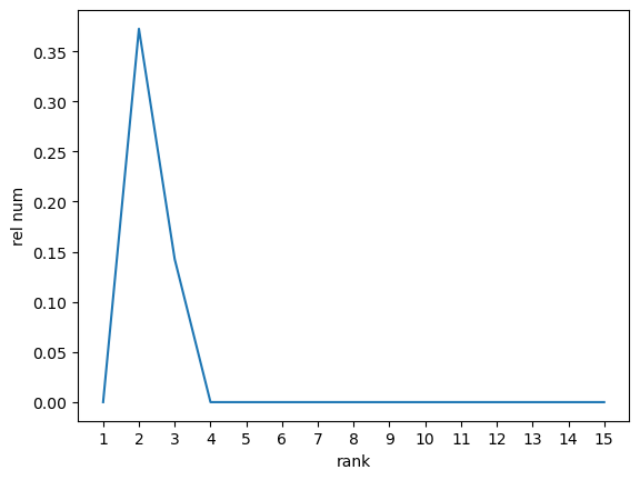
Figure 1: Number of reached cut points sorted by the rank of the tangent vector $\Delta$
(variables: $n\in\left[4,100\right]$, $p\in\left[2,15\right]$ and $\mu\in\left[2.8,3.1\right]$).

This may partly be explained by the fact that the maximum of the sectional curvature is only reached for tangent vectors of rank two and the limited range of directions for low ranks. With larger sectional curvature the boundary for cut points, respectively conjugate points, is smaller, which creates the possibility for cut points of geodesics of smaller length.
Based on this, we restrict ourselves in the following investigations to tangents with rank two. With the following observation, the space under investigation can be restricted even further. Considering the number of reached cut points on the Stiefel manifolds $St(n,p)$ in relation to the total number of examined geodesics on a Stiefel manifold we can restrict ourselves to small values for $p$ (see Figure 2). This is in line with the findings in [28].

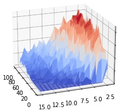
Figure 2: Number of reached cut points sorted by $n$ and $p$ (variables: $n\in\left[4,100\right]$, $p\in\left[2,15\right]$
and $\mu\in\left[2.8,3.1\right]$).

In all further investigations with $\mu\in\left[2.8,\,3.1\right]$ the smallest $\mu$ prior to which a geodesic had its cut point was found to be $2.87$. The interval is discretized in step sizes of $0.01$. To determine a more detailed statement about a bound for the injectivity radius, the shorter interval $\left[2.86,\,2.95\right]$ discretized with a step size of $0.005$ is examined (see Figure 3). Again, the smallest $\mu$ prior to which a geodesic had its cut point is $2.87$.

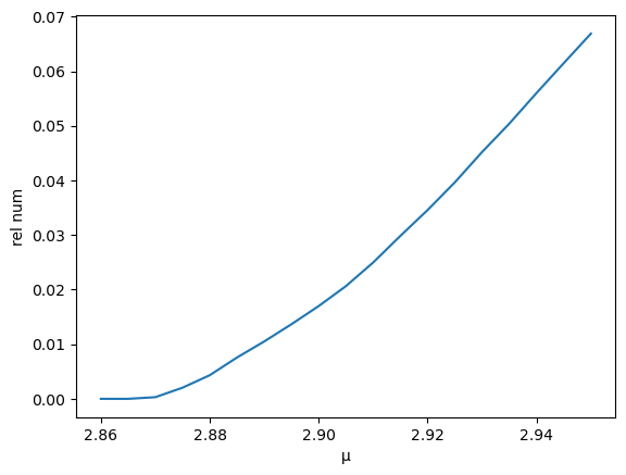
Figure 3: Number of reached cut points sorted by $\mu$ (variables: $n\in\left[4,100\right]$, $p\in\left[2,7\right]$
and $\mu\in\left[2.86,2.95\right]$ discretized in step sizes of $0.005$).

With a different approach, we further restrict the space of the analysed geodesics. From Theorem 13, we know that the bound on the injectivity radius depends on a global constant $H$ that bounds the sectional curvature on the Stiefel manifold. The larger the sectional curvature, the smaller the bound on the injectivity radius and the smaller the bound on the length of geodesics possibly having cut points, respectively. Therefore, we now restrict ourselves to the study of random geodesics with starting velocity $\Delta$ coming from a tangent plane section of maximum sectional curvature $\frac{5}{4}$. Tangent vectors spanning tangent plane sections with maximum sectional curvature can be found in [28]. Following this approach, we obtain the same results as in the previous experiments (see Figure 4).

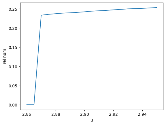
Figure 4: Number of reached cut points sorted by $\mu$ for geodesics with starting velocities from maximal sectional curvature planes (variables: $n\in\left[4,100\right]$, $p\in\left[2,7\right]$ and $\mu\in\left[2.86,2.95\right]$ discretized in step sizes of $0.005$).

For Stiefel manifolds $St(n,2)$ with $p=2$ there is another method to investigate if there are other geodesics, and, in particular, shorter geodesics to certain points. Recall Section 2.3, where it is stated that finding a geodesic connecting two points boils down to finding a suitable rotation $\Phi\in SO(p)$. Let $U_{0},\,U$ be points on the manifold (close enough to each other) and let $M=U_{0}^{T}U$ and $N=(U_{0}^{\perp})^{T}U$. Moreover, let $\left[\begin{array}[]{c}X_{0}\\ Y_{0}\end{array}\right]$ be an orthogonal completion of $\left[\begin{array}[]{c}M\\ N\end{array}\right]$ such that $\det\left(\left[\begin{array}[]{cc}M&X_{0}\\ N&Y_{0}\end{array}\right]\right)=1$. Now let $\Phi\in SO(2)$ be such that

$$\text{log}_{m}\Big{(}\underbrace{\left[\begin{array}[]{cc}M&X_{0}\Phi\\ N&Y_{0}\Phi\end{array}\right]}_{=:V_{\Phi}}\Big{)}=\left[\begin{array}[]{cc}A&-B^{T}\\ B&0\end{array}\right]$$

holds. Then $\text{Exp}_{U_{0}}(\Delta)=U$ with $\Delta=U_{0}A+QB\in T_{U_{0}}St(n,2)$. The matrices $\Phi\in SO(2)$ can be represented explicitly by

$$\Phi(\alpha)=\left[\begin{array}[]{cc}\cos(\alpha)&-\sin(\alpha)\\ \sin(\alpha)&\cos(\alpha)\end{array}\right],\qquad\text{for $\alpha\in\left[-\pi,\,\pi\right)$}.$$

Therefore, the matrix solving the geodesic endpoint problem only depends on the scalar parameter $\alpha$. We are now able to iterate over this parameter to determine $\Phi(\alpha)$ such that

$$\text{log}_{m}(V_{\Phi(\alpha)})=\left[\begin{array}[]{cc}A&-B^{T}\\ B&0\end{array}\right].$$

In this way it is possible to determine different geodesics connecting the same points (if several exist). The procedure to investigate the injectivity radius is as follows. We start with geodesics of length $3.2$. To the endpoints of this geodesic, further geodesics connecting these points are determined using the procedure described above. As soon as a shorter geodesic is found, the length of the next investigated geodesic is reduced by 0.01.

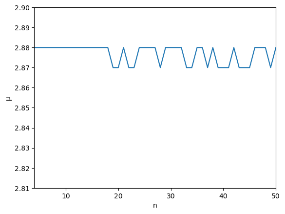
Figure 5: Smallest length $\mu$ of a geodesic to which endpoints a shorter geodesic is found
(variables: $n\in\left[4,50\right]$, $p=2$, $\mu$ started at $3.2$, stopped after $250$ iterations)

In these studies, too, the smallest length $\mu$ of geodesics to whose endpoints there are shorter geodesics is at $2.87$ (see Figure 5).
Sumarizing the numerical experiments, it was not possible to reach the theoretical bound of the injectivity radius by means of the investigation of random geodesics. Rather, the bound on the injectivity radius suggested by these experiments is around $2.87$. This coincides with the results for the canonical metric from the preprint [1] that appeared on arXiv the day before this work was submitted. In case of the canonical metric, the conjecture made by the authors of [1] is that the injectivity radius is at $\sqrt{2}t_{0}$, where $t_{0}$ is the smallest positive root of $\frac{\sin(t)}{t}+\cos(t)$. Up to 10 digits, $\sqrt{2}t_{0}=2.8690968494$. In the next Section 5, we construct an explicit example of a cut point of a geodesic at exactly this length and we find the same defining equation.

5 Explicit construction of a cut point under the canonical metric

In this section, we restrict ourselves to geodesics on the Stiefel manifold $St(4,2)$ starting in $U_{0}=\begin{bmatrix}\mathrm{I}_{2}&0\end{bmatrix}^{T}$. These are the Stiefel manifolds of smallest dimension that feature the maximum sectional curvature. Obviously, $4\times 2$-Stiefel matrices are embedded in Stiefel manifolds of larger dimensions by just filling them up with zeros in a suitable way. By Proposition 2, we know that cut points of geodesics are either first conjugate points or points to which there exist two different geodesics of equal length. Furthermore, by Remark 3, we know that the length of geodesics that feature a cut point which is no conjugate point along the geodesic is at least $\pi$. In order to determine conjugate points along a geodesic $\gamma$, we investigate Jacobi fields

$$J(t)=(d\text{Exp}_{U_{0}})_{t\gamma^{\prime}(0)}(tW)$$

along the geodesic for arbitrary directions $W\in T_{\gamma^{\prime}(0)}(T_{U_{0}}St(n,p))$. This requires us to calculate the directional derivative of the Stiefel exponential of $U_{0}$ at $t\gamma^{\prime}(0)$ in a direction $tW$. An explicit way to do this on Stiefel is outlined in [24, Section 4.2].
Let the tangent $\gamma^{\prime}(0)$ be parameterized by $A$ and $B$. Because the tangent space to a vector space can be identified with the vector space itself (see e.g. [3, p.13]), it can be argued that $T_{\gamma^{\prime}(0)}(T_{U_{0}}St(n,p))\cong T_{U_{0}}St(n,p)$. Therefore, let a direction $W\in T_{\gamma^{\prime}(0)}(T_{U_{0}}St(n,p))$ be parameterized analogous by $A_{w}$ and $B_{w}$.

According to the definition of the Stiefel exponential, the calculation of its directional derivative boils down to extracting the first two columns from the directional derivative of the matrix exponential at $t\begin{bmatrix}A&-B^{T}\\ B&0\end{bmatrix}$ in the direction $t\begin{bmatrix}A_{w}&-B_{w}^{T}\\ B_{w}&0\end{bmatrix}$. Najfeld and Havel [16] provide a formula for calculating the directional derivative of the matrix exponential. The directional derivative $D\exp_{m}(X)[Y]$ can be calculated via

$$\exp_{m}\begin{bmatrix}X&Y\\ 0&X\end{bmatrix}=\begin{bmatrix}\exp_{m}(X)&D\exp_{m}(X)[Y]\\ 0&\exp_{m}(X)\end{bmatrix}.$$ (7)

This goes by the name of Mathias’ Theorem in [11, Theorem 3.6]. The geodesic $\gamma$ that we are going to investigate is defined by $U_{0}$ and a tangent vector $\Delta$ from a tangent plane section with maximum sectional curvature. We define

$$\Delta=U_{0}\underbrace{\left[\begin{array}[]{cc}0&0\\ 0&0\end{array}\right]}_{=:A}+U_{0}^{\perp}\underbrace{\left[\begin{array}[]{cc}\frac{1}{2}&\frac{1}{2}\\ -\frac{1}{2}&\frac{1}{2}\end{array}\right]}_{=:B}.$$

By a standard result on Jacobi fields, see e. g. [6], there are $5=\text{dim}(St(4,2))$ linearly independent Jacobi fields along $\gamma$ with $J(0)=0$. Those can be found by calculating the Jacobi fields for linearly independent $w$, see [6, Chapter 5, Remark 3.2]. Five linearly independent directions $W$ defining the Jacobi fields are

$$W_{1} =U_{0}\begin{bmatrix}0&-1\\ 1&0\end{bmatrix},\quad W_{2}=U_{0}^{\perp}\begin{bmatrix}1&-1\\ 1&1\end{bmatrix},\quad W_{3}=U_{0}^{\perp}\begin{bmatrix}1&1\\ -1&1\end{bmatrix}$$

$$W_{4} =U_{0}^{\perp}\begin{bmatrix}1&1\\ 1&-1\end{bmatrix},\quad W_{5}=U_{0}^{\perp}\begin{bmatrix}-1&1\\ 1&1\end{bmatrix}.$$

Calculating the Jacobi fields via the formula for the directional derivative of the matrix exponential (7) can be done with the Jordan Canonical form. We obtain

$$J_{1}(t) =(d\text{Exp}_{U_{0}})_{t\gamma^{\prime}(0)}[tW_{1}]=\begin{bmatrix}0&-\frac{t\cos\left(\frac{t}{\sqrt{2}}\right)+\sqrt{2}\sin\left(\frac{t}{\sqrt{2}}\right)}{2}\\ \frac{t\cos\left(\frac{t}{\sqrt{2}}\right)+\sqrt{2}\sin\left(\frac{t}{\sqrt{2}}\right)}{2}&0\\ \frac{t}{2\sqrt{2}}\sin\left(\frac{t}{\sqrt{2}}\right)&-\frac{t}{2\sqrt{2}}\sin\left(\frac{t}{\sqrt{2}}\right)\\ \frac{t}{2\sqrt{2}}\sin\left(\frac{t}{\sqrt{2}}\right)&\frac{t}{2\sqrt{2}}\sin\left(\frac{t}{\sqrt{2}}\right)\end{bmatrix},$$

$$J_{2}(t) =(d\text{Exp}_{U_{0}})_{t\gamma^{\prime}(0)}[tW_{2}]=\begin{bmatrix}0&0\\ 0&0\\ \sqrt{2}\sin\left(\frac{t}{\sqrt{2}}\right)&-\sqrt{2}\sin\left(\frac{t}{\sqrt{2}}\right)\\ \sqrt{2}\sin\left(\frac{t}{\sqrt{2}}\right)&\sqrt{2}\sin\left(\frac{t}{\sqrt{2}}\right)\end{bmatrix},$$

$$J_{3}(t) =(d\text{Exp}_{U_{0}})_{t\gamma^{\prime}(0)}[tW_{3}]=\begin{bmatrix}-\sqrt{2}t\sin\left(\frac{t}{\sqrt{2}}\right)&0\\ 0&-\sqrt{2}t\sin\left(\frac{t}{\sqrt{2}}\right)\\ t\cos\left(\frac{t}{\sqrt{2}}\right)&t\cos\left(\frac{t}{\sqrt{2}}\right)\\ -t\cos\left(\frac{t}{\sqrt{2}}\right)&t\cos\left(\frac{t}{\sqrt{2}}\right)\end{bmatrix},$$

$$J_{4}(t) =(d\text{Exp}_{U_{0}})_{t\gamma^{\prime}(0)}[tW_{4}]=\begin{bmatrix}0&-\sqrt{2}t\sin\left(\frac{t}{\sqrt{2}}\right)\\ -\sqrt{2}t\sin\left(\frac{t}{\sqrt{2}}\right)&0\\ t\cos\left(\frac{t}{\sqrt{2}}\right)&t\cos\left(\frac{t}{\sqrt{2}}\right)\\ t\cos\left(\frac{t}{\sqrt{2}}\right)&-t\cos\left(\frac{t}{\sqrt{2}}\right)\end{bmatrix},$$

$$J_{5}(t) =(d\text{Exp}_{U_{0}})_{t\gamma^{\prime}(0)}[tW_{5}]=\begin{bmatrix}\sqrt{2}t\sin\left(\frac{t}{\sqrt{2}}\right)&0\\ 0&-\sqrt{2}t\sin\left(\frac{t}{\sqrt{2}}\right)\\ -t\cos\left(\frac{t}{\sqrt{2}}\right)&t\cos\left(\frac{t}{\sqrt{2}}\right)\\ t\cos\left(\frac{t}{\sqrt{2}}\right)&t\cos\left(\frac{t}{\sqrt{2}}\right)\end{bmatrix}.$$

Those Jacobi fields are linearly independent. Moreover, the matrix function values $J_{k}(t)$ at any $t$ are linearly independent as long as all $t$-dependent entries are non-zero.
There is a conjugate point that can be extracted directly from the five Jacobi fields. It is obvious that $J_{2}$ vanishes for $t=\sqrt{2}\pi$. Therefore, $\gamma$ has a conjugate point at $\sqrt{2}\pi$. Next, we investigate whether there are linear combinations of Jacobi fields that define conjugate points that are closer to $U_{0}$. Because the matrices defined by the Jacobi fields at any $t$ are linearly independent as long as all $t$-dependent entries are non-zero, we are looking for linear combinations of Jacobi fields that vanish at some $t$ where a $t$-dependent entry becomes zero. The term $\sin\left(\frac{t}{\sqrt{2}}\right)$ becomes zero for multiples of $\sqrt{2}\pi$. The term $\cos\left(\frac{t}{\sqrt{2}}\right)$ becomes zero for $\sqrt{2}\left(\frac{\pi}{2}+n\pi\right)$, $n\in\mathbb{Z}$. The smallest positive root of the term $\frac{1}{2}\left(t\cos\left(\frac{t}{\sqrt{2}}\right)+\sqrt{2}\sin\left(\frac{t}{\sqrt{2}}\right)\right)$ is $t_{1}$, where $t_{1}\approx 2.8690968494$. As the length of geodesics that feature conjugate points is bounded by the injectivity radius, the smallest candidate fulfilling $t\geq\sqrt{\frac{4}{5}}\pi$ to look for a linear combination of Jacobi fields vanishing at $t$ is $t_{1}$. In fact, $J(t)=J_{1}(t)-\frac{t_{1}}{4}J_{2}(t)$ is a Jacobi field along $\gamma$ defined by

$$W=U_{0}\begin{bmatrix}0&-1\\ 1&0\end{bmatrix}+U_{0}^{\perp}\begin{bmatrix}-\frac{t_{1}}{4}&\frac{t_{1}}{4}\\ -\frac{t_{1}}{4}&-\frac{t_{1}}{4}\end{bmatrix}$$

which vanishes at $t_{1}$. This results in $\gamma$ having its first conjugate point at $t_{1}\approx 2.8690968494$. Since the length of $\gamma$ featuring a cut point that is no conjugate point is limited to at least $\pi$, this first conjugate point $\gamma(t_{1})$ is the cut point of the geodesic $\gamma$. This example from a plane of maximal sectional curvature coincides with the observations on the injectivity radius from Section 4. In summary, we have proven

Theorem 15.

On $St(4,2)$, for arbitrary $U_{0}\in St(n,p)$, the geodesic

$$t\mapsto\gamma(t)=\text{Exp}_{U_{0}}(t\Delta),\quad\Delta=U_{0}\left[\begin{array}[]{cc}0&0\\ 0&0\end{array}\right]+U_{0}^{\perp}\left[\begin{array}[]{cc}\frac{1}{2}&\frac{1}{2}\\ -\frac{1}{2}&\frac{1}{2}\end{array}\right],$$

with starting velocity $\Delta$ from a tangent plane section of maximal sectional curvature has its cut point at its first conjugate point. This cut point occurs at the first positive root of

$$t\mapsto\left(\frac{t}{\sqrt{2}}\cos\left(\frac{t}{\sqrt{2}}\right)+\sin\left(\frac{t}{\sqrt{2}}\right)\right)$$

which is at $t_{1}\approx 2.8690968494$. As this geodesic can be embedded in all Stiefel manifolds of dimensions $p\geq 2,n\geq p+2$, the same construction gives cut points at the same geodesic length on all such $St(n,p)$.

6 Summary

This paper investigates the injectivity radius of the Stiefel manifold, which defines the size of the largest domains within which geodesics describe uniquely shortest paths everywhere on the manifold. First, we re-derive the curvature-based bound of $\sqrt{\frac{4}{5}}\pi\approx 2.81$ on the injectivity radius of the Stiefel manifold found by Rentmeesters [21]. The sharpness of this bound is an open question. We investigate the sharpness by investigating various random geodesics for their cut points numerically, which leads to bounding the injectivity radius by $2.87$ from above.
In a second part, we construct an explicit example of a cut point on the Stiefel manifold $St(4,2)$. Dimension-wise this is the first ‘true’ Stiefel manifold in the sense that the manifolds of smaller dimensions are either isomorphic to the spheres or to the orthogonal groups of corresponding dimensions. Yet, it is to be expected that all extreme cases for the injectivity radius at a point, for conjugate points or for cut points already occur here, as do the extreme cases for the sectional curvature [28].
We investigate a geodesic with starting velocity from a tangent plane section of maximal sectional curvature. For this geodesic we derive a complete, in this case five-dimensional set of linearly independent Jacobi fields along the geodesic and use them to obtain the first conjugate point along the geodesic at the smallest positive root of $\left(\frac{t}{\sqrt{2}}\cos\left(\frac{t}{\sqrt{2}}\right)+\sin\left(\frac{t}{\sqrt{2}}\right)\right)$, which is at $t_{1}\approx 2.8690968494$. This first conjugate point is describing the cut point of the geodesic and aligns with the results from the numerical experiments.
Furthermore, the results are a strong support for the conjecture made by Absil and Mataigne in [1, Conjecture 8.1] for Stiefel injectivity radius in the case of the canonical case.

The python-scripts for the numerical experiments can be found in

https://github.com/JakobStoye/StiefelInjRadius/.

Two days before the submitting this preprint, by coincidence, we learned about the work of [1] through personal communication. We would like to thank the authors of [1], Pierre-Antoine Absil and Simon Mataigne, for a very stimulating and constructive exchange at the last minute.

References

- Absil and Mataigne [2024] P. A. Absil and Simon Mataigne. The ultimate upper bound on the injectivity radius of the stiefel manifold, 2024.
- Absil et al. [2008] P.-A. Absil, R. Mahony, and R. Sepulchre. Optimization Algorithms on Matrix Manifolds. Princeton University Press, Princeton, NJ, 2008. ISBN 978-0-691-13298-3.
- Bendokat et al. [2020] Thomas Bendokat, Ralf Zimmermann, and P. A. Absil. A grassmann manifold handbook: Basic geometry and computational aspects, 2020.
- Benner et al. [2015] P. Benner, S. Gugercin, and K. Willcox. A survey of projection-based model reduction methods for parametric dynamical systems. SIAM Review, 57(4):483–531, 2015. 10.1137/130932715.
- Boumal [2023] Nicolas Boumal. An Introduction to Optimization on Smooth Manifolds. Cambridge University Press, Cambridge, 2023.
- Carmo and Flaherty [1993] Manfredo P. do Carmo and Francis Flaherty. Riemannian Geometry. Birkhäuser Boston, MA, second edition, 1993.
- Celledoni et al. [2020] E. Celledoni, S. Eidnes, B. Owren, and T. Ringholm. Mathematics of Computation, (89):699–716, 2020.
- Chakraborty and Vemuri [2018] R. Chakraborty and B. Vemuri. Statistics on the (compact) stiefel manifold: Theory and applications. The Annals of Statistics, 47, 03 2018. 10.1214/18-AOS1692.
- Edelman et al. [1998] A. Edelman, T. A. Arias, and S. T. Smith. The geometry of algorithms with orthogonality constraints. SIAM Journal on Matrix Analysis and Applications, 20(2):303–353, 1998. ISSN 0895-4798. 10.1137/S0895479895290954.
- Gallier and Quaintance [2020] J. Gallier and J. Quaintance. Differential Geometry and Lie Groups: A Computational Perspective. Geometry and Computing. Springer International Publishing, 2020. ISBN 9783030460402. https://doi.org/10.1007/978-3-030-46040-2.
- Higham [2008] N. J. Higham. Functions of Matrices: Theory and Computation. Society for Industrial and Applied Mathematics, Philadelphia, PA, USA, 2008. ISBN 978-0-898716-46-7.
- Hüper et al. [2008] K. Hüper, M. Kleinsteuber, and F. Silva Leite. Rolling Stiefel manifolds. International Journal of Systems Science, 39(9):881–887, 2008. 10.1080/00207720802184717.
- Hüper et al. [2021] K. Hüper, I. Markina, and F. Silva Leite. A Lagrangian approach to extremal curves on Stiefel manifolds. Journal of Geometrical Mechanics, 13(1):55–72, 2021.
- Lee [1997] John M. Lee. Riemannian Manifolds: An Introduction to Curvature. Graduate Texts in Mathematics. Springer New York, NY, 1997. ISBN 978-0-387-98271-7. https://doi.org/10.1007/b98852.
- Lee [2012] John M. Lee. Introduction to Smooth Manifolds. Graduate Texts in Mathematics. Springer New York, NY, 2012. ISBN 978-0-387-21752-9. https://doi.org/10.1007/978-0-387-21752-9.
- Najfeld and Havel [1995] I. Najfeld and T.F. Havel. Derivatives of the matrix exponential and their computation. Advances in Applied Mathematics, 16(3):321–375, 1995. ISSN 0196-8858. https://doi.org/10.1006/aama.1995.1017.
- Nguyen [2022] D. Nguyen. Curvatures of stiefel manifolds with deformation metrics. Journal of Lie Theory, 32(2):563–600, 2022.
- Nguyen [2021] Du Nguyen. Curvatures of stiefel manifolds with deformation metrics, 2021.
- Pennec et al. [2020] Xavier Pennec, Stefan Sommer, and Tom Fletcher, editors. Riemannian Geometric Statistics in Medical Image Analysis. Academic Press, 2020.
- Petersen [2016] P. Petersen. Riemannian Geometry. Graduate Texts in Mathematics. Springer International Publishing, 2016. ISBN 9783319266541.
- Rentmeesters [2013] Quentin Rentmeesters. Algorithms for data fitting on some common homogeneous spaces. 2013.
- Sato [2021] H. Sato. Riemannian Optimization and Its Applications. SpringerBriefs in Electrical and Computer Engineering. Springer International Publishing, 2021. ISBN 9783030623913.
- Turaga et al. [2008] P. K. Turaga, Veeraraghavan A., and R. Chellappa. Statistical analysis on Stiefel and Grassmann manifolds with applications in computer vision. In 2008 IEEE Conference on Computer Vision and Pattern Recognition, pages 1–8, June 2008. 10.1109/CVPR.2008.4587733.
- Zimmermann [2020] R. Zimmermann. Hermite interpolation and data processing errors on Riemannian matrix manifolds. SIAM Journal on Scientific Computing, 42(5):A2593–A2619, 2020. 10.1137/19M1282878.
- Zimmermann [2017] Ralf Zimmermann. A matrix-algebraic algorithm for the riemannian logarithm on the stiefel manifold under the canonical metric, 2017.
- Zimmermann [2021] Ralf Zimmermann. 7 Manifold interpolation, pages 229–274. De Gruyter, 2021. 10.1515/9783110498967-007.
- Zimmermann and Hüper [2022] Ralf Zimmermann and Knut Hüper. Computing the riemannian logarithm on the stiefel manifold: Metrics, methods, and performance. SIAM Journal on Matrix Analysis and Applications, 43(2):953–980, 2022. 10.1137/21M1425426.
- Zimmermann and Stoye [2024] Ralf Zimmermann and Jakob Stoye. High curvature means low-rank: On the sectional curvature of Grassmann and Stiefel manifolds and the underlying matrix trace inequalities, 2024.