EUROPEAN ORGANIZATION FOR NUCLEAR RESEARCH (CERN)

​​​ CERN-EP-2023-253 LHCb-PAPER-2023-036 6 March 2024

Amplitude analysis of the ${{\mathchar 28931\relax}^{0}_{b}}\!\rightarrow{p}{{K}^{-}}{\gamma}$ decay

LHCb collaboration

The resonant structure of the radiative decay ${{\mathchar 28931\relax}^{0}_{b}}\!\rightarrow{p}{{K}^{-}}{\gamma}$ in the region of proton-kaon invariant-mass up to 2.5$\text{\,Ge\kern-1.00006ptV\!/}c^{2}$ is studied using proton-proton collision data recorded at centre-of-mass energies of 7, 8, and 13  TeV collected with the LHCb detector, corresponding to a total integrated luminosity of 9$\text{\,fb}^{-1}$. Results are given in terms of fit and interference fractions between the different components contributing to this final state. Only ${\mathchar 28931\relax}$ resonances decaying to $p$ ${K}^{-}$ are found to be relevant, where the largest contributions stem from the ${\mathchar 28931\relax}(1520)$, ${\mathchar 28931\relax}(1600)$, ${\mathchar 28931\relax}(1800)$, and ${\mathchar 28931\relax}(1890)$ states.

Submitted to JHEP

© 2024 CERN for the benefit of the LHCb collaboration. CC BY 4.0 licence.

 

1 Introduction

Rare decays of $b$ hadrons involving flavour-changing neutral currents, such as ${b}\!\rightarrow{s}\ell^{+}\ell^{-}$ and ${b}\!\rightarrow{s}{\gamma}$ transitions, are forbidden at tree level in the Standard Model and further suppressed at loop-level through the GIM mechanism. As a consequence, these decays are very sensitive to potential new particles that can enter virtually through loop-level processes or allow tree-level diagrams, affecting properties of these decays such as branching fractions and angular distributions. The measurements of these processes can probe higher energy scales than those accessible via direct searches.

Thanks to the abundant production of $b$ baryons at the LHC, precision measurements of rare $b$-baryon decays have become possible for the first time. For example, the LHCb collaboration has performed tests of lepton universality using ${{\mathchar 28931\relax}^{0}_{b}}\!\rightarrow{p}{{K}^{-}}\ell^{+}\ell^{-}$ decays in the dilepton invariant-mass squared range $0.1<{q^{2}}<6.0\text{\,Ge\kern-1.00006ptV}^{2}\!/c^{4}$ and the $p$ ${K}^{-}$ invariant-mass range $m_{{p}{{K}^{-}}}<2.6\text{\,Ge\kern-1.00006ptV\!/}c^{2}$ [1]. Moreover, the LHCb collaboration has searched for $C\!P$ violation in ${{\mathchar 28931\relax}^{0}_{b}}\rightarrow{p}{{K}^{-}}\mu^{+}\mu^{-}$ decays [2] and measured the branching fraction of the ${{\mathchar 28931\relax}^{0}_{b}}\rightarrow{\mathchar 28931\relax}(1520)\mu^{+}\mu^{-}$ decay [3]. Direct interpretations of these results regarding models for physics beyond the Standard Model are difficult given the lack of detailed knowledge of the resonant structure of the $p$ ${K}^{-}$ spectrum in different regions of the dilepton invariant-mass spectrum.

An observation of the ${{\mathchar 28931\relax}^{0}_{b}}\!\rightarrow{p}{{K}^{-}}{\gamma}$ decay was first reported unofficially in a thesis using Run 1 data (taken during 2011 and 2012) without giving a significance [4]. This paper presents an amplitude analysis of the ${{\mathchar 28931\relax}^{0}_{b}}\!\rightarrow{p}{{K}^{-}}{\gamma}$ decay which constitutes the first official observation of this mode. This analysis measures ${{\mathchar 28931\relax}^{0}_{b}}\!\rightarrow{p}{{K}^{-}}{\gamma}$ decay properties for the first time and characterises the $p$ ${K}^{-}$ spectrum at the photon pole of the recoiling system. Theoretical knowledge of the $p$ ${K}^{-}$ spectrum from ${\mathchar 28931\relax}^{0}_{b}$ decays, in particular the modelling of form factors, is limited to quark-model calculations [5, 6]. Predictions obtained from lattice QCD [7, 8], HQET [9] and dispersive bounds analyses [10] are only available for the decay via the ${\mathchar 28931\relax}(1520)$ state. The different ${\mathchar 28931\relax}$ resonances in the $p$ ${K}^{-}$ spectrum have been studied using fixed target experiments with incident kaons [11, 12]. An amplitude analysis of ${{\mathchar 28931\relax}^{0}_{b}}\!\rightarrow{{J\mskip-3.0mu/\mskip-2.0mu\psi}}{p}{{K}^{-}}$ decays, which led to the discovery of states compatible with pentaquarks [13], studied the $p$ ${K}^{-}$ spectrum from ${\mathchar 28931\relax}^{0}_{b}$ decays at the ${J\mskip-3.0mu/\mskip-2.0mu\psi}$ resonance in the dimuon invariant-mass spectrum. Additionally, if the amplitudes of the ${{\mathchar 28931\relax}^{0}_{b}}\!\rightarrow{p}{{K}^{-}}{\gamma}$ decay are known precisely, this measurement could constitute useful input to a future measurement of the photon polarisation, involving polarised ${\mathchar 28931\relax}^{0}_{b}$ baryons, for example from $Z$ boson decays [14].

The ${{\mathchar 28931\relax}^{0}_{b}}\!\rightarrow{p}{{K}^{-}}{\gamma}$ decay provides an opportunity to complement the knowledge of the ${p}{{K}^{-}}$ spectrum, including unique access to heavier states with masses larger than about 2 $\text{\,Ge\kern-1.00006ptV\!/}c^{2}$ that cannot be accessed with ${{\mathchar 28931\relax}^{0}_{b}}\!\rightarrow{{J\mskip-3.0mu/\mskip-2.0mu\psi}}{p}{{K}^{-}}$ decays due to the restricted phase space. Measurements of resonance properties are vital inputs to the theoretical description of low-energy QCD as discussed in Ref. [15]. Employing data collected by the LHCb detector in $p$ $p$ collisions during the years 2011–2012 (Run 1) and 2015–2018 (Run 2), corresponding to an integrated luminosity of about 9$\text{\,fb}^{-1}$, this paper presents the first amplitude analysis of ${{\mathchar 28931\relax}^{0}_{b}}\!\rightarrow{p}{{K}^{-}}{\gamma}$ decays.

2 Detector and selection

The LHCb detector is a single-arm forward spectrometer covering the pseudorapidity range $2<\eta<5$, designed for the study of particles containing $b$ or $c$ quarks. The detector includes a high-precision tracking system consisting of a silicon-strip vertex detector surrounding the proton-proton interaction region, a large-area silicon-strip detector located upstream of a dipole magnet with a bending power of about 4 Tm, and three stations of silicon-strip detectors and straw drift tubes placed downstream of the magnet. The tracking system provides a measurement of the momentum of charged particles with a relative uncertainty that varies from 0.5% at low momentum to 1.0% at 200$\text{\,Ge\kern-1.00006ptV\!/}c$. The minimum distance of a track to a primary proton-proton collision vertex (PV), the impact parameter (IP), is measured with a resolution of $(15+29/p_{\mathrm{T}})$ $\mu$m, where $p_{\mathrm{T}}$ is the component of the momentum transverse to the beam, in $\text{\,Ge\kern-1.00006ptV\!/}c$. Different types of charged hadrons are distinguished using information from two ring-imaging Cherenkov detectors. Photons, electrons and hadrons are identified by a calorimeter system consisting of scintillating-pad (SPD) and preshower detectors, an electromagnetic (ECAL) and a hadronic calorimeter. In addition, a muon system allows the identification of muons.

Samples of simulated events are used to optimise selection requirements and estimate the efficiencies of the signal and backgrounds. The simulated proton-proton collisions are generated using Pythia [16] with a specific LHCb configuration [17]. Decays of hadronic particles are described by EvtGen [18], in which final-state radiation is generated using PHOTOS [19]. The interaction of the generated particles with the detector, and its response, are implemented in the Geant4 toolkit [20] as described in Ref. [21]. The ${{\mathchar 28931\relax}^{0}_{b}}\!\rightarrow{p}{{K}^{-}}{\gamma}$ decay is generated uniformly in phase space without assumptions on the decay dynamics.

The online event selection is performed by a trigger [22, 23], which consists of a hardware stage, based on information from the calorimeter and muon systems, followed by a software stage, which applies a full event reconstruction. The trigger exploits the presence of a high energy photon reconstructed from clusters in the ECAL. In order to reduce background and improve the mass resolution for the ${\mathchar 28931\relax}^{0}_{b}$ and two-body invariant masses, clusters are required to have a transverse energy of $E_{\mathrm{T}}>2.5$–$2.96~{}\text{\,Ge\kern-1.00006ptV}$ in Run 1 and $E_{\mathrm{T}}>2.11$–$2.7~{}\text{\,Ge\kern-1.00006ptV}$ in Run 2, respectively, at the hardware trigger level. Moreover, the hardware trigger selects only events with fewer than 600 (450) hits in the SPD for Run 1 (2) to facilitate the reconstruction in the software trigger. In the software trigger, the candidate must contain two high-$p_{\mathrm{T}}$ hadrons that are significantly displaced from the interaction point, as well as a high-$E_{\mathrm{T}}$ photon. During Run 2, a multivariate classifier based on topological criteria complements the cut-based software trigger selection [24]. The Run 1 software trigger requires the di-hadron invariant mass, assuming both hadrons are kaons, to be below 2 $\text{\,Ge\kern-1.00006ptV\!/}c^{2}$. This severely affects the shape of the efficiency as a function of the proton-kaon invariant mass, resulting in the need for separate treatment of Run 1 and Run 2. In addition to this cut in the Run 1 trigger, the large threshold for the photon energy results in low efficiency at high proton-kaon invariant mass. As a consequence, the considered phase space is reduced to a proton-kaon invariant mass of up to 2.5$\text{\,Ge\kern-1.00006ptV\!/}c^{2}$.

The reconstructed ${\mathchar 28931\relax}^{0}_{b}$ candidate is required to have good-quality track and vertex fits. Two tracks, compatible with the kaon and proton hypotheses, are required to have an impact parameter larger than $0.1~{}\text{\,mm}$, a transverse momentum larger than $1~{}\text{\,Ge\kern-1.00006ptV\!/}c$ as well as momentum larger than $5~{}\text{\,Ge\kern-1.00006ptV\!/}c$. The photon must have $E_{\mathrm{T}}>3~{}\text{\,Ge\kern-1.00006ptV}$. The ${\mathchar 28931\relax}^{0}_{b}$ decay vertex isolation is used to reject partially reconstructed backgrounds. Specifically, an upper limit is applied on the $\chi^{2}$ increase in the ${{\mathchar 28931\relax}^{0}_{b}}$ decay vertex fit when adding the most compatible additional track, referred to in the following as $\Delta\chi^{2}_{vtx}({{\mathchar 28931\relax}^{0}_{b}})$. The ${\mathchar 28931\relax}^{0}_{b}$ momentum is further required to point back to the associated primary vertex.

Background candidates resulting from combinations of unrelated protons, kaons, and photons can be suppressed using kinematic variables. A Boosted Decision Tree classifier (BDT) [25] is trained on simulated events as signal proxy and on data candidates with $m(pK\gamma)>m_{{\mathchar 28931\relax}^{0}_{b}}+300\text{\,Me\kern-1.00006ptV\!/}c^{2}$ as background proxy, to suppress combinatorial background by exploiting mainly kinematic variables. The input variables to the classifier are the momentum, pseudorapidity $\eta$, flight distance (FD), $\Delta\chi^{2}_{\rm vtx}$ of the ${\mathchar 28931\relax}^{0}_{b}$ baryon, IP and $p_{\mathrm{T}}$ of the hadrons, and IP, momentum, and $p_{\mathrm{T}}$ of the proton-kaon combination. Additionally, the difference in the vertex-fit $\chi^{2}$ of the PV associated with the ${\mathchar 28931\relax}^{0}_{b}$ baryon reconstructed with and without the ${\mathchar 28931\relax}^{0}_{b}$ candidate is used. A further input to the BDT in Run 2 is the isolation variable

$$I_{p_{\mathrm{T}}}=\frac{p_{\mathrm{T}}({{\mathchar 28931\relax}^{0}_{b}})-\sum p_{\mathrm{T}}}{p_{\mathrm{T}}({{\mathchar 28931\relax}^{0}_{b}})+\sum p_{\mathrm{T}}}$$ (1)

for which the sum is taken over tracks that are not part of the signal candidate but are associated to the same PV and fall within a cone of half-angle $\Delta R<1.7\text{\,rad}$. The half-angle of a track is defined as $(\Delta R)^{2}=(\Delta\theta)^{2}+(\Delta\phi)^{2}$, where $\Delta\theta$ and $\Delta\phi$ are the differences in the polar and azimuthal angles of each track with respect to the ${\mathchar 28931\relax}^{0}_{b}$ candidate direction. The optimal BDT working point is determined by maximising the ratio $S/\sqrt{S+B}$, where $S$ is the number of expected signal candidates estimated from simulation samples and $B$ is the number of background candidates in the signal region estimated based on the background-dominated regions on either side of the ${\mathchar 28931\relax}^{0}_{b}$ peak.

Requirements on the particle identification variables decrease backgrounds stemming from misidentification. Nevertheless, a large amount of misidentified ${{B}^{0}_{s}}\rightarrow\phi(\rightarrow{{K}^{+}}{{K}^{-}})\gamma$ decays passes all particle identification selections and pollutes the sample. These are suppressed by vetoing candidates with a ${{K}^{+}}{{K}^{-}}$ invariant mass, calculated by interpreting the proton candidate as a kaon, between $1.01$ and $1.04$$\text{\,Ge\kern-1.00006ptV\!/}c^{2}$. Remaining contributions from misidentified ${B}^{0}_{s}$ $\rightarrow$ ${K}^{-}$ ${K}^{+}$ $\gamma$ and ${B}^{0}$ $\rightarrow$ ${K}^{-}$ ${\pi}^{+}$ $\gamma$ decays are estimated to contribute less than 0.5% of the signal yield and are therefore not included in the baseline model. Background stemming from photon misidentification, such as ${{\mathchar 28931\relax}^{0}_{b}}\rightarrow p{{K}^{-}}{{\pi}^{0}}$ or ${{\mathchar 28931\relax}^{0}_{b}}\rightarrow p{{K}^{-}}\eta$, is difficult to quantify due to their unknown resonant structures. Estimates using simulation samples assuming a uniform distribution in the respective phase space indicate a contamination of 1–2% relative to the signal decay. Limiting the analysis to a proton-kaon invariant mass of 2.5$\text{\,Ge\kern-1.00006ptV\!/}c^{2}$ removes at least the contributions from potential proton-photon and kaon-photon resonances of these backgrounds which would be the most distorting. Potential contamination from ${{\mathchar 28932\relax}^{0}_{b}}\rightarrow{p}{{K}^{-}}\gamma$ decays are investigated and found to be negligible. The data are checked for remaining misidentified backgrounds by applying higher thresholds to the proton and kaon particle identification selection requirements, and by comparing different two-body invariant mass distributions under various alternative mass hypotheses. This reveals misidentified ${{D}^{0}}\rightarrow{{K}^{+}}{{K}^{-}}$ and ${{D}^{0}}\rightarrow{{K}^{+}}{{\pi}^{-}}$ decays combined with an unrelated photon, which populate the low mass side band of the signal ${\mathchar 28931\relax}^{0}_{b}$ mass peak. A veto on these decays has a strong impact on the shape of the signal acceptance in the Dalitz plane. For this reason, the candidates are retained and treated as part of the combinatorial background. The effect of this treatment is considered as a systematic uncertainty. Partially reconstructed decays, such as ${\mathchar 28931\relax}^{0}_{b}$ $\rightarrow$ $p$ ${K}^{*-}$($\rightarrow$ ${K}^{-}$ ${\pi}^{0}$)$\gamma$, where the pion is not reconstructed, are also a source of background, which is included in the fit to the three-body invariant-mass distribution described in the following.

3 Invariant mass fit

The three-body invariant mass distribution of the candidates fulfilling all selection criteria is shown in Fig. 1. An unbinned maximum-likelihood fit to these candidates is performed. Following the sPlot technique [26], a signal weight (sWeight) is assigned to each candidate to statistically disentangle the signal and background components in the subsequent amplitude analysis. The invariant mass fit is performed separately for Run 1 and Run 2, due to differences in the trigger configurations that affect the Dalitz plane distributions and hence require a separate treatment in the amplitude fit.

The signal is modelled by a double-sided Crystal-Ball [27] function comprising a Gaussian core with asymmetric tails. The tail parameters are determined using ${{\mathchar 28931\relax}^{0}_{b}}\!\rightarrow{p}{{K}^{-}}{\gamma}$ simulation samples. The remaining background due to random combinations of particles is modelled using a decreasing exponential function where the slope and yield are allowed to vary freely in the fit to data. The shape of the background from partially reconstructed decays is taken from simulation samples of ${\mathchar 28931\relax}^{0}_{b}$ $\rightarrow$ $p$ ${K}^{*-}$($\rightarrow$ ${K}^{-}$ ${\pi}^{0}$)$\gamma$ decays generated uniformly in phase space, reconstructed as signal candidates, and modelled using a kernel density estimator [28] with Gaussian kernels.

Figure 1 also shows the result of the invariant-mass fits to the Run 1 and Run 2 data sets. The signal yields are determined to be $6855\pm 93$ and $45558\pm 247$, in Run 1 and Run 2, respectively.

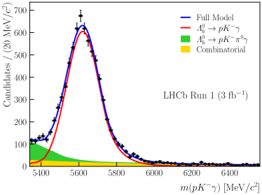
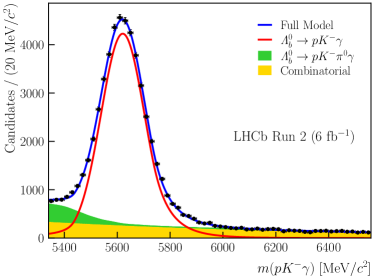
Figure 1: Distribution of the three-body invariant mass of the candidates in the (left) Run 1 and (right) Run 2 data sets. The results of the fits are overlaid.

The observed width of the ${\mathchar 28931\relax}^{0}_{b}$ mass peak is large compared to the width reconstructed using, for example, ${{\mathchar 28931\relax}^{0}_{b}}\!\rightarrow{{J\mskip-3.0mu/\mskip-2.0mu\psi}}{p}{{K}^{-}}$ decays [13]. This is a consequence of the large uncertainty in the photon momentum reconstruction, which is based on the ECAL cluster providing only limited directional information. Repeating the vertex fit while fixing the invariant mass of the ${\mathchar 28931\relax}^{0}_{b}$ candidate to the known ${\mathchar 28931\relax}^{0}_{b}$ mass value [29] reduces the uncertainty in the photon momentum for correctly identified ${{\mathchar 28931\relax}^{0}_{b}}\!\rightarrow{p}{{K}^{-}}{\gamma}$ candidates given the excellent precision of the reconstructed proton and kaon momenta [30]. The background-subtracted data in the Dalitz plane are shown in Fig. 2. The two-body invariant masses displayed here, and used in the amplitude fit later, are calculated using the ${\mathchar 28931\relax}^{0}_{b}$ mass constraint as indicated by the ${\mathchar 28931\relax}^{0}_{b}$ subscript.

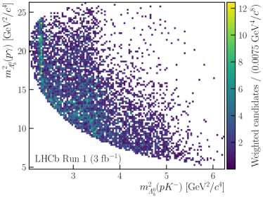
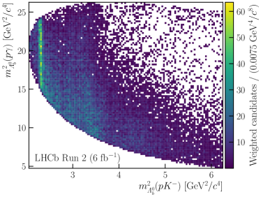
Figure 2: Distribution of the ${{\mathchar 28931\relax}^{0}_{b}}\!\rightarrow{p}{{K}^{-}}{\gamma}$ candidates in the Dalitz plane, defined by $m^{2}_{{\mathchar 28931\relax}^{0}_{b}}({p}{{K}^{-}})$ and $m^{2}_{{\mathchar 28931\relax}^{0}_{b}}(p\gamma)$, after background-subtraction using the sPlot method for (left) Run 1 and (right) Run 2.

As a cross-check for the combination of data within a single run period, the fit to the three-body invariant mass is performed on the full data set and the data set of each year individually. No significant discrepancies between the fit results are observed. In order to validate the sPlot technique, fits to the three-body invariant mass are also performed in bins of the proton-kaon and the proton-photon invariant masses; these fits yield compatible results.

4 Amplitude model

The structures in the data shown in Fig. 2 are described using an amplitude model following the prescription of Ref. [31]. The intermediate ${\mathchar 28931\relax}$ resonances decaying to $p{{K}^{-}}$ are modelled assuming Breit–Wigner lineshapes, while their spin-dependent angular distributions are described by the helicity formalism.

The three-body decay of a particle with non-zero spin results in five independent phase-space dimensions. Given that the ${\mathchar 28931\relax}^{0}_{b}$ baryons observed by LHCb are produced unpolarised [32], the dimensionality of the phase space relevant to this analysis is reduced from five to two [31]. In the following, the phase-space position is denoted $\mathcal{D}$. This position can be expressed in terms of the Dalitz variables [33] as shown in Fig. 2 for the background-subtracted data. Equivalently, the phase-space position can be given by the proton-kaon invariant mass, $m(p{{K}^{-}})$ and the cosine of the proton helicity angle, $\cos\theta_{p}$, as is used in Ref. [34]. The helicity angle of the proton, $\theta_{p}$, is the polar angle of the proton momentum in the proton-kaon rest frame where the $z$ axis coincides with the $\mathchar 28931\relax$ resonance polarisation axis. This angle can be calculated using two steps. First, the proton and resonance momentum are boosted into the ${\mathchar 28931\relax}^{0}_{b}$ rest frame where the coordinate system is defined such that the resonance momentum direction coincides with the $z$ axis. Second, the proton momentum is boosted into the proton-kaon rest frame. The magnitude of the $z$ component of the obtained proton momentum, $\vec{p}$, defines the cosine of the proton helicity angle

$$\cos\theta_{p}=\frac{p_{z}}{\mid\vec{p}\mid}\ .$$ (2)

The amplitude of the decay chain ${{\mathchar 28931\relax}^{0}_{b}}\rightarrow{\mathchar 28931\relax}(\rightarrow p{{K}^{-}}){\gamma}$ with resonance spin $J_{\mathchar 28931\relax}$ and particle helicities denoted by $\lambda_{i}$ is

$$\mathcal{A}^{\mathchar 28931\relax}_{\lambda_{\gamma},\lambda_{\mathchar 28931\relax},\lambda_{p}}=d^{J_{\mathchar 28931\relax}}_{\lambda_{\mathchar 28931\relax}\lambda_{p}}(\theta_{p})H_{\lambda_{\mathchar 28931\relax},\lambda_{\gamma}}^{{\mathchar 28931\relax}}h_{\lambda_{p}}^{{\mathchar 28931\relax}}X_{J_{\mathchar 28931\relax}}\left(m(p{{K}^{-}})\right)\ .$$ (3)

The function $X_{J_{\mathchar 28931\relax}}\left(m(p{{K}^{-}})\right)$ represents the resonance dynamics. The Wigner $d$-matrix elements, $d^{J_{\mathchar 28931\relax}}_{\lambda_{\mathchar 28931\relax}\lambda_{p}}(\theta_{p})$ [35], describe the rotation of spin states from the ${\mathchar 28931\relax}$ helicity frame into the proton helicity frame. The helicity-coupling amplitudes $H$ and $h$ contain the information about the dynamics of the decays ${{\mathchar 28931\relax}^{0}_{b}}\!\rightarrow{\mathchar 28931\relax}{\gamma}$ and ${\mathchar 28931\relax}\!\rightarrow{p}{{K}^{-}}$, respectively. Given that the kaon has spin-0, its helicity is also zero and is omitted in the index of the ${\mathchar 28931\relax}\!\rightarrow{p}{{K}^{-}}$ helicity amplitude, $h$.

Helicity conservation, defined as $\lambda_{b}=\lambda_{\mathchar 28931\relax}-\lambda_{\gamma}$, must be fulfilled. As a result, the resonance helicities can only take the values $\lambda_{\mathchar 28931\relax}=\pm\tfrac{1}{2}$ for $J_{\mathchar 28931\relax}=\pm\tfrac{1}{2}$ and $\lambda_{\mathchar 28931\relax}=\pm\tfrac{1}{2},\pm\tfrac{3}{2}$ for $J_{\mathchar 28931\relax}\geq\tfrac{3}{2}$. Moreover, the resonance and photon helicities must have the same sign. Subsequently, there are two (four) helicity couplings for each resonance with spin-$\tfrac{1}{2}$ ($\geq\tfrac{3}{2}$). Standard parametrisations of resonance dynamics depend on the orbital angular momentum between the children in a decay requiring a transformation of Eq. (3) from the helicity to the canonical basis

$$\begin{split}\mathcal{A}^{\mathchar 28931\relax}_{\lambda_{\gamma},\lambda_{\mathchar 28931\relax},\lambda_{p}}=d^{J_{\mathchar 28931\relax}}_{\lambda_{\mathchar 28931\relax}\lambda_{p}}(\theta_{p})&\sum_{l=|J_{\mathchar 28931\relax}-s|}^{|J_{\mathchar 28931\relax}+s|}\sum_{s=|J_{p}-J_{K}|}^{|J_{p}+J_{K}|}C^{\mathchar 28931\relax}_{ls}h^{{\mathchar 28931\relax}}_{ls}\\ \times&\sum_{L=|J_{b}-S|}^{|J_{b}+S|}\sum_{S=|J_{\mathchar 28931\relax}-J_{\gamma}|}^{|J_{\mathchar 28931\relax}+J_{\gamma}|}C^{\mathchar 28931\relax}_{LS}H^{{\mathchar 28931\relax}}_{LS}X_{Ll}^{\mathchar 28931\relax}\left(m(p{{K}^{-}}\right))\ ,\end{split}$$ (4)

where the angular dependence remains unchanged. This transformation couples the spins of the child particles in a decay to a total spin which is then coupled with their orbital angular momentum. The factors $C^{\mathchar 28931\relax}_{LS}$ and $C^{\mathchar 28931\relax}_{ls}$ are the products of the Clebsch-Gordan coefficients required in the spin-spin and spin-orbital-angular-momentum coupling for the resonance-photon and proton-kaon systems, respectively. In the resonance-photon system, the total spin, $S$, and orbital angular momentum, $L$, can take different values such that the product of the Clebsch-Gordan coefficients is

$$C^{\mathchar 28931\relax}_{LS}=\sqrt{\frac{2L+1}{2J_{b}+1}}\langle J_{\mathchar 28931\relax},\lambda_{\mathchar 28931\relax};J_{\gamma},-\lambda_{\gamma}|S,(\lambda_{\mathchar 28931\relax}-\lambda_{\gamma})\rangle\cdot\langle L,0;S,(\lambda_{\mathchar 28931\relax}-\lambda_{\gamma})|J_{b},\lambda_{b}\rangle\ .$$ (5)

The total spin of the $p{{K}^{-}}$ system is $s=\tfrac{1}{2}$, as the kaon carries no spin. The orbital angular momentum between the proton and the kaon, $l$, is fixed for a given spin-parity combination due to angular momentum and parity conservation in the strong decay ${\mathchar 28931\relax}\!\rightarrow{p}{{K}^{-}}$. The corresponding Clebsch-Gordan coefficients in the proton-kaon system are

$$C^{\mathchar 28931\relax}_{ls}=1\cdot\langle l,0;J_{p},\lambda_{p}|J_{\mathchar 28931\relax},\lambda_{p}\rangle\ .$$ (6)

Hence, the summation over the spin and orbital angular momentum of the $p{{K}^{-}}$ system can be dropped and only one coupling $h^{{\mathchar 28931\relax}}_{ls}$ remains and is absorbed into the $H_{LS}^{{\mathchar 28931\relax}}$ couplings:

$$A_{LS}^{\mathchar 28931\relax}=H^{{\mathchar 28931\relax}}_{LS}h^{{\mathchar 28931\relax}}_{ls}\ .$$ (7)

A standard parametrisation of resonance dynamics as employed in previous amplitude analyses (for example in Refs. [13, 36]) is used:

$$X_{Ll}^{\mathchar 28931\relax}(m)=\underbrace{\left(\frac{|\vec{q}|}{q_{0}}\right)^{L}B_{L}(|\vec{q}|,q_{0})}_{{{\mathchar 28931\relax}^{0}_{b}}\!\rightarrow{\mathchar 28931\relax}{\gamma}}\underbrace{\left(\frac{|\vec{p}|}{p_{0}}\right)^{l}B_{l}(|\vec{p}|,p_{0})}_{{\mathchar 28931\relax}\!\rightarrow{p}{{K}^{-}}}\text{BW}(m)\ ,$$ (8)

where $\vec{q}$ ($\vec{p}$) is the momentum of the resonance (proton) in the ${\mathchar 28931\relax}^{0}_{b}$ (${\mathchar 28931\relax}$) rest frame and $B_{l}$ and $B_{L}$ are Blatt–Weisskopf form factors [37]. Accordingly, the magnitudes of the momenta at the nominal resonance mass are $q_{0}$ and $p_{0}$. The resonance is modelled using a Breit–Wigner (BW) distribution [38]

$$\text{BW}(m)=\frac{1}{m_{0}^{2}-m^{2}-im_{0}\Gamma(m)}\ ,\quad\Gamma(m)=\Gamma_{0}\left(\frac{p}{p_{0}}\right)^{2l+1}\frac{m_{0}}{m}\left[B_{l}(p,p_{0})\right]^{2}\ ,$$ (9)

with resonance mass $m_{0}$ and width $\Gamma_{0}$. For the ${\mathchar 28931\relax}(1405)$ resonance, with a pole-mass below the $p$ ${K}^{-}$ threshold, a similar approach as the amplitude analyses of ${{\mathchar 28931\relax}^{0}_{b}}\!\rightarrow{{J\mskip-3.0mu/\mskip-2.0mu\psi}}{p}{{K}^{-}}$ [13] and ${{\mathchar 28931\relax}^{+}_{c}}\rightarrow{p}{{K}^{-}}{{\pi}^{+}}$ [39] is employed, i.e. using a two-component width equivalent to the Flatté parametrisation [40]. The barrier factors, $(|\vec{q}|/m_{{\mathchar 28931\relax}^{0}_{b}})^{L}$ and $(|\vec{p}|/m_{0})^{l}$, suppress high orbital angular momenta compared to low ones, which will be exploited to simplify the model later on. The Blatt–Weisskopf form factors are equal to one at the resonance pole and shape the resonance peak depending on the orbital angular momentum. This analysis uses the same parametrisation of the Blatt–Weisskopf functions as Ref. [13]. Following the choice made in Ref. [36], the radius of the ${\mathchar 28931\relax}^{0}_{b}$ baryon is taken to be $5~{}(\!\text{\,Ge\kern-1.00006ptV}/(c\hbar))^{-1}$ and the radius of the $\mathchar 28931\relax$ resonances is taken to be $1.5~{}(\!\text{\,Ge\kern-1.00006ptV}/(c\hbar))^{-1}$.

The final decay rate is the sum over all appearing ${\mathchar 28931\relax}$ resonances and their possible helicities, $\lambda_{\mathchar 28931\relax}$, as well as the initial and final state helicities, $\lambda_{b},\lambda_{\gamma},\lambda_{p}$

$$\begin{split}\frac{\mathrm{d}\Gamma}{\mathrm{d}\mathcal{D}}=\frac{1}{2}\sum_{\lambda_{b},\lambda_{\gamma},\lambda_{p}}&\left|\sum_{{\mathchar 28931\relax}}\sum_{\lambda_{\mathchar 28931\relax}}d^{J_{\mathchar 28931\relax}}_{\lambda_{\mathchar 28931\relax}\lambda_{p}}(\theta_{p})C^{\mathchar 28931\relax}_{ls}\sum_{L=|J_{b}-S|}^{|J_{b}+S|}\sum_{S=|J_{\mathchar 28931\relax}-J_{\gamma}|}^{|J_{\mathchar 28931\relax}+J_{\gamma}|}C^{\mathchar 28931\relax}_{LS}A^{{\mathchar 28931\relax}}_{LS}X_{Ll}^{\mathchar 28931\relax}\left(m(p{{K}^{-}})\right)\right|^{2}\ .\end{split}$$ (10)

The decay is assumed to be $C\!P$-conserving such that the amplitudes of the decay ${{\mathchar 28931\relax}^{0}_{b}}\rightarrow p{{K}^{-}}{\gamma}$ and ${{\kern 1.79993pt\overline{\kern-1.79993pt\mathchar 28931\relax}}{}^{0}_{b}}\rightarrow{\overline{p}}{{K}^{+}}{\gamma}$ have the same helicity couplings. As a consequence of isospin suppression, investigated experimentally in Ref. [41] and theoretically in Ref. [42], the ${{\mathchar 28931\relax}^{0}_{b}}\!\rightarrow{p}{{K}^{-}}{\gamma}$ decay is dominated by the ${\mathchar 28931\relax}$ states and therefore $\mathchar 28934\relax$ resonances, which have the same quark content but different isospin, are not considered in this analysis. Additionally, resonances in the proton-photon and kaon-photon invariant masses are not included as they almost exclusively populate the phase space at $m(pK)>2.5$$\text{\,Ge\kern-1.00006ptV\!/}c^{2}$.

Besides resonances, additional nonresonant components may be necessary to achieve a satisfactory description of the data. Such nonresonant contributions are modelled similarly to the resonances, where the Breit–Wigner peak is replaced by an exponential function or a constant

$$\begin{split}X_{Ll}^{\text{NR,exp}}(m)&=\underbrace{\left(\frac{|\vec{q}|}{q_{0}}\right)^{L}\left(\frac{|\vec{p}|}{p_{0}}\right)^{l}}_{\text{barrier factors}}\exp\left(-\alpha(m^{2}-m_{\text{NR}}^{2})\right)\,,\\ X_{Ll}^{\text{NR,const}}(m)&=\underbrace{\left(\frac{|\vec{q}|}{q_{0}}\right)^{L}\left(\frac{|\vec{p}|}{p_{0}}\right)^{l}}_{\text{barrier factors}}\,.\end{split}$$ (11)

The mass parameter used in the computation of $p_{0}$ and $q_{0}$ of the nonresonant component is set to the centre of the possible proton-kaon invariant-mass range: $m_{\text{NR}}=3.5\text{\,Ge\kern-1.00006ptV\!/}c^{2}$. The parameter $\alpha$ is determined by the fit. To incorporate this into the decay rate, the sum over all resonances in Eq. (10) needs to include the nonresonant component. The corresponding coherent sum over the helicity states resembles the sum of a resonant contribution where only the lineshape in Eq. (8) is replaced by the one in Eq. (11).

Finally, the transformation into the $LS$ basis must conserve the number of degrees of freedom (two (four) helicity couplings for each ${\mathchar 28931\relax}$ with spin $\tfrac{1}{2}$ ($\geq\tfrac{3}{2}$)). However, given that the angular momentum coupling is a purely mathematical transformation and lacks physics knowledge such as $\lambda_{\gamma}\not=0$, there are four (six) $LS$ combinations for spin $\tfrac{1}{2}$ ($\geq\tfrac{3}{2}$) resonances. Translating $H_{\pm 1/2,0}=0$ into a combination of $LS$ couplings is non trivial. An approximation omitting all dynamical terms in Eq. (4) is obtained by expressing the two couplings with highest $S$ in terms of the other two or four:

$$\begin{split}\begin{pmatrix}A_{L_{\text{max}},S_{\text{max}}}^{{\mathchar 28931\relax}}\\ A_{L_{\text{max}}-1,S_{\text{max}}}^{{\mathchar 28931\relax}}\end{pmatrix}=-\begin{pmatrix}C^{+}_{L_{\text{max}},S_{\text{max}}}&C^{+}_{L_{\text{max}}-1,S_{\text{max}}}\\ C^{-}_{L_{\text{max}},S_{\text{max}}}&C^{-}_{L_{\text{max}}-1,S_{\text{max}}}\end{pmatrix}^{-1}\sum_{L,S<S_{\text{max}}}A_{L,S}^{{\mathchar 28931\relax}}\begin{pmatrix}C_{LS}^{+}\\ C_{LS}^{-}\end{pmatrix}\ .\end{split}$$ (12)

The constants $C_{LS}^{\pm}$ are the Clebsch-Gordan coefficients $C_{LS}^{{\mathchar 28931\relax}}$ with resonance helicity $\lambda_{\mathchar 28931\relax}=\pm\tfrac{1}{2}$ and photon helicity $\lambda_{\gamma}=0$. In the case of a spin-$\tfrac{3}{2}$ resonance for example, there are six $LS$ combinations: $(0,\tfrac{1}{2}),(1,\tfrac{1}{2}),(1,\tfrac{3}{2}),(2,\tfrac{3}{2}),(2,\tfrac{5}{2}),(3,\tfrac{5}{2})$. The transformation in Eq. (12) replaces the latter two and ensures that the amplitude vanishes exactly at the nominal mass of the resonance.

Two interesting quantities that can be extracted from the model are the fit fraction, the relative contribution of a single resonance to the determined full amplitude computed by

$$\text{FF}(n)=\frac{\int_{\mathcal{D}}\left(\frac{\mathrm{d}\Gamma(n)}{\mathrm{d}\mathcal{D}}\right)\mathrm{d}\mathcal{D}}{\int_{\mathcal{D}}\left(\frac{\mathrm{d}\Gamma}{\mathrm{d}\mathcal{D}}\right)\mathrm{d}\mathcal{D}}\ ,$$ (13)

and the interference fit fraction

$$\text{IFF}(n,m)=\frac{\int_{\mathcal{D}}\left(\frac{\mathrm{d}\Gamma(n,m)}{\mathrm{d}\mathcal{D}}\right)\mathrm{d}\mathcal{D}}{\int_{\mathcal{D}}\left(\frac{\mathrm{d}\Gamma}{\mathrm{d}\mathcal{D}}\right)\mathrm{d}\mathcal{D}}-\text{FF}(n)-\text{FF}(m)\ .$$ (14)

Here, $\mathrm{d}\Gamma(n)/\mathrm{d}\mathcal{D}$ is the decay rate for a single state $n$, i.e. where the sum in Eq. (10) only contains the state $n$. Similarly, $\mathrm{d}\Gamma(n,m)/\mathrm{d}\mathcal{D}$ is the decay rate of two states $n,m$, i.e. where the sum in Eq. (10) only contains the states $n$ and $m$. In contrast, $\mathrm{d}\Gamma/\mathrm{d}\mathcal{D}$ is the decay rate containing all states of a given model.

5 Amplitude fit

A simultaneous, unbinned, maximum-likelihood fit of the amplitude model to the Run 1 and Run 2 data sets determines the $LS$ couplings $A_{LS}$. The negative logarithm of the likelihood function (NLL) is defined as [43]

$$\text{NLL}\equiv-\log(\mathcal{L})= -\sum_{\text{Run 1}}\log\left(f_{1}\left(\mathcal{D}\right)\right)w_{s}-\sum_{\text{Run 2}}\log\left(f_{2}\left(\mathcal{D}\right)\right)w_{s}\ .$$ (15)

The weights $w_{s}$ are the sPlot weights presented in Sec. 3 normalised to the effective sample size [44]. The probability distribution functions $f_{i}$ correspond to the normalised rate in Eq. (10), multiplied by the efficiency map $\varepsilon_{i}(\mathcal{D})$ of Run 1 or Run 2:

$$f_{i}(\mathcal{D})=\frac{\varepsilon_{i}(\mathcal{D})}{I_{i}}\frac{\mathrm{d}\Gamma}{\mathrm{d}\mathcal{D}}\ ,$$ (16)

where the normalisation factor is calculated as

$$I_{i}=\int_{\mathcal{D}}\varepsilon_{i}(\mathcal{D})\frac{\mathrm{d}\Gamma}{\mathrm{d}\mathcal{D}}\mathrm{d}\mathcal{D}\ .$$ (17)

The efficiency maps, obtained from simulation samples, are implemented as interpolated histograms. The fit is performed using the TensorFlowAnalysis package [45].

Table 1 lists all ${\mathchar 28931\relax}$ resonances whose existence ranges from very likely to certain according to Ref. [29]. Such states are rated three or four stars and are derived from analyses of data sets that include precision differential cross sections and polarisation observables, and are confirmed by independent analyses. The allowed values of the orbital angular momenta between the proton and the kaon, $l$, and the resonance and the photon, $L$, are given explicitly in the rightmost columns.

Table 1: List of well-established ${\mathchar 28931\relax}$ resonances and their properties as given in Ref. [29]. $J$ and $P$ are spin and parity of the resonance. The mass $m_{0}$ and width $\Gamma_{0}$ correspond to the Breit–Wigner parameters and are given in $\text{\,Me\kern-1.00006ptV\!/}c^{2}$ and  MeV respectively. The possible mass and width ranges, $\Delta m_{0}$ and $\Delta\Gamma_{0}$, are also given. If a measurement of mass and width is available, the uncertainties are given instead of a range. The columns $\sigma_{m_{0}}$ and $\sigma_{\Gamma_{0}}$ contain the $\sigma$ values used to estimate the systematic uncertainty related to the resonance parameters. The rightmost columns contain the allowed values of $l$ and $L$.

Resonance	$J^{P}$	$m_{0}$	$\Gamma_{0}$	$\Delta m_{0}$	$\Delta\Gamma_{0}$	$\sigma_{m_{0}}$	$\sigma_{\Gamma_{0}}$	$l$	$L$
${\mathchar 28931\relax}(1405)$	$\nicefrac{{1}}{{2}}^{-}$	1405	50.5	$\pm 1.3$	$\pm 2$	1.3	2	0	0, 1
${\mathchar 28931\relax}(1520)$	$\nicefrac{{3}}{{2}}^{-}$	1519	16	1518 – 1520	115 – 117	1	1	2	0, 1, 2
${\mathchar 28931\relax}(1600)$	$\nicefrac{{1}}{{2}}^{+}$	1600	200	1570 – 1630	150 – 250	30	50	1	0, 1
${\mathchar 28931\relax}(1670)$	$\nicefrac{{1}}{{2}}^{-}$	1674	30	1670 – 1678	125 – 135	4	5	0	0, 1
${\mathchar 28931\relax}(1690)$	$\nicefrac{{3}}{{2}}^{-}$	1690	70	1685 – 1695	150 – 170	5	10	2	0, 1, 2
${\mathchar 28931\relax}(1800)$	$\nicefrac{{1}}{{2}}^{-}$	1800	200	1750 – 1850	150 – 250	50	50	0	0, 1
${\mathchar 28931\relax}(1810)$	$\nicefrac{{1}}{{2}}^{+}$	1790	110	1740 – 1840	150 – 170	50	60	1	0, 1
${\mathchar 28931\relax}(1820)$	$\nicefrac{{5}}{{2}}^{+}$	1820	80	1815 – 1825	170 – 190	5	10	3	1, 2, 3
${\mathchar 28931\relax}(1830)$	$\nicefrac{{5}}{{2}}^{-}$	1825	90	1820 – 1830	160 – 120	5	30	2	1, 2, 3
${\mathchar 28931\relax}(1890)$	$\nicefrac{{3}}{{2}}^{+}$	1890	120	1870 – 1910	180 – 160	20	40	1	0, 1, 2
${\mathchar 28931\relax}(2100)$	$\nicefrac{{7}}{{2}}^{-}$	2100	200	2090 – 2110	100 – 250	10	100	4	2, 3, 4
${\mathchar 28931\relax}(2110)$	$\nicefrac{{5}}{{2}}^{+}$	2090	250	2050 – 2130	200 – 300	40	50	3	1, 2, 3
${\mathchar 28931\relax}(2350)$	$\nicefrac{{9}}{{2}}^{+}$	2350	150	2340 – 2370	100 – 250	20	100	5	3, 4, 5

The fit parameters are the couplings $A^{\mathchar 28931\relax}_{LS}$, resulting in 45 independent complex variables when including all listed ${\mathchar 28931\relax}$ resonances. A baseline fit comprising these contributions determines ${\mathchar 28931\relax}(1800)$ as the largest component. To fix the overall phase and magnitude of the full amplitude, its coupling with lowest $L$ is therefore set to $|A^{1800}_{0,1/2}|=1$ and $\arg(A^{1800}_{0,1/2})=0$.

Due to the complexity of the amplitude model, the NLL function has many local minima. Depending on the exact combination of initial values, the fit may converge to different minima. When determining the best model, the fit is repeated ten times starting from randomised initial values. Only the result with the lowest NLL out of these ten is compared to the other models. This procedure reduces the risk of choosing the wrong best model based on convergence to a local minimum. While the different minima correspond to different values of the couplings, the values for the fit fractions and interference fit fractions are similar for different minima. As a result of this instability with respect to the couplings, this analysis treats them as nuisance parameters while the derived fit fractions and interference fit fractions are the observables.

The quality of the fit is determined using a binned $\chi^{2}$ test comparing the two-dimensional weighted data histogram in ($m_{{{\mathchar 28931\relax}^{0}_{b}}}({p}{{K}^{-}}),\cos\theta_{p}$) with the fit result. The latter is obtained by generating a large sample of 6$\times 10^{6}$ data points — more than 100 times the combined signal yield — from the fitted pdf. Because some regions of the phase space are only sparsely populated, the histogram is defined using a non-uniform binning with at least 100 observed signal events in each bin. Due to the differences in the Run 1 and Run 2 acceptance shapes, this binning is calculated separately for the two subsets.

The initial model contains all well-known ${\mathchar 28931\relax}$ resonances (see Table 1) and no other components. This gives an good description of the major structures in the data. This model is referred to as the reduced model. The distribution of the proton-kaon invariant-mass in Run 1 and Run 2 is shown in Fig. 3. The projection of the reduced model including all its components is overlaid. While the reduced model overall describes the data spectrum well, the model is not satisfactory in the region $m_{{{\mathchar 28931\relax}^{0}_{b}}}({p}{{K}^{-}})>2\text{\,Ge\kern-1.00006ptV\!/}c^{2}$. As the heavy ${\mathchar 28931\relax}$ states are poorly known, the mass and width of different combinations of heavy states are floated with Gaussian constraints of $100\text{\,Me\kern-1.00006ptV\!/}c^{2}$ around the values obtained from Ref. [29] in order to improve the fit quality. Allowing the mass and width of the ${\mathchar 28931\relax}(2100)$ and ${\mathchar 28931\relax}(2110)$ states to vary, while keeping those of the ${\mathchar 28931\relax}(2350)$ state fixed, yields the biggest improvement.

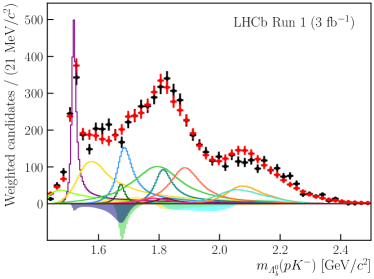
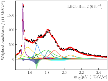
Figure 3: Background-subtracted distribution of the proton-kaon invariant-mass (black dots) for the (left) Run 1 and (right) Run 2 data samples. Also shown is a sample generated according to the result of a simultaneous fit of the reduced model to the data (red dots) and its components (lines) as well as the contributions due to interference between states with the same quantum numbers $J^{P}$ (shaded areas).

Another option to improve the fit quality is the addition of nonresonant contributions. The nonresonant components can affect the entire region of the phase space, and are especially important in regions where resonances with the matching spin-parity may interfere. Nonresonant components with spins up to $\tfrac{5}{2}$ and both parities, using an exponential or constant lineshape (see Eq. 11), are tested. Both lineshape functions tested yield very similar results for a given set of quantum numbers and the constant one is taken as the default lineshape. The model including a nonresonant component with quantum numbers $J^{P}=\tfrac{3}{2}^{-}$ results in the best fit quality for either lineshape. The fit quality of this model is better than the fit quality of the reduced model with floating resonance masses and widths.

As a result, the best model used to determine the default result consists of the reduced model containing all ${\mathchar 28931\relax}$ states with mass and width fixed to the values given in Table 1 and a nonresonant component with quantum numbers $J^{P}=\tfrac{3}{2}^{-}$. Figures 4 and 5 contain projections of the data and the model with its components onto all two-body invariant masses as well as the proton helicity angle for Run 1 and Run 2. Appendix A shows the projections onto the proton-kaon invariant mass using a logarithmic vertical axis. The same set of plots is provided in Appendix B for the fit with floating resonances representing the second best model.

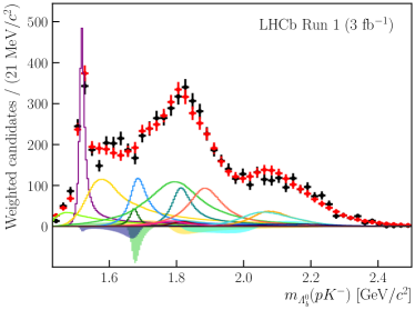
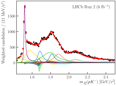
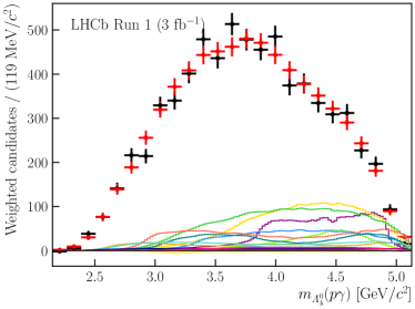
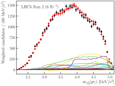
Figure 4: Background-subtracted distribution of the (top) proton-kaon and (bottom) proton-photon invariant-mass (black dots) for the (left) Run 1 and (right) Run 2 data samples. Also shown is a sample generated according to the result of a simultaneous fit of the default model to the data (red dots) and its components (lines) as well as the contributions due to interference between states with the same quantum numbers $J^{P}$ (shaded areas).

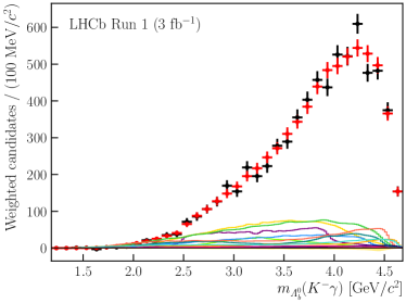
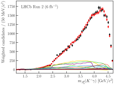
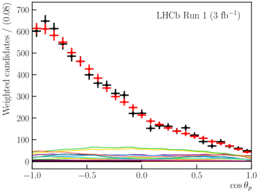
Figure 5: Background-subtracted distribution of (top) the kaon-photon invariant-mass and (bottom) the proton helicity angle (black dots) for the (left) Run 1 and (right) Run 2 data samples. Also shown is a sample generated according to the result of a simultaneous fit of the default model to the data (red dots) and its components (lines) as well as the contributions due to interference between states with the same quantum numbers $J^{P}$ (shaded areas). See Fig. 4 for the legend.

The statistical uncertainties on the fit fractions and interference fit fractions are determined by bootstrapping the data 250 times. This means that the data set is resampled and a new set of sWeights is calculated from a fit to the three-body invariant mass of each bootstrap sample. Running the amplitude fit on each sample with its respective sWeights results in a distribution for each observable. The value for the statistical confidence interval given later is obtained by finding the shortest 68% interval around the maximum of this distribution.

6 Systematic uncertainties

Systematic uncertainties arise from four major categories: the choice of amplitude model, the acceptance model, the invariant-mass fit model, and potential remaining backgrounds. The individual uncertainties are listed in Table 2 and outlined in the following.

6.1 Amplitude model

In the default fit, the masses and widths of the resonances are set to their world averages and fixed in the fit. To assess the impact of this choice, alternative masses and widths are sampled from Gaussian distributions. The widths of the Gaussians are given in Table 1 as $\sigma_{m_{0}}$ and $\sigma_{\Gamma_{0}}$ and are chosen based on the ranges $\Delta m_{0}$ and $\Delta\Gamma_{0}$. Pseudoexperiments, generated using these alternative mass and width values, are fitted with the default model. The shortest 68% interval around the maximum of the distribution of the difference between the generated and fitted values is taken as a systematic uncertainty.

Similar to the treatment of the masses and widths, also the ${\mathchar 28931\relax}^{0}_{b}$ and $\mathchar 28931\relax$ radii used in the Blatt–Weisskopf functions are fixed to $d_{{\mathchar 28931\relax}^{0}_{b}}=5~{}(\text{\,Ge\kern-1.00006ptV}/(c\hbar))^{-1}$ and $d_{\mathchar 28931\relax}=1.5~{}(\text{\,Ge\kern-1.00006ptV}/(c\hbar))^{-1}$ in the default fit. The impact of this choice is assessed by generating samples with $d_{{\mathchar 28931\relax}^{0}_{b}}=3,5,7~{}(\!\text{\,Ge\kern-1.00006ptV}/(c\hbar))^{-1}$ and $d_{\mathchar 28931\relax}=0.5,1.5,2.5,3.5$ and $4.5~{}(\!\text{\,Ge\kern-1.00006ptV}/(c\hbar))^{-1}$. These samples are fitted with the default model. The bias and standard deviation of the differences between the generated and fitted values for each combination of $d_{{\mathchar 28931\relax}^{0}_{b}}$ and $d_{\mathchar 28931\relax}$ is taken as systematic uncertainty.

Table 2: Systematic uncertainties on the fit fractions (top part of the table) and interference fit fractions (bottom part of the table). The values are given in %. The subscripts “BW”, “radius”, “amp.”, and “res.” refer to the systematic uncertainty due to fixing the resonance mass and width, fixing the radius of the hadrons, the choice of amplitude model, and the neglected resolution in the amplitude fit, respectively. The subscripts “finite”, “acc.”, and “kin.” refer to the systematic uncertainties due to the finite simulation sample used to determine the acceptance model, the choice of acceptance model, and the kinematic reweighting respectively. The subscripts “$pK$”, “$p\gamma$”, and “comb.” refer to the systematic uncertainty due to calculating the sWeights in bins of the proton-kaon invariant mass, the proton-gamma invariant mass, and the choice of model for the combinatorial background in the three-body invariant mass fit respectively.

	Amplitude model				Acceptance model			Mass fit model
Observable	$\sigma^{\mathchar 28931\relax}_{\text{BW}}$	$\sigma^{\mathchar 28931\relax}_{\text{radius}}$	$\sigma_{\text{amp.}}$	$\sigma_{\text{res.}}$	$\sigma_{\text{finite}}$	$\sigma_{\text{acc.}}$	$\sigma_{\text{kin.}}$	$\sigma_{pK}$	$\sigma_{p\gamma}$	$\sigma_{\text{comb.}}$
${\mathchar 28931\relax}(1405)$	${}_{-0.7}^{+1.2}$	${}_{-0.0}^{+0.0}$	${}_{+0.2}^{+0.9}$	${}_{-0.4}^{+0.0}$	${}_{-0.2}^{+0.2}$	${}_{-0.2}^{+0.2}$	${}_{-0.0}^{+0.0}$	${}_{-0.1}^{+0.0}$	${}_{-0.0}^{+0.1}$	${}_{-0.0}^{+0.0}$
${\mathchar 28931\relax}(1520)$	${}_{-1.3}^{+1.0}$	${}_{-1.1}^{+1.1}$	${}_{+0.0}^{+0.3}$	${}_{-0.1}^{+0.0}$	${}_{-0.2}^{+0.2}$	${}_{-0.2}^{+0.2}$	${}_{-0.1}^{+0.1}$	${}_{-0.0}^{+0.3}$	${}_{-0.0}^{+0.1}$	${}_{-0.1}^{+0.0}$
${\mathchar 28931\relax}(1600)$	${}_{-4.5}^{+3.6}$	${}_{-1.8}^{+1.8}$	${}_{+0.0}^{+0.5}$	${}_{-0.2}^{+0.3}$	${}_{-0.3}^{+0.3}$	${}_{-0.2}^{+0.2}$	${}_{-0.1}^{+0.1}$	${}_{-0.1}^{+0.0}$	${}_{-0.0}^{+0.1}$	${}_{-0.0}^{+0.0}$
${\mathchar 28931\relax}(1670)$	${}_{-0.3}^{+1.1}$	${}_{-0.2}^{+0.2}$	${}_{-0.2}^{+0.2}$	${}_{-0.2}^{+0.2}$	${}_{-0.1}^{+0.1}$	${}_{-0.0}^{+0.0}$	${}_{-0.0}^{+0.0}$	${}_{-0.0}^{+0.0}$	${}_{-0.0}^{+0.0}$	${}_{-0.0}^{+0.0}$
${\mathchar 28931\relax}(1690)$	${}_{-0.3}^{+4.1}$	${}_{-2.0}^{+2.0}$	${}_{+0.2}^{+1.5}$	${}_{-0.5}^{+0.6}$	${}_{-0.2}^{+0.2}$	${}_{-0.1}^{+0.1}$	${}_{-0.0}^{+0.0}$	${}_{-0.0}^{+0.1}$	${}_{-0.1}^{+0.0}$	${}_{-0.0}^{+0.0}$
${\mathchar 28931\relax}(1800)$	${}_{-5.9}^{+3.0}$	${}_{-1.1}^{+1.1}$	${}_{-0.8}^{+0.1}$	${}_{-1.5}^{+0.8}$	${}_{-0.3}^{+0.3}$	${}_{-0.1}^{+0.1}$	${}_{-0.1}^{+0.1}$	${}_{-0.0}^{+0.0}$	${}_{-0.0}^{+0.6}$	${}_{-0.0}^{+0.4}$
${\mathchar 28931\relax}(1810)$	${}_{-0.7}^{+3.7}$	${}_{-1.1}^{+1.1}$	${}_{+0.1}^{+1.5}$	${}_{-1.4}^{+0.5}$	${}_{-0.2}^{+0.2}$	${}_{-0.1}^{+0.1}$	${}_{-0.0}^{+0.0}$	${}_{-0.0}^{+0.1}$	${}_{-0.0}^{+0.2}$	${}_{-0.0}^{+0.0}$
${\mathchar 28931\relax}(1820)$	${}_{-4.9}^{+1.8}$	${}_{-0.2}^{+0.2}$	${}_{-0.9}^{-0.0}$	${}_{-0.4}^{+0.3}$	${}_{-0.3}^{+0.3}$	${}_{-0.1}^{+0.1}$	${}_{-0.0}^{+0.0}$	${}_{-0.3}^{+0.0}$	${}_{-0.0}^{+0.1}$	${}_{-0.1}^{+0.0}$
${\mathchar 28931\relax}(1830)$	${}_{-0.9}^{+1.3}$	${}_{-0.6}^{+0.6}$	${}_{-0.4}^{+0.3}$	${}_{-0.5}^{+0.3}$	${}_{-0.1}^{+0.1}$	${}_{-0.1}^{+0.1}$	${}_{-0.0}^{+0.0}$	${}_{-0.0}^{+0.2}$	${}_{-0.0}^{+0.1}$	${}_{-0.0}^{+0.0}$
${\mathchar 28931\relax}(1890)$	${}_{-5.1}^{+4.2}$	${}_{-0.8}^{+0.8}$	${}_{-0.4}^{+0.4}$	${}_{-0.4}^{+0.1}$	${}_{-0.2}^{+0.2}$	${}_{-0.1}^{+0.1}$	${}_{-0.0}^{+0.0}$	${}_{-0.0}^{+0.1}$	${}_{-0.0}^{+0.1}$	${}_{-0.0}^{+0.0}$
${\mathchar 28931\relax}(2100)$	${}_{-2.6}^{+1.0}$	${}_{-0.8}^{+0.8}$	${}_{-0.7}^{+0.9}$	${}_{-0.2}^{+0.2}$	${}_{-0.1}^{+0.1}$	${}_{-0.0}^{+0.0}$	${}_{-0.0}^{+0.0}$	${}_{-0.0}^{+0.0}$	${}_{-0.0}^{+0.1}$	${}_{-0.0}^{+0.1}$
${\mathchar 28931\relax}(2110)$	${}_{-0.6}^{+5.0}$	${}_{-1.5}^{+1.5}$	${}_{-0.1}^{+1.5}$	${}_{-0.2}^{+0.3}$	${}_{-0.1}^{+0.1}$	${}_{-0.1}^{+0.1}$	${}_{-0.0}^{+0.0}$	${}_{-0.2}^{+0.0}$	${}_{-0.0}^{+0.0}$	${}_{-0.0}^{+0.2}$
${\mathchar 28931\relax}(2350)$	${}_{-0.1}^{+0.0}$	${}_{-0.0}^{+0.0}$	${}_{-0.2}^{+0.6}$	${}_{-0.0}^{+0.0}$	${}_{-0.0}^{+0.0}$	${}_{-0.0}^{+0.0}$	${}_{-0.0}^{+0.0}$	${}_{-0.0}^{+0.1}$	${}_{-0.0}^{+0.1}$	${}_{-0.0}^{+0.1}$
NR$(\tfrac{3}{2}^{-})$	${}_{+0.3}^{+2.9}$	${}_{-0.4}^{+0.4}$	${}_{-2.4}^{+1.0}$	${}_{-0.6}^{+0.0}$	${}_{-0.1}^{+0.1}$	${}_{-0.1}^{+0.1}$	${}_{-0.0}^{+0.0}$	${}_{-0.1}^{+0.0}$	${}_{-0.3}^{+0.0}$	${}_{-0.0}^{+0.0}$
${\mathchar 28931\relax}(1405),{\mathchar 28931\relax}(1670)$	${}_{-0.7}^{+0.4}$	${}_{-0.3}^{+0.3}$	${}_{-0.0}^{+0.2}$	${}_{-0.1}^{+0.1}$	${}_{-0.1}^{+0.1}$	${}_{-0.0}^{+0.0}$	${}_{-0.0}^{+0.0}$	${}_{-0.0}^{+0.0}$	${}_{-0.0}^{+0.0}$	${}_{-0.1}^{+0.0}$
${\mathchar 28931\relax}(1405),{\mathchar 28931\relax}(1800)$	${}_{-3.6}^{+0.5}$	${}_{-0.3}^{+0.3}$	${}_{-1.9}^{+0.1}$	${}_{-0.4}^{+1.7}$	${}_{-0.2}^{+0.2}$	${}_{-0.2}^{+0.2}$	${}_{-0.0}^{+0.0}$	${}_{-0.0}^{+0.0}$	${}_{-0.3}^{+0.0}$	${}_{-0.0}^{+0.1}$
${\mathchar 28931\relax}(1520),{\mathchar 28931\relax}(1690)$	${}_{-2.3}^{+0.3}$	${}_{-0.9}^{+0.9}$	${}_{-0.7}^{-0.1}$	${}_{-0.4}^{+0.5}$	${}_{-0.1}^{+0.1}$	${}_{-0.0}^{+0.0}$	${}_{-0.0}^{+0.0}$	${}_{-0.1}^{+0.0}$	${}_{-0.0}^{+0.0}$	${}_{-0.0}^{+0.0}$
${\mathchar 28931\relax}(1520),$ NR$(\tfrac{3}{2}^{-})$	${}_{-2.4}^{+1.2}$	${}_{-1.5}^{+1.5}$	${}_{-0.5}^{+0.5}$	${}_{-0.4}^{+0.8}$	${}_{-0.1}^{+0.1}$	${}_{-0.1}^{+0.1}$	${}_{-0.0}^{+0.0}$	${}_{-0.0}^{+0.0}$	${}_{-0.1}^{+0.0}$	${}_{-0.0}^{+0.0}$
${\mathchar 28931\relax}(1600),{\mathchar 28931\relax}(1810)$	${}_{-2.8}^{+4.1}$	${}_{-0.6}^{+0.6}$	${}_{-0.7}^{+1.5}$	${}_{-0.4}^{+0.9}$	${}_{-0.3}^{+0.3}$	${}_{-0.2}^{+0.2}$	${}_{-0.0}^{+0.0}$	${}_{-0.0}^{+0.0}$	${}_{-0.4}^{+0.0}$	${}_{-0.4}^{+0.0}$
${\mathchar 28931\relax}(1670),{\mathchar 28931\relax}(1800)$	${}_{-1.9}^{+1.5}$	${}_{-0.4}^{+0.4}$	${}_{-0.2}^{+0.3}$	${}_{-0.4}^{+0.4}$	${}_{-0.1}^{+0.1}$	${}_{-0.1}^{+0.1}$	${}_{-0.0}^{+0.0}$	${}_{-0.0}^{+0.0}$	${}_{-0.0}^{+0.0}$	${}_{-0.1}^{+0.0}$
${\mathchar 28931\relax}(1690),$ NR$(\tfrac{3}{2}^{-})$	${}_{-2.2}^{+0.9}$	${}_{-1.1}^{+1.1}$	${}_{-2.7}^{+0.2}$	${}_{-0.5}^{+0.2}$	${}_{-0.1}^{+0.1}$	${}_{-0.1}^{+0.1}$	${}_{-0.0}^{+0.0}$	${}_{-0.0}^{+0.0}$	${}_{-0.1}^{+0.0}$	${}_{-0.0}^{+0.0}$
${\mathchar 28931\relax}(1820),{\mathchar 28931\relax}(2110)$	${}_{-3.1}^{+2.4}$	${}_{-1.6}^{+1.6}$	${}_{-1.6}^{+0.5}$	${}_{-0.5}^{+0.3}$	${}_{-0.2}^{+0.2}$	${}_{-0.1}^{+0.1}$	${}_{-0.0}^{+0.0}$	${}_{-0.0}^{+0.2}$	${}_{-0.3}^{+0.0}$	${}_{-0.2}^{+0.0}$

Besides the default model, several other models result in a good description of the data. The systematic effects due to choosing certain components and shapes over others are quantified by generating samples using an alternative model and fitting the default model to the generated pseudosample. The five alternative models are:

• removing the nonresonant component and instead floating mass and width of the ${\mathchar 28931\relax}(2100)$ and ${\mathchar 28931\relax}(2110)$ states using Gaussian constraints (this is the second best model);

• using an exponential function instead of a constant for the lineshape of the nonresonant component;

• employing a sub-threshold Breit–Wigner for the lineshape of the ${\mathchar 28931\relax}(1405)$ state instead of the Flatté shape;

• adding a second nonresonant component with constant lineshape and $J^{P}=\tfrac{5}{2}^{+}$;

• adding a second nonresonant component with constant lineshape and $J^{P}=\tfrac{1}{2}^{+}$.

The systematic uncertainty due to the model choices is calculated based on the mean and spread of the results obtained using the five alternative models.

Because the resolution is much smaller than the width of the resonances in all regions of the Dalitz plane, the amplitude model does not include resolution effects in the two-body invariant masses, $m_{{{\mathchar 28931\relax}^{0}_{b}}}(pK)$ and $m_{{{\mathchar 28931\relax}^{0}_{b}}}(p\gamma)$. The systematic impact of this choice is tested by generating samples with the default model and smearing the masses according to the resolution determined on simulation samples. Both the unsmeared and smeared samples are fit with the default model which does not account for the resolution. The shortest 68% interval around the maximum of the distribution of the difference between the two results is taken as a systematic uncertainty.

6.2 Acceptance model

The acceptance map is created using a simulation sample generated uniformly in phase space. The finite size of the sample, the choices regarding particle identification and kinematic modelling, as well as the number of bins in the acceptance histogram are varied individually to assess their impact on the observables. The fit to data is repeated with each alternative acceptance map and the difference between the default and alternative result calculated. The spread of the differences for the acceptance-related systematic effects, namely the finite sample size, the acceptance model, and the kinematic weights are taken as individual systematic uncertainties. The uncertainty associated with the particle identification weights is found to be negligible.

6.3 Mass fit model

In order to quantify systematic effects due to choices in the fit to the ${\mathchar 28931\relax}^{0}_{b}$ invariant mass, the analysis is performed for each of these alternatives:

• modelling the combinatorial background using a polynomial instead of an exponential function;

• modelling the partially reconstructed background using an Argus function [46] instead of a kernel density estimator obtained from simulation samples;

• letting the signal tail parameters vary in the fit to data using a Gaussian constraint instead of fixing them;

• calculating the sWeights in bins of $m_{{\mathchar 28931\relax}^{0}_{b}}(p{{K}^{-}})$ and $m_{{\mathchar 28931\relax}^{0}_{b}}(p\gamma)$ to account for possible correlations between the Dalitz variables and the three-body invariant mass.

Only changing the shape of the combinatorial background and calculating the sWeights in bins of the two-body invariant masses results in a difference with respect to the default result; this difference is added as a systematic uncertainty.

6.4 Additional background contamination

After the selection, a small number of candidates from misidentified ${D}^{0}$ $\rightarrow$ ${{K}^{+}}{{K}^{-}}$ and ${D}^{0}$ $\rightarrow$ ${{K}^{+}}{{\pi}^{-}}$ decays combined with a random photon remain in the data sample. In the three-body invariant mass, they are predominantly located below the ${\mathchar 28931\relax}^{0}_{b}$ mass peak. The full analysis chain is repeated vetoing both ${D}^{0}$ decays in order to determine the systematic effect of this choice and no difference is observed.

The contamination due to misidentified ${{B}^{0}_{s}}\rightarrow{{K}^{+}}{{K}^{-}}\gamma$ and ${{B}^{0}}\rightarrow{{K}^{+}}{{\pi}^{-}}\gamma$ decays is estimated to not exceed 0.5% of the signal yield. The resulting structures are wide and spread across large parts of the phase space. Nevertheless, the two backgrounds are included in the mass fit constraining their yield to 0.5% of the signal yield. The amplitude fit is repeated using the obtained alternative set of sWeights. No difference to the default result is observed.

6.5 Systematic uncertainty combinations

Table 2 contains all individual systematic uncertainties considered for the final result. Sources of systematic uncertainty found to have no impact on the default values are neglected: the limited simulation sample size and the particle identification weights used to determine the acceptance model, the shape of the signal and combinatorial background in the fit to the three-body invariant mass, and the consideration of additional misidentified ${B}^{0}_{s}$ and ${B}^{0}$ backgrounds in the mass fit as well as vetoing misidentified backgrounds from ${D}^{0}$ decays. All acceptance-related systematic uncertainties are assumed to be Gaussian and centred around the default value. All mass fit systematic uncertainties are also assumed to be Gaussian and centred around the default value, however only allowing values on either the positive or negative side as the nature of these systematic effects is a one-sided bias instead of a double-sided uncertainty. The systematic uncertainty related to the amplitude model is considered to be Gaussian but biased with respect to the default value. Similarly to the statistical uncertainty, the systematic uncertainty due to fixing the resonance parameters and neglecting the resolution are neither centred around the default value nor symmetric.

As a consequence of asymmetric non-Gaussian behaviour of these distributions, the uncertainties can not be combined by taking the square root of the sum of the individual uncertainties squared. Instead, they are combined by numerically convolving the distributions and taking the shortest 68% interval around the maximum of the resulting distribution as the combined uncertainty interval. The uncertainty due to the poorly known ${\mathchar 28931\relax}$ resonance parameters dominates the combination. In order to differentiate between the uncertainty due to this external input and the systematic uncertainty related to the analysis choices, the combination is performed once for all sources of systematic uncertainty and once for all but $\sigma^{\mathchar 28931\relax}_{\text{BW}}$ and $\sigma_{\text{radius}}$. The two external uncertainties $\sigma^{\mathchar 28931\relax}_{\text{BW}}$ and $\sigma^{\mathchar 28931\relax}_{\text{radius}}$ are combined to give $\sigma_{\text{syst}}^{\text{external}}$.

7 Results and conclusion

The results of this analysis, including statistical and systematic uncertainties, are presented in Fig. 6 and Table 3. The statistical correlations between the observables are given in Appendix D. The data and model projections on the invariant masses and proton helicity angle are shown in Figs. 4 and 5. The largest resonant contributions to the ${{\mathchar 28931\relax}^{0}_{b}}\!\rightarrow{p}{{K}^{-}}{\gamma}$ decay are found to arise from the ${\mathchar 28931\relax}(1800)$, ${\mathchar 28931\relax}(1600)$, ${\mathchar 28931\relax}(1890)$ and ${\mathchar 28931\relax}(1520)$ states, in decreasing order. The largest interference term involves the ${\mathchar 28931\relax}(1405)$ and ${\mathchar 28931\relax}(1800)$ baryons.

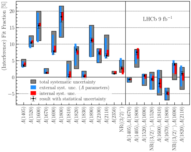
Figure 6: Final results for the fit fractions and interference fit fractions. The vertical line separates the fit from the interference fit fractions. The error bars represent the different sources of uncertainty.

The uncertainties for most observables are dominated by external inputs, specifically the masses and widths of the ${\mathchar 28931\relax}$ states. A future measurement including improved knowledge of the different ${\mathchar 28931\relax}$ baryons and more data will result in a significant reduction of the uncertainties.

The analysis of ${{\mathchar 28931\relax}^{0}_{b}}\!\rightarrow{p}{{K}^{-}}{\gamma}$ decays provides information about the composition of the ${p}{{K}^{-}}$ spectrum with unique access to the heavier ${\mathchar 28931\relax}$ states. A comparison between the composition of the spectrum in ${{\mathchar 28931\relax}^{0}_{b}}\!\rightarrow{p}{{K}^{-}}{\gamma}$ and ${{\mathchar 28931\relax}^{0}_{b}}\!\rightarrow{{J\mskip-3.0mu/\mskip-2.0mu\psi}}{p}{{K}^{-}}$ decays, see Ref. [13], is complicated due to the different phase space and the prominent pentaquark contributions in the latter. Three notable differences are explained in the following. First, the contribution of the sub-threshold resonance ${\mathchar 28931\relax}(1405)$ is much smaller in the radiative mode. Second, the ${\mathchar 28931\relax}(1810)$ state appears small in decays to a photon but large in the ${J\mskip-3.0mu/\mskip-2.0mu\psi}$ case; the neighbouring ${\mathchar 28931\relax}(1820)$ state behaves in the opposite way. This observation reveals a potential ambiguity between the two resonances also echoed in the systematic uncertainties on their fit fractions presented in this paper. Third, the heavy resonances ${\mathchar 28931\relax}(1890)$, ${\mathchar 28931\relax}(2100)$, ${\mathchar 28931\relax}(2110)$, and ${\mathchar 28931\relax}(2350)$ are much larger in the radiative case which is in part due to the phase space enhancement.

In conclusion, an amplitude analysis of the decay ${{\mathchar 28931\relax}^{0}_{b}}\!\rightarrow{p}{{K}^{-}}{\gamma}$ is presented for the first time, based on the helicity formalism. A sample of around 50 000 signal candidates is selected from proton-proton collisions recorded by the LHCb experiment at centre-of-mass energies of 7, 8 and 13 TeV. The default fit model comprises all known $\mathchar 28931\relax$ resonances as well as a nonresonant contribution with quantum numbers $J^{P}=\tfrac{3}{2}^{-}$. The presented amplitude model provides a detailed description of the ${{\mathchar 28931\relax}^{0}_{b}}\!\rightarrow{p}{{K}^{-}}{\gamma}$ decay with possible applications ranging from searches for beyond the Standard Model physics in ${{\mathchar 28931\relax}^{0}_{b}}\!\rightarrow{p}{{K}^{-}}\ell^{+}\ell^{-}$ decays to QCD studies and a possible measurement of the photon polarisation in ${{\mathchar 28931\relax}^{0}_{b}}\!\rightarrow{p}{{K}^{-}}{\gamma}$ decays using polarised ${\mathchar 28931\relax}^{0}_{b}$ baryons from $Z$ decays at future $e^{+}e^{-}$ colliders.

Table 3: Fit fractions (top) and interference fit fractions (bottom) determined using the amplitude model. The values are given in %. The uncertainties from internal and external sources, determined by the numerical convolution procedure are labelled $\sigma_{\text{syst}}^{\text{internal}}$ and $\sigma_{\text{syst}}^{\text{external}}$.

Observable	Value	$\sigma_{\text{stat}}$	$\sigma^{\text{internal}}_{\text{syst}}$	$\sigma^{\text{external}}_{\text{syst}}$	$\sigma_{\text{syst}}$
${\mathchar 28931\relax}(1405)$	3.5	${}_{-0.4}^{+0.3}$	${}_{-0.0}^{+0.9}$	${}_{-0.6}^{+1.3}$	${}_{-0.3}^{+1.9}$
${\mathchar 28931\relax}(1520)$	10.4	${}_{-0.2}^{+0.4}$	${}_{-0.0}^{+0.7}$	${}_{-1.6}^{+1.7}$	${}_{-1.2}^{+2.2}$
${\mathchar 28931\relax}(1600)$	15.6	${}_{-0.9}^{+0.6}$	${}_{-0.2}^{+0.8}$	${}_{-5.0}^{+3.9}$	${}_{-4.6}^{+4.3}$
${\mathchar 28931\relax}(1670)$	1.3	${}_{-0.2}^{+0.2}$	${}_{-0.2}^{+0.3}$	${}_{-0.3}^{+1.2}$	${}_{-0.2}^{+1.3}$
${\mathchar 28931\relax}(1690)$	7.7	${}_{-0.8}^{+0.4}$	${}_{-0.1}^{+1.8}$	${}_{-1.0}^{+5.1}$	${}_{-0.2}^{+6.2}$
${\mathchar 28931\relax}(1800)$	18.3	${}_{-1.6}^{+1.3}$	${}_{-1.1}^{+1.4}$	${}_{-6.0}^{+3.2}$	${}_{-6.2}^{+3.2}$
${\mathchar 28931\relax}(1810)$	0.1	${}_{-0.4}^{+0.9}$	${}_{-0.4}^{+1.7}$	${}_{-0.7}^{+4.0}$	${}_{-0.7}^{+4.8}$
${\mathchar 28931\relax}(1820)$	8.3	${}_{-0.7}^{+0.4}$	${}_{-1.4}^{-0.2}$	${}_{-4.8}^{+1.9}$	${}_{-5.7}^{+1.0}$
${\mathchar 28931\relax}(1830)$	0.3	${}_{-0.4}^{+0.4}$	${}_{-0.5}^{+0.6}$	${}_{-0.9}^{+1.5}$	${}_{-0.9}^{+1.6}$
${\mathchar 28931\relax}(1890)$	11.2	${}_{-0.6}^{+0.7}$	${}_{-0.6}^{+0.5}$	${}_{-5.1}^{+4.3}$	${}_{-4.9}^{+4.6}$
${\mathchar 28931\relax}(2100)$	7.3	${}_{-0.5}^{+0.5}$	${}_{-0.6}^{+1.1}$	${}_{-2.8}^{+1.1}$	${}_{-2.9}^{+1.4}$
${\mathchar 28931\relax}(2110)$	6.5	${}_{-0.7}^{+0.6}$	${}_{-0.0}^{+1.7}$	${}_{-0.9}^{+5.4}$	${}_{-0.2}^{+6.3}$
${\mathchar 28931\relax}(2350)$	1.0	${}_{-0.1}^{+0.2}$	${}_{-0.0}^{+0.8}$	${}_{-0.2}^{+0.0}$	${}_{-0.1}^{+0.8}$
NR$(\nicefrac{{3}}{{2}}^{-})$	2.8	${}_{-0.4}^{+0.5}$	${}_{-1.9}^{+0.2}$	${}_{+0.3}^{+3.0}$	${}_{-1.3}^{+2.4}$
${\mathchar 28931\relax}(1405),{\mathchar 28931\relax}(1670)$	$-0.7$	${}_{-0.2}^{+0.1}$	${}_{-0.2}^{+0.2}$	${}_{-0.8}^{+0.5}$	${}_{-0.9}^{+0.5}$
${\mathchar 28931\relax}(1405),{\mathchar 28931\relax}(1800)$	7.6	${}_{-0.8}^{+0.7}$	${}_{-2.0}^{+1.2}$	${}_{-3.5}^{+0.6}$	${}_{-4.6}^{+0.9}$
${\mathchar 28931\relax}(1520),{\mathchar 28931\relax}(1690)$	0.5	${}_{-0.3}^{+0.5}$	${}_{-0.9}^{+0.3}$	${}_{-2.6}^{+0.6}$	${}_{-3.0}^{+0.5}$
${\mathchar 28931\relax}(1520)$, NR$(\nicefrac{{3}}{{2}}^{-})$	$-0.6$	${}_{-0.4}^{+0.4}$	${}_{-0.6}^{+1.0}$	${}_{-3.2}^{+1.6}$	${}_{-3.0}^{+2.1}$
${\mathchar 28931\relax}(1600),{\mathchar 28931\relax}(1810)$	$-1.9$	${}_{-1.0}^{+1.5}$	${}_{-1.5}^{+1.3}$	${}_{-2.9}^{+4.1}$	${}_{-3.6}^{+3.9}$
${\mathchar 28931\relax}(1670),{\mathchar 28931\relax}(1800)$	$-4.8$	${}_{-0.4}^{+0.5}$	${}_{-0.6}^{+0.4}$	${}_{-2.0}^{+1.5}$	${}_{-2.1}^{+1.5}$
${\mathchar 28931\relax}(1690)$, NR$(\nicefrac{{3}}{{2}}^{-})$	3.9	${}_{-0.4}^{+0.4}$	${}_{-3.0}^{+0.1}$	${}_{-2.7}^{+1.2}$	${}_{-4.7}^{+0.3}$
${\mathchar 28931\relax}(1820),{\mathchar 28931\relax}(2110)$	1.1	${}_{-0.5}^{+0.7}$	${}_{-2.1}^{+0.2}$	${}_{-3.9}^{+2.5}$	${}_{-4.8}^{+1.9}$

Appendices

Appendix A Logarithmic scale plots of $m_{{{\mathchar 28931\relax}^{0}_{b}}}(pK^{-})$

The plots in Fig. 7 are equivalent to the top plots in Fig. 4 with a logarithmic vertical axis in order to make all components visible. This means the plots contain the background corrected data distributions in the proton-kaon invariant mass. The plots also contain the full fit model and the individual components. Note that there are regions where the interference terms become negative but this cannot be displayed on a logarithmic scale.

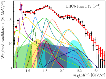
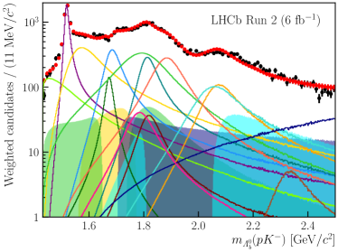
Figure 7: Background-subtracted distribution of the proton-kaon invariant-mass (black dots) for the (left) Run 1 and (right) Run 2 data samples on a logarithmic scale. Also shown is a sample generated according to the result of a simultaneous fit of the default model to the data (red dots) and its components (lines) as well as the contributions due to interference between states with the same quantum numbers $J^{P}$ (shaded areas).

Appendix B Projections for the reduced and second best models

The reduced model consists of the ${\mathchar 28931\relax}$ resonances in Table 1. The best and second best model are based on the reduced model. Contrary to the best model, the second best model has no nonresonant component but instead the mass and width of the ${\mathchar 28931\relax}(2100)$ and ${\mathchar 28931\relax}(2110)$ states are floated in the fit.

Figure 8 shows the fit projections on the proton-photon and kaon-photon invariant-mass, as well as the proton helicity angle for the reduced model. Figure 9 shows the fit projections on the two-body invariant masses and the proton helicity angle for this fit. Figures 10 and 11 show the projections on the proton-kaon invariant mass for the reduced model and the second best model using a logarithmic scale.

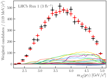
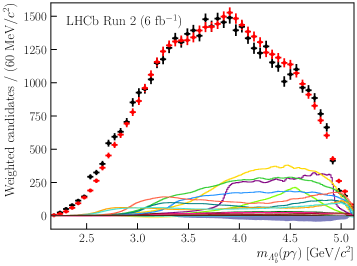
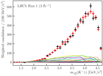
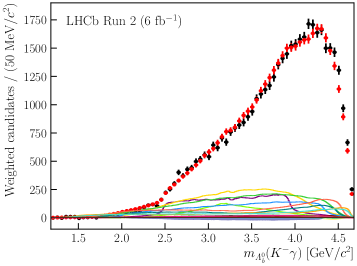
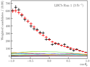
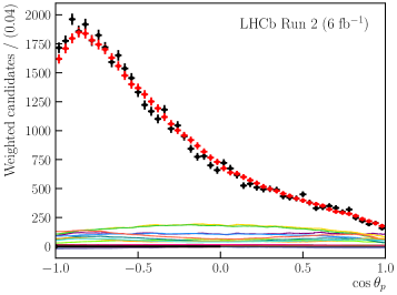
Figure 8: Background-subtracted distribution of (top) the proton-photon invariant-mass, (middle) the kaon-photon invariant-mass, and (bottom) the proton helicity angle (black dots) for the (left) Run 1 and (right) Run 2 data samples. Also shown is a sample generated according to the result of a simultaneous fit of the reduced model to the data (red dots) and its components (lines) as well as the contributions due to interference between states with the same quantum numbers $J^{P}$ (shaded areas). See Fig. 3 for the legend.

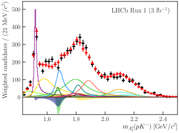
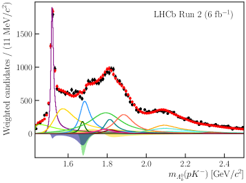
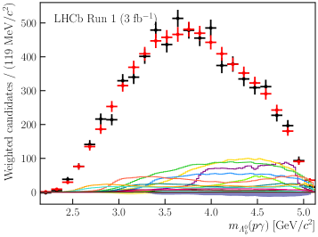
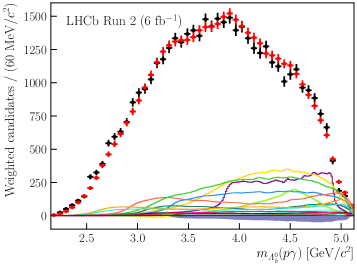
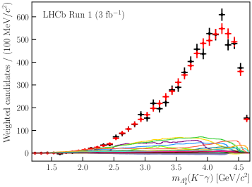
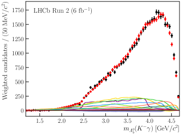
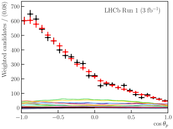
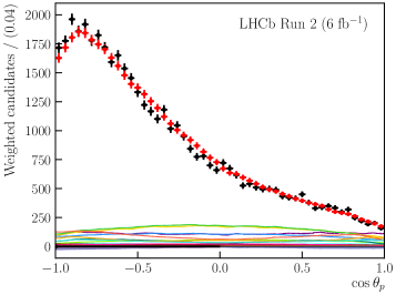
Figure 9: Background-subtracted distribution of (top three rows) the two-body invariant-masses and (bottom row) the proton helicity angle (black dots) for the (left) Run 1 and (right) Run 2 data samples. Also shown is a sample generated according to the result of a simultaneous fit of the second best model to the data (red dots) and its components (lines) as well as the contributions due to interference between states with the same quantum numbers $J^{P}$ (shaded areas). See Fig. 3 for the legend.

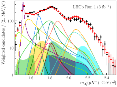
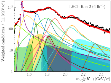
Figure 10: Background-subtracted distribution of the proton-kaon invariant-mass (black dots) for the (left) Run 1 and (right) Run 2 data samples on a logarithmic scale. Also shown is a sample generated according to the result of a simultaneous fit of the reduced model to the data (red dots) and its components (lines) as well as the contributions due to interference between states with the same quantum numbers $J^{P}$ (shaded areas).

Figure 11: Background-subtracted distribution of the proton-kaon invariant-mass (black dots) for the (left) Run 1 and (right) Run 2 data samples on a logarithmic scale. Also shown is a sample generated according to the result of a simultaneous fit of the second best model to the data (red dots) and its components (lines) as well as the contributions due to interference between states with the same quantum numbers $J^{P}$ (shaded areas).

Appendix C Couplings at the best fit point

Tables 4 and 5 give the value of the couplings, $A_{LS}$, obtained from the fit of the default model to data. These values serve primarily to construct the model and cannot be interpreted as measurements. Uncertainties for the couplings are not calculated as they generally are unstable such that minor changes (as are done when estimating systematic uncertainties) can result in very different couplings. The rightmost column indicates which couplings are dependent on the others via Eq. 12.

Table 4: Magnitude, $|A_{LS}|$, and phase, $\arg(A_{LS})$, of the couplings at the best fit point of the default model for resonances ${\mathchar 28931\relax}(1405)$, ${\mathchar 28931\relax}(1520)$, ${\mathchar 28931\relax}(1600)$, ${\mathchar 28931\relax}(1670)$, ${\mathchar 28931\relax}(1690)$, ${\mathchar 28931\relax}(1800)$, ${\mathchar 28931\relax}(1810)$, and ${\mathchar 28931\relax}(1820)$.

Resonance	$2L$	$2S$	$|A_{LS}|$	$\arg(A_{LS})$	additional comment
${\mathchar 28931\relax}(1405)$	0	1	2.890	$-0.672$
	2	1	2.137	$-2.633$
	2	3	1.511	$0.509$	dependent via Eq. 12
	4	3	2.044	$2.470$	dependent via Eq. 12
${\mathchar 28931\relax}(1520)$	0	1	0.400	$-0.016$
	2	1	0.542	$0.147$
	2	3	2.063	$1.649$
	4	3	1.142	$2.083$
	4	5	0.590	$-0.607$	dependent via Eq. 12
	6	5	0.773	$-0.944$	dependent via Eq. 12
${\mathchar 28931\relax}(1600)$	0	1	7.000	$0.970$
	2	1	4.127	$3.057$
	2	3	2.918	$-0.085$	dependent via Eq. 12
	4	3	4.950	$-2.171$	dependent via Eq. 12
${\mathchar 28931\relax}(1670)$	0	1	0.182	$2.694$
	2	1	0.394	$0.549$
	2	3	0.279	$-2.592$	dependent via Eq. 12
	4	3	0.129	$-0.447$	dependent via Eq. 12
${\mathchar 28931\relax}(1690)$	0	1	0.371	$-2.977$
	2	1	2.426	$0.694$
	2	3	1.328	$0.263$
	4	3	2.918	$0.648$
	4	5	1.225	$-2.599$	dependent via Eq. 12
	6	5	1.418	$0.824$	dependent via Eq. 12
${\mathchar 28931\relax}(1800)$	0	1	1.000	$0.000$	fixed in the fit
	2	1	4.418	$-1.498$
	2	3	3.124	$1.643$	dependent via Eq. 12
	4	3	0.707	$3.142$	dependent via Eq. 12
${\mathchar 28931\relax}(1810)$	0	1	1.453	$-2.702$
	2	1	0.374	$-1.129$
	2	3	0.264	$2.012$	dependent via Eq. 12
	4	3	1.027	$0.440$	dependent via Eq. 12
${\mathchar 28931\relax}(1820)$	2	3	0.692	$-2.965$
	4	3	3.166	$-1.937$
	4	5	2.258	$-1.733$
	6	5	3.023	$-1.299$
	6	7	0.931	$2.510$	dependent via Eq. 12
	8	7	2.157	$-1.984$	dependent via Eq. 12

Table 5: Magnitude, $|A_{LS}|$, and phase, $\arg(A_{LS})$, of the couplings at the best fit point of the default model for resonances ${\mathchar 28931\relax}(1830)$, ${\mathchar 28931\relax}(1890)$, ${\mathchar 28931\relax}(2100)$, ${\mathchar 28931\relax}(2110)$, ${\mathchar 28931\relax}(2350)$, and the non-resonant component.

Resonance	$2L$	$2S$	$|A_{LS}|$	$\arg(A_{LS})$	additional comment
${\mathchar 28931\relax}(1830)$	2	3	0.646	$2.337$
	4	3	0.881	$-2.763$
	4	5	0.894	$0.643$
	6	5	0.764	$-2.560$
	6	7	0.536	$2.018$	dependent via Eq. 12
	8	7	0.931	$-2.707$	dependent via Eq. 12
${\mathchar 28931\relax}(1890)$	0	1	2.070	$-1.103$
	2	1	1.312	$0.175$
	2	3	1.449	$3.118$
	4	3	3.918	$1.441$
	4	5	2.724	$-1.376$	dependent via Eq. 12
	6	5	1.455	$0.109$	dependent via Eq. 12
${\mathchar 28931\relax}(2100)$	4	5	2.378	$-0.537$
	6	5	5.087	$1.139$
	6	7	3.192	$1.384$
	8	7	6.932	$1.924$
	8	9	3.088	$-0.778$	dependent via Eq. 12
	10	9	3.946	$1.106$	dependent via Eq. 12
${\mathchar 28931\relax}(2110)$	2	3	2.093	$2.382$
	4	3	6.217	$-2.358$
	4	5	2.348	$-1.664$
	6	5	6.899	$-1.546$
	6	7	3.044	$2.015$	dependent via Eq. 12
	8	7	4.810	$-2.427$	dependent via Eq. 12
${\mathchar 28931\relax}(2350)$	6	7	0.509	$-1.829$
	8	7	0.670	$-0.946$
	8	9	1.751	$-1.344$
	10	9	0.848	$-0.286$
	10	11	0.471	$-2.076$	dependent via Eq. 12
	12	11	0.396	$-0.711$	dependent via Eq. 12
NR$(\nicefrac{{3}}{{2}}^{-})$	0	1	1.368	$0.598$
	2	1	8.811	$3.131$
	2	3	7.525	$-0.006$
	4	3	5.694	$-2.808$
	4	5	2.895	$0.426$	dependent via Eq. 12
	6	5	9.075	$3.132$	dependent via Eq. 12

Appendix D Statistical correlations

Table 6 provides the statistical correlations between the observables.

Table 6: Statistical correlations between the observables in percent obtained from bootstrapping the data. In the interest of space, the $J^{P}$ specification of the nonresonant component of the best model, NR($\tfrac{3}{2}^{-}$), is dropped and the resonances are only referred to by their mass. A single mass refers to the fit fraction of a state, two masses refer to the interference fit fraction of the given combination.

	1405	1520	1600	1670	1690	1800	1810	1820	1830	1890	2100	2110	2350	NR	1405, 1670	1520, 1690	1405, 1800	1670, 1800	1600, 1810	1820, 2110	1520, NR	1690, NR
1405	100
1520	8	100
1600	11	-14	100
1670	-37	-9	-33	100
1690	-7	25	-33	30	100
1800	-24	-13	-8	34	14	100
1810	21	-3	13	-20	-31	-41	100
1820	2	3	2	3	6	-11	3	100
1830	16	20	-8	-20	-27	-36	33	-11	100
1890	-3	4	11	-3	-25	-33	50	1	14	100
2100	-21	-14	-16	21	-24	-0	8	9	28	3	100
2110	-10	20	-5	-9	-2	27	15	-3	-9	23	-26	100
2350	-10	-14	-15	14	4	36	14	-14	-12	-4	-3	19	100
NR	5	7	-9	-6	-36	-2	7	-28	28	3	4	5	9	100
1405, 1670	15	5	47	-52	-7	-19	-5	-6	-5	-8	-31	-20	-21	-23	100
1520, 1690	-2	-11	34	-11	-53	-26	5	2	17	2	22	-28	-18	2	36	100
1405, 1800	-40	-13	-45	18	10	-11	-15	-11	6	-9	26	-8	12	16	-34	2	100
1670, 1800	45	14	26	-93	-27	-58	36	2	26	11	-19	2	-17	2	44	12	-20	100
1600, 1810	-3	-3	-16	5	21	-0	-66	-18	-39	-35	-30	-22	-32	-13	20	-13	-9	-4	100
1820, 2110	22	-18	2	-3	5	-37	-12	-5	11	-34	2	-73	-31	-16	19	20	1	12	31	100
1520, NR	8	-6	-6	1	2	-39	45	-5	9	20	-21	-6	6	-22	-8	-7	-4	16	-12	19	100
1690, NR	-17	-28	-12	17	9	-5	-31	2	-22	-33	2	-54	-3	-8	14	12	13	-14	40	35	-15	100

LHCb collaboration

R. Aaij³⁵ , A.S.W. Abdelmotteleb⁵⁴ , C. Abellan Beteta⁴⁸, F. Abudinén⁵⁴ , T. Ackernley⁵⁸ , B. Adeva⁴⁴ , M. Adinolfi⁵² , P. Adlarson⁷⁸ , C. Agapopoulou⁴⁶ , C.A. Aidala⁷⁹ , Z. Ajaltouni¹¹, S. Akar⁶³ , K. Akiba³⁵ , P. Albicocco²⁵ , J. Albrecht¹⁷ , F. Alessio⁴⁶ , M. Alexander⁵⁷ , A. Alfonso Albero⁴³ , Z. Aliouche⁶⁰ , P. Alvarez Cartelle⁵³ , R. Amalric¹⁵ , S. Amato³ , J.L. Amey⁵² , Y. Amhis^13,46 , L. An⁶ , L. Anderlini²⁴ , M. Andersson⁴⁸ , A. Andreianov⁴¹ , P. Andreola⁴⁸ , M. Andreotti²³ , D. Andreou⁶⁶ , A. Anelli^28,o , D. Ao⁷ , F. Archilli^34,u , M. Argenton²³ , S. Arguedas Cuendis⁹ , A. Artamonov⁴¹ , M. Artuso⁶⁶ , E. Aslanides¹² , M. Atzeni⁶² , B. Audurier¹⁴ , D. Bacher⁶¹ , I. Bachiller Perea¹⁰ , S. Bachmann¹⁹ , M. Bachmayer⁴⁷ , J.J. Back⁵⁴ , P. Baladron Rodriguez⁴⁴ , V. Balagura¹⁴ , W. Baldini²³ , J. Baptista de Souza Leite² , M. Barbetti^24,l , I. R. Barbosa⁶⁷ , R.J. Barlow⁶⁰ , S. Barsuk¹³ , W. Barter⁵⁶ , M. Bartolini⁵³ , J. Bartz⁶⁶ , F. Baryshnikov⁴¹ , J.M. Basels¹⁶ , G. Bassi^32,r , B. Batsukh⁵ , A. Battig¹⁷ , A. Bay⁴⁷ , A. Beck⁵⁴ , M. Becker¹⁷ , F. Bedeschi³² , I.B. Bediaga² , A. Beiter⁶⁶, S. Belin⁴⁴ , V. Bellee⁴⁸ , K. Belous⁴¹ , I. Belov²⁶ , I. Belyaev⁴¹ , G. Benane¹² , G. Bencivenni²⁵ , E. Ben-Haim¹⁵ , A. Berezhnoy⁴¹ , R. Bernet⁴⁸ , S. Bernet Andres⁴² , H.C. Bernstein⁶⁶, C. Bertella⁶⁰ , A. Bertolin³⁰ , C. Betancourt⁴⁸ , F. Betti⁵⁶ , J.  Bex⁵³ , Ia. Bezshyiko⁴⁸ , J. Bhom³⁸ , M.S. Bieker¹⁷ , N.V. Biesuz²³ , P. Billoir¹⁵ , A. Biolchini³⁵ , M. Birch⁵⁹ , F.C.R. Bishop¹⁰ , A. Bitadze⁶⁰ , A. Bizzeti , M.P. Blago⁵³ , T. Blake⁵⁴ , F. Blanc⁴⁷ , J.E. Blank¹⁷ , S. Blusk⁶⁶ , D. Bobulska⁵⁷ , V. Bocharnikov⁴¹ , J.A. Boelhauve¹⁷ , O. Boente Garcia¹⁴ , T. Boettcher⁶³ , A.  Bohare⁵⁶ , A. Boldyrev⁴¹ , C.S. Bolognani⁷⁶ , R. Bolzonella^23,k , N. Bondar⁴¹ , F. Borgato^30,46 , S. Borghi⁶⁰ , M. Borsato^28,o , J.T. Borsuk³⁸ , S.A. Bouchiba⁴⁷ , T.J.V. Bowcock⁵⁸ , A. Boyer⁴⁶ , C. Bozzi²³ , M.J. Bradley⁵⁹, S. Braun⁶⁴ , A. Brea Rodriguez⁴⁴ , N. Breer¹⁷ , J. Brodzicka³⁸ , A. Brossa Gonzalo⁴⁴ , J. Brown⁵⁸ , D. Brundu²⁹ , A. Buonaura⁴⁸ , L. Buonincontri³⁰ , A.T. Burke⁶⁰ , C. Burr⁴⁶ , A. Bursche⁶⁹, A. Butkevich⁴¹ , J.S. Butter⁵³ , J. Buytaert⁴⁶ , W. Byczynski⁴⁶ , S. Cadeddu²⁹ , H. Cai⁷¹, R. Calabrese^23,k , L. Calefice¹⁷ , S. Cali²⁵ , M. Calvi^28,o , M. Calvo Gomez⁴² , J. Cambon Bouzas⁴⁴ , P. Campana²⁵ , D.H. Campora Perez⁷⁶ , A.F. Campoverde Quezada⁷ , S. Capelli^28,o , L. Capriotti²³ , R. Caravaca-Mora⁹ , A. Carbone^22,i , L. Carcedo Salgado⁴⁴ , R. Cardinale^26,m , A. Cardini²⁹ , P. Carniti^28,o , L. Carus¹⁹, A. Casais Vidal⁶² , R. Caspary¹⁹ , G. Casse⁵⁸ , J. Castro Godinez⁹ , M. Cattaneo⁴⁶ , G. Cavallero²³ , V. Cavallini^23,k , S. Celani⁴⁷ , J. Cerasoli¹² , D. Cervenkov⁶¹ , S.  Cesare^27,n , A.J. Chadwick⁵⁸ , I. Chahrour⁷⁹ , M. Charles¹⁵ , Ph. Charpentier⁴⁶ , C.A. Chavez Barajas⁵⁸ , M. Chefdeville¹⁰ , C. Chen¹² , S. Chen⁵ , Z. Chen⁷ , A. Chernov³⁸ , S. Chernyshenko⁵⁰ , V. Chobanova^44,y , S. Cholak⁴⁷ , M. Chrzaszcz³⁸ , A. Chubykin⁴¹ , V. Chulikov⁴¹ , P. Ciambrone²⁵ , M.F. Cicala⁵⁴ , X. Cid Vidal⁴⁴ , G. Ciezarek⁴⁶ , P. Cifra⁴⁶ , P.E.L. Clarke⁵⁶ , M. Clemencic⁴⁶ , H.V. Cliff⁵³ , J. Closier⁴⁶ , J.L. Cobbledick⁶⁰ , C. Cocha Toapaxi¹⁹ , V. Coco⁴⁶ , J. Cogan¹² , E. Cogneras¹¹ , L. Cojocariu⁴⁰ , P. Collins⁴⁶ , T. Colombo⁴⁶ , A. Comerma-Montells⁴³ , L. Congedo²¹ , A. Contu²⁹ , N. Cooke⁵⁷ , I. Corredoira ⁴⁴ , A. Correia¹⁵ , G. Corti⁴⁶ , J.J. Cottee Meldrum⁵², B. Couturier⁴⁶ , D.C. Craik⁴⁸ , M. Cruz Torres^2,g , E. Curras Rivera⁴⁷ , R. Currie⁵⁶ , C.L. Da Silva⁶⁵ , S. Dadabaev⁴¹ , L. Dai⁶⁸ , X. Dai⁶ , E. Dall’Occo¹⁷ , J. Dalseno⁴⁴ , C. D’Ambrosio⁴⁶ , J. Daniel¹¹ , A. Danilina⁴¹ , P. d’Argent²¹ , A.  Davidson⁵⁴ , J.E. Davies⁶⁰ , A. Davis⁶⁰ , O. De Aguiar Francisco⁶⁰ , C. De Angelis^29,j , J. de Boer³⁵ , K. De Bruyn⁷⁵ , S. De Capua⁶⁰ , M. De Cian^19,46 , U. De Freitas Carneiro Da Graca^2,b , E. De Lucia²⁵ , J.M. De Miranda² , L. De Paula³ , M. De Serio^21,h , D. De Simone⁴⁸ , P. De Simone²⁵ , F. De Vellis¹⁷ , J.A. de Vries⁷⁶ , F. Debernardis^21,h , D. Decamp¹⁰ , V. Dedu¹² , L. Del Buono¹⁵ , B. Delaney⁶² , H.-P. Dembinski¹⁷ , J. Deng⁸ , V. Denysenko⁴⁸ , O. Deschamps¹¹ , F. Dettori^29,j , B. Dey⁷⁴ , P. Di Nezza²⁵ , I. Diachkov⁴¹ , S. Didenko⁴¹ , S. Ding⁶⁶ , V. Dobishuk⁵⁰ , A. D.  Docheva⁵⁷ , A. Dolmatov⁴¹, C. Dong⁴ , A.M. Donohoe²⁰ , F. Dordei²⁹ , A.C. dos Reis² , L. Douglas⁵⁷, A.G. Downes¹⁰ , W. Duan⁶⁹ , P. Duda⁷⁷ , M.W. Dudek³⁸ , L. Dufour⁴⁶ , V. Duk³¹ , P. Durante⁴⁶ , M. M. Duras⁷⁷ , J.M. Durham⁶⁵ , A. Dziurda³⁸ , A. Dzyuba⁴¹ , S. Easo^55,46 , E. Eckstein⁷³, U. Egede¹ , A. Egorychev⁴¹ , V. Egorychev⁴¹ , C. Eirea Orro⁴⁴, S. Eisenhardt⁵⁶ , E. Ejopu⁶⁰ , S. Ek-In⁴⁷ , L. Eklund⁷⁸ , M. Elashri⁶³ , J. Ellbracht¹⁷ , S. Ely⁵⁹ , A. Ene⁴⁰ , E. Epple⁶³ , S. Escher¹⁶ , J. Eschle⁴⁸ , S. Esen⁴⁸ , T. Evans⁶⁰ , F. Fabiano^29,j,46 , L.N. Falcao² , Y. Fan⁷ , B. Fang^71,13 , L. Fantini^31,q , M. Faria⁴⁷ , K.  Farmer⁵⁶ , D. Fazzini^28,o , L. Felkowski⁷⁷ , M. Feng^5,7 , M. Feo⁴⁶ , M. Fernandez Gomez⁴⁴ , A.D. Fernez⁶⁴ , F. Ferrari²² , F. Ferreira Rodrigues³ , S. Ferreres Sole³⁵ , M. Ferrillo⁴⁸ , M. Ferro-Luzzi⁴⁶ , S. Filippov⁴¹ , R.A. Fini²¹ , M. Fiorini^23,k , M. Firlej³⁷ , K.M. Fischer⁶¹ , D.S. Fitzgerald⁷⁹ , C. Fitzpatrick⁶⁰ , T. Fiutowski³⁷ , F. Fleuret¹⁴ , M. Fontana²² , F. Fontanelli^26,m , L. F.  Foreman⁶⁰ , R. Forty⁴⁶ , D. Foulds-Holt⁵³ , M. Franco Sevilla⁶⁴ , M. Frank⁴⁶ , E. Franzoso^23,k , G. Frau¹⁹ , C. Frei⁴⁶ , D.A. Friday⁶⁰ , L. Frontini^27,n , J. Fu⁷ , Q. Fuehring¹⁷ , Y. Fujii¹ , T. Fulghesu¹⁵ , E. Gabriel³⁵ , G. Galati^21,h , M.D. Galati³⁵ , A. Gallas Torreira⁴⁴ , D. Galli^22,i , S. Gambetta⁵⁶ , M. Gandelman³ , P. Gandini²⁷ , H. Gao⁷ , R. Gao⁶¹ , Y. Gao⁸ , Y. Gao⁶ , Y. Gao⁸, M. Garau^29,j , L.M. Garcia Martin⁴⁷ , P. Garcia Moreno⁴³ , J. García Pardiñas⁴⁶ , B. Garcia Plana⁴⁴, K. G.  Garg⁸ , L. Garrido⁴³ , C. Gaspar⁴⁶ , R.E. Geertsema³⁵ , L.L. Gerken¹⁷ , E. Gersabeck⁶⁰ , M. Gersabeck⁶⁰ , T. Gershon⁵⁴ , Z. Ghorbanimoghaddam⁵², L. Giambastiani³⁰ , F. I. Giasemis^15,e , V. Gibson⁵³ , H.K. Giemza³⁹ , A.L. Gilman⁶¹ , M. Giovannetti²⁵ , A. Gioventù⁴³ , P. Gironella Gironell⁴³ , C. Giugliano^23,k , M.A. Giza³⁸ , E.L. Gkougkousis⁵⁹ , F.C. Glaser^13,19 , V.V. Gligorov¹⁵ , C. Göbel⁶⁷ , E. Golobardes⁴² , D. Golubkov⁴¹ , A. Golutvin^59,41,46 , A. Gomes^2,a,† , S. Gomez Fernandez⁴³ , F. Goncalves Abrantes⁶¹ , M. Goncerz³⁸ , G. Gong⁴ , J. A. Gooding¹⁷ , I.V. Gorelov⁴¹ , C. Gotti²⁸ , J.P. Grabowski⁷³ , L.A. Granado Cardoso⁴⁶ , E. Graugés⁴³ , E. Graverini^47,s , L. Grazette⁵⁴ , G. Graziani , A. T. Grecu⁴⁰ , L.M. Greeven³⁵ , N.A. Grieser⁶³ , L. Grillo⁵⁷ , S. Gromov⁴¹ , C.  Gu¹⁴ , M. Guarise²³ , M. Guittiere¹³ , V. Guliaeva⁴¹ , P. A. Günther¹⁹ , A.-K. Guseinov⁴¹ , E. Gushchin⁴¹ , Y. Guz^6,41,46 , T. Gys⁴⁶ , T. Hadavizadeh¹ , C. Hadjivasiliou⁶⁴ , G. Haefeli⁴⁷ , C. Haen⁴⁶ , J. Haimberger⁴⁶ , M. Hajheidari⁴⁶, T. Halewood-leagas⁵⁸ , M.M. Halvorsen⁴⁶ , P.M. Hamilton⁶⁴ , J. Hammerich⁵⁸ , Q. Han⁸ , X. Han¹⁹ , S. Hansmann-Menzemer¹⁹ , L. Hao⁷ , N. Harnew⁶¹ , T. Harrison⁵⁸ , M. Hartmann¹³ , C. Hasse⁴⁶ , J. He^7,c , K. Heijhoff³⁵ , F. Hemmer⁴⁶ , C. Henderson⁶³ , R.D.L. Henderson^1,54 , A.M. Hennequin⁴⁶ , K. Hennessy⁵⁸ , L. Henry⁴⁷ , J. Herd⁵⁹ , P. Herrero Gascon¹⁹ , J. Heuel¹⁶ , A. Hicheur³ , G. Hijano Mendizabal⁴⁸, D. Hill⁴⁷ , S.E. Hollitt¹⁷ , J. Horswill⁶⁰ , R. Hou⁸ , Y. Hou¹⁰ , N. Howarth⁵⁸, J. Hu¹⁹, J. Hu⁶⁹ , W. Hu⁶ , X. Hu⁴ , W. Huang⁷ , W. Hulsbergen³⁵ , R.J. Hunter⁵⁴ , M. Hushchyn⁴¹ , D. Hutchcroft⁵⁸ , M. Idzik³⁷ , D. Ilin⁴¹ , P. Ilten⁶³ , A. Inglessi⁴¹ , A. Iniukhin⁴¹ , A. Ishteev⁴¹ , K. Ivshin⁴¹ , R. Jacobsson⁴⁶ , H. Jage¹⁶ , S.J. Jaimes Elles^45,72 , S. Jakobsen⁴⁶ , E. Jans³⁵ , B.K. Jashal⁴⁵ , A. Jawahery^64,46 , V. Jevtic¹⁷ , E. Jiang⁶⁴ , X. Jiang^5,7 , Y. Jiang⁷ , Y. J.  Jiang⁶ , M. John⁶¹ , D. Johnson⁵¹ , C.R. Jones⁵³ , T.P. Jones⁵⁴ , S. Joshi³⁹ , B. Jost⁴⁶ , N. Jurik⁴⁶ , I. Juszczak³⁸ , D. Kaminaris⁴⁷ , S. Kandybei⁴⁹ , Y. Kang⁴ , M. Karacson⁴⁶ , D. Karpenkov⁴¹ , M. Karpov⁴¹ , A. M.  Kauniskangas⁴⁷ , J.W. Kautz⁶³ , F. Keizer⁴⁶ , D.M. Keller⁶⁶ , M. Kenzie⁵³ , T. Ketel³⁵ , B. Khanji⁶⁶ , A. Kharisova⁴¹ , S. Kholodenko³² , G. Khreich¹³ , T. Kirn¹⁶ , V.S. Kirsebom⁴⁷ , O. Kitouni⁶² , S. Klaver³⁶ , N. Kleijne^32,r , K. Klimaszewski³⁹ , M.R. Kmiec³⁹ , S. Koliiev⁵⁰ , L. Kolk¹⁷ , A. Konoplyannikov⁴¹ , P. Kopciewicz^37,46 , P. Koppenburg³⁵ , M. Korolev⁴¹ , I. Kostiuk³⁵ , O. Kot⁵⁰, S. Kotriakhova , A. Kozachuk⁴¹ , P. Kravchenko⁴¹ , L. Kravchuk⁴¹ , M. Kreps⁵⁴ , S. Kretzschmar¹⁶ , P. Krokovny⁴¹ , W. Krupa⁶⁶ , W. Krzemien³⁹ , J. Kubat¹⁹, S. Kubis⁷⁷ , W. Kucewicz³⁸ , M. Kucharczyk³⁸ , V. Kudryavtsev⁴¹ , E. Kulikova⁴¹ , A. Kupsc⁷⁸ , B. K.  Kutsenko¹² , D. Lacarrere⁴⁶ , A. Lai²⁹ , A. Lampis²⁹ , D. Lancierini⁴⁸ , C. Landesa Gomez⁴⁴ , J.J. Lane¹ , R. Lane⁵² , C. Langenbruch¹⁹ , J. Langer¹⁷ , O. Lantwin⁴¹ , T. Latham⁵⁴ , F. Lazzari^32,s , C. Lazzeroni⁵¹ , R. Le Gac¹² , S.H. Lee⁷⁹ , R. Lefèvre¹¹ , A. Leflat⁴¹ , S. Legotin⁴¹ , M. Lehuraux⁵⁴ , O. Leroy¹² , T. Lesiak³⁸ , B. Leverington¹⁹ , A. Li⁴ , H. Li⁶⁹ , K. Li⁸ , L. Li⁶⁰ , P. Li⁴⁶ , P.-R. Li⁷⁰ , S. Li⁸ , T. Li^5,d , T. Li⁶⁹ , Y. Li⁸, Y. Li⁵ , Z. Li⁶⁶ , Z. Lian⁴ , X. Liang⁶⁶ , C. Lin⁷ , T. Lin⁵⁵ , R. Lindner⁴⁶ , V. Lisovskyi⁴⁷ , R. Litvinov^29,j , F. L.  Liu¹ , G. Liu⁶⁹ , H. Liu⁷ , K. Liu⁷⁰ , Q. Liu⁷ , S. Liu^5,7 , Y. Liu⁵⁶ , Y. Liu⁷⁰, Y. L.  Liu⁵⁹ , A. Lobo Salvia⁴³ , A. Loi²⁹ , J. Lomba Castro⁴⁴ , T. Long⁵³ , J.H. Lopes³ , A. Lopez Huertas⁴³ , S. López Soliño⁴⁴ , G.H. Lovell⁵³ , C. Lucarelli^24,l , D. Lucchesi^30,p , S. Luchuk⁴¹ , M. Lucio Martinez⁷⁶ , V. Lukashenko^35,50 , Y. Luo⁶ , A. Lupato³⁰ , E. Luppi^23,k , K. Lynch²⁰ , X.-R. Lyu⁷ , G. M.  Ma⁴ , R. Ma⁷ , S. Maccolini¹⁷ , F. Machefert¹³ , F. Maciuc⁴⁰ , B. M.  Mack⁶⁶ , I. Mackay⁶¹ , L. M.  Mackey⁶⁶ , L.R. Madhan Mohan⁵³ , M. M.  Madurai⁵¹ , A. Maevskiy⁴¹ , D. Magdalinski³⁵ , D. Maisuzenko⁴¹ , M.W. Majewski³⁷, J.J. Malczewski³⁸ , S. Malde⁶¹ , B. Malecki^38,46 , L. Malentacca⁴⁶, A. Malinin⁴¹ , T. Maltsev⁴¹ , G. Manca^29,j , G. Mancinelli¹² , C. Mancuso^27,13,n , R. Manera Escalero⁴³, D. Manuzzi²² , D. Marangotto^27,n , J.F. Marchand¹⁰ , R. Marchevski⁴⁷ , U. Marconi²² , S. Mariani⁴⁶ , C. Marin Benito⁴³ , J. Marks¹⁹ , A.M. Marshall⁵² , P.J. Marshall⁵⁸, G. Martelli^31,q , G. Martellotti³³ , L. Martinazzoli⁴⁶ , M. Martinelli^28,o , D. Martinez Santos⁴⁴ , F. Martinez Vidal⁴⁵ , A. Massafferri² , M. Materok¹⁶ , R. Matev⁴⁶ , A. Mathad⁴⁸ , V. Matiunin⁴¹ , C. Matteuzzi⁶⁶ , K.R. Mattioli¹⁴ , A. Mauri⁵⁹ , E. Maurice¹⁴ , J. Mauricio⁴³ , P. Mayencourt⁴⁷ , M. Mazurek⁴⁶ , M. McCann⁵⁹ , L. Mcconnell²⁰ , T.H. McGrath⁶⁰ , N.T. McHugh⁵⁷ , A. McNab⁶⁰ , R. McNulty²⁰ , B. Meadows⁶³ , G. Meier¹⁷ , D. Melnychuk³⁹ , M. Merk^35,76 , A. Merli^27,n , L. Meyer Garcia³ , D. Miao^5,7 , H. Miao⁷ , M. Mikhasenko^73,f , D.A. Milanes⁷² , A. Minotti^28,o , E. Minucci⁶⁶ , T. Miralles¹¹ , S.E. Mitchell⁵⁶ , B. Mitreska¹⁷ , D.S. Mitzel¹⁷ , A. Modak⁵⁵ , A. Mödden ¹⁷ , R.A. Mohammed⁶¹ , R.D. Moise¹⁶ , S. Mokhnenko⁴¹ , T. Mombächer⁴⁶ , M. Monk^54,1 , I.A. Monroy⁷² , S. Monteil¹¹ , A. Morcillo Gomez⁴⁴ , G. Morello²⁵ , M.J. Morello^32,r , M.P. Morgenthaler¹⁹ , J. Moron³⁷ , A.B. Morris⁴⁶ , A.G. Morris¹² , R. Mountain⁶⁶ , H. Mu⁴ , Z. M.  Mu⁶ , E. Muhammad⁵⁴ , F. Muheim⁵⁶ , M. Mulder⁷⁵ , K. Müller⁴⁸ , F. Mũnoz-Rojas⁹ , R. Murta⁵⁹ , P. Naik⁵⁸ , T. Nakada⁴⁷ , R. Nandakumar⁵⁵ , T. Nanut⁴⁶ , I. Nasteva³ , M. Needham⁵⁶ , N. Neri^27,n , S. Neubert⁷³ , N. Neufeld⁴⁶ , P. Neustroev⁴¹, R. Newcombe⁵⁹, J. Nicolini^17,13 , D. Nicotra⁷⁶ , E.M. Niel⁴⁷ , N. Nikitin⁴¹ , P. Nogga⁷³, N.S. Nolte⁶² , C. Normand^10,29 , J. Novoa Fernandez⁴⁴ , G. Nowak⁶³ , C. Nunez⁷⁹ , H. N.  Nur⁵⁷ , A. Oblakowska-Mucha³⁷ , V. Obraztsov⁴¹ , T. Oeser¹⁶ , S. Okamura^23,k,46 , R. Oldeman^29,j , F. Oliva⁵⁶ , M. Olocco¹⁷ , C.J.G. Onderwater⁷⁶ , R.H. O’Neil⁵⁶ , J.M. Otalora Goicochea³ , T. Ovsiannikova⁴¹ , P. Owen⁴⁸ , A. Oyanguren⁴⁵ , O. Ozcelik⁵⁶ , K.O. Padeken⁷³ , B. Pagare⁵⁴ , P.R. Pais¹⁹ , T. Pajero⁶¹ , A. Palano²¹ , M. Palutan²⁵ , G. Panshin⁴¹ , L. Paolucci⁵⁴ , A. Papanestis⁵⁵ , M. Pappagallo^21,h , L.L. Pappalardo^23,k , C. Pappenheimer⁶³ , C. Parkes⁶⁰ , B. Passalacqua^23,k , G. Passaleva²⁴ , D. Passaro^32,r , A. Pastore²¹ , M. Patel⁵⁹ , J. Patoc⁶¹ , C. Patrignani^22,i , C.J. Pawley⁷⁶ , A. Pellegrino³⁵ , M. Pepe Altarelli²⁵ , S. Perazzini²² , D. Pereima⁴¹ , A. Pereiro Castro⁴⁴ , P. Perret¹¹ , A. Perro⁴⁶ , K. Petridis⁵² , A. Petrolini^26,m , S. Petrucci⁵⁶ , J. P.  Pfaller⁶³ , H. Pham⁶⁶ , L. Pica^32,r , M. Piccini³¹ , B. Pietrzyk¹⁰ , G. Pietrzyk¹³ , D. Pinci³³ , F. Pisani⁴⁶ , M. Pizzichemi^28,o , V. Placinta⁴⁰ , M. Plo Casasus⁴⁴ , F. Polci^15,46 , M. Poli Lener²⁵ , A. Poluektov¹² , N. Polukhina⁴¹ , I. Polyakov⁴⁶ , E. Polycarpo³ , S. Ponce⁴⁶ , D. Popov⁷ , S. Poslavskii⁴¹ , K. Prasanth³⁸ , C. Prouve⁴⁴ , V. Pugatch⁵⁰ , G. Punzi^32,s , W. Qian⁷ , N. Qin⁴ , S. Qu⁴ , R. Quagliani⁴⁷ , R.I. Rabadan Trejo⁵⁴ , B. Rachwal³⁷ , J.H. Rademacker⁵² , M. Rama³² , M.  Ramírez García⁷⁹ , M. Ramos Pernas⁵⁴ , M.S. Rangel³ , F. Ratnikov⁴¹ , G. Raven³⁶ , M. Rebollo De Miguel⁴⁵ , F. Redi⁴⁶ , J. Reich⁵² , F. Reiss⁶⁰ , Z. Ren⁷ , P.K. Resmi⁶¹ , R. Ribatti^32,r , G. R.  Ricart^14,80 , D. Riccardi^32,r , S. Ricciardi⁵⁵ , K. Richardson⁶² , M. Richardson-Slipper⁵⁶ , K. Rinnert⁵⁸ , P. Robbe¹³ , G. Robertson⁵⁷ , E. Rodrigues^58,46 , E. Rodriguez Fernandez⁴⁴ , J.A. Rodriguez Lopez⁷² , E. Rodriguez Rodriguez⁴⁴ , A. Rogovskiy⁵⁵ , D.L. Rolf⁴⁶ , A. Rollings⁶¹ , P. Roloff⁴⁶ , V. Romanovskiy⁴¹ , M. Romero Lamas⁴⁴ , A. Romero Vidal⁴⁴ , G. Romolini²³ , F. Ronchetti⁴⁷ , M. Rotondo²⁵ , S. R.  Roy¹⁹ , M.S. Rudolph⁶⁶ , T. Ruf⁴⁶ , M. Ruiz Diaz¹⁹ , R.A. Ruiz Fernandez⁴⁴ , J. Ruiz Vidal^78,z , A. Ryzhikov⁴¹ , J. Ryzka³⁷ , J.J. Saborido Silva⁴⁴ , R. Sadek¹⁴ , N. Sagidova⁴¹ , N. Sahoo⁵¹ , B. Saitta^29,j , M. Salomoni^28,o , C. Sanchez Gras³⁵ , I. Sanderswood⁴⁵ , R. Santacesaria³³ , C. Santamarina Rios⁴⁴ , M. Santimaria²⁵ , L. Santoro ² , E. Santovetti³⁴ , A. Saputi^23,46 , D. Saranin⁴¹ , G. Sarpis⁵⁶ , M. Sarpis⁷³ , A. Sarti³³ , C. Satriano^33,t , A. Satta³⁴ , M. Saur⁶ , D. Savrina⁴¹ , H. Sazak¹¹ , L.G. Scantlebury Smead⁶¹ , A. Scarabotto¹⁵ , S. Schael¹⁶ , S. Scherl⁵⁸ , A. M.  Schertz⁷⁴ , M. Schiller⁵⁷ , H. Schindler⁴⁶ , M. Schmelling¹⁸ , B. Schmidt⁴⁶ , S. Schmitt¹⁶ , H. Schmitz⁷³, O. Schneider⁴⁷ , A. Schopper⁴⁶ , N. Schulte¹⁷ , S. Schulte⁴⁷ , M.H. Schune¹³ , R. Schwemmer⁴⁶ , G. Schwering¹⁶ , B. Sciascia²⁵ , A. Sciuccati⁴⁶ , S. Sellam⁴⁴ , A. Semennikov⁴¹ , M. Senghi Soares³⁶ , A. Sergi^26,m , N. Serra^48,46 , L. Sestini³⁰ , A. Seuthe¹⁷ , Y. Shang⁶ , D.M. Shangase⁷⁹ , M. Shapkin⁴¹ , R. S.  Sharma⁶⁶ , I. Shchemerov⁴¹ , L. Shchutska⁴⁷ , T. Shears⁵⁸ , L. Shekhtman⁴¹ , Z. Shen⁶ , S. Sheng^5,7 , V. Shevchenko⁴¹ , B. Shi⁷ , E.B. Shields^28,o , Y. Shimizu¹³ , E. Shmanin⁴¹ , R. Shorkin⁴¹ , J.D. Shupperd⁶⁶ , R. Silva Coutinho⁶⁶ , G. Simi³⁰ , S. Simone^21,h , N. Skidmore⁶⁰ , R. Skuza¹⁹ , T. Skwarnicki⁶⁶ , M.W. Slater⁵¹ , J.C. Smallwood⁶¹ , E. Smith⁶² , K. Smith⁶⁵ , M. Smith⁵⁹ , A. Snoch³⁵ , L. Soares Lavra⁵⁶ , M.D. Sokoloff⁶³ , F.J.P. Soler⁵⁷ , A. Solomin^41,52 , A. Solovev⁴¹ , I. Solovyev⁴¹ , R. Song¹ , Y. Song⁴⁷ , Y. Song⁴ , Y. S.  Song⁶ , F.L. Souza De Almeida⁶⁶ , B. Souza De Paula³ , E. Spadaro Norella^27,n , E. Spedicato²² , J.G. Speer¹⁷ , E. Spiridenkov⁴¹, P. Spradlin⁵⁷ , V. Sriskaran⁴⁶ , F. Stagni⁴⁶ , M. Stahl⁴⁶ , S. Stahl⁴⁶ , S. Stanislaus⁶¹ , E.N. Stein⁴⁶ , O. Steinkamp⁴⁸ , O. Stenyakin⁴¹, H. Stevens¹⁷ , D. Strekalina⁴¹ , Y. Su⁷ , F. Suljik⁶¹ , J. Sun²⁹ , L. Sun⁷¹ , Y. Sun⁶⁴ , P.N. Swallow⁵¹ , K. Swientek³⁷ , F. Swystun⁵⁴ , A. Szabelski³⁹ , T. Szumlak³⁷ , M. Szymanski⁴⁶ , Y. Tan⁴ , S. Taneja⁶⁰ , M.D. Tat⁶¹ , A. Terentev⁴⁸ , F. Terzuoli^32,v , F. Teubert⁴⁶ , E. Thomas⁴⁶ , D.J.D. Thompson⁵¹ , H. Tilquin⁵⁹ , V. Tisserand¹¹ , S. T’Jampens¹⁰ , M. Tobin⁵ , L. Tomassetti^23,k , G. Tonani^27,n,46 , X. Tong⁶ , D. Torres Machado² , L. Toscano¹⁷ , D.Y. Tou⁴ , C. Trippl⁴² , G. Tuci¹⁹ , N. Tuning³⁵ , L.H. Uecker¹⁹ , A. Ukleja³⁷ , D.J. Unverzagt¹⁹ , E. Ursov⁴¹ , A. Usachov³⁶ , A. Ustyuzhanin⁴¹ , U. Uwer¹⁹ , V. Vagnoni²² , A. Valassi⁴⁶ , G. Valenti²² , N. Valls Canudas⁴² , H. Van Hecke⁶⁵ , E. van Herwijnen⁵⁹ , C.B. Van Hulse^44,x , R. Van Laak⁴⁷ , M. van Veghel³⁵ , R. Vazquez Gomez⁴³ , P. Vazquez Regueiro⁴⁴ , C. Vázquez Sierra⁴⁴ , S. Vecchi²³ , J.J. Velthuis⁵² , M. Veltri^24,w , A. Venkateswaran⁴⁷ , M. Vesterinen⁵⁴ , M. Vieites Diaz⁴⁶ , X. Vilasis-Cardona⁴² , E. Vilella Figueras⁵⁸ , A. Villa²² , P. Vincent¹⁵ , F.C. Volle¹³ , D. vom Bruch¹² , V. Vorobyev⁴¹, N. Voropaev⁴¹ , K. Vos⁷⁶ , G. Vouters¹⁰, C. Vrahas⁵⁶ , J. Walsh³² , E.J. Walton¹ , G. Wan⁶ , C. Wang¹⁹ , G. Wang⁸ , J. Wang⁶ , J. Wang⁵ , J. Wang⁴ , J. Wang⁷¹ , M. Wang²⁷ , N. W.  Wang⁷ , R. Wang⁵² , X. Wang⁶⁹ , X. W.  Wang⁵⁹ , Y. Wang⁸ , Z. Wang¹³ , Z. Wang⁴ , Z. Wang⁷ , J.A. Ward^54,1 , M. Waterlaat⁴⁶, N.K. Watson⁵¹ , D. Websdale⁵⁹ , Y. Wei⁶ , B.D.C. Westhenry⁵² , D.J. White⁶⁰ , M. Whitehead⁵⁷ , A.R. Wiederhold⁵⁴ , D. Wiedner¹⁷ , G. Wilkinson⁶¹ , M.K. Wilkinson⁶³ , M. Williams⁶² , M.R.J. Williams⁵⁶ , R. Williams⁵³ , F.F. Wilson⁵⁵ , W. Wislicki³⁹ , M. Witek³⁸ , L. Witola¹⁹ , C.P. Wong⁶⁵ , G. Wormser¹³ , S.A. Wotton⁵³ , H. Wu⁶⁶ , J. Wu⁸ , Y. Wu⁶ , K. Wyllie⁴⁶ , S. Xian⁶⁹, Z. Xiang⁵ , Y. Xie⁸ , A. Xu³² , J. Xu⁷ , L. Xu⁴ , L. Xu⁴ , M. Xu⁵⁴ , Z. Xu¹¹ , Z. Xu⁷ , Z. Xu⁵ , D. Yang⁴ , S. Yang⁷ , X. Yang⁶ , Y. Yang^26,m , Z. Yang⁶ , Z. Yang⁶⁴ , V. Yeroshenko¹³ , H. Yeung⁶⁰ , H. Yin⁸ , C. Y.  Yu⁶ , J. Yu⁶⁸ , X. Yuan⁵ , E. Zaffaroni⁴⁷ , M. Zavertyaev¹⁸ , M. Zdybal³⁸ , M. Zeng⁴ , C. Zhang⁶ , D. Zhang⁸ , J. Zhang⁷ , L. Zhang⁴ , S. Zhang⁶⁸ , S. Zhang⁶ , Y. Zhang⁶ , Y. Z.  Zhang⁴ , Y. Zhao¹⁹ , A. Zharkova⁴¹ , A. Zhelezov¹⁹ , X. Z.  Zheng⁴ , Y. Zheng⁷ , T. Zhou⁶ , X. Zhou⁸ , Y. Zhou⁷ , V. Zhovkovska⁵⁴ , L. Z.  Zhu⁷ , X. Zhu⁴ , X. Zhu⁸ , Z. Zhu⁷ , V. Zhukov^16,41 , J. Zhuo⁴⁵ , Q. Zou^5,7 , D. Zuliani³⁰ , G. Zunica⁶⁰ .

¹School of Physics and Astronomy, Monash University, Melbourne, Australia
²Centro Brasileiro de Pesquisas Físicas (CBPF), Rio de Janeiro, Brazil
³Universidade Federal do Rio de Janeiro (UFRJ), Rio de Janeiro, Brazil
⁴Center for High Energy Physics, Tsinghua University, Beijing, China
⁵Institute Of High Energy Physics (IHEP), Beijing, China
⁶School of Physics State Key Laboratory of Nuclear Physics and Technology, Peking University, Beijing, China
⁷University of Chinese Academy of Sciences, Beijing, China
⁸Institute of Particle Physics, Central China Normal University, Wuhan, Hubei, China
⁹Consejo Nacional de Rectores (CONARE), San Jose, Costa Rica
¹⁰Université Savoie Mont Blanc, CNRS, IN2P3-LAPP, Annecy, France
¹¹Université Clermont Auvergne, CNRS/IN2P3, LPC, Clermont-Ferrand, France
¹²Aix Marseille Univ, CNRS/IN2P3, CPPM, Marseille, France
¹³Université Paris-Saclay, CNRS/IN2P3, IJCLab, Orsay, France
¹⁴Laboratoire Leprince-Ringuet, CNRS/IN2P3, Ecole Polytechnique, Institut Polytechnique de Paris, Palaiseau, France
¹⁵LPNHE, Sorbonne Université, Paris Diderot Sorbonne Paris Cité, CNRS/IN2P3, Paris, France
¹⁶I. Physikalisches Institut, RWTH Aachen University, Aachen, Germany
¹⁷Fakultät Physik, Technische Universität Dortmund, Dortmund, Germany
¹⁸Max-Planck-Institut für Kernphysik (MPIK), Heidelberg, Germany
¹⁹Physikalisches Institut, Ruprecht-Karls-Universität Heidelberg, Heidelberg, Germany
²⁰School of Physics, University College Dublin, Dublin, Ireland
²¹INFN Sezione di Bari, Bari, Italy
²²INFN Sezione di Bologna, Bologna, Italy
²³INFN Sezione di Ferrara, Ferrara, Italy
²⁴INFN Sezione di Firenze, Firenze, Italy
²⁵INFN Laboratori Nazionali di Frascati, Frascati, Italy
²⁶INFN Sezione di Genova, Genova, Italy
²⁷INFN Sezione di Milano, Milano, Italy
²⁸INFN Sezione di Milano-Bicocca, Milano, Italy
²⁹INFN Sezione di Cagliari, Monserrato, Italy
³⁰Università degli Studi di Padova, Università e INFN, Padova, Padova, Italy
³¹INFN Sezione di Perugia, Perugia, Italy
³²INFN Sezione di Pisa, Pisa, Italy
³³INFN Sezione di Roma La Sapienza, Roma, Italy
³⁴INFN Sezione di Roma Tor Vergata, Roma, Italy
³⁵Nikhef National Institute for Subatomic Physics, Amsterdam, Netherlands
³⁶Nikhef National Institute for Subatomic Physics and VU University Amsterdam, Amsterdam, Netherlands
³⁷AGH - University of Science and Technology, Faculty of Physics and Applied Computer Science, Kraków, Poland
³⁸Henryk Niewodniczanski Institute of Nuclear Physics Polish Academy of Sciences, Kraków, Poland
³⁹National Center for Nuclear Research (NCBJ), Warsaw, Poland
⁴⁰Horia Hulubei National Institute of Physics and Nuclear Engineering, Bucharest-Magurele, Romania
⁴¹Affiliated with an institute covered by a cooperation agreement with CERN
⁴²DS4DS, La Salle, Universitat Ramon Llull, Barcelona, Spain
⁴³ICCUB, Universitat de Barcelona, Barcelona, Spain
⁴⁴Instituto Galego de Física de Altas Enerxías (IGFAE), Universidade de Santiago de Compostela, Santiago de Compostela, Spain
⁴⁵Instituto de Fisica Corpuscular, Centro Mixto Universidad de Valencia - CSIC, Valencia, Spain
⁴⁶European Organization for Nuclear Research (CERN), Geneva, Switzerland
⁴⁷Institute of Physics, Ecole Polytechnique Fédérale de Lausanne (EPFL), Lausanne, Switzerland
⁴⁸Physik-Institut, Universität Zürich, Zürich, Switzerland
⁴⁹NSC Kharkiv Institute of Physics and Technology (NSC KIPT), Kharkiv, Ukraine
⁵⁰Institute for Nuclear Research of the National Academy of Sciences (KINR), Kyiv, Ukraine
⁵¹University of Birmingham, Birmingham, United Kingdom
⁵²H.H. Wills Physics Laboratory, University of Bristol, Bristol, United Kingdom
⁵³Cavendish Laboratory, University of Cambridge, Cambridge, United Kingdom
⁵⁴Department of Physics, University of Warwick, Coventry, United Kingdom
⁵⁵STFC Rutherford Appleton Laboratory, Didcot, United Kingdom
⁵⁶School of Physics and Astronomy, University of Edinburgh, Edinburgh, United Kingdom
⁵⁷School of Physics and Astronomy, University of Glasgow, Glasgow, United Kingdom
⁵⁸Oliver Lodge Laboratory, University of Liverpool, Liverpool, United Kingdom
⁵⁹Imperial College London, London, United Kingdom
⁶⁰Department of Physics and Astronomy, University of Manchester, Manchester, United Kingdom
⁶¹Department of Physics, University of Oxford, Oxford, United Kingdom
⁶²Massachusetts Institute of Technology, Cambridge, MA, United States
⁶³University of Cincinnati, Cincinnati, OH, United States
⁶⁴University of Maryland, College Park, MD, United States
⁶⁵Los Alamos National Laboratory (LANL), Los Alamos, NM, United States
⁶⁶Syracuse University, Syracuse, NY, United States
⁶⁷Pontifícia Universidade Católica do Rio de Janeiro (PUC-Rio), Rio de Janeiro, Brazil, associated to ^3
68School of Physics and Electronics, Hunan University, Changsha City, China, associated to ^8
69Guangdong Provincial Key Laboratory of Nuclear Science, Guangdong-Hong Kong Joint Laboratory of Quantum Matter, Institute of Quantum Matter, South China Normal University, Guangzhou, China, associated to ^4
70Lanzhou University, Lanzhou, China, associated to ^5
71School of Physics and Technology, Wuhan University, Wuhan, China, associated to ^4
72Departamento de Fisica , Universidad Nacional de Colombia, Bogota, Colombia, associated to ^15
73Universität Bonn - Helmholtz-Institut für Strahlen und Kernphysik, Bonn, Germany, associated to ^19
74Eotvos Lorand University, Budapest, Hungary, associated to ^46
75Van Swinderen Institute, University of Groningen, Groningen, Netherlands, associated to ^35
76Universiteit Maastricht, Maastricht, Netherlands, associated to ^35
77Tadeusz Kosciuszko Cracow University of Technology, Cracow, Poland, associated to ^38
78Department of Physics and Astronomy, Uppsala University, Uppsala, Sweden, associated to ^57
79University of Michigan, Ann Arbor, MI, United States, associated to ^66
80Departement de Physique Nucleaire (SPhN), Gif-Sur-Yvette, France

^aUniversidade de Brasília, Brasília, Brazil
^bCentro Federal de Educacão Tecnológica Celso Suckow da Fonseca, Rio De Janeiro, Brazil
^cHangzhou Institute for Advanced Study, UCAS, Hangzhou, China
^dSchool of Physics and Electronics, Henan University , Kaifeng, China
^eLIP6, Sorbonne Universite, Paris, France
^fExcellence Cluster ORIGINS, Munich, Germany
^gUniversidad Nacional Autónoma de Honduras, Tegucigalpa, Honduras
^hUniversità di Bari, Bari, Italy
ⁱUniversità di Bologna, Bologna, Italy
^jUniversità di Cagliari, Cagliari, Italy
^kUniversità di Ferrara, Ferrara, Italy
^lUniversità di Firenze, Firenze, Italy
^mUniversità di Genova, Genova, Italy
ⁿUniversità degli Studi di Milano, Milano, Italy
^oUniversità di Milano Bicocca, Milano, Italy
^pUniversità di Padova, Padova, Italy
^qUniversità di Perugia, Perugia, Italy
^rScuola Normale Superiore, Pisa, Italy
^sUniversità di Pisa, Pisa, Italy
^tUniversità della Basilicata, Potenza, Italy
^uUniversità di Roma Tor Vergata, Roma, Italy
^vUniversità di Siena, Siena, Italy
^wUniversità di Urbino, Urbino, Italy
^xUniversidad de Alcalá, Alcalá de Henares , Spain
^yUniversidade da Coruña, Coruña, Spain
^zDepartment of Physics/Division of Particle Physics, Lund, Sweden
^†Deceased

References

- [1] LHCb collaboration, R. Aaij et al., Test of lepton universality using decays, JHEP 05 (2020) 040, arXiv:1912.08139
- [2] LHCb collaboration, R. Aaij et al., Observation of the decay and search for violation, JHEP 06 (2017) 108, arXiv:1703.00256
- [3] LHCb collaboration, R. Aaij et al., Measurement of the differential branching fraction, Phys. Rev. Lett. 131 (2023) 151801, arXiv:2302.08262
- [4] V. J. Rives Molina, Study of -hadron decays into two hadrons and a photon at LHCb and first observation of -baryon radiative decays, PhD thesis, Barcelona U., 2016
- [5] L. Mott and W. Roberts, Rare dileptonic decays of in a quark model, Int. J. Mod. Phys. A27 (2012) 1250016, arXiv:1108.6129
- [6] L. Mott and W. Roberts, Lepton polarization asymmetries for FCNC decays of the baryon, Int. J. Mod. Phys. A30 (2015) 1550172, arXiv:1506.04106
- [7] S. Meinel and G. Rendon, form factors from lattice QCD, Phys. Rev. D103 (2021) 074505, arXiv:2009.09313
- [8] S. Meinel and G. Rendon, form factors from lattice QCD and improved analysis of the and form factors, Phys. Rev. D105 (2022) 054511, arXiv:2107.13140
- [9] M. Bordone, Heavy quark expansion of form factors beyond leading order, Symmetry 13 (2021) 531, arXiv:2101.12028
- [10] Y. Amhis, M. Bordone, and M. Reboud, Dispersive analysis of local form factors, JHEP 02 (2023) 010, arXiv:2208.08937
- [11] A. V. Sarantsev et al., Hyperon II: Properties of excited hyperons, Eur. Phys. J. A 55 (2019) 180, arXiv:1907.13387
- [12] M. Matveev et al., Hyperon I: Partial-wave amplitudes for K-p scattering, Eur. Phys. J. A55 (2019) 179, arXiv:1907.03645
- [13] LHCb collaboration, R. Aaij et al., Observation of resonances consistent with pentaquark states in decays, Phys. Rev. Lett. 115 (2015) 072001, arXiv:1507.03414
- [14] G. Hiller, M. Knecht, F. Legger, and T. Schietinger, Photon polarization from helicity suppression in radiative decays of polarized to spin-3/2 baryons, Phys. Lett. B649 (2007) 152, arXiv:hep-ph/0702191
- [15] M. F. M. Lutz et al., Resonances in QCD, Nucl. Phys. A948 (2016) 93, arXiv:1511.09353
- [16] T. Sjöstrand, S. Mrenna, and P. Skands, A brief introduction to PYTHIA 8.1, Comput. Phys. Commun. 178 (2008) 852, arXiv:0710.3820
- [17] I. Belyaev et al., Handling of the generation of primary events in Gauss, the LHCb simulation framework, J. Phys. Conf. Ser. 331 (2011) 032047
- [18] D. J. Lange, The EvtGen particle decay simulation package, Nucl. Instrum. Meth. A462 (2001) 152
- [19] N. Davidson, T. Przedzinski, and Z. Was, PHOTOS interface in C++: Technical and physics documentation, Comp. Phys. Comm. 199 (2016) 86, arXiv:1011.0937
- [20] Geant4 collaboration, S. Agostinelli et al., Geant4: A simulation toolkit, Nucl. Instrum. Meth. A506 (2003) 250
- [21] Geant4 collaboration, J. Allison et al., Geant4 developments and applications, IEEE Trans. Nucl. Sci. 53 (2006) 270
- [22] R. Aaij et al., The LHCb trigger and its performance in 2011, JINST 8 (2013) P04022, arXiv:1211.3055
- [23] R. Aaij et al., Design and performance of the LHCb trigger and full real-time reconstruction in Run 2 of the LHC, JINST 14 (2019) P04013, arXiv:1812.10790
- [24] T. Likhomanenko et al., LHCb topological trigger reoptimization, J. Phys. Conf. Ser. 664 (2015) 082025
- [25] L. Breiman, J. H. Friedman, R. A. Olshen, and C. J. Stone, Classification and regression trees, Wadsworth international group, Belmont, California, USA, 1984
- [26] M. Pivk and F. R. Le Diberder, sPlot: A statistical tool to unfold data distributions, Nucl. Instrum. Meth. A555 (2005) 356, arXiv:physics/0402083
- [27] M. J. Oreglia, A study of the reactions , PhD thesis, Stanford University, 1980
- [28] M. Rosenblatt, Remarks on some nonparametric estimates of a density function, The Annals of Mathematical Statistics 27 (1956) 832
- [29] Particle Data Group, R. L. Workman et al., Review of particle physics, Prog. Theor. Exp. Phys. 2022 (2022) 083C01
- [30] W. D. Hulsbergen, Decay chain fitting with a Kalman filter, Nucl. Instrum. Meth. A552 (2005) 566, arXiv:physics/0503191
- [31] J. Albrecht, Y. Amhis, A. Beck, and C. Marin Benito, Towards an amplitude analysis of the decay , JHEP 06 (2020) 116, arXiv:2002.02692
- [32] LHCb collaboration, R. Aaij et al., Measurement of the angular distribution and the polarisation in collisions, JHEP 06 (2020) 110, arXiv:2004.10563
- [33] R. H. Dalitz, On the analysis of -meson data and the nature of the -meson, Phil. Mag. Ser. 7 44 (1953) 1068
- [34] BaBar collaboration, B. Aubert et al., An amplitude analysis of the decay , Phys. Rev. D72 (2005) 052002, arXiv:hep-ex/0507025
- [35] E. P. Wigner, Group theory and its application to the quantum mechanics of atomic spectra, Academic Press, New York, 1959
- [36] LHCb collaboration, R. Aaij et al., Study of the amplitude in decays, JHEP 05 (2017) 030, arXiv:1701.07873
- [37] J. M. Blatt and V. F. Weisskopf, Theoretical nuclear physics, Springer, New York, 1952
- [38] G. Breit and E. Wigner, Capture of slow neutrons, Phys. Rev. 49 (1936) 519
- [39] LHCb collaboration, R. Aaij et al., Amplitude analysis of the decay and baryon polarization measurement in semileptonic beauty hadron decays, Phys. Rev. D108 (2023) 012023, arXiv:2208.03262
- [40] S. M. Flatté, Coupled - channel analysis of the and K systems near K threshold, Phys. Lett. B63 (1976) 224
- [41] LHCb collaboration, R. Aaij et al., Isospin amplitudes in and decays, Phys. Rev. Lett. 124 (2020) 111802, arXiv:1912.02110
- [42] A. Dery, M. Ghosh, Y. Grossman, and S. Schacht, SU(3)F analysis for beauty baryon decays, JHEP 03 (2020) 165, arXiv:2001.05397
- [43] Y. Xie, sFit: a method for background subtraction in maximum likelihood fit, arXiv:0905.0724
- [44] C. Langenbruch, Parameter uncertainties in weighted unbinned maximum likelihood fits, Eur. Phys. J. C82 (2022) 393, arXiv:1911.01303
- [45] A. Morris, Using TensorFlow for amplitude fits - the TensorFlowAnalysis package, 2018. doi: 10.5281/zenodo.1415413
- [46] ARGUS collaboration, H. Albrecht et al., Search for hadronic decays, Phys. Lett. B241 (1990) 278