Portable, heterogeneous ensemble workflows at scale using libEnsemble

Abstract

libEnsemble is a Python-based toolkit for running dynamic ensembles, developed as part of the DOE Exascale Computing Project. The toolkit utilizes a unique generator–simulator–allocator paradigm, where generators produce input for simulators, simulators evaluate those inputs, and allocators decide whether and when a simulator or generator should be called. The generator steers the ensemble based on simulation results. Generators may, for example, apply methods for numerical optimization, machine learning, or statistical calibration.

libEnsemble communicates between a manager and workers. Flexibility is provided through multiple manager–worker communication substrates each of which has different benefits. These include Python’s multiprocessing, mpi4py, and TCP. Multisite ensembles are supported using Balsam or Globus Compute.

We overview the unique characteristics of libEnsemble as well as current and potential interoperability with other packages in the workflow ecosystem. We highlight libEnsemble’s dynamic resource features: libEnsemble can detect system resources, such as available nodes, cores, and GPUs, and assign these in a portable way. These features allow users to specify the number of processors and GPUs required for each simulation; and resources will be automatically assigned on a range of systems, including Frontier, Aurora, and Perlmutter. Such ensembles can include multiple simulation types, some using GPUs and others using only CPUs, sharing nodes for maximum efficiency.

We demonstrate libEnsemble’s capabilities, scalability, and scientific impact via a Gaussian process surrogate training problem for the longitudinal density profile at the exit of a plasma accelerator stage using Wake-T and WarpX simulations. We also describe the benefits of libEnsemble’s generator–simulator coupling, which easily exposes to the user the ability to cancel, and portably kill, running simulations. Such control can be directed from the generator or allocator based on models that are updated with intermediate simulation output. This enables maximum use of concurrency while retrieving resources if new information obviates previously issued requests.

Keywords: Dynamic ensembles, Python toolkit, Exascale computing, Portable workflows

1 Introduction

Extreme-scale scientific computing experiments and applications enjoy much success from increasing resource and scaling capabilities. However, there is typically a relative upper limit to the performance benefits of these applications as allocated compute power is increased. In order to continue to enjoy expanded capabilities responsibly, studies are needed to identify how to effectively utilize the vast sizes and scales of emerging extreme-scale hardware. Workflow software assists with breaking traditional performance and resource-utilization limits by offering alternatives to the common “run in place at the largest scales” approach.

libEnsemble[1, 2, 3, 4] is a Python workflow toolkit that coordinates ensembles: concurrent instances of calculations or applications at the quantities and scales possible on modern supercomputers. But running naive ensembles of computations from predetermined input parameters (e.g., via a fancy for loop) is often not the most efficient route toward a study’s goals. Therefore, libEnsemble coordinates dynamic ensembles, where ensemble members are produced and controlled on the fly, without human interaction, based on the instructions of some outer-loop, model, or decision processes.

libEnsemble is aware of the heterogeneous resources available on many target machines (including laptops and supercomputers, CPUs and GPUs) and automatically detects, allocates, and reallocates such compute resources. For a given ensemble, the decision, allocation, and application components are selected or supplied to libEnsemble in the form of user functions, described below.

libEnsemble is one of several workflow packages addressing the need to reliably and portably scale concurrent computations across a landscape of heterogeneous hardware. For example, the RADICAL-Cybertools Ensemble Toolkit[5] enables the coordination of ensembles of applications that adhere to common patterns. Many workflow packages, including Colmena[6] and Ray[7], specifically target artificial intelligence use cases. Covalent[8] encourages extremely portable, cross-site workflows targeting both clusters and cloud-computing providers. libEnsemble is distinguished from each of these other examples (except Colmena) by only requiring a user to select/supply at most two components (generators and simulators), not requiring a directed acyclic graph of tasks, not requiring administrating background processes or databases, and supporting dynamic assignment/reassignment of compute resources. Colmena offers a similar two-component paradigm (using the terms “thinkers” and “doers”) but requires more infrastructure configuration; libEnsemble’s users typically do not need to specify data pipelines, queues, databases, or other interoperative glue.

libEnsemble was born out of discussions with the PETSc/TAO[9] team centering on what new capabilities would be needed for the U.S. Department of Energy (DOE) to realize the potential of exascale computing capabilities. Initiating development under the DOE Exascale Computing Project, today libEnsemble plays an active role within the DOE and broader workflows community, featuring integrations with prominent ExaWorks packages, including PSI/J[10] and Globus Compute[11]. Its presence extends to the mathematical software community as a member of the Extreme-scale Scientific Software Development Kit (xSDK[12]). Additionally, libEnsemble contributes to the quality assurance of scientific software by participating in the test suite of the Extreme-scale Scientific Software Stack (E4S).

1.1 Illustrative Use Cases

1.1.1 Research:

Many uses of libEnsemble center on its ability to empower domain scientists to utilize additional computation when their simulation stops scaling. As discussed, if a simulation’s run time does not decrease with additional resources, libEnsemble exposes an additional opportunity for parallelism by concurrently evaluating multiple simulations under different input parameters. Countless examples of such computational situations exist. A particular set of exemplars is how libEnsemble has been beneficial to the particle accelerator simulation community. For example, Neveu et al.[13, 14] applied libEnsemble to optimize photoinjectors, while Ferran Pousa et al.[15] performed multifidelity optimization of laser-plasma accelerators.

1.1.2 Generators:

While researchers often create or customize libEnsemble generators for particular workflows, some generators or suites of generators may be developed and shared by multiple researchers. Examples of community-developed generators include the VTMOP[16] generator for multiobjective optimization, the Surmise[17, 18] generator for uncertainty quantification via Gaussian processes, and the ytopt[19] generator for machine-learning-based autotuning.

Further examples can be found in the libEnsemble community examples repository on GitHub[20].

1.1.3 Software:

Optimas[21] is a package for highly scalable parallel optimization by Ferran Pousa et al. It is built on top of libEnsemble and offers a higher-level API that is designed for accelerator modeling but applicable more broadly. Optimas development is closely aligned with libEnsemble’s development.

ParMoo[22, 23] provides a library of multiobjective optimization solvers that is designed to integrate with libEnsemble for running evaluations across parallel resources. The libEnsemble developers continue to work with optimization library teams to provide a standardized, modular environment for dynamic workflows on a wide range of parallel platforms.

rsopt [24] is another Python framework built around libEnsemble. It is used for testing and running black-box optimization problems. Developed by RadiaSoft, rsopt is in turn a key element in Sirepo, a proprietary interface for accessing and running jobs on high-performance computing systems via a web browser interface.

2 Manager, Workers, and User Functions

Figure 1: Interoperability among libEnsemble’s allocator, generators, and simulators user functions

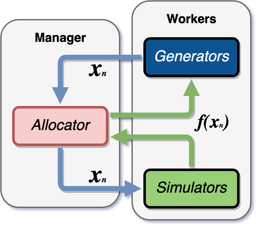
libEnsemble’s workflows are driven by the interoperability between three components referred to as user functions, coordinated by a manager and multiple workers. Generator user functions produce candidate inputs/parameters for simulations or experiments. Simulator functions perform and monitor those simulations or experiments. Allocator functions coordinate data transfer between the generators and simulators and can additionally assign compute resources to user functions or perform additional tasks such as cancelling active simulations based on a request from the generator. libEnsemble’s workers typically launch generator and simulator functions, while the manager handles the allocator function, as depicted in Figure 1. Thousands of concurrent simulator and generator instances can be asynchronously coordinated and tightly coupled together in a namesake ensemble.

User functions are simply Python functions that conform to libEnsemble’s API; that is, they must process their first parameter as an input NumPy[25] array and then return/communicate another array containing results. Between these two steps, any level of computation and complexity is possible. Additional Python libraries can be imported, multinode compiled applications launched and monitored via libEnsemble’s built-in executors, models trained, or any other routine performed. With few exceptions, any kind of computation is possible in libEnsemble’s user functions.

User functions commonly have a state that they wish to maintain and update as results are observed. Such functions can be launched in libEnsemble in a persistent mode, as opposed to a fire-and-forget mode that is commonly used in other workflow packages. This persistent mode is facilitated by user-facing persistent support routines that allow user functions to continuously send and receive intermediate results or additional input parameters while maintaining state. For example, APOSMM[26], a parallel optimization generator function distributed with libEnsemble, persistently maintains and advances multiple local-optimization subprocesses as simulation results are returned to APOSMM in real time.

libEnsemble distributes dozens of example functions and complete workflows as part of its package and online community examples[20]. Users are welcome to browse these examples, distribute or modify them to serve their purposes, and even contribute new examples.

2.1 History Array

libEnsemble’s manager maintains a local NumPy structured array referred to as the history array, which contains a record of all generated and evaluated values and corresponding metadata. Results from each user function are slotted into this array, and inputs into user functions are selected from it. Upon completing a workflow, incrementally, or encountering an error, libEnsemble dumps the history array to file.

Generator functions can preempt, prioritize, or otherwise manipulate the run order of simulations by assigning sim_ids and priority rankings to corresponding output parameters in the history array.

2.2 Generator Functions

Generator functions in libEnsemble play a pivotal role in defining the exploration strategy within the parameter space for simulations or experiments.

Since the possible objectives driving explorations are countless, corresponding generators range from simple designs, such as those requesting batches of randomly sampled points, to substantially more complex methods. For instance, APOSMM coordinates multiple instances of structure-exploiting numerical optimizers. Each optimizer instance may begin its search from a distinct point in the parameter space, leveraging the parallel computing capabilities of libEnsemble to efficiently explore large and complex parameter spaces for simulations that are likely already using (considerable) parallel resources.

The flexibility of generators allows users to tailor their search strategy according to the problem at hand, whether it involves scanning a broad area to identify regions of interest or focusing on refining solutions within one. Moreover, generator functions can dynamically adjust their requests based on real-time output from ongoing simulations. This includes the capability to request the cancellation of currently running simulations if, for example, those simulations are deemed unlikely to give useful output. Cancellation could also be useful if robustness to perturbations in input parameters is desired but there are running simulations using input parameters that are very close to those that have been discovered to crash the simulation. Such cancellation functionality is critical when managing expensive-to-evaluate simulations and computational resources are limited. libEnsemble has been used in this way to limit the number of expensive energy density functional evaluations performed, which has led to additional generator methodology research on how to address such missing output; see, for example, Chan et al.[27].

⬇

import numpy as np

\pardef uniform_random_sample(_, persis_info, gen_specs):

\parub = gen_specs[”user”][”ub”]

lb = gen_specs[”user”][”lb”]

\parn = len(lb)

b = gen_specs[”user”][”gen_batch_size”]

\parOut = np.zeros(b, dtype=gen_specs[”out”])

\parOut[”x”] = persis_info[”RS”].uniform(lb, ub, (b, n))

\parreturn Out, persis_info

Figure 2: Simple random-sampling generator function

Figure 2 illustrates a simple generator that produces $b$ points in the $n$-dimensional box defined by the vectors $lb$ and $ub$ using the random stream $RS$. As this random stream is being stored in the persistent information passed to and from the generator, such an approach not only gives greater control over the random sampling process but also helps ensure that results are reproducible. While random stream management may not be essential for uniform sampling, maintenance of random streams is critical for other generative processes.

2.3 Simulator Functions

The outputs from the generator functions are assumed to be the inputs for the simulator functions. The generator-produced inputs could be meshes used for a computational fluid dynamics simulation, magnet strengths and locations for a synchrotron particle accelerator, or hyperparameters for a convolutional neural network. Simulations can use purely CPU or CPU and GPU resources to perform their computations. Simulator functions can be extremely simple, such as the one in Figure 3, or arbitrarily complex and depend on external executables or non-Python libraries. To make it as easy as possible to interface with such simulators, the libEnsemble executor can be used to launch applications and monitor results.

⬇

import numpy as np

\pardef sim_f(In):

Out = np.zeros(1, dtype=[(”f”, float)])

Out[”f”] = np.linalg.norm(In)

return Out

Figure 3: Synthetic simulator function

2.4 Application Launchers – Executors

libEnsemble features executors for portably launching and monitoring user applications. In stark contrast to the common pattern of Python subprocessing an application instance, libEnsemble’s MPIExecutor builds corresponding MPI run lines based on compute-resource counts, MPI distribution information, scheduler information, and user inputs. This executor is coupled to libEnsemble’s comprehensive resource detection and allocation. For example, an Executor.submit() instruction to launch an application across eight nodes and thirty-two GPUs will not need any adjustment whether libEnsemble is running on Intel, AMD, or Nvidia resources, with any common scheduler or MPI distribution.

libEnsemble’s executors also feature poll, kill, wait, and other functions for monitoring the status of applications. The manager_poll function, in particular, checks for signals relayed by the manager from a generator, enabling generator functions to request the cancellation of already-running applications.

Figure 4: Using Balsam in libEnsemble to run applications across machines

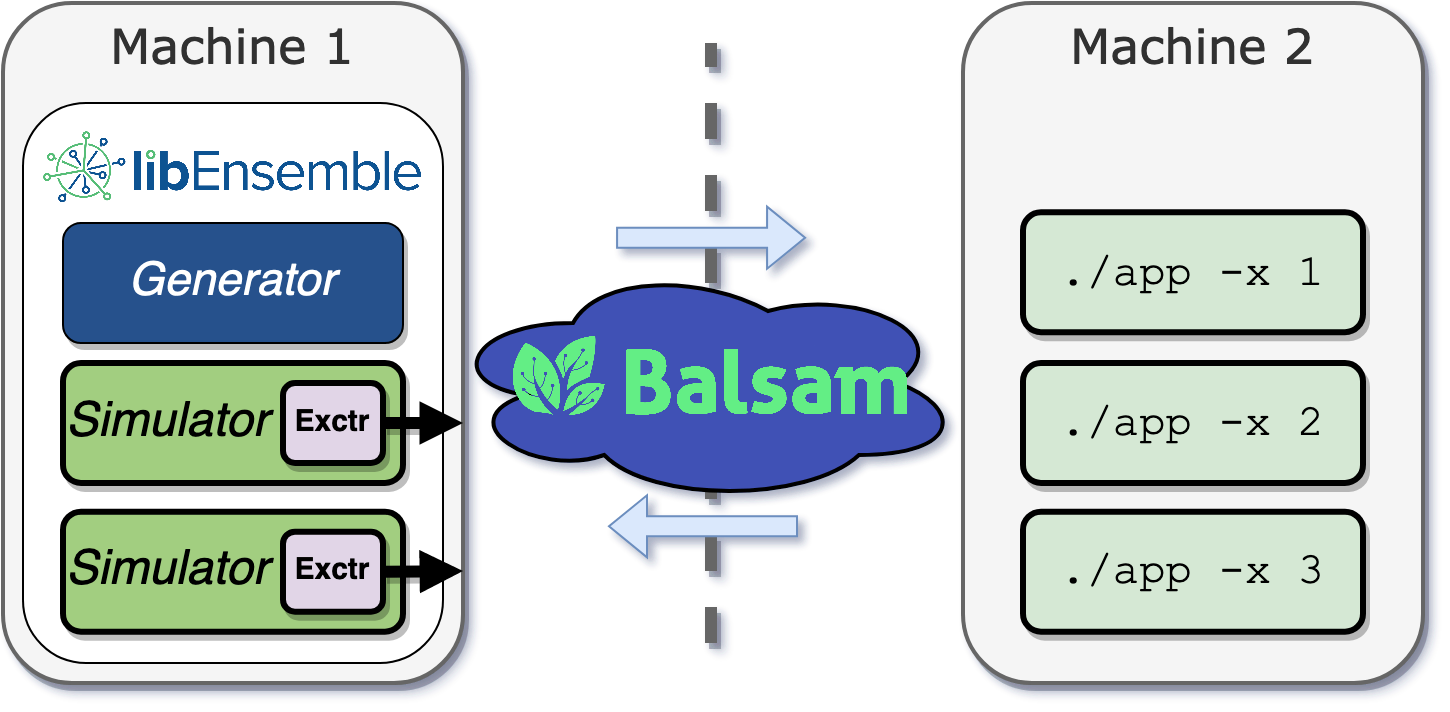
The MPIExecutor can be swapped out with the BalsamExecutor so simulation functions can submit application instances onto separate resources, as depicted in Figure 4, enabling cross-site heterogeneous resource ensembles. This process additionally involves wrapping the application command in Balsam’s ApplicationDefinition class, then running a BalsamExecutor.submit_allocation request to reserve compute resources on the remote system. This system is not tightly coupled to libEnsemble’s local resource management, but the BalsamExecutor can still request variable amounts of compute resources from remote systems, ensuring that dynamically sized application launches are possible.

2.5 Allocator Functions

The allocation function orchestrates the ensemble, deciding whether simulation or generation work should be done as the ensemble progresses, possibly considering the outputs from intermediate calculations. The simplest (and default) libEnsemble allocation function calls the generator function when no simulation work exists and otherwise sequentially gives out previously generated simulation work that has not started to be simulated. While sophisticated generators can observe previous simulation results and adjust their future requests, not all approaches are so advanced. In such cases, the allocation function can have logic to perform such capabilities. The worker array and the history array are central to the allocation functions’ decisions. The worker array gives a snapshot of the currently running activities and the available resources. The history—containing all pending and completed computations performed by workers, including their outputs and run times—enables the allocation function to know the state of the ensemble and to dynamically make decisions about future work. This dynamic decision-making process ensures that the computational resources are used efficiently, prioritizing tasks that are most likely to advance the ensemble’s objectives. It allows for real-time adaptation as the knowledge of the simulation’s landscape improves.

2.6 Simulation Cancellation

The persistent and tightly coupled nature of ensemble members within libEnsemble allows generators to dynamically cancel simulations. This capability is especially valuable when computations are expensive since computational resources may then be used on more critical evaluations as determined by a generator; for example, a faster surrogate model approximates that a slower evaluation may be wasteful. Via persistent functions, generators can both cancel pending simulations and instruct libEnsemble to send kill signals to currently running simulations. Cancellation of simulations is by no means a hard termination; simulation functions are often written to poll for kill signals from the manager, then clean up and kill their applications themselves. libEnsemble includes routines such as Exectutor.polling_loop() to simplify this process. Assigned computational resources are then recovered and reallocated to more valuable computations.

2.7 Running on Multiple Compute Sites

libEnsemble features three approaches for running cross-machine ensembles of computations.

2.7.1 Balsam:

Via Balsam[28], libEnsemble’s user function instances can schedule and launch applications on separate machines, as depicted in Figure 4. This approach separates workflow and application compute resources. User functions can also request and relinquish compute resources on the separate machine for those applications.

2.7.2 Globus Compute:

Via Globus Compute (formerly funcX[11]), libEnsemble’s worker processes can submit their user functions to separate machines. This allows fire-and-forget variants of user functions (usually simulators) to themselves use parallel resources such as MPI or be co-located with their launched applications on the separate machine.

2.7.3 Reverse SSH:

Via a lower-level reverse-SSH interface, libEnsemble can launch its worker processes onto separate machines, effectively splitting the workflow software itself across a network. Persistent user functions launched by remote workers can communicate with libEnsemble’s manager across the network, unlike with Globus Compute; but fewer concurrent worker processes are formally supported.

3 Resource Detection and Management

By default, libEnsemble equally divides available compute resources among workers, and many users running fixed-size simulations do not need to consider dynamic resources. However, libEnsemble has built-in support for dynamic resource allocation. Here, dynamic refers to automatically determining what type/quantity of compute resources to allocate to a given application based on characteristics including run time, power usage, GPU usage, and other performance factors. These resource details are exposed, as stated previously, to libEnsemble’s generators. Via a generalized resource set interface that wraps selections of CPUs, GPUs, and/or nodes as simple enumerations, generators and their underlying algorithms can automatically tune compute resources to simulations in order to find optimal configurations; for example, one could seek to maximize performance subject to a constraint on resource usage.

To support portability, libEnsemble incorporates considerable detection of system information, including scheduler details, MPI runners, core counts, and GPU counts, and uses these to produce run lines and GPU settings for these systems, without the user having to modify scripts. For example, libEnsemble can detect NVIDIA, AMD, and Intel GPUs and uses the detected system information, along with MPI runner/scheduler information, to assign work in an appropriate way for the system, be it command line settings or environment variables such as ROCR_VISIBLE_DEVICES or CUDA_VISIBLE_DEVICES. This means that when simulation input parameters are created, the number of processes and GPUs for each simulation can also be set, and libEnsemble will assign resources correctly for the system.

In some circumstances alternative ways of assigning devices are possible, or multiple MPI runners may be found, and so users can also supply platform settings. The approach here is to honor settings explicitly given, while detecting any that are not given. A list of known platforms, including DOE leadership-class machines, is maintained within libEnsemble; and these can also be specified in user scripts or via an environment variable. However, most of these known systems are also detected automatically.

3.1 Multiapplication Ensembles

The dynamic resource approach allows ensembles that have multiple applications, each using different resources. The multifidelity studies[21, 15] use many fast Wake-T simulations, running on a single CPU core, alongside fewer, highly targeted particle-in-cell (PIC) simulations (e.g., using FBPIC or WarpX), which may use one or more GPUs. This approach has demonstrated a factor of 10 speedup in parameter optimization over the single-fidelity approach. Nodes combine runs of Wake-T and FBPIC, allowing highly efficient resource utilization on each node. While GPU applications often leave many CPU cores idle, the additional CPU cores in this case are used to run Wake-T simulations. Thus a double win is achieved: efficiency is gained by minimizing expensive simulations, and resource efficiency is gained by exploiting the excess CPU cores.

4 Parallelization Methods

libEnsemble supports four methods for initializing parallelization and manager/worker communications. Each method offers various scaling/speed/local-data benefits and trade-offs, and libEnsemble workflows are portable across each method.

4.1 MPI

Running with MPI-based processes typically scales the best, is the most flexible with process placement on multinode systems, and is often the most familiar to scientific users. Launching libEnsemble with MPI is as simple as
mpirun -n 65 python my_libensemble_workflow.py,
which will start one manager process on rank 0 with the remaining being reserved for workers. Other related MPI runners on clusters, such as aprun or srun, can also be used. Internally libEnsemble coerces runtime information and communicates via mpi4py[29] methods.

4.2 Multiprocessing

Referred to as local communications, the multiprocessing mode uses Python’s standard library multiprocessing module to start separate Python interpreters/processes for workers, then communicate via queues from the same module. Each process is initialized on the same node, either a launch node or a single compute node. The remaining nodes allocated within a job are accessible via libEnsemble’s executors for launching applications (workers and applications are not co-located).

4.3 Threading

The threading mode starts separate threads for each worker from Python’s standard library threading module. This communication mode has the same locality limitations as multiprocessing. Other major limitations are that the resource allocation process is not thread safe and workers cannot maintain separate working directories.

The benefits are that workers can both access shared data structures and communicate via reference; this mode is significantly faster and ensures that models or other objects supplied to workers are updated in place (not copied). For example, a generator’s state is updated in place and is immediately accessible to the manager.

We note that Python-level code is not technically parallel because of Python’s global interpreter lock (GIL). However, libraries such as NumPy, used throughout libEnsemble, offload computational heavy lifting to compiled code that bypasses the GIL.

Because of the limitations, this communications mode is not generally recommended, but it has proven useful to some users and has been used in live experiments, where libEnsemble is run through a Jupyter notebook.

Currently this mode is recommended only for simple use cases, but it is under active development. We expect that a thread-safe resources implementation will be added in the near future.

4.4 TCP

TCP mode starts separate interpreters on SSH-accessible target systems for each worker via a reverse-SSH interface. Workers communicate back to libEnsemble’s manager via a multiprocessing.Manager. This mode is a lower-level cross-system ensemble approach compared with other solutions such as Globus Compute; similarly, adaptive resource management is not applicable. Uniquely, persistent user functions can be used.

5 Case Study: Online Learning of a Plasma Accelerator

We now use libEnsemble to construct a surrogate model of a laser-plasma interaction using domain-specific simulation codes (WarpX and Wake-T), specifically focusing on the shape of a density down-ramp profile of a plasma accelerator stage over a five-dimensional parameter space. This approach capitalizes on the scalable capabilities of libEnsemble due to the arbitrary concurrency available when exploring a parameter space. The plasma accelerator use case being modeled features a Gaussian density bump as a plasma lens to focus the beam[30]. The objective function is a measure of beam divergence.

For the generator we use gpCAM[31], which implements function approximation and optimization using a Gaussian process, a type of statistical surrogate model[32]. gpCAM is a highly customizable package for autonomous experimentation[33] that supports methods for parallel training, especially for exact (i.e., interpolating) Gaussian processes[34].

For this study we use two simulation codes: WarpX and Wake-T. WarpX is a PIC simulation code that is used to model the problem in 3D (the domain here is decomposed in the $z$-dimension along the beam). It uses MPI parallelism, where each MPI task uses a GPU. The problem is configured to run using 48 GPUs, and it runs for approximately 15–20 minutes on Perlmutter. The objective function of interest for WarpX is the product of the beam divergence in the horizontal (x) and vertical (y) dimensions orthogonal to the beam; the Wake-T simulation is axisymmetric, and the beam divergence is taken in the x direction only.

Wake-T (the Wakefield particle Tracker)[35] is used as a simplified serial code that uses a Runge–Kutta solver to track the evolution of the beam electrons. Wake-T is used here to help configure gpCAM and to measure the overheads of libEnsemble using many workers.

5.1 Motivation for Surrogate Model

Building a surrogate for a plasma-based accelerator stage can help facilitate numerous research and optimization tasks for future designs of high-energy physics colliders that are based on the succession of hundreds to thousands of such stages. Various simulation codes that are used for the modeling of stages, from fast (e.g., the reduced dimensionality with the code Wake-T) to more detailed and more computationally demanding (e.g., fully three-dimensional modeling with WarpX), can be used to build such surrogates. A high-quality global surrogate model of Wake-T and/or WarpX output (over some portion of parameter space) that can sufficiently approximate a specific simulation scenario will enable researchers to conduct extensive collider design experimentation and analysis at a fraction of the time and computational cost. This is particularly advantageous for collider designs where a wide array of scenarios and objectives is to be considered. Such studies enable insights that might not have been initially considered, including designs under various regimes of uncertainty. Such surrogate models will therefore likely be useful for innovation and robustness in particle accelerator applications.

5.2 Online Gaussian Process Training with gpCAM

The aim is to sample the parameter space in areas of maximum uncertainty to construct a Gaussian process surrogate model. Relative to offline/fixed-sample training, this kind of online learning, wherein the input parameters are sequentially selected based on a growing set of training data, can significantly reduce the number of simulation runs required to achieve a level of predictive accuracy. The gpCAM generator is initially run with random points drawn uniformly from the parameter space. The simulation output from this initial set is used to train the Gaussian process surrogate model. Following this initial phase, the 5D parameter space is divided into a mesh of candidate points. The mesh used in the following case was 10 points in each dimension (hence $10^{5}$ points). The input x and the objective function f are used to sample the posterior covariance from gpcAM at each of these candidate points. Noise is initialized to approximately 1% of the mean f value.

With points ranked by their uncertainty (i.e., highest covariance), we select the top-ranked candidate point for sampling. To ensure sampling is spaced out across the parameter space, we proceed by identifying subsequent points that are at a minimum distance r away from previously selected points. This iterative selection is refined by initially setting a substantial value for r and gradually reducing it, allowing us to assemble a batch of simulation points that maintain a minimum separation of r. This strategy ensures both targeted exploration of high-uncertainty regions and spatial diversity within the batch. Once a desired batch size has been reached, simulation outputs are obtained for the entire batch, and the Gaussian process surrogate model is retrained by using the now larger set of training data. This iterative process then repeats, with inputs and their corresponding outputs being obtained in an online manner. libEnsemble has been used in a similar fashion for online Bayesian calibration[36].

Figure 5: Behavior of Wake-T mean squared error as more training data is obtained (simulation input parameters chosen from a uniform random sample (left) and gpCAM (right) of parameter space).

To assess whether the surrogate is improving, we monitor the maximum and mean variance across the candidate points and the mean squared error (MSE) against a test set (i.e., a separate set of sampled points). We do not necessarily expect to see monotonic improvement since the model-computed signal variance—an indicator of the objective function’s unpredictability—may increase if unexpected behavior of the objective is encountered. Nonetheless, our expectation is that, with ongoing sampling and refinement of the model, both the variance indicators and the MSE will demonstrate a general downward trend, indicating enhanced model accuracy and reliability as more model training data is obtained.

5.3 Training Details

The platforms used were Perlmutter (NERSC) and Frontier (OLCF). Both platforms have demonstrated the scalability of WarpX and have been used extensively with libEnsemble[37]. Perlmutter also has a CPU partition that is suitable for use with the Wake-T version.

To prepare the workflow and configure gpCAM, we first use a Wake-T axisymmetric model in place of the 3D WarpX. Since this runs on a single CPU core, it can be run either via libEnsemble’s executor or directly in Python via a function call. For our purposes, a direct function call is sufficient and minimizes overhead. libEnsemble is run with the mpi4py communications option to spread workers across nodes. The use of 32 workers per node was found to scale well up to 2,048 workers (64 nodes). This workflow is used to configure the gpCAM generator and to measure and optimize model training, which can later be adapted to the WarpX workflow.

The full training of the Gaussian process takes nontrivial time, and this time increases as the number of evaluated points given to the model increases. Since we are working with batches, this means that worker resources will be delayed waiting for the Gaussian process to be retrained. A few approaches can be used to improve this situation.

1. Only perform the necessary training at each step. One can assess the quality of the model and perform a full global training (120 iterations), a reduced global training (20 iterations), or a local training, depending on the model quality.

2. Employ different training methods. Markov chain Monte Carlo samples from a probability distribution based on constructing a Markov chain may lead to more robust and reliable modeling in some scenarios.

3. Overlap training with evaluations. libEnsemble supports asynchronous return of evaluations to the generator. This enables overlap of training based on returned evaluations, while concurrently continuing with further evaluations.

4. Use more resources for training. The gp2Scale feature of gpCAM supports parallel training via Dask[38]. This would need to be incorporated into the libEnsemble framework or use existing libEnsemble capabilities (this may entail using the libEnsemble executor within the generator to assign more resources for training).

The first strategy enhances the efficiency of model training by making more judicious decisions on training the model. By default, gpCAM conducts a global training consisting of 120 iterations. We refer to this as full training. Once a robust model is established, reducing the number of iterations for global training becomes feasible. Additionally, transitioning to even faster local training (considering only the local Gaussian process hyperparameter region) becomes an option, offering a more targeted approach to refine the model.

The quality of the model can be assessed by comparing evaluation results predicted by the model with the actual results returned in the last batch. This is similar to the use of test points to measure model quality. In this case we use the gpCAM function rmse (root mean squared error), and we assess the quality of the model to assign training by comparing rmse against the standard deviation of f via the logic shown below.

⬇

rmse = gp.rmse(x_new, y_new)

gp.tell(all_x, all_y)

if rmse > 10.*np.std(all_y):

gp.train(method=’global’, max_iter=120)

elif rmse > 2.*np.std(all_y):

gp.train(method=’global’, max_iter=20)

else:

gp.train(method=’local’)

The above training thresholds, for this use case, provide sufficient training to ensure the model quality remains good enough to keep the variance (and error at test data) trending downward. The time spent training is reduced but would still become a bottleneck as larger numbers of evaluations are returned.

5.4 Results for gpCAM with Wake-T

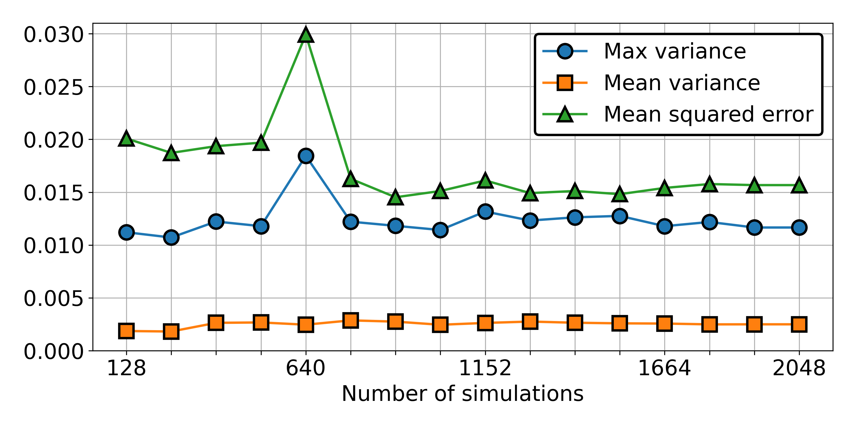
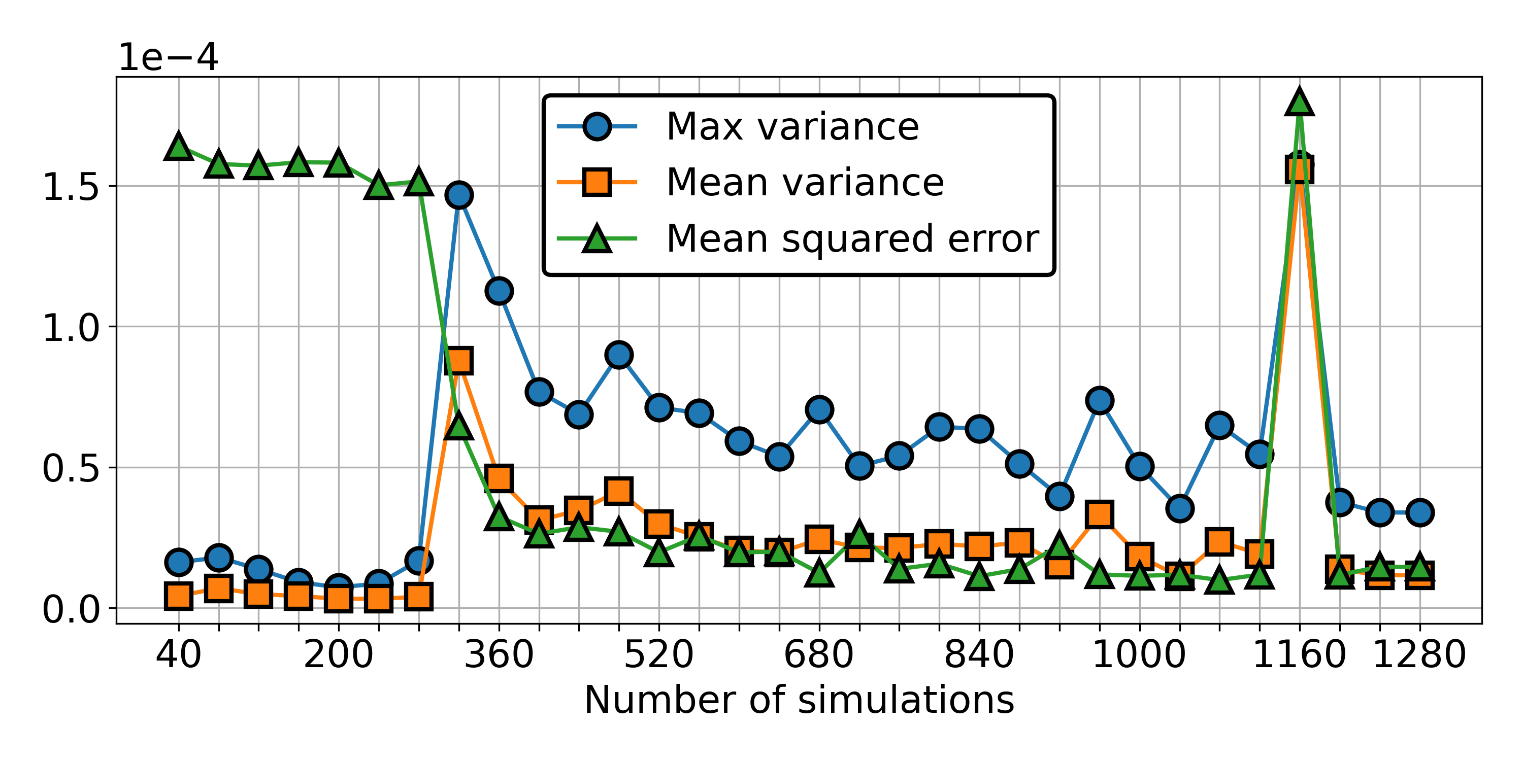
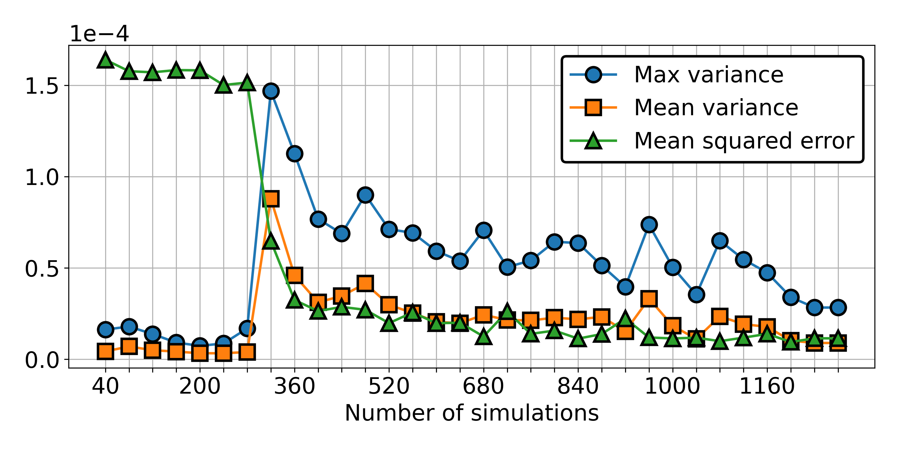
Figure 5 shows the mean squared error at the test points at each iteration of the generator. The graphs also show the mean and maximum variance (posterior covariance) over the grid, as determined by gpCAM. These runs used batches of 128 concurrent evaluations (using 128 workers for running simulations and one worker for the persistent generator function).

Figure 5(left) shows a run where uniformly random points were selected for evaluation and gpCAM was used only to evaluate the posterior mean (for mean squared error) at the test points and posterior variance over the grid of candidate points. This illustrates that while the mean variance of the model stays relatively stable, the maximum variance shows that areas of high uncertainty remain, indicating the existence of potentially underexplored regions. The mean squared error at the test points, with the exception of one spike, also remains roughly constant over this range of number of simulations performed.

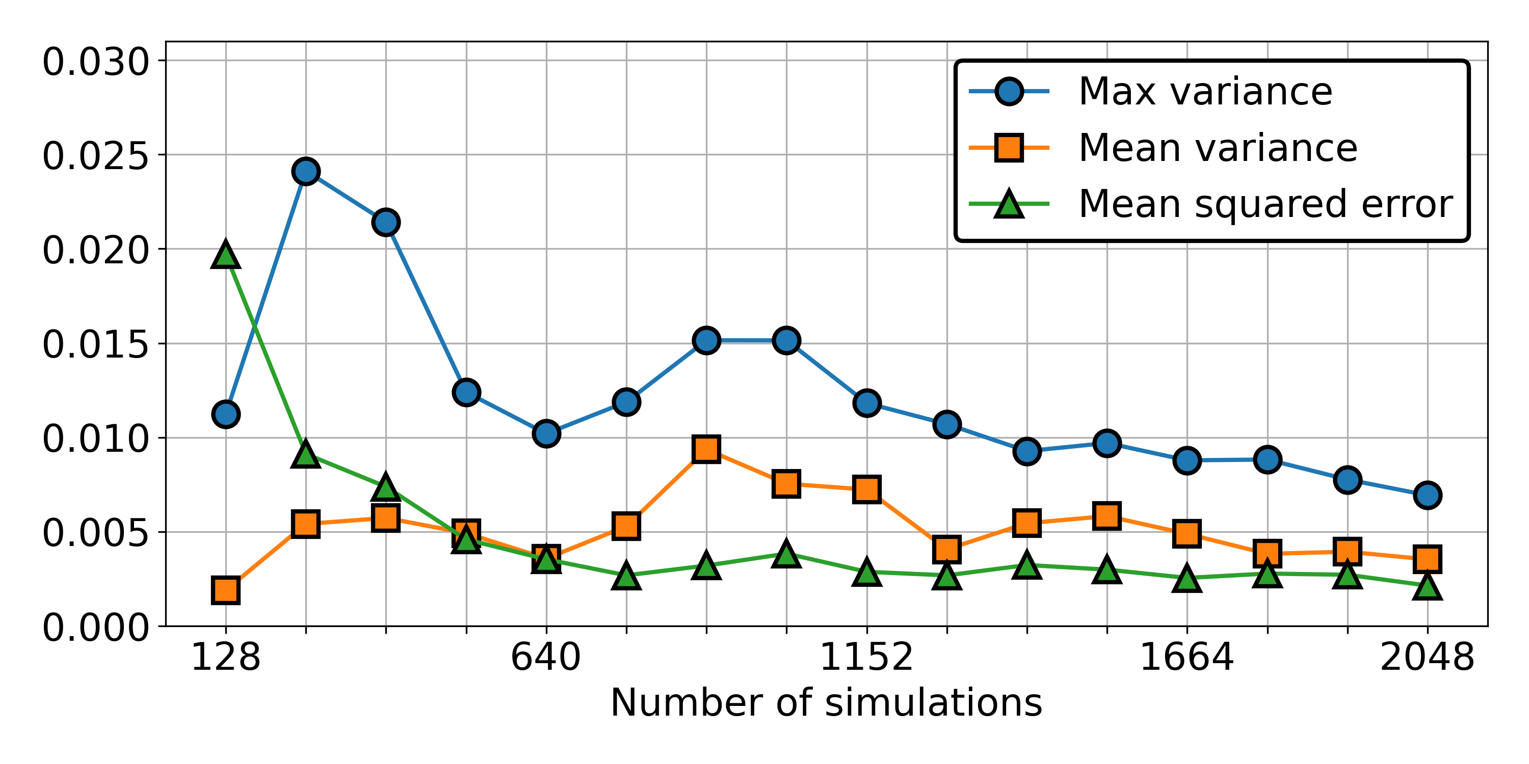
Figure 5(right) shows results when the candidate points are selected using information from gpCAM via the online method described above. The results show that both the mean squared error at the test points and the maximum/mean variance over the grid of candidate points all trend downward over time. The results confirm the expectation that gpCAM is enabling efficient training of the surrogate model.

5.5 Performance Considerations and Scaling

Since the time taken to train the Gaussian process model and query the posterior covariance across the grid of points increases with the number of evaluations, ongoing work will explore the capabilities in gpCAM for more efficient training strategies and for parallelization of training using gp2scale.

During this study we consider using CRPS (Continuous Rank Probability Score) in place of the RMSE as a metric for evaluating model performance and, therefore, training requirements. While RMSE looks only at prediction error, which may be a limited measure in sparse scenarios, CRPS takes the model’s uncertainty estimates into account and therefore may give a better indication of model confidence. Applying the same comparisons using CRPS in place of RMSE resulted in considerably more local retraining, which is significantly faster. However, there were also more frequent spikes in the variance suggesting this training may have been insufficient. We expect that refining the thresholds for different training options (relative to the standard deviation of the objective) will likely make CRPS a more efficient training strategy. This is left for future work. A comparison of Gaussian process hyperparameters used in gpCAM may also be used to make more informed training decisions.

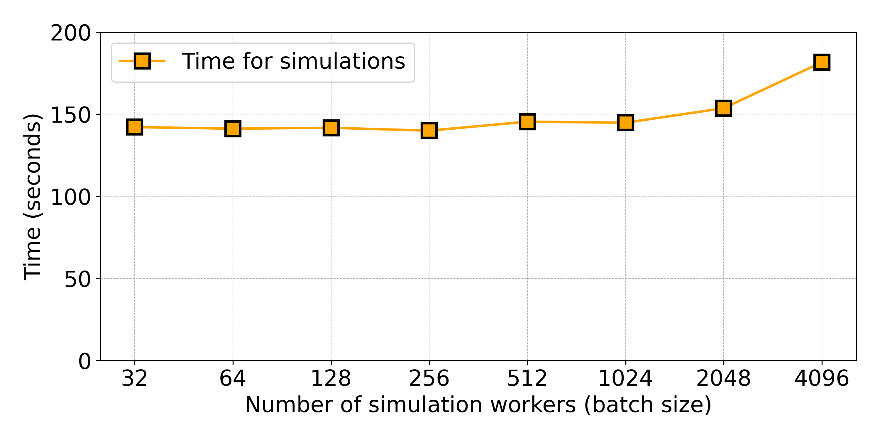
Wake-T run times recorded inside the simulator, from 3,072 runs, average 137.1 seconds with a maximum of 144.7 seconds on the Perlmutter CPU partition using 32 workers per node. To assess the scaling of libEnsemble’s infrastructure, timing is placed around the send/receive call inside the persistent generator function. This timing includes all overhead (including communication between the generator and manager and between manager and simulation workers in addition to time spent in simulations).

Figure 6 shows the timing obtained from the generator from one node (32 simulation workers) doubling up to 4,096 simulation workers. The data shows negligible overhead and nearly perfect speedup to 1,024 workers (98.2% parallel efficiency relative to 32 workers), small overhead at 2,048 workers (92.5% parallel efficiency), and significant overhead at 4,096 workers (78.2%). This demonstrates the high-quality scalability of the mpi4py communications method.

Note that the ability to run the generator on the manager is currently being added to libEnsemble (either in place or on a thread), which may reduce the communication overhead further.

Figure 6: Wake-T weak scaling: Time for one batch of simulations measured by the generator. Note that the number of simulations is equal to the number of workers, hence showing weak scaling.

5.6 WarpX Study

The WarpX version of the downramp simulation has been configured to run on 48 MPI tasks, each using one GPU. This setup is considered the minimum configuration that yields results with an acceptable physical accuracy.

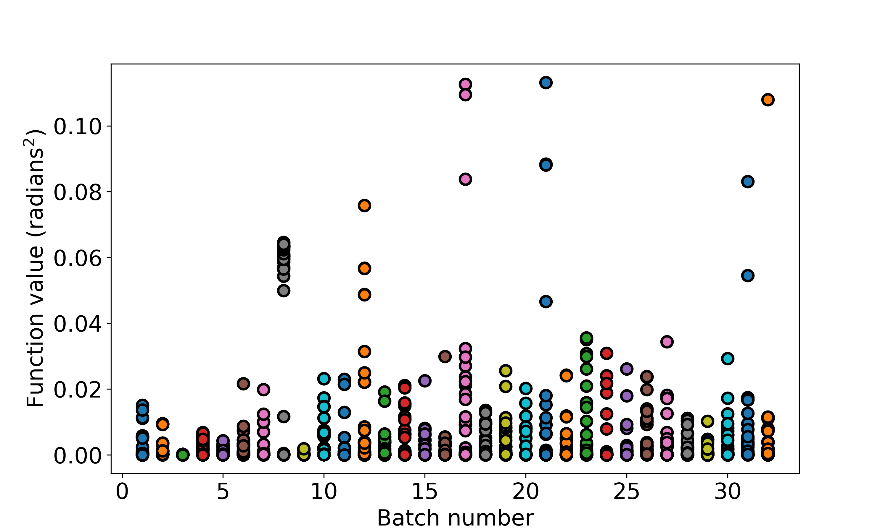
This means that on Perlmutter, each simulation, and hence each worker, uses 12 nodes (in contrast to 32 workers per node for Wake-T). If the number of parallel simulations was scaled to the same extent as the Wake-T study, 27 Perlmutters would be required. In fact, a full Perlmutter run for WarpX would use only 149 workers. On Frontier, there are eight GPUs per node, and hence each simulation requires only six nodes. On both systems, the WarpX run time is similar—approximately 800 seconds. On Perlmutter, however, about one run in 40 ran slowly and took up to 2,000 seconds. The reason for this is not clear, but the decision was taken to kill simulations that took longer than 1,000 seconds in order not to waste resources in a batched scenario. This is achieved through libEnsemble’s executor interface, which has a portable kill function. The killed simulations return NaNs, which are excluded in the generator. Frontier, however, did not experience these slow runs. For these reasons, Frontier was favored for a large ensemble using WarpX. Figure 7 shows the results of running 32 iterations with a batch size of 40 on Frontier (a total of 240 nodes).

Figure 7: Behavior of WarpX mean squared error as more training data is obtained (simulation input parameters chosen by gpCAM process).

5.7 WarpX Results

The mean squared error at the test points shows a downward trend with a steep improvement between batches seven and nine. The model appears to start with fairly low uncertainty estimates; on processing, however, the eighth batch shows an increase in uncertainty but a reduction in error, suggesting an improvement of the surrogate. This corresponds with hitting some much larger objective values (shown in Figure 8).

Figure 8: WarpX objective function value distribution by batch.

A spike occurs in the mean squared error and variance after 29 batches. This spike does not correspond to encountering obviously wayward values for the objective or to the RMSE for the last batch of points. However, examining the Gaussian process hyperparameters used in gpCAM shows that the length scale hyperparameter for the bump width is less than one-tenth of the range in this dimension, which may make the model oversensitive.

The RMSE-directed training resulted in 10 full global training iterations, 20 smaller global training iterations, and one local training.

The occurrence of the spike in variance (and mean squared error) was observed to be in close proximity to the single instance of local training. Thus a second run was conducted on Frontier where the local training option was removed, thereby ensuring that either full or reduced global training was carried out by gpCAM. This second run, shown in Figure 9, does not result in the aforementioned spike. Future efforts will be directed toward developing strategies to more effectively handle anomalies in the Gaussian process hyperparameter values.

Figure 9: Behavior of WarpX mean squared error when gpCAM always performs global training (simulation input parameters chosen by gpCAM process).

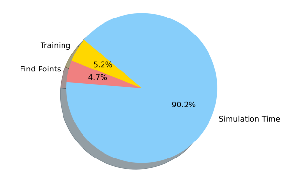
The overall time taken in this second run as measured from the generator function in training the model, selecting points (including measuring posterior covariance, sorting, and determining best points), and running simulations (including communication) is shown in Figure 10. The overhead from manager-worker communications was negligible.

Figure 10: Time spent in training the model, deciding new points, and running WarpX simulations on Frontier ensemble

5.8 Summary of Surrogate Case Study

In summary, we were able to show progression toward a predictive surrogate model with both Wake-T and WarpX for the given use case. The lower-fidelity code (Wake-T) might not capture all of the physics, but it gives an initial understanding of the system response over the parameter space. WarpX captures more of the physics and while a sensitivity to training choices was observed, the mean squared error at the validation points trends downward, and several avenues for further configuration of the training protocol are available.

We demonstrated near-perfect weak scaling of libEnsemble’s mpi4py communications to over a thousand workers on Perlmutter (a relative parallel efficiency of 98.2% for 1,024 workers to 32 workers).

As long as the processing time spent in the generator remains minimal or is overlapped with simulations, extensive computational resources can be utilized for building such surrogate models. A full system run of the WarpX use case on Frontier would use 1,568 workers (9,408 nodes with six nodes per worker), which is within the scaling range demonstrated by the Wake-T use case, with a global parallel efficiency close to that of each individual simulation.

libEnsemble has also been tested and shown to scale well on the Aurora supercomputer at the Argonne Leadership Computing Facility. Once WarpX has been successfully ported to Aurora, this is also expected to be a good system for further studies.

6 Future Work

libEnsemble is in active development and has a growing community of users. Its generalized interface lends it well to cutting-edge research across a large variety of disciplines and experimental use cases. We consider the following to be especially worthy of further investigation.

6.1 Manager-Run Generator

Generator user functions within libEnsemble have always been the responsibility of the worker processes to launch and handle. However, for common use cases involving only a single generator instance, placing that generator on a worker process introduces inherent communication and process overheads that could be sidestepped by keeping that generator local to the manager process. Furthermore, user input data would be available for the generator to read/write by reference, exposing partial benefits of libEnsemble’s threading parallelism to the MPI and multiprocessing methods.

6.2 Using libEnsemble for Simulation Dispatch

libEnsemble’s in-the-loop generator facilitates close coupling of generators and simulators, especially in asynchronous scenarios. However, some users may wish to exploit libEnsemble’s capabilities with an external generator. While doing so is possible, a concurrent/futures interface that allows libEnsemble to be used as a dispatch engine for simulations may better suit the needs of some users.

6.3 Worker-Side Resource Management

Another characteristic of the current resource implementation is that the manager controls resources and assigns these to workers. An alternative scheme is to manage resources on the worker side. Under this model, workers could use an alternative executor to dispatch tasks to a dedicated process that would assign resources and submit application runs. This method could leverage much of the existing resource management and submission infrastructure.

6.4 Improved Domain Support

While libEnsemble’s generalized interface is an advantage in adapting it to a wide variety of use cases, some users (e.g., the developers of Optimas) have developed higher-level libraries that wrap libEnsemble for specific disciplines. As the amount of artificial intelligence and machine-learning applications increases, libEnsemble can likewise serve that domain by exposing high-level Model.train test, ask, tell, or other general functions.

Furthermore, AI/ML is also supported by improving multisite capabilities; the libEnsemble team is highly interested in coordinating ensembles simultaneously across supercomputers and AI testbeds with special-purpose accelerators.

6.5 Data Streaming

libEnsemble’s traditional data communications have been restricted to points, often single NumPy arrays that must be communicated between the workers via the manager; in practice for large amounts of data, this approach is relatively slow and inefficient. This could be improved by sending a proxy or stream handle via the manager (e.g., using ProxyStore[39]), to transparently stream data directly between workers.

6.6 Portable Generator Interface

libEnsemble’s user functions are currently constructed to be launched and processed by libEnsemble only. This produces advantages such as ensuring that useful libEnsemble data structures are available within such functions, guaranteeing they are portable across every libEnsemble version, and not forcing users to adhere to any specific design patterns except input/output types. However, as the ecosystem of generator-algorithm studies and upstream software that depends on libEnsemble grows, so does the request for libEnsemble to also launch and process third-party generators. This is currently supported via writing wrapper user functions, although this wrapper code often fits design patterns that libEnsemble could handle on the user’s behalf.

Initial efforts indicate that many third-party generative interfaces consist of .ask() and .tell() (or .read() and .update()) functions. libEnsemble’s workers could potentially interleave calling such functions with sending/receiving corresponding data from libEnsemble’s manager. Furthermore, if libEnsemble’s traditional generators were also reconstructed with that two-function paradigm, they would be available for use in other workflow packages.

7 Acknowledgements

This article was supported in part by the PETSc/TAO activity within the U.S. Department of Energy’s (DOE’s) Exascale Computing Project (17-SC-20-SC) and by the CAMPA, ComPASS, and NUCLEI SciDAC projects within DOE’s Office of Science, Advanced Scientific Computing Research under contract numbers DE-AC02-06CH11357 and DE-AC02-05CH11231. We acknowledge contributions from David Bindel early in libEnsemble’s development. We thank Marco Garten, Remi Lehe, Jean-Luc Vay, Ángel Ferran Pousa, and Axel Huebl for supplying Wake-T and WarpX use cases. We thank Marcus Noack for assistance with gpCAM.

This research used resources of the Oak Ridge Leadership Computing Facility, a DOE Office of Science User Facility supported under Contract DE-AC05-00OR22725, and the National Energy Research Scientific Computing Center (NERSC), a DOE Office of Science User Facility located at Lawrence Berkeley National Laboratory and operated under Contract DE-AC02-05CH11231 using NERSC awards ASCR-ERCAP0028863 and HEP-ERCAP0027030.

Biographies of the authors

Stephen Hudson received his M.Sc. (2001) in computer science from Oxford Brookes University. He is a software engineer and numerical library developer in LANS, the Laboratory for Applied Mathematics, Numerical Software, and Statistics, at Argonne National Laboratory. He specializes in high-performance computing.

Jeffrey Larson received his B.A. (2005) in mathematics from Carroll College and his M.S. (2008) and Ph.D. (2012) in applied mathematics from the University of Colorado Denver. He is a computational mathematician in LANS, the Laboratory for Applied Mathematics, Numerical Software, and Statistics, at Argonne National Laboratory. He studies algorithms for optimizing computationally expensive functions arising in quantum information science, fusion power plant and particle accelerator design/operation, and vehicle routing.

John-Luke Navarro received his B.A. (2018) in computer science from Andrews University. He is a software engineer in LANS, the Laboratory for Applied Mathematics, Numerical Software, and Statistics, at Argonne National Laboratory.

Stefan M. Wild received B.S. and M.S. degrees in applied mathematics from the University of Colorado in 2003 and a Ph.D. degree in operations research from Cornell University in 2009. He is a senior scientist and director of the Applied Mathematics and Computational Research Division at Lawrence Berkeley National Laboratory. He is an adjunct faculty in Industrial Engineering and Management Sciences at Northwestern University. His research interests include the development of formulations, algorithms, and software for challenging mathematical optimization problems.

The submitted manuscript has been created by UChicago Argonne, LLC, Operator of Argonne National Laboratory (“Argonne”). Argonne, a U.S. Department of Energy Office of Science laboratory, is operated under Contract No. DE-AC02-06CH11357. The U.S. Government retains for itself, and others acting on its behalf, a paid-up nonexclusive, irrevocable worldwide license in said article to reproduce, prepare derivative works, distribute copies to the public, and perform publicly and display publicly, by or on behalf of the Government. The Department of Energy will provide public access to these results of federally sponsored research in accordance with the DOE Public Access Plan http://energy.gov/downloads/doe-public-access-plan.

References

- [1] Hudson S, Larson J, Navarro JL et al. libEnsemble: A library to coordinate the concurrent evaluation of dynamic ensembles of calculations. IEEE Transactions on Parallel and Distributed Systems 2022; 33(4): 977–988. doi:10.1109/tpds.2021.3082815.
- [2] Hudson S, Larson J, Navarro JL et al. libEnsemble: A complete Python toolkit for dynamic ensembles of calculations. Journal of Open Source Software 2023; 8(92): 6031. doi:10.21105/joss.06031.
- [3] Hudson S, Larson J, Wild SM et al. libEnsemble, 2024. URL https://github.com/Libensemble/libEnsemble.
- [4] Hudson S, Larson J, Wild SM et al. libEnsemble users manual, 2022. URL https://buildmedia.readthedocs.org/media/pdf/libensemble/latest/libensemble.pdf.
- [5] Balasubramanian V, Treikalis A, Weidner O et al. Ensemble toolkit: Scalable and flexible execution of ensembles of tasks. In 2016 45th International Conference on Parallel Processing. IEEE. doi:10.1109/icpp.2016.59.
- [6] Ward L, Sivaraman G, Pauloski JG et al. Colmena: Scalable machine-learning-based steering of ensemble simulations for high performance computing. In IEEE/ACM Workshop on Machine Learning in High Performance Computing Environments. pp. 9–20. doi:10.1109/MLHPC54614.2021.00007.
- [7] Moritz P, Nishihara R, Wang S et al. Ray: A distributed framework for emerging AI applications, 2018. doi:10.48550/arXiv.1712.05889.
- [8] Cunningham W. AgnostiqHQ/covalent: v0.228.0-rc.0, 2023. doi:10.5281/zenodo.5903364.
- [9] Balay S, Abhyankar S, Adams MF et al. PETSc/TAO users manual. Technical Report ANL-21/39 - Revision 3.20, Argonne National Laboratory, 2023. doi:10.2172/2205494.
- [10] Hategan-Marandiuc M, Merzky A, Collier N et al. PSI/J: A portable interface for submitting, monitoring, and managing jobs. In 2023 IEEE 19th International Conference on e-Science. pp. 1–10. doi:10.1109/e-Science58273.2023.10254912.
- [11] Chard R, Babuji Y, Li Z et al. funcX: A federated function serving fabric for science. In Proceedings of the 29th International Symposium on High-Performance Parallel and Distributed Computing. pp. 65–76. doi:10.1145/3369583.3392683.
- [12] Bartlett R, Demeshko I, Gamblin T et al. xSDK foundations: Toward an extreme-scale scientific software development kit. Supercomputing Frontiers and Innovations: an International Journal 2017; 4(1): 69–82. doi:10.14529/jsfi170104.
- [13] Neveu N, Hudson S, Larson J et al. Comparison of model-based and heuristic optimization algorithms applied to photoinjectors using libEnsemble. In Proceedings of the 13th International Computational Accelerator Physics Conference. pp. 22–24. doi:10.18429/JACoW-ICAP2018-SAPAF03.
- [14] Neveu N, Chang TH, Franz P et al. Comparison of multiobjective optimization methods for the LCLS-II photoinjector. Computer Physics Communications 2023; 283: 108566. doi:10.1016/j.cpc.2022.108566.
- [15] Ferran Pousa A, Jalas S, Kirchen M et al. Multitask optimization of laser-plasma accelerators using simulation codes with different fidelities. In Proceedings of the 13th International Particle Accelerator Conference. doi:10.18429/JACoW-IPAC2022-WEPOST030.
- [16] Chang TH, Larson J, Watson LT et al. Managing computationally expensive blackbox multiobjective optimization problems with libEnsemble. In Proceedings of the Spring Simulation Conference. doi:10.22360/springsim.2020.hpc.001.
- [17] Plumlee M, Sürer O, Wild SM et al. surmise 0.2.1 users manual. Technical Report Version 0.2.1, NAISE, 2023. URL https://surmise.readthedocs.io.
- [18] Chan MY. High-Dimensional Gaussian Process Methods for Uncertainty Quantification. PhD Thesis, Northwestern University, 2023.
- [19] Wu X, Tramm J, Larson J et al. Integrating ytopt and libEnsemble to autotune OpenMC, 2024. doi:10.48550/arXiv.2402.09222.
- [20] libEnsemble Community. A selection of libEnsemble functions and complete workflows from the community, 2023. URL https://github.com/Libensemble/libe-community-examples.
- [21] Ferran Pousa A, Jalas S, Kirchen M et al. Bayesian optimization of laser-plasma accelerators assisted by reduced physical models. Physical Review Accelerators and Beams 2023; 26: 084601. doi:10.1103/PhysRevAccelBeams.26.084601.
- [22] Chang TH and Wild SM. ParMOO: A Python library for parallel multiobjective simulation optimization. Journal of Open Source Software 2023; 8(82): 4468. doi:10.21105/joss.04468.
- [23] Chang TH and Wild SM. Designing a framework for solving multiobjective simulation optimization problems. Technical Report 2304.06881, arXiv, 2023. URL https://arxiv.org/abs/2304.06881.
- [24] RadiaSoft. rsopt, 2024. URL https://github.com/radiasoft/rsopt.
- [25] Harris CR, Millman KJ, van der Walt SJ et al. Array programming with NumPy. Nature 2020; 585(7825): 357–362. doi:10.1038/s41586-020-2649-2.
- [26] Larson J and Wild SM. Asynchronously parallel optimization solver for finding multiple minima. Mathematical Programming Computation 2018; 10(3): 303–332. doi:10.1007/s12532-017-0131-4.
- [27] Chan MYH, Plumlee M and Wild SM. Constructing a simulation surrogate with partially observed output. Technometrics 2024; 66(1): 1–13. doi:10.1080/00401706.2023.2210170.
- [28] Salim MA, Uram TD, Childers JT et al. Balsam: Automated scheduling and execution of dynamic, data-intensive HPC workflows, 2019. doi:10.48550/arXiv.1909.08704.
- [29] Dalcin L and Fang YLL. mpi4py: Status update after 12 years of development. Computing in Science & Engineering 2021; 23(4): 47–54. doi:10.1109/MCSE.2021.3083216.
- [30] Thaury C, Guillaume E, Döpp A et al. Demonstration of relativistic electron beam focusing by a laser-plasma lens. Nature Communications 2015; 6(1). doi:10.1038/ncomms7860.
- [31] Noack M, Sethian J, Yager K et al. gpcam, 2023. doi:10.5281/zenodo.10393189.
- [32] Gramacy RB. Surrogates: Gaussian Process Modeling, Design and Optimization for the Applied Sciences. Boca Raton, Florida: Chapman Hall/CRC, 2020. doi:10.1201/9780367815493.
- [33] Noack M and Ushizima D. Methods and Applications of Autonomous Experimentation. Chapman and Hall/CRC, 2023. doi:10.1201/9781003359593.
- [34] Noack MM, Krishnan H, Risser MD et al. Exact Gaussian processes for massive datasets via non-stationary sparsity-discovering kernels. Scientific Reports 2023; 13(1): 3155. doi:10.1038/s41598-023-30062-8.
- [35] Ferran Pousa A, Assmann R and Martinez de la Ossa A. Wake-T: A fast particle tracking code for plasma-based accelerators. Journal of Physics: Conference Series 2019; 1350(1): 012056. doi:10.1088/1742-6596/1350/1/012056.
- [36] Sürer O, Plumlee M and Wild SM. Sequential Bayesian experimental design for calibration of expensive simulation models. Technometrics 2024; doi:10.1080/00401706.2023.2246157. To appear.
- [37] Fedeli L, Huebl A, Boillod-Cerneux F et al. Pushing the frontier in the design of laser-based electron accelerators with groundbreaking mesh-refined particle-in-cell simulations on exascale-class supercomputers. In SC22: International Conference for High Performance Computing, Networking, Storage and Analysis. pp. 1–12. doi:10.1109/SC41404.2022.00008.
- [38] Rocklin M. Dask: Parallel computation with blocked algorithms and task scheduling. In Proceedings of the Python in Science Conference. SciPy. doi:10.25080/majora-7b98e3ed-013.
- [39] Pauloski JG, Hayot-Sasson V, Ward L et al. Accelerating communications in federated applications with transparent object proxies. In Proceedings of the International Conference for High Performance Computing, Networking, Storage and Analysis. SC ’23, New York, NY, USA: Association for Computing Machinery. doi:10.1145/3581784.3607047.