Universality of pseudo-Goldstone damping near critical points

Abstract

In recent studies of holographic models and hydrodynamics with spontaneous breaking of approximate symmetries, it has been proposed that the damping of pseudo-Goldstone modes at finite temperatures is universally constrained in the way that $\Omega_{\varphi}/m_{\varphi}^{2}\simeq D_{\varphi}$ in the broken phase, where $\Omega_{\varphi}$ and $m_{\varphi}$ are the relaxation rate at zero wavenumber and the mass of pseudo-Goldstones, $D_{\varphi}$ is the Goldstone diffusivity in the limit of purely spontaneous breaking. In this paper, we investigate the pseudo-Goldstone damping in a purely relaxational O($N$) model by performing the functional renormalization group calculations at the full quantum and stochastic level within the Schwinger-Keldysh formalism. We find that, away from the critical temperature, the proposed relation is always valid. When the temperature is very close to the critical value such that the mass of the Higgs mode is comparable to the mass of the pseudo-Goldstone modes, the pseudo-Goldstone damping displays a novel scaling behavior that follows $\Omega_{\varphi}/m_{\varphi}^{2}\propto m_{\varphi}^{\Delta_{\eta}}$ with a correction $\Delta_{\eta}$ controlled by the critical fluctuations and obeying the critical universalities. Moreover, we study how the correction depends on the value of $N$ and show that $\Delta_{\eta}\rightarrow 0$ when fluctuations are infinitely suppressed in the large $N$ limit. In this case, the proposed relation works even in the critical region.

Introduction.– The notion of spontaneous symmetry breaking (SSB) plays a central role in modern physics. As is well known that when the broken symmetry is global and continuous, a gapless excitation called the Goldstone mode emerges and governs the long wavelength behavior of the system. Usually, symmetries are not exact. In these cases, the would be massless excitations acquire a slight mass gap which are often named the pseudo-Goldstone modes. These soft modes are ubiquitous in nature, ranging from the high-energy QCD matter to low energy condensed matter systems [1, 2, 3, 4, 5, 6, 7, 8, 9, 10].

Over the years, the dynamic properties of pseudo-Goldstone modes have attracted a lot of attention, not only because they are crucial for deepening our understanding of real-world systems, but also because they share remarkably universal features that do not depend on microscopic details or even types of broken approximate symmetries, e.g., the ‘screening mass’ of pseudo-Goldstone fields $m_{\varphi}$ satisfying the celebrated Gell-Mann–Oakes–Renner (GMOR) relation when the system is not very close to the critical point [11, 12, 13, 14, 15, 16, 17, 18, 19, 20]. At finite temperatures, the real part of their dispersion relations, which represents propagation sector of the real-time response, can be completely determined by several thermodynamic quantities encoded in the static correlator [1, 2]. More recently, it was also noticed in the holographic studies that the relaxation rate of pseudo-Goldstones, $\Omega_{\varphi}$, which is the imaginary part of their dispersion relation at zero wavenumber is related to the transport coefficient and the screening mass in a universal form as follows [12, 21]

$$\frac{\Omega_{\varphi}}{m_{\varphi}^{2}}\simeq \,D_{\varphi}+\mathcal{O}(m_{\varphi}^{2})\,,$$ (1)

where $D_{\varphi}$ is the ‘Goldstone diffusivity’ in the purely SSB phase. The validity of this relation was later on verified for global U(1) and $\text{SU(2)}_{\text{L}}\times\text{SU(2)}_{\text{R}}$ symmetries in the context of holography [16, 18], and quasicrystals in the effective field theory framework [22, 23]. In addition, a more general analysis on the universality of 1 has also be carried out within the standard hydrodynamic approach either by requiring the locality of equations of motion [24] or imposing the second law of thermodynamics [25] in the presence of external sources .

Nevertheless, neither the standard hydrodynamic approach nor the holographic method (in the large $N$ limit) endows us with a systematic treatment for the non-equilibrium fluctuations, and therefore the formula 1 so far can only be trusted in the region away from the criticality where the fluctuations are significantly suppressed. In this work, we will investigate the pseudo-Goldstone damping when non-equilibrium fluctuations become particularly pronounced near the critical point in a field theory approach. The main challenge here is twofold: On the one hand, one has to handle with the strong interaction problems, and on the other hand, the very important fluctuations in the critical region should be taken into account. To overcome the difficulty, we adopt the functional renormalization group (fRG) within the Schwinger-Keldysh formlism [27, 28, 29, 30, 31, 32, 33, 34, 35, 36, 37], which is a powerful nonperturbative method for continuum field theory at finite temperatures. In this approach quantum and thermal fluctuations of different modes are encoded successively with the evolution of the renormalization group (RG) scale. After performing the fRG computation on a critical O($N$) model named ‘model A’ in the Hohenberg-Halperin classification [38], it is found that the damping-diffusivity relation 1 is always satisfied as long as $T$ is not so close to $T_{c}$ and the Higgs mode does not fluctuate strongly. However, it is not obeyed in the vicinity of the critical point where the mass of Higgs mode $m_{\sigma}\sim m_{\varphi}$ for any finite $N$ and finite $m_{\varphi}$. More precisely, in this critical region, the ratio $\Omega_{\varphi}/m_{\varphi}^{2}$ displays a universal scaling behavior

$$\frac{\Omega_{\varphi}}{m_{\varphi}^{2}}\propto \,m_{\varphi}^{\Delta_{\eta}}\,,$$ (2)

that is controlled by $\Delta_{\eta}\equiv\eta_{t}-\eta$, the difference between the dynamic anomalous exponent $\eta_{t}$ and static anomalous exponent $\eta$ due to the large fluctuating effects. To make a step further, we investigate the dependence of this anomalous scaling regime on the value of $N$, and find that such a regime fades away in the mean-field approximation that can be achieved by taking $N\rightarrow\infty$. This implies that the scaling behavior 2 is invisible in the mean-field systems or the strongly-coupled systems with classical gravity duals. To the best of our knowledge, this is the first time where the pseudo-Goldstone damping in a strongly coupled system has been ever discussed at full quantum and stochastic level.

A relaxational critical O(N) model.– We consider the critical dynamics of a $N$-component real order parameter $\phi_{a}(t,\bm{x})$ with $a=0,1,\cdots N-1$ at finite temperature, whose quantum effective action on the Schwinger-Keldysh contour is given by

$$\Gamma[\phi_{c},\phi_{q}]= \int\,d^{4}x\,\Big{(}Z^{(t)}_{a}\,\phi_{a,q}\,\partial_{t}\,\phi_{a,c}-Z_{a}^{(i)}\,\phi_{a,q}\,\partial_{i}^{2}\,\phi_{a,c}$$

$$+V^{\prime}(\rho_{c})\,\phi_{a,q}\,\phi_{a,c}-2\,Z^{(t)}_{a}\,T\,\phi_{a,q}^{2}-\sqrt{2}c\,\sigma_{q}\Big{)}\,.$$ (3)

This is a purely dissipative relaxation model classified as model A in the seminal paper [38]. The subscripts ‘$q$’ and ‘$c$’ denote the ‘quantum’ and ‘classical’ fields; $V(\rho_{c})$ is the effective potential preserving the O($N$) symmetry with $\rho_{c}\equiv\phi_{c}^{2}/4$ and $V^{\prime}(\rho_{c})$ denotes its derivative; the quadratic term of $\phi_{a,q}$ whose coefficient can be fixed by the fluctuation-dissipation theorem creates a Gaussian white noise with temperature $T$. The last term linearly depending on $\sigma_{q}\equiv\phi_{0,q}$ plays the role of breaking the O($N$) symmetry in the explicit manner with the constant $c$ parametrizing the strength of symmetry breaking. In addition, $Z^{(t,i)}_{a}$ are wave function renormalizations in the temporal and spatial components, respectively, both of which depend on $T$ and $c$. Note that in Eq. 3 the renormalization group (RG) scale $k$-dependence of the potential and wave functions is suppressed. More details about the setup of model in 3 within the fRG can be found in the supplement. When $c=0$, this model allows us to reduce the symmetry from O$(N)$ to O$(N-1)$ spontaneously for a potential $V(\rho_{c})$ with the shape of a ‘Mexican hat’, such that the fields take the expectation values $\bar{\phi}_{0,c}\equiv\bar{\sigma}_{c}\neq 0$ and $\bar{\phi}_{i,c}=0$ ($i=1,2,\cdots N-1$) in the ground state. The expectation values of quantum fields are always vanishing, i.e., $\bar{\phi}_{a,q}=0$. In the broken pattern, the fluctuating fields $\delta\sigma\equiv\delta\phi_{0}$ and $\varphi_{i}\equiv\delta\phi_{i}$ play roles of the Higgs mode and the Goldstone modes, respectively . In the following, we will treat O($N$) as an approximate symmetry (i.e., $c$ is non-zero but small) such that the would-be Goldstones acquire a small mass gap.

Here, we should point out that the model A in 3 neglects the fluctuations of the almost conserved density. Then, the dynamics is solely controlled by the order parameter, and we will see that the model is not able to describe the propagating feature of the collective modes which is from the coupling of the pseudo-Goldstones and the almost conserved density. However, we here focus only on the dissipative sector that is sufficient for testing the universality of the pseudo-Goldstone damping.

All the real-time correlators can be achieved from the effective action 3 [35]. Dispersion relations of excitations correspond to poles of retarded correlators which can be computed as follows

$$G_{ab}^{R}=\left(\frac{\delta^{2}\Gamma[\phi_{c},\phi_{q}]}{\delta\phi_{a,q}\,\delta\phi_{b,c}}\right)^{-1}\,.$$ (4)

As a result, this gives rise to the retarded correlator of $\varphi$ fields for small frequency $\omega$ and small wavenumber $q$ in the following form,

$$G_{\varphi\varphi}^{R}(\omega,q)=\frac{1}{-\mathrm{i}Z^{(t)}_{\varphi}\omega+Z^{(i)}_{\varphi}\left(q^{2}+m^{2}_{\varphi}\right)}\,,$$ (5)

with $m^{2}_{\varphi}\equiv V^{\prime}(\rho_{c,0})/Z^{(i)}_{\varphi}$, where $\rho_{c,0}=\rho_{c,0}(c)$ is the value of $\rho_{c}$ corresponding to the minimum of $V(\rho_{c})$ when $c\neq 0$. Due to the presence of $c$, $V^{\prime}(\rho_{c,0})$ is no longer equal to zero. Then, the Goldstone modes acquire a tiny mass $m_{\varphi}$ when $c$ is small. In this work, we calculate $Z^{(t,i)}_{\varphi}$ and $m_{\varphi}$ using the fRG method. Note that the non-zero $m_{\varphi}$ means that the static correlator $G_{\varphi\varphi}^{R}(t\to 0^{+},\bm{x})$ contains a damping factor $\sim e^{-m_{\varphi}|\bm{x}|}$ in the real space. Following the QCD language, we call it the screening mass of the pseudo-Goldstone modes. The dispersion relation can be directly read from the zero of denominator in 5. We find a damped mode

$$\omega(q)=-\mathrm{i}\,\frac{Z^{(i)}_{\varphi}}{Z^{(t)}_{\varphi}}\,\left(m_{\varphi}^{2}+q^{2}\right)\,,$$ (6)

which implies that the relaxation rate of the pseudo-Goldstone modes, which is the damping coefficient at zero wavenumber, reads

$$\Omega_{\varphi}\equiv-\text{Im}\,\omega(q=0)=\frac{Z^{(i)}_{\varphi}}{Z^{(t)}_{\varphi}}\,m_{\varphi}^{2}\,.$$ (7)

In consequence, the relaxation rate and the screening mass are related with each other only via the ratio of the two wave function renormalizations. Note that this is a rigid result for all temperatures and all values of $m_{\varphi}$ (or $c$).

In the pure SSB pattern, i.e., $m_{\varphi}\to 0$, we have that $\Omega\to 0$ and Eq. 6 becomes a purely diffusive dispersion with a transport coefficient $D_{\varphi}\equiv Z^{(i)}_{\varphi}/Z^{(t)}_{\varphi}$ which is essentially the Einstein relation for $\varphi$ fields, see the supplement for the details. We are more concerned with the effect from a non-zero $m_{\varphi}$ (or $c$). To analyze this explicitly, we start with the O($4$) model. Depending on whether the system is close to the critical temperature or not, the discussions will be separated as follows:

When $T$ is far below the critical temperature $T_{c}$ (but we still require that $T\gg m_{\varphi}$), the effect of the massive Higgs field $\delta\sigma$ can be ignored in the low energy description. In this region, one would expect that $Z_{\varphi}^{(t,i)}$ only receive corrections from the small parameter $m_{\varphi}/T$ in an analytic way. If this is the case, $\Omega_{\varphi}/m^{2}_{\varphi}$ should take the following expansion

$$\frac{\Omega_{\varphi}}{m^{2}_{\varphi}}\simeq D_{\varphi}(T)+\mathcal{O}\left(\frac{m_{\varphi}^{2}}{T^{2}}\right),\quad m_{\varphi}\ll T\ll T_{c}\,.$$ (8)

The analyticity of the expansion 8 can be verified in a full numeric approach, see the supplement. Then, the deviation of $\Omega_{\varphi}/m^{2}_{\varphi}$ from the value of $D_{\varphi}$ is parametrically suppressed for small $m_{\varphi}$ and the proposed relation 1 is obeyed in the whole hydrodynamic regime where the pseudo-Goldstone mass is necessary to be small.

When $T$ approaches to the critical temperature from below, $T_{c}$ sets a new scale for the system . In this region, the system exhibits critical behaviors known as the static universality and critical slowing down which are insensitive to the microscopic physics but characterized by static critical exponents ($\alpha,\beta,\gamma,\delta,\nu,\eta$, only two of them are independent) as well as the dynamic critical exponent $z$, respectively [38]. For the convenience, we introduce a reduced temperature $t\equiv(T_{c}-T)/T_{c}$, which is appeared as a new small parameter, and a scaling variable $\mathbb{z}\equiv tc^{-1/(\beta\delta)}$. In the critical region, the two wave function renormalizations in Eq. 7 read

$$Z^{(i)}_{\varphi}=t^{-\nu\eta}f^{(i)}(\mathbb{z})\,,\qquad Z^{(t)}_{\varphi}=t^{-\nu\eta_{t}}f^{(t)}(\mathbb{z})\,,$$ (9)

where $f^{(i)}(\mathbb{z})$ and $f^{(t)}(\mathbb{z})$ are universal scaling functions. In the case of $c\to 0$, the two scaling functions approach towards constants, which leave us with

$$\frac{Z^{(i)}_{\varphi}}{Z^{(t)}_{\varphi}}\propto t^{\nu(\eta_{t}-\eta)}\,.$$ (10)

In the other case of $t\to 0$, that is our most concern in this work, the variable $t$ in 9 has to be eliminated by virtue of the scaling functions. Then, we arrive at

$$\frac{Z^{(i)}_{\varphi}}{Z^{(t)}_{\varphi}}\propto c^{\frac{\nu}{\beta\delta}(\eta_{t}-\eta)}\propto m_{\varphi}^{(\eta_{t}-\eta)}\,.$$ (11)

which is exactly Eq. 2. Note that in the last step in 11 the scaling behavior of the Goldstone mass, i.e.,

$$m^{2}_{\varphi}\propto c^{\frac{2\nu}{\beta\delta}}\,,$$ (12)

is utilized, which is detailed in the supplement. Since $m_{\varphi}$ does no longer depend on $c$ linearly, it violates the standard GMOR relation. This was also observed in the holographic AdS/QCD model close to the chiral phase transition [18]. Furthermore, in the supplement it has been shown that the mass of the Higgs mode shares the same scaling dependence on $c$ as the mass of the pseudo-Goldstones. Thus, the condition $m_{\varphi}\ll m_{\sigma}$ is no longer maintained and the Higgs mode fluctuates strongly in this region. Using the fRG method, we fix $\eta\approx 0.0374$ and $\eta_{t}\approx 0.0546$ in the O($4$) model. Then, $\Delta_{\eta}\equiv\eta_{t}-\eta\approx 0.0172\neq 0$ implies the relation 1 is not followed.

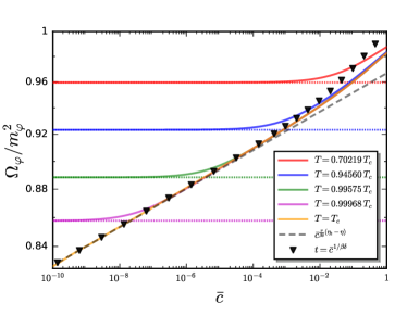
Figure 1: Ratio $\Omega_{\varphi}/m^{2}_{\varphi}$ as a function of $\bar{c}=c/c_{0}$ for various temperatures close to $T_{c}$, where $c_{0}$ denotes the value of $c$ with physical pion mass in QCD as shown in the supplement. The dotted lines correspond to values of $D_{\varphi}(T)$ in the pure SSB limit. The triangle points stands for results with a variational temperature with $t=\bar{c}^{1/{\beta\delta}}$. The gray dashed line denotes the scaling line $\sim\bar{c}^{\frac{\nu}{\beta\delta}(\eta_{t}-\eta)}$.

It is found that the prediction above from the scaling theory perfectly matches the result of the dispersion relation achieved in the fully numeric approach. In Fig. 1, we plot $\Omega_{\varphi}/m_{\varphi}^{2}$ as a function of the strength of the explicit symmetry breaking at several fixed values of temperature as well as a variational temperature with $t=\bar{c}^{1/{\beta\delta}}$ with $\bar{c}=c/c_{0}$, where $c_{0}$ denotes the value of $c$ corresponding to the physical pion mass in QCD as shown in the supplement. For $\bar{c}\ll t^{\beta\delta}$, the ratio $\Omega_{\varphi}/m^{2}_{\varphi}$ approaches to the value of $D_{\varphi}$ as $c\rightarrow 0$. On the contrary, when $\bar{c}\gtrsim t^{\beta\delta}$, the anomalous scaling regime 2 takes over, resulting in a strong breakdown of the relation 1. At the critical temperature $T=T_{c}$, the scaling regime stretches to $\bar{c}=0$, and therefore the relation 1 is not obeyed for any $c\neq 0$. In Fig. 1 we also show the scaling line $\sim\bar{c}^{\frac{\nu}{\beta\delta}(\eta_{t}-\eta)}$, where the critical exponents are computed through fixed-point equations within the fRG approach, see the supplement for their values and more details. It is found that the numerical results at $T=T_{c}$ are in excellent agreement with the scaling line when the chiral limit is approached, i.e., $c\to 0$. More importantly, one finds that a deviation between the numerical results and the scaling line takes place when $\bar{c}\gtrsim 10^{-6}\sim 10^{-4}$, corresponding to the pion mass at very low temperature $m_{\pi 0}\gtrsim 0.1\sim 1$ MeV , from which one can estimate the size of the dynamic critical region, that is $m_{\pi 0}\lesssim 0.1\sim 1$ MeV.

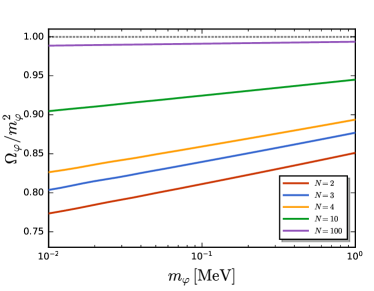
Figure 2: Ratio $\Omega_{\varphi}/m^{2}_{\varphi}$ as a function of $m_{\varphi}$ for different values of $N$ at $T=T_{c}$, where the gray dashed line denotes the value of $D_{\varphi}(T_{c})$ in the large $N$ limit.

Finally, our statement can be formulated as that the proposed relation 1 works as long as the critical fluctuations can be neglected which is always true in the hydrodynamic regime. For this reason, we shall name it ‘hydrodynamic universality’. When $T$ is sufficiently close to $T_{c}$ that the Higgs mass becomes of the same order as the pseudo-Goldstone mass, the critical slowing down has to be taken into account and the anomalous scaling behavior 2 emerges. Note that such a universality governed by the critical point is of course beyond the standard hydrodynamic regime and can be termed ‘critical universality’.

From finite N’s to the large N limit.– The O($N$) critical model can be applied to describe a wide range of interacting systems, including the Ising model ($N=1$), the XY model ($N=2$), the Heisenberg antiferromagnet ($N=3$) and the low energy QCD ($N=4$) matter, etc.

We redo the fRG calculations for different values of $N$. The relevant results of the ratio $\Omega/m_{\varphi}^{2}$ as a function of the pseudo-Goldstone mass at $T=T_{c}$ are shown in Fig. 2. The tendency is that the scaling exponent $\Delta_{\eta}$ becomes smaller for larger $N$. In the limit of large $N$, one is able to obtain analytic $\eta$ and $\eta_{t}$ which are detailed in the supplement. The anomalous dimensions both approach to zero in the way that $\{\eta,\,\eta_{t}\}\sim N^{-1}$ when $N\to\infty$. Despite that the system still experiences critical slowing down, the non-equilibrium fluctuations become negligible and $\Omega/m_{\varphi}^{2}$ becomes $c$-independent in the large $N$ limit. Moreover, we find that its value approaches to the value of $D_{\varphi}$. In this case, relation 1 is valid even beyond the standard hydrodynamic regime (as long as $c$ is small). Therefore, one should not expect that the anomalous scaling regime 2 can be observed in ‘mean-field systems’ or classical holographic models where the dynamic critical exponent is $z=2+\eta_{t}-\eta\rightarrow 2$ in the large $N$ limit. See discussions on the universality class of holographic systems in [42, 43].

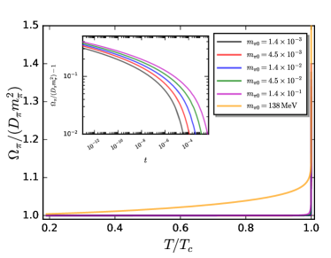
Figure 3: Ratio $\Omega_{\pi}/(D_{\pi}\,m_{\pi}^{2})$ as a function of the temperature for different values of $m_{\pi 0}$.

Damping of pions near the chiral phase transition.– The QCD matter below the critical temperature of chiral phase transition possesses a broken approximate symmetry $\text{SU(2)}_{\text{L}}\times\text{SU(2)}_{\text{R}}$ $\simeq$ O$(4)$. Then, the dynamics of pions (the associated pseudo-Goldstones in the broken phase) is often investigated via the O($4$) model. To that end, we adopt the identification that $\delta\sigma$ as the sigma meson and $\varphi\equiv\pi$ as pions.

In Fig. 3, we plot the ratio $\Omega_{\pi}/(D_{\pi}\,m_{\pi}^{2})$ as a function of the temperature for different values of the pion mass at very low temperatures $m_{\pi 0}$. Indeed, it is found that the ratio is very close to unity at all temperatures far below $T_{c}$. Its value becomes very sensitive to the value of $m_{\pi 0}$ near the critical point when $t\ll 1$. For the experiment result $m_{\pi 0}\approx 138$ MeV, we expect that the deviation from 1 becomes obvious ($\sim 10\%$) at $T\approx 0.994\,T_{c}$. When $T\to T_{c}$, we find that the deviation displays a scaling growth

$$\frac{\Omega_{\pi}}{D_{\pi}m_{\pi}^{2}}-1\propto t^{-(\eta_{t}-\eta)\nu},$$ (13)

leading to $\Omega_{\pi}\gg D_{\pi}m_{\pi}^{2}$ very close to the chiral phase transition. Note that this cannot be observed in the AdS/QCD model where the large $N$ limit is taken [18].

Conclusion and Outlook.– In this work, we investigate the real-time dynamics of pseudo-Goldstones in a relaxational O($N$) model by applying the SK formalism of the fRG, aiming to extend the scope of the study on the damping rate to the critical region. As verified in this paper, the proposed damping-diffusivity relation 1 governed by the hydrodynamic regime is always valid in the broken phase away from the critical point. While, in the vicinity of the critical point where the mass of the Higgs mode becomes comparable to the screening mass of the pseudo-Goldstone modes, $\Omega_{\varphi}/m_{\varphi}^{2}$ is no longer equal to the Goldstone diffusivity but instead displays a novel universal scaling behavior 2 controlled by the critical slowing down as well as the non-equilibrium fluctuations. Despite that this work is based on a specific model, our conclusion should be applicable to general interacting systems with spontaneously broken approximate symmetries.

Nevertheless, as we have mentioned this model is not able to describe the propagating feature of the pseudo-Goldstone modes. To make it more realistic, it is necessary to couple the order parameter $\phi_{a}$ to an almost conserved charge which generates a pair of soft modes with a finite sound speed as well as a finite pole mass. Furthermore, it should also be intriguing to verify our result using other methods which allow us to handle the critical fluctuations. For instance, one can include stochastic forces in the hydrodynamic equations following the line of [2, 44, 45, 46, 47, 48] or calculate the ‘hydrodynamic loops’ using the Schwinger-Keldysh field theory of fluctuating hydrodynamics [49, 50, 51, 52, 53, 54, 55]. Another direction is that one can enlarge the hydrodynamic description by considering the effects of Higgs mode in holographic systems near critical points [56, 57], and verify whether the damping-diffusivity relation is satisfied up to $T_{c}$ in the large $N$ limit.

Acknowledgements.– We would like to thank Matteo Baggioli, Blaise Goutéraux, Jan M. Pawlowski, Fabian Rennecke, Nicolas Wink and Hongbao Zhang for inspiring discussions and reading a previous version of this manuscript. This work is supported by the National Natural Science Foundation of China (NSFC) under Grant No.12175030, No.12147101, No.12275038 and No.12047503. W.J.L. also acknowledges the sponsorship from the Peng Huanwu Visiting Professor Program in 2023 and Institute of Theoretical Physics-Chinese Academy of Sciences for the warm hospitality during which part of this work was completed.

Supplemental Materials

The supplemental materials provide some details in sequence in line with the main text.

S.1 Setup of the relaxation model within the fRG

In the effective action in Eq. 3, the potential term on the Schwinger-Keldysh contour can be expressed as $V(\rho_{+})-V(\rho_{-})$ with

$$\rho_{\pm}\equiv\sum_{a=0}^{N-1}\frac{\phi^{2}_{a,\pm}}{2}\,,$$ (14)

corresponding to the forward and backward time evolution branch, respectively. Taking the Keldysh rotation as follows

$$\phi_{a,\pm}=\frac{1}{\sqrt{2}}\left(\phi_{a,c}\pm\phi_{a,q}\right)\,,$$ (15)

and expanding the potential in terms of $q$-fields, we have

$$V(\rho_{+})-V(\rho_{-})=V^{\prime}(\rho_{c})\,\phi_{a,q}\,\phi_{a,c}+\mathcal{O}(\phi_{a,q}^{3})\,,$$ (16)

up to the quadratic order.

From the real-time effective action in Eq. 3, one can obtain the flow equation of the effective potential within the functional renormalization group (fRG) approach, which reads

$$\partial_{\tau}u^{\prime}(\bar{\rho})= (-2+\eta)u^{\prime}(\bar{\rho})+(1+\eta)\bar{\rho}u^{(2)}(\bar{\rho})-\frac{1}{4\pi^{2}}\frac{2}{3}\left(1-\frac{\eta}{5}\right)\left[\frac{3u^{(2)}(\bar{\rho})+2\bar{\rho}u^{(3)}(\bar{\rho})}{\big{(}1+u^{\prime}(\bar{\rho})+2\bar{\rho}u^{(2)}(\bar{\rho})\big{)}^{2}}+(N-1)\frac{u^{(2)}(\bar{\rho})}{\big{(}1+u^{\prime}(\bar{\rho})\big{)}^{2}}\right]\,,$$ (17)

where we have defined the dimensionless, renormalized field and potential, viz.,

$$\bar{\rho}=Z^{(i)}_{\varphi}T^{-1}k^{-1}\rho\,,\qquad u(\bar{\rho})=T^{-1}k^{-3}V(\rho)\,,$$ (18)

with the temperature $T$ and the renormalization group (RG) scale $k$. Here we have used $\rho$ instead of $\rho_{c}$ for simplicity for the subscript of ‘classical’ field. The flow in Eq. 17 is formulated in terms of the RG time $\tau=\ln(k/\Lambda)$, where $\Lambda$ is some reference scale, e.g., an ultraviolet (UV) cutoff scale. Note that in order to arrive at the flow equation in Eq. 17 as well as those in what follows, we have used the optimized infrared (IR) regulator in fRG, see, e.g., [35] for more details.

The static and dynamic anomalous dimensions are related to the spatial and temporal wave function renormalizations through

$$\eta=-\frac{\partial_{\tau}Z^{(i)}_{\varphi}}{Z^{(i)}_{\varphi}}\,,\qquad\eta_{t}=-\frac{\partial_{\tau}Z^{(t)}_{\varphi}}{Z^{(t)}_{\varphi}}\,,$$ (19)

respectively. Within the modified local potential approximation to the effective action in Eq. 3, usually called the $\mathrm{LPA}^{\prime}$ truncation, one finds for the two anomalous dimensions

$$\eta= \frac{2}{3\pi^{2}}\frac{\bar{\rho}_{0}\big{(}u^{(2)}(\bar{\rho}_{0})\big{)}^{2}}{\big{(}1+u^{\prime}(\bar{\rho}_{0})\big{)}^{2}\big{(}1+u^{\prime}(\bar{\rho}_{0})+2\bar{\rho}_{0}u^{(2)}(\bar{\rho}_{0})\big{)}^{2}}\,,$$ (20)

$$\eta_{t}= \frac{1}{30\pi^{2}}(5-\eta)\bar{\rho}_{0}^{2}\big{(}u^{(2)}(\bar{\rho}_{0})\big{)}^{2}\big{(}1+u^{\prime}(\bar{\rho}_{0})\big{)}^{-2}\big{(}1+u^{\prime}(\bar{\rho}_{0})+2\bar{\rho}_{0}u^{(2)}(\bar{\rho}_{0})\big{)}^{-2}\big{(}1+u^{\prime}(\bar{\rho}_{0})+\bar{\rho}_{0}u^{(2)}(\bar{\rho}_{0})\big{)}^{-2}$$

$$\times\Big{[}\big{(}1+u^{\prime}(\bar{\rho}_{0})\big{)}^{2}+4\big{(}1+u^{\prime}(\bar{\rho}_{0})\big{)}\big{(}1+u^{\prime}(\bar{\rho}_{0})+2\bar{\rho}_{0}u^{(2)}(\bar{\rho}_{0})\big{)}+\big{(}1+u^{\prime}(\bar{\rho}_{0})+2\bar{\rho}_{0}u^{(2)}(\bar{\rho}_{0})\big{)}^{2}\Big{]}\,,$$ (21)

where the potential is computed on the expectation value of the field $\bar{\rho}_{0}$, which satisfies the equation of motion (EoM) as follows

$$\sqrt{2\rho_{0}}V^{\prime}(\rho_{0})-c=0\,,$$ (22)

with $\bar{\rho}_{0}=Z^{(i)}_{\varphi}T^{-1}k^{-1}\rho_{0}$. The EoM in Eq. 22 results from the effective action in Eq. 3 by differentiating with respect to the ‘quantum’ field.

Observables	Values [MeV]	Parameters
$f_{\pi}$	93.5	$\Lambda=430\,\mathrm{MeV}$
$m_{\pi}$	137.2	$\rho_{\Lambda}=3.84\times 10^{3}\,\mathrm{MeV}^{2}$
$m_{\sigma}$	567.2	$\lambda_{\Lambda}=17.5$
$f_{\pi}^{\chi}$	87.4	$c=1.76\times 10^{6}\,\mathrm{MeV}^{3}$

Table 1: Observables and parameters in the relaxational O(4) model within the functional renormalization group approach.

In our numerical calculations, the flow equation of effective potential in Eq. 17 is integrated on a grid of the potential from an UV initial value $\Lambda$ to the IR limit $k\to 0$, with the static anomalous dimension in Eq. 20 computed at each value of the RG scale. At the initial UV cutoff $k=\Lambda$, the effective potential is parameterized as

$$V^{\prime}_{k=\Lambda}(\rho)=\lambda_{\Lambda}(\rho-\rho_{\Lambda})\,.$$ (23)

Note only the derivative of potential is relevant, that is the reason why $V^{\prime}$ rather than $V$ is specified in Eq. 23. The initial UV scale $\Lambda$, the parameters $\rho_{\Lambda}$ and $\lambda_{\Lambda}$ in the potential at the initial scale, and the strength of explicit symmetry breaking $c$ as shown in the effective action in 3 constitute the set of parameters for the relaxation model within the fRG. The values of model parameters adopted in this work are collected in Tab. 1, where the observables produced at low temperature, say $T=1$ MeV, are also presented. In Tab. 1 the mass of pseudo-Goldstones, i.e., the pion mass in low energy QCD, $m_{\varphi}\equiv m_{\pi}=137.2$ MeV, is the physical mass in the real world. $m_{\sigma}$ denotes the mass of sigma mode. The pion decay constant at physical pion mass is given by $f_{\pi}=\sqrt{2\rho_{c0}}$, and $f_{\pi}^{\chi}$ stands for the pion decay constant in the chiral limit, to wit, vanishing pion mass. Moreover, within the parameters in Tab. 1 one finds for the critical temperature of phase transition in the chiral limit $T_{c}=141.633955(10)$ MeV. This precision of $T_{c}$ is necessary for the scaling analysis in this work. Note that the anomalous damping of the pseudo-Goldstone modes in the critical region found in the main text does not depend on the specific values of model parameters.

The values of critical exponents in the $\mathrm{LPA}^{\prime}$ truncation are found to be $\eta_{t}=0.054424$, $\eta=0.037320$, $\nu=0.78110$, $\beta=0.40513$, $\delta=4.7841$, which are calculated by solving the fixed-point equation, i.e., $\partial_{\tau}u^{\prime}=0$ in Eq. 17, see, e.g., [58] for more details.

S.2 The Einstein relation for Goldstone fields in the pure SSB limit

When the broken O($N$) symmetry is exact, i.e., $m_{\varphi}\to 0$, we have that $\Omega_{\varphi}\to 0$ and 6 becomes a standard diffusive dispersion with the transport coefficient

$$D_{\varphi}(T)\equiv\frac{Z_{\varphi}^{(i)}(T,c=0)}{Z_{\varphi}^{(t)}(T,c=0)}\,.$$ (24)

In this case, the physical meaning of $Z^{(t,i)}_{\varphi}(T,0)$ is manifest. From Eq. 5, we have that

$$G_{\varphi\varphi}^{R}(\omega,q)=\frac{\mathrm{i}Z^{(t)}_{\varphi}(T,0)\omega+Z^{(i)}_{\varphi}(T,0)q^{2}}{\big{(}Z^{(t)}_{\varphi}(T,0)\omega\big{)}^{2}+\big{(}Z^{(i)}_{\varphi}(T,0)q^{2}\big{)}^{2}}\,.$$ (25)

Then, $1/Z^{(t)}_{\varphi}(T,0)$ plays the role of the ‘Goldstone conductivity’ satisfying the Kubo formula for the Goldstone fields

$$\sigma_{\varphi}\equiv\frac{1}{Z^{(t)}_{\varphi}(T,0)}=\lim_{\omega\rightarrow 0}\,\omega\,\text{Im}\,G_{\varphi\varphi}^{R}(\omega,q=0)\,,$$ (26)

Note that Eq. 26 can also be recast as the standard Kubo formula for the retarded correlator of $\partial_{t}\varphi$ like in [12, 21]. Furthermore, defining $\lambda=\partial_{i}\varphi$, it is obvious to see that

$$\chi_{\lambda\lambda}\equiv\frac{1}{Z^{(i)}_{\varphi}(T,0)}=\lim_{q\rightarrow 0}q^{2}\,G_{\varphi\varphi}^{R}(0,q)\,.$$ (27)

Therefore, the inverse of the Goldstone stiffness $1/Z^{(i)}_{\varphi}(T,0)$ can be understood as the ‘Goldstone susceptibility’ [18]. Then, Eq.24 is essentially an Einstein relation for the Goldstone fields in the pure SSB pattern.

S.3 Numerical verification of Eq. 8 in the main text

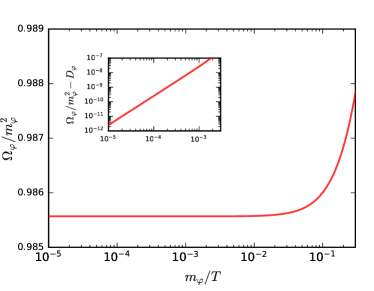
Figure 4: Ratio $\Omega_{\varphi}/m^{2}_{\varphi}$ as a function of $m_{\varphi}/T$ with $T=0.3\,T_{c}$ and $N=4$. The inset shows the subleading term of mass correction, i.e., $\Omega_{\varphi}/m_{\varphi}^{2}-D_{\varphi}$ as a function of $m_{\varphi}/T$.

In Fig. 4 we show the dependence of $\Omega_{\varphi}/m^{2}_{\varphi}$ on the mass of pseudo-Goldstones, where the temperature is chosen a value, $T=0.3\,T_{c}$ far lower than the critical temperature. The subleading term of the expansion in Eq. 8 is shown in the inlay, from which one can extract the exponent $\alpha$

$$\Omega_{\varphi}/m_{\varphi}^{2}-D_{\varphi}(T)\propto(m_{\varphi}/T)^{\alpha}\,,$$ (28)

with $\alpha=2.0056$, which is equal to 2 within errors.

S.4 Scaling behavior of the pseudo-Goldstone mass and Higgs mass

Employing the EoM of fields in Eq. 22, one arrives at the mass of the pseudo-Goldstone modes immediately as

$$m_{\varphi}^{2}=\frac{V^{\prime}(\rho_{0})}{Z^{(i)}_{\varphi}}=\frac{c}{\sigma_{0}Z^{(i)}_{\varphi}}\,,$$ (29)

where the order parameter $\sigma_{0}=\sqrt{2\rho_{0}}$ plays the role of magnetization. When the reduced temperature $t\to 0$ and in the critical region, one has $\sigma_{0}\sim c^{1/\delta}$. Moreover, one finds from the scaling function of the spatial wave function renormalization in Eq. 9 $Z^{(i)}_{\varphi}\sim c^{-\nu\eta/(\beta\delta)}$. Consequently, in the case of $t\to 0$ one is led to

$$m_{\varphi}^{2}\sim\frac{c}{c^{\frac{1}{\delta}}c^{-\frac{\nu\eta}{\beta\delta}}}=c^{\frac{2\nu}{\beta\delta}}\,,$$ (30)

which is Eq. 12 in the main text. In the last step of Eq. 30 we have used the scaling relations for different critical exponents as follows

$$\beta=\frac{\nu}{2}(d-2+\eta)\,,\qquad\delta=\frac{d+2-\eta}{d-2+\eta}\,,$$ (31)

where $d$ denotes the spatial dimension.

We proceed with the scaling analysis of the mass of sigma mode. It is very known that the sigma mass is related to the correlation length $\xi$ through $m_{\sigma}=\xi^{-1}$, and the correlation length behaves as $\xi\sim t^{-\nu}$. Thus, one finds for the scaling behavior of the sigma mass

$$m_{\sigma}^{2}=t^{2\nu}f^{\sigma}(\mathbb{z})\,,$$ (32)

with the scaling variable $\mathbb{z}=tc^{-1/(\beta\delta)}$ and the scaling function $f^{\sigma}(\mathbb{z})$. In the case of $t\to 0$, the reduced temperature in Eq. 32 has to be eliminated by the scaling function, which leaves use with

$$m_{\sigma}^{2}\sim c^{\frac{2\nu}{\beta\delta}}\,.$$ (33)

Comparing Eq. 30 and Eq. 33, we find that both the Goldstone and sigma masses have the same scaling dependence on the strength of symmetry breaking $c$ in the critical region.

S.5 Large $N$ limit

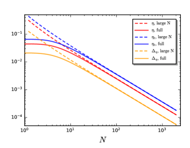
Figure 5: Dynamic anomalous dimension $\eta_{t}$, static anomalous dimension $\eta$ and their difference $\Delta_{\eta}\equiv\eta_{t}-\eta$ as functions of $N$. Here, the solid lines denote the full numeric results obtained in 17, 20 and 21, and the dashed ones denote that obtained from the expressions of large $N$ in 37.

In this section we discuss the large $N$ limit for the relaxation model in Section S.1. In the large $N$ limit, the flow of effective potential in Eq. 17 is simplified as

$$\partial_{\tau}u^{\prime}(\bar{\rho})= (-2+\eta)u^{\prime}(\bar{\rho})+(1+\eta)\bar{\rho}u^{(2)}(\bar{\rho})-\frac{1}{4\pi^{2}}\frac{2}{3}\left(1-\frac{\eta}{5}\right)(N-1)\frac{u^{(2)}(\bar{\rho})}{\big{(}1+u^{\prime}(\bar{\rho})\big{)}^{2}}\,.$$ (34)

We are interested in the fixed-point solution of the flow equation above, i.e., $\partial_{\tau}u^{\prime}_{*}(\bar{\rho})=0$. The fixed-point equation in 34 can be solved analytically through an implicit formulation, whose solution reads

$$\bar{\rho}=\frac{1}{30\pi^{2}}\frac{(5-\eta)}{1+\eta}(N-1)\,{}_{2}F_{1}\left(2,1+\frac{3}{\eta-2};\frac{2\eta-1}{\eta-2};-u^{\prime}_{*}(\bar{\rho})\right)+\mathcal{C}u^{\prime}_{*}(\bar{\rho})^{\frac{1+\eta}{2-\eta}}\,,$$ (35)

with a constant $\mathcal{C}$ to be determined, where ${}_{2}F_{1}$ is a hypergeometric function with a general notation ${}_{p}F_{q}\left(a_{1},\ldots,a_{p};b_{1},\ldots,b_{q};z\right)$. As for the last term Eq. 35, since the exponent $(1+\eta)/(2-\eta)$ is not an integer in general, which would result in a branch cut for $u^{\prime}_{*}(\bar{\rho})<0$. In consequence, the constant $\mathcal{C}$ has to be vanishing to make sure that the potential is analytic. The minimal point of the potential is determined by the EoS in Eq. 22. In the chiral limit one has $u^{\prime}_{*}(\bar{\rho}_{0})=0$, which leaves us with

$$\bar{\rho}_{0}=\frac{1}{30\pi^{2}}\frac{(5-\eta)}{(1+\eta)}(N-1)\,,\qquad u^{(2)}_{*}(\bar{\rho}_{0})=15\pi^{2}\frac{(1-2\eta)}{(5-\eta)}\frac{1}{(N-1)}\,.$$ (36)

Inserting the expressions above as well as $u^{\prime}_{*}(\bar{\rho}_{0})=0$ into Eq. 20 and Eq. 21, one obtains analytic expressions of the static and dynamic anomalous dimensions as follows

$$\eta=\frac{5}{N-1}\frac{(1+\eta)(1-2\eta)^{2}}{(5-\eta)(2-\eta)^{2}}\,,\qquad\eta_{t}=\frac{1}{9(N-1)}\frac{(1-2\eta)^{2}(13+15\eta-2\eta^{3})}{(2-\eta)^{2}}\,.$$ (37)

These are implicit functions. But one can still see clearly that $\eta\to 0$ and $\eta_{t}\to 0$ when $N\to\infty$. Then, the scaling exponent $\Delta_{\eta}\equiv\eta_{t}-\eta$ also becomes trivial in the large $N$ limit. Numerical calculations of Eq. 37 are presented in Fig. 5 in dashed lines, which are also compared with the full results obtained in 17, 20 and 21.

In the following we adopt the method of eigenperturbations to calculate the critical exponent $\nu$ in the large $N$ limit, cf. e.g., [58]. A small perturbation of the effective potential around the fixed point can be described as

$$u(\bar{\rho})=u_{*}(\bar{\rho})+\epsilon\,\mathrm{e}^{-\omega\tau}v(\bar{\rho})\,,$$ (38)

with a small parameter $\epsilon$, where $\omega$ and $v(\bar{\rho})$ stand for the eigenvalue and eigenfunction of the perturbation, respectively. Substituting Eq. 38 into Eq. 34, one is led to

$$\omega v(\bar{\rho})=3v(\bar{\rho})-(1+\eta)\bar{\rho}\,v^{\prime}(\bar{\rho})+\frac{5-\eta}{30\pi^{2}}\frac{(N-1)v^{\prime}(\bar{\rho})}{\big{(}1+u_{*}^{\prime}(\bar{\rho})\big{)}^{2}}\,.$$ (39)

This equation can be solved analytically, and its solution is given by

$$v(\bar{\rho})=\mathcal{C}_{v}\Big{[}u^{\prime}_{*}(\bar{\rho})\Big{]}^{\frac{3-\omega}{2-\eta}}\,,$$ (40)

with a constant $\mathcal{C}_{v}$. Since the Wilson-Fisher fixed point has the property $u^{\prime}_{*}(\bar{\rho}=0)<0$, in order to warrant that the eigenfunction in Eq. 40 is analytic, one has to choose the exponent there to be positive integers, i.e.,

$$\frac{3-\omega_{n}}{2-\eta}=n+1\,,\qquad n=0,1,2,\cdots\,.$$ (41)

Thus, we are led to

$$\omega_{n}=3-(n+1)(2-\eta)\,.$$ (42)

As we have show above, $\eta\to 0$ when $N\to\infty$. So, only the first eigenvalue is relevant, i.e., $\omega_{0}=1+\eta>0$. The critical exponent reads

$$\nu=\frac{1}{\omega_{0}}=\frac{1}{1+\eta}\,.$$ (43)

References

- Son and Stephanov [2002a] D. T. Son and M. A. Stephanov, Pion propagation near the QCD chiral phase transition, Phys. Rev. Lett. 88, 202302 (2002a), arXiv:hep-ph/0111100 .
- Son and Stephanov [2002b] D. T. Son and M. A. Stephanov, Real time pion propagation in finite temperature QCD, Phys. Rev. D 66, 076011 (2002b), arXiv:hep-ph/0204226 .
- Gruner [1994] G. Gruner, The dynamics of spin-density waves, Rev. Mod. Phys. 66, 1 (1994).
- Fogler and Huse [2000] M. M. Fogler and D. A. Huse, Dynamical response of a pinned two-dimensional Wigner crystal, Phys. Rev. B. 62, 7553 (2000).
- Fu et al. [2020] W.-j. Fu, J. M. Pawlowski, and F. Rennecke, QCD phase structure at finite temperature and density, Phys. Rev. D 101, 054032 (2020), arXiv:1909.02991 [hep-ph] .
- Gao and Pawlowski [2021] F. Gao and J. M. Pawlowski, Chiral phase structure and critical end point in QCD, Phys. Lett. B 820, 136584 (2021), arXiv:2010.13705 [hep-ph] .
- Dupuis et al. [2021] N. Dupuis, L. Canet, A. Eichhorn, W. Metzner, J. M. Pawlowski, M. Tissier, and N. Wschebor, The nonperturbative functional renormalization group and its applications, Phys. Rept. 910, 1 (2021), arXiv:2006.04853 [cond-mat.stat-mech] .
- Gunkel and Fischer [2021] P. J. Gunkel and C. S. Fischer, Locating the critical endpoint of QCD: Mesonic backcoupling effects, Phys. Rev. D 104, 054022 (2021), arXiv:2106.08356 [hep-ph] .
- Fu [2022] W.-j. Fu, QCD at finite temperature and density within the fRG approach: an overview, Commun. Theor. Phys. 74, 097304 (2022), arXiv:2205.00468 [hep-ph] .
- Braun et al. [2023a] J. Braun et al., Soft modes in hot QCD matter, (2023a), arXiv:2310.19853 [hep-ph] .
- Gell-Mann et al. [1968] M. Gell-Mann, R. J. Oakes, and B. Renner, Behavior of current divergences under SU(3) x SU(3), Phys. Rev. 175, 2195 (1968).
- Amoretti et al. [2019a] A. Amoretti, D. Areán, B. Goutéraux, and D. Musso, Universal relaxation in a holographic metallic density wave phase, Phys. Rev. Lett. 123, 211602 (2019a), arXiv:1812.08118 [hep-th] .
- Andrade and Krikun [2019] T. Andrade and A. Krikun, Coherent vs incoherent transport in holographic strange insulators, JHEP 05, 119, arXiv:1812.08132 [hep-th] .
- Ammon et al. [2019] M. Ammon, M. Baggioli, and A. Jiménez-Alba, A Unified Description of Translational Symmetry Breaking in Holography, JHEP 09, 124, arXiv:1904.05785 [hep-th] .
- Donos et al. [2021] A. Donos, P. Kailidis, and C. Pantelidou, Dissipation in holographic superfluids, JHEP 09, 134, arXiv:2107.03680 [hep-th] .
- Ammon et al. [2022] M. Ammon, D. Arean, M. Baggioli, S. Gray, and S. Grieninger, Pseudo-spontaneous symmetry breaking in hydrodynamics and holography, JHEP 03, 015, arXiv:2111.10305 [hep-th] .
- Zhong and Li [2022] Y.-Y. Zhong and W.-J. Li, Transverse Goldstone mode in holographic fluids with broken translations, Eur. Phys. J. C 82, 511 (2022), arXiv:2202.05437 [hep-th] .
- Cao et al. [2022] X. Cao, M. Baggioli, H. Liu, and D. Li, Pion dynamics in a soft-wall AdS-QCD model, JHEP 12, 113, arXiv:2210.09088 [hep-ph] .
- Argurio et al. [2016] R. Argurio, A. Marzolla, A. Mezzalira, and D. Musso, Analytic pseudo-Goldstone bosons, JHEP 03, 012, arXiv:1512.03750 [hep-th] .
- Amoretti et al. [2017] A. Amoretti, D. Areán, R. Argurio, D. Musso, and L. A. Pando Zayas, A holographic perspective on phonons and pseudo-phonons, JHEP 05, 051, arXiv:1611.09344 [hep-th] .
- Amoretti et al. [2019b] A. Amoretti, D. Areán, B. Goutéraux, and D. Musso, Diffusion and universal relaxation of holographic phonons, JHEP 10, 068, arXiv:1904.11445 [hep-th] .
- Baggioli [2020] M. Baggioli, Homogeneous holographic viscoelastic models and quasicrystals, Phys. Rev. Res. 2, 022022 (2020), arXiv:2001.06228 [hep-th] .
- Baggioli and Landry [2020] M. Baggioli and M. Landry, Effective Field Theory for Quasicrystals and Phasons Dynamics, SciPost Phys. 9, 062 (2020), arXiv:2008.05339 [hep-th] .
- Delacrétaz et al. [2022] L. V. Delacrétaz, B. Goutéraux, and V. Ziogas, Damping of Pseudo-Goldstone Fields, Phys. Rev. Lett. 128, 141601 (2022), arXiv:2111.13459 [hep-th] .
- Armas et al. [2023] J. Armas, A. Jain, and R. Lier, Approximate symmetries, pseudo-Goldstones, and the second law of thermodynamics, Phys. Rev. D 108, 086011 (2023), arXiv:2112.14373 [hep-th] .
- Note [1] Before that, this relation was noticed in QCD based on the argument of positivity of entropy production [44].
- Berges and Hoffmeister [2009] J. Berges and G. Hoffmeister, Nonthermal fixed points and the functional renormalization group, Nucl. Phys. B 813, 383 (2009), arXiv:0809.5208 [hep-th] .
- Gasenzer and Pawlowski [2008] T. Gasenzer and J. M. Pawlowski, Towards far-from-equilibrium quantum field dynamics: A functional renormalisation-group approach, Phys. Lett. B 670, 135 (2008), arXiv:0710.4627 [cond-mat.other] .
- Pawlowski and Strodthoff [2015] J. M. Pawlowski and N. Strodthoff, Real time correlation functions and the functional renormalization group, Phys. Rev. D 92, 094009 (2015), arXiv:1508.01160 [hep-ph] .
- Corell et al. [2021] L. Corell, A. K. Cyrol, M. Heller, and J. M. Pawlowski, Flowing with the temporal renormalization group, Phys. Rev. D 104, 025005 (2021), arXiv:1910.09369 [hep-th] .
- Huelsmann et al. [2020] S. Huelsmann, S. Schlichting, and P. Scior, Spectral functions from the real-time functional renormalization group, Phys. Rev. D 102, 096004 (2020), arXiv:2009.04194 [hep-ph] .
- Tan et al. [2022a] Y.-y. Tan, Y.-r. Chen, and W.-j. Fu, Real-time dynamics of the scalar theory within the fRG approach, SciPost Phys. 12, 026 (2022a), arXiv:2107.06482 [hep-ph] .
- Roth et al. [2022] J. V. Roth, D. Schweitzer, L. J. Sieke, and L. von Smekal, Real-time methods for spectral functions, Phys. Rev. D 105, 116017 (2022), arXiv:2112.12568 [hep-ph] .
- Braun et al. [2023b] J. Braun et al., Renormalised spectral flows, SciPost Phys. Core 6, 061 (2023b), arXiv:2206.10232 [hep-th] .
- Chen et al. [2023] Y.-r. Chen, Y.-y. Tan, and W.-j. Fu, Critical dynamics within the real-time fRG approach, (2023), arXiv:2312.05870 [hep-ph] .
- Roth and von Smekal [2023] J. V. Roth and L. von Smekal, Critical dynamics in a real-time formulation of the functional renormalization group, JHEP 10, 065, arXiv:2303.11817 [hep-ph] .
- Batini et al. [2023] L. Batini, E. Grossi, and N. Wink, Dissipation dynamics of a scalar field, Phys. Rev. D 108, 125021 (2023), arXiv:2309.06586 [hep-th] .
- Hohenberg and Halperin [1977] P. Hohenberg and B. Halperin, Theory of Dynamic Critical Phenomena, Rev. Mod. Phys. 49, 435 (1977).
- Note [2] Since the Goldstones are identical in this model, we will omit the subscript ‘’ hereafter.
- Note [3] Throughout the work, is defined as the critical temperature in the purely SSB limit, namely .
- Note [4] Here, we use an extra subscript ‘0’ to denote values of the observables at very low temperatures.
- Maeda et al. [2009] K. Maeda, M. Natsuume, and T. Okamura, Universality class of holographic superconductors, Phys. Rev. D 79, 126004 (2009), arXiv:0904.1914 [hep-th] .
- Natsuume and Okamura [2011] M. Natsuume and T. Okamura, Dynamic universality class of large-N gauge theories, Phys. Rev. D 83, 046008 (2011), arXiv:1012.0575 [hep-th] .
- Grossi et al. [2020] E. Grossi, A. Soloviev, D. Teaney, and F. Yan, Transport and hydrodynamics in the chiral limit, Phys. Rev. D 102, 014042 (2020), arXiv:2005.02885 [hep-th] .
- Grossi et al. [2021] E. Grossi, A. Soloviev, D. Teaney, and F. Yan, Soft pions and transport near the chiral critical point, Phys. Rev. D 104, 034025 (2021), arXiv:2101.10847 [nucl-th] .
- Soloviev [2022] A. Soloviev, Transport near the chiral critical point, EPJ Web Conf. 258, 05008 (2022), arXiv:2111.11375 [nucl-th] .
- Florio et al. [2022] A. Florio, E. Grossi, A. Soloviev, and D. Teaney, Dynamics of the critical point in QCD, Phys. Rev. D 105, 054512 (2022), arXiv:2111.03640 [hep-lat] .
- Florio et al. [2023] A. Florio, E. Grossi, and D. Teaney, Dynamics of the critical point in QCD: critical pions and diffusion in Model G, (2023), arXiv:2306.06887 [hep-lat] .
- Crossley et al. [2017] M. Crossley, P. Glorioso, and H. Liu, Effective field theory of dissipative fluids, JHEP 09, 095, arXiv:1511.03646 [hep-th] .
- Haehl et al. [2016] F. M. Haehl, R. Loganayagam, and M. Rangamani, Topological sigma models & dissipative hydrodynamics, JHEP 04, 039, arXiv:1511.07809 [hep-th] .
- Liu and Glorioso [2018] H. Liu and P. Glorioso, Lectures on non-equilibrium effective field theories and fluctuating hydrodynamics, PoS TASI2017, 008 (2018), arXiv:1805.09331 [hep-th] .
- Chen-Lin et al. [2019] X. Chen-Lin, L. V. Delacrétaz, and S. A. Hartnoll, Theory of diffusive fluctuations, Phys. Rev. Lett. 122, 091602 (2019), arXiv:1811.12540 [hep-th] .
- Jain and Kovtun [2022] A. Jain and P. Kovtun, Late Time Correlations in Hydrodynamics: Beyond Constitutive Relations, Phys. Rev. Lett. 128, 071601 (2022), arXiv:2009.01356 [hep-th] .
- Jain et al. [2021] A. Jain, P. Kovtun, A. Ritz, and A. Shukla, Hydrodynamic effective field theory and the analyticity of hydrostatic correlators, JHEP 02, 200, arXiv:2011.03691 [hep-th] .
- Donos and Kailidis [2024] A. Donos and P. Kailidis, Nearly critical superfluids in Keldysh-Schwinger formalism, JHEP 01, 110, arXiv:2304.06008 [hep-th] .
- Donos and Pantelidou [2022] A. Donos and C. Pantelidou, Higgs/amplitude mode dynamics from holography, JHEP 08, 246, arXiv:2205.06294 [hep-th] .
- Donos and Kailidis [2022] A. Donos and P. Kailidis, Nearly critical holographic superfluids, JHEP 12, 028, [Erratum: JHEP 07, 232 (2023)], arXiv:2210.06513 [hep-th] .
- Tan et al. [2022b] Y.-y. Tan, C. Huang, Y.-r. Chen, and W.-j. Fu, Criticality of the universality via global solutions to nonperturbative fixed-point equations, (2022b), arXiv:2211.10249 [hep-ph] .