Reducing the runtime of fault-tolerant quantum simulations in chemistry through symmetry-compressed double factorization

Abstract

Quantum phase estimation based on qubitization is the state-of-the-art fault-tolerant quantum algorithm for computing ground-state energies in chemical applications. In this context, the 1-norm of the Hamiltonian plays a fundamental role in determining the total number of required iterations and also the overall computational cost. In this work, we introduce the symmetry-compressed double factorization (SCDF) approach, which combines a compressed double factorization of the Hamiltonian with the symmetry shift technique, significantly reducing the 1-norm value. The effectiveness of this approach is demonstrated numerically by considering various benchmark systems, including the FeMoco molecule, cytochrome P450, and hydrogen chains of different sizes. To compare the efficiency of SCDF to other methods in absolute terms, we estimate Toffoli gate requirements, which dominate the execution time on fault-tolerant quantum computers. For the systems considered here, SCDF leads to a sizeable reduction of the Toffoli gate count in comparison to other variants of double factorization or even tensor hypercontraction, which is usually regarded as the most efficient approach for qubitization.

1 Introduction

Quantum chemistry simulations hold a significant potential to advance many industry-relevant applications, including the development of new drugs ¹, catalysts ², and materials ³. The simulation of chemical systems from first principles requires the solution of the Schrödinger equation, a task particularly challenging for classical approaches because of the exponential growth of the computational cost with system size. Quantum computing provides a promising solution to address this scalability issue, with significant ongoing efforts focused on developing resource-efficient algorithms ⁴. Much of this work has been dedicated to approaches tailored for early-stage noisy quantum devices, such as the variational quantum eigensolver (VQE) ^{5, 6}. Besides the challenges of working with noisy hardware, optimizing the parameters in the VQE ansatz is non-trivial, and the number of required measurements grows rapidly with the system size.

The significant challenges to achieving a quantum advantage in near-term noisy devices motivate current efforts to transition towards fault-tolerant quantum computing (FTQC). Early hardware demonstrations of error-corrected logical qubits have already been achieved ^{7, 8} and many companies, including IBM ⁹ and Google ¹⁰, have announced roadmaps to build fault-tolerant quantum computers in the next few years. At the same time, a parallel effort is underway to develop quantum algorithms that can efficiently exploit error-corrected qubits.

Quantum phase estimation (QPE) can be considered as the prototypical algorithm for chemistry simulations within the FTQC framework ^{11, 12}. Within the standard formulation of QPE, the calculation of the ground state energy of a given chemical system relies on the implementation of the Hamiltonian evolution operator $\mathcal{U}[\hat{H}]=e^{-i\hat{H}\tau}$ for some duration $\tau$; this operator can be approximated in practice using the Trotter-Suzuki ¹³ formula or Taylor series expansion ¹⁴. More recently, an alternative approach for QPE has been proposed based on the quantum walk operator $\mathcal{W}[\hat{H}]=e^{-i\arccos(\hat{H}/\lambda)}$ ^{15, 16, 17}. Instead of directly returning the ground state energy, the algorithm outputs the arccosine of the ground state energy. The advantage of this procedure is that the quantum circuit corresponding to the quantum walk operator can be implemented exactly using qubitization ¹⁸. The parameter $\lambda$ in the definition of $\mathcal{W}[\hat{H}]$ corresponds to the 1-norm of the Hamiltonian, and its value is influenced by the specific representation of $\hat{H}$ and the strategy used to block encode it. This parameter plays a crucial role in the QPE efficiency, and its optimization is one of the main topics of this work.

Within the qubitization-based QPE approach, the total number of Toffoli gates scales as $\mathcal{O}\left(\frac{\lambda}{\epsilon}C_{\mathcal{W}[\hat{H}]}\right)$. Here, $\epsilon$ represents the accuracy required for the ground state energy (typically, this should be within the chemical accuracy threshold of 1.6 mHa), and the ratio $\lambda/\epsilon$ determines the total number of iterations; $C_{\mathcal{W}[\hat{H}]}$ is the Toffoli gate cost per iteration and depends on the specific approach used for implementing $\mathcal{W}[\hat{H}]$. Implementing Toffoli gates or, similarly, T gates on quantum hardware requires a procedure known as magic state distillation ^{19, 20, 17}. This process demands a considerably large number of qubits and takes significantly more time than other operations in the computation. For this reason, a reduction in the overall Toffoli gate count for a quantum algorithm is expected to lead to an equivalent reduction in the overall runtime.

While the 1-norm plays a fundamental role in determining the total number of iterations, $C_{\mathcal{W}[\hat{H}]}$ also has a significant contribution to the overall computational cost. Specifically, the computational complexity of realizing $\mathcal{W}[\hat{H}]$ depends on $\Gamma$, the amount of information needed to specify the Hamiltonian, and the specific approach employed for the quantum implementation. As discussed in Ref. 21, the combination of tensor factorizations with techniques such as unary iteration ¹⁷ and optimized QROM assisted by ancillae ^{22, 23} leads to a $\mathcal{O}(\sqrt{\Gamma})$ Toffoli gate and logical qubits scaling. Further details on the origin of this square root dependence will be provided in Sec. 3.1. A summary of the computational complexity of state-of-the-art approaches for qubitization-based QPE is presented in Table 1. Beyond a different cost in the $\mathcal{W}[\hat{H}]$ implementation, these approaches also involve different definitions of the 1-norm $\lambda$, whose scaling varies between $\mathcal{O}(N)$ and $\mathcal{O}(N^{3})$, in which $N$ is the number of spatial orbitals the Hamiltonian is expressed in.

Approach	Logical qubits	Toffoli gates
Sparse method 23	$\mathcal{O}(N+\sqrt{S})$	$\mathcal{O}((N+\sqrt{S})\lambda_{V}/\epsilon)$
Single factorization 23	$\mathcal{O}(N^{3/2})$	$\mathcal{O}(N^{3/2}\lambda_{SF}/\epsilon)$
Explicit double factorization24	$\mathcal{O}(N\sqrt{\Xi})$	$\mathcal{O}(N\lambda_{\textrm{DF}}\sqrt{\Xi}/\epsilon)$
Tensor hypercontraction21	$\mathcal{O}(N)$	$\mathcal{O}(N\lambda_{\textrm{THC}}/\epsilon)$

Table 1: Asymptotic scaling of the computational resources required by different approaches used in qubitization-based quantum phase estimation. The definition of the 1-norm $\lambda$ depends on the specific implementation. The ratio of $\lambda$ to the required precision $\epsilon$ in the final result determines the total number of iterations. $N$ denotes the number of spin orbitals, $S$ the sparsity of the Hamiltonian, and $\Xi$ the average rank of the second factorization.

A straightforward implementation based on the electronic Hamiltonian in second quantization involves $\mathcal{O}(N^{4})$ terms. To improve over this complexity, a sparse method was introduced that truncates the components of the two-electron tensor according to a chosen threshold ²³. The main limitation of this approach is that the number of remaining terms $S$ in the Hamiltonian cannot be systematically predicted, and in some cases, still behaves as $\mathcal{O}(N^{4})$. The single factorization (SF) approach applies an eigendecomposition to the two-electron tensor (see Eq. 16 below) and this effectively decreases the number of terms in the Hamiltonian to $\mathcal{O}(N^{3})$ ²³. The explicit double factorization (XDF) approach introduces a second factorization on top of the SF (see Eq. 17 below) ^{25, 26, 23, 27}. This reduces the Hamiltonian to $\mathcal{O}(N^{2}\Xi)$ pieces of information, where $\Xi$ is the average rank of the second tensor factorization. The numerical experiments for hydrogen chain considered in Sec. 3.4 show that $\Xi$ itself is characterized by a $\mathcal{O}(N)$ behavior. As discussed in Sec. 2.2, an alternative approach known as compressed double factorization (CDF) builds the tensors in the factorization by optimizing a suitable cost function ^{28, 29, 30}. The new methodology presented in this paper will be based on a variant of the CDF approach. The recent work of von Burg et al. ²⁴ has introduced an efficient quantum algorithm to implement the double-factorized Hamiltonian in the QPE framework by employing Givens rotations and qubitization ²⁴. Compared to a straightforward qubitization of the double-factorized Hamiltonian, this formulation also benefits from significantly reducing the 1-norm.

The tensor hypercontraction (THC) approach decomposes the two-electron tensor in the Hamiltonian as $g_{pqrs}\approx\sum_{\mu,\nu=1}^{N_{\textrm{THC}}}\chi_{p}^{(\mu)}\chi_{q}^{(\mu)}\zeta_{\mu\nu}\chi_{p}^{(\nu)}\chi_{q}^{(\nu)}$, where $\chi_{p}^{\mu}$ and $\zeta_{\mu\nu}$ denote the components of the tensors used for this decomposition, $N_{\textrm{THC}}$ is the THC rank, and $p$, $q$, $r$, and $s$ are indices identifying the spatial orbitals ^{31, 32}. The tensors are obtained by minimizing a cost function that determines the deviation of the decomposition from the exact two-electron tensor. The application of this approach in the context of QPE was first proposed in Ref. 21. To effectively decrease the 1-norm, the $\chi$ tensors were used as basis set rotations, applying them to redefine the representation of the corresponding creation and annihilation operators in the second-quantized Hamiltonian. In practice, this amounts to reformulating the Hamiltonian in a larger non-orthogonal basis set and new techniques were developed to block encode and qubitize it ²¹. Beyond decreasing the 1-norm, the THC approach provides a very compact representation of the Hamiltonian, with $\Gamma=\mathcal{O}(N^{2})$ and, correspondingly, an improved asymptotic computational complexity. Since this method has systemically provided the most favorable resource estimations for many examples of electronic Hamiltonians ^{21, 33}, it will serve as the main benchmark for the methodological developments proposed in this work.

This work is largely focused on the reduction of the 1-norm that has a strong impact on the number of iterations and, accordingly, on the total runtime of the QPE algorithm. Different approaches have been proposed in the literature to optimize the 1-norm. The XDF in the implementation of von Burg et al.²⁴ and the THC ²¹ benefit themselves from formulations that significantly reduce the 1-norm as compared to a straightforward transformation of the electronic Hamiltonian into Pauli words. The optimization of the 1-norm for quantum simulations has been considered in previous work. Orbital transformations were proven to improve the 1-norm values significantly ³⁴. In Ref. 35, several different approaches (including orbital transformation) were compared by considering small molecules in the minimal STO-3G basis set; it was shown that double factorization coupled with a symmetry shift provides the best results in terms of 1-norm reduction and scaling with the system size. This symmetry shift approach, described in detail in Sec. 2.3, effectively decreases the 1-norm by subtracting a function of the number operator of electrons from the electronic Hamiltonian. Since the number operator of electrons commutes with the Hamiltonian, the eigenvectors of the Hamiltonian are not affected by this shift, and the correct ground state energy can be obtained by applying a simple a posteriori correction.

The new symmetry-compressed double factorization (SCDF) approach introduced here exploits the symmetry shift idea but additionally optimizes the DF tensor decomposition to further decrease the 1-norm. Numerical demonstrations of this method include active space models of the FeMoco molecule and cytochrome P450, and hydrogen chains with up to 80 atoms. For all of these systems, SCDF, to the best of our knowledge, provides the smallest values of the 1-norm reported in the literature. This leads to a Toffoli gate count and runtime that are sizeably reduced with respect to THC (for example by one half for FeMoco and P450). The SCDF factorization has the same structure of XDF and can be implemented using the techniques proposed by von Burg et al. ²⁴. Accordingly, SCDF inherits an analogous computational complexity both in terms of Toffoli gate and logical qubit requirements (see Table 1) but with a 1-norm that scales more favorably with the number of orbitals compared to XDF (see Sec. 3.4). Despite a slightly worse asymptotic behavior than THC, the numerical applications considered in this work show that SCDF provides more systematic accuracy for ground state energies owing to a simpler numerical optimization scheme. This feature is crucial to address systems of large size and to obtain reliable properties in the thermodynamic limit.

2 Methodological approach

2.1 General double factorization framework

Within the second quantization formalism, the electronic Hamiltonian is expressed as

$$\hat{H}=E_{\textrm{nuc}}+\sum_{p,q=1}^{N}k_{pq}\hat{E}_{pq}+\frac{1}{2}\sum_{p,q,r,s=1}^{N}g_{pqrs}\hat{E}_{pq}\hat{E}_{rs},$$ (1)

where $p$, $q$, $r$, and $s$ are indices identifying the $N$ spatial orbitals, and the singlet spin-summed one-particle substitution operators are defined as $\hat{E}_{pq}\equiv\hat{a}^{{\dagger}}_{p}\hat{a}_{q}+\hat{a}^{{\dagger}}_{\bar{p}}\hat{a}_{\bar{q}}$. In this definition $\hat{a}^{{\dagger}}$ and $\hat{a}$ denote creation and annihilation operators, respectively, and the bar on top of the orbital indexes indicates a $\downarrow$ spin orbital.

In Eq. 1 the constant term $E_{\textrm{nuc}}$ corresponds to the nuclear repulsion energy,

$$g_{pqrs}=(pq|rs)=\iint d\mathbf{r}_{1}\ d\mathbf{r}_{2}\ \phi_{p}(\mathbf{r}_{1})\phi_{q}(\mathbf{r}_{1})\frac{1}{r_{12}}\phi_{r}(\mathbf{r}_{2})\phi_{s}(\mathbf{r}_{2})$$ (2)

is the two-electron tensor, and the modified one-electron tensor $k_{pq}=h_{pq}-\frac{1}{2}\sum_{r=1}^{N}g_{prrq}$ is defined in terms of the one-electron integrals

$$h_{pq}=(p|h|q)=\int d\mathbf{r}\ \phi_{p}(\mathbf{r})\left(-\frac{1}{2}\nabla^{2}-\sum_{I}\frac{Z_{I}}{r_{I}}\right)\phi_{q}(\mathbf{r}),$$ (3)

that include the kinetic and electron-nucleus interaction energies. Without loss of generality for molecular systems, the spatial orbitals $\phi(\mathbf{r})$ have been chosen to be real.

The second quantized Hamiltonian can then be expressed in a quantum computing amenable form by expanding it in terms of Pauli words using, for example, the Jordan-Wigner or Bravyi-Kitaev transformations ^{36, 37, 38}. These approaches lead to $\mathcal{O}(N^{4})$ number of terms in the Hamiltonian. Despite the polynomial growth, this number of terms poses practical challenges for noisy near-term and fault-tolerant algorithms, and, in this context, the double factorization of the Hamiltonian can provide several advantages.

The main idea of double factorization consists in decomposing the two-electron tensor in the following way ^{39, 25, 26, 23, 40, 27, 28}:

$$(pq|rs)\approx\sum_{t=1}^{N_{\textrm{DF}}}\sum_{k,l=1}^{N}U^{t}_{pk}U^{t}_{qk}V^{t}_{kl}U^{t}_{rl}U^{t}_{sl},$$ (4)

where the $\mathbf{U}^{t}$ tensors are orthonormal, namely

$$\sum_{k=1}^{N}U^{t}_{pk}U^{t}_{qk}=\delta_{pq},\quad\quad\sum_{k=1}^{N}U^{t}_{kp}U^{t}_{kq}=\delta_{pq},$$ (5)

and the “core” tensors

$$V^{t}_{kl}=V^{t}_{lk}$$ (6)

are symmetric for all $t$’s. The sum over $t$ in Eq. 4 runs up to a maximum value $N_{\textrm{DF}}$ that depends on the specific approach used to build the tensor factorization and crucially determines the trade-off between the accuracy and efficiency of the method. Depending on the specific DF implementation, the sums over $k$ and $l$ can also be limited to values $\Xi^{(t)}\leq N$. The truncation of the tensors within the double factorization approach will be further discussed below.

By inserting the factorized tensors of Eq. 4 into Eq. 1, it is possible to reformulate the second quantized Hamiltonian in terms of the operators $\tilde{a}_{kt}^{{\dagger}}=\sum_{p=1}^{N}U^{t}_{pk}\hat{a}_{p}^{{\dagger}}$ and $\tilde{a}_{kt}=\sum_{q=1}^{N}U^{t}_{qk}\hat{a}_{q}$, that create and annihilate electrons, respectively, in a new set of rotated orbitals. In order to apply these operators, it is convenient to introduce the $\hat{G}_{t}$ operators, that rotate the quantum state in the new orbital basis and, using the Thouless theorem ⁴¹, can be expressed as

$$\hat{G}^{{\dagger}}_{t}=\exp\left(\sum_{p,q=1}^{N}[\log\mathbf{U}^{t}]_{pq}\hat{a}^{{\dagger}}_{p}\hat{a}_{q}\right).$$ (7)

These rotations can be formulated in terms of Givens rotations networks that can be efficiently implemented on quantum hardware ²⁶. Within the double-factorized formalism, the Hamiltonian in second quantization can then be expressed as

$$\hat{H}=E_{\textrm{nuc}}+\sum_{p,q=1}^{N}k_{pq}\hat{E}_{pq}+\frac{1}{2}\sum_{t=1}^{N_{\textrm{DF}}}\sum_{k,l=1}^{N}V^{t}_{kl}\hat{G}_{t}^{{\dagger}}\hat{E}_{kk}\hat{E}_{ll}\hat{G}_{t}.$$ (8)

We can now apply a fermion-to-qubit mapping based on the Jordan-Wigner transformation ³⁶. Since within this framework $\hat{E}_{kk}=\hat{I}-\frac{1}{2}(\hat{Z}_{k}+\hat{Z}_{\bar{k}})$ and

$$\hat{E}_{kk}\hat{E}_{ll}=-\hat{I}+\hat{E}_{kk}+\hat{E}_{ll}+\frac{1}{4}(\hat{Z}_{k}+\hat{Z}_{\bar{k}})(\hat{Z}_{l}+\hat{Z}_{\bar{l}}),$$ (9)

the Hamiltonian can be finally expressed as:

$$\hat{H}=\!\!\!\!\!\!\! \mathcal{E}-\frac{1}{2}\sum_{k=1}^{N}f^{\text{\o}}_{k}\hat{G}_{\text{\o}}^{{\dagger}}(\hat{Z}_{k}+\hat{Z}_{\bar{k}})\hat{G}_{\text{\o}}$$ (10)

$$+\frac{1}{8}\sum_{t=1}^{N_{\textrm{DF}}}\sum_{k,l=1}^{N}V^{t}_{kl}\hat{G}_{t}^{{\dagger}}\left(\hat{Z}_{k}\hat{Z}_{l}-\delta_{kl}+\hat{Z}_{k}\hat{Z}_{\bar{l}}+\hat{Z}_{\bar{k}}\hat{Z}_{l}+\hat{Z}_{\bar{k}}\hat{Z}_{\bar{l}}-\delta_{\bar{k}\bar{l}}\right)\hat{G}_{t}.$$

In this equation, the one-electron tensor has been redefined as $f_{qp}=k_{qp}+\sum_{r=1}^{N}g_{pqrr}$ and a “single factorized” (eigenvalue) decomposition has been applied to obtain

$$f_{pq}=\sum_{k=1}^{N}U^{\text{\o}}_{pk}f^{\text{\o}}_{k}U^{\text{\o}}_{qk}.$$ (11)

The constant term $\mathcal{E}$ contains $E_{\textrm{nuc}}$ and additional constant terms originating from the one and two-body operators.

The block encoding of the double-factorized Hamiltonian can be obtained by straightforward application of the linear combination of unitaries (LCU) approach to the Hamiltonian in the form of Eq. 10 ^{42, 18}. In this case, the 1-norm takes the following value:

$$\lambda^{\textrm{LCU}}_{\textrm{DF}}=\sum_{k=1}^{N}|f^{\text{\o}}_{k}|+\frac{1}{2}\sum_{t=1}^{N_{\textrm{DF}}}\sum_{k,l=1}^{N}|V^{t}_{kl}|-\frac{1}{4}\sum_{t=1}^{N_{\textrm{DF}}}\sum_{k=1}^{N}|V^{t}_{kk}|.$$ (12)

An alternative method to block encode the double-factorized Hamiltonian has been introduced by von Burg et al. ²⁴. To introduce this approach we assume that the $\mathbf{V}^{t}$ tensors have rank one and are positive definite for every value of $t$. As discussed in the next Section, not all the approaches to build the double factorization satisfy these properties and this has important repercussions on the efficiency of a specific method. A positive-definite rank-one $\mathbf{V}^{t}$ can always be decomposed as

$$V^{t}_{kl}=W_{k}^{t}W_{l}^{t};$$ (13)

by replacing this factorization in Eq. 8 and reapplying the Jordan-Wigner transformation of the Hamiltonian takes the form

$$\hat{H}=\!\!\!\!\!\!\! \mathcal{E}-\frac{1}{2}\sum_{k=1}^{N}f^{\text{\o}}_{k}\hat{G}_{\text{\o}}^{{\dagger}}(\hat{Z}_{k}+\hat{Z}_{\bar{k}})\hat{G}_{\text{\o}}$$ (14)

$$+\frac{1}{8}\sum_{t=1}^{N_{\textrm{DF}}}\hat{G}_{t}^{{\dagger}}\left(\sum_{k=1}^{\Xi^{(t)}}W^{t}_{k}(\hat{Z}_{k}+\hat{Z}_{\bar{k}})\right)^{2}\hat{G}_{t},$$

where the sums over $k$ have been truncated at $\Xi^{(t)}\leq N$ by eliminating the elements of the $\mathbf{W}^{t}$ tensors below a certain threshold $\delta_{\textrm{DF}}$; $\Xi$, which denotes the average of the $\Xi^{(t)}$ values, has been used in the Introduction to discuss the computational complexity of double factorization (see Table 1). For this formulation of the electronic Hamiltonian we have $\Gamma=\mathcal{O}(N^{2}\Xi)$, since in the two-body term we have a sum over $N_{\textrm{DF}}$ (which is itself $\mathcal{O}(N)$), a sum over $\Xi$, and $N$ additional degrees of freedom in the basis rotations. Within this formulation, the 1-norm of the Hamiltonian is given by

$$\lambda^{\textrm{Burg}}_{\textrm{DF}}=\sum_{k=1}^{N}|f^{\text{\o}}_{k}|+\frac{1}{4}\sum_{t=1}^{N_{\textrm{DF}}}\left(\sum_{k=1}^{\Xi^{(t)}}|W^{t}_{k}|\right)^{2}.$$ (15)

This approach has two main advantages: (1) The Hamiltonian in Eq. 14 can be efficiently implemented using qubitization ¹⁸; (2) the 1-norm in Eq. 15 is typically significantly smaller with respect to the LCU 1-norm in Eq. 12. As discussed in the following Sections of the paper, the implementation of von Burg et al. benefits significantly from the low rank of the $\mathbf{V}^{t}$ tensor, and this will be an important feature included in our new SCDF methodology.

2.2 Explicit and compressed double factorization

In the previous Section, we introduced the general double factorization formalism and presented the benefits of this approach. Here, we explain the main practical schemes that can be used to build the tensor factorization in Eq. 4. These approaches fall into two main categories: (1) explicit double factorization (XDF), which builds the $\mathbf{V}^{t}$ and $\mathbf{U}^{t}$ tensors using a two-step eigenvalue or Cholesky decomposition ^{25, 26, 23, 27}; (2) compressed double factorization (CDF) and its variants that build those tensors optimizing a cost function ^{28, 29}.

Within the framework of XDF, the two-electron tensor is first decomposed in terms of eigenvalues and eigenvectors:

$$(pq|rs)=\sum_{t=1}^{N_{\textrm{DF}}}V_{pq}^{t}\lambda_{t}V_{rs}^{t}=\sum_{t=1}^{N_{\textrm{DF}}}L_{pq}^{t}L_{rs}^{t}$$ (16)

where we introduced the definition $L_{rs}^{t}\equiv\sqrt{\lambda_{t}}V_{rs}^{t}$. A second factorization can then be obtained from the eigendecomposition of the $\mathbf{L}^{t}$ tensors:

$$L_{rs}^{t}=\sum_{k=1}^{\Xi^{(t)}}U_{rk}^{t}W^{t}_{k}U_{sk}^{t},$$ (17)

whose rank has been truncated to a $t$-dependent value $\Xi^{(t)}$, which is at most equal to $N$. The combination of these two equations provides a tensor decomposition in the form of Eq. 4 by defining

$$V^{t}_{kl}\equiv W^{t}_{k}W^{t}_{l},$$ (18)

which is clearly consistent with the general definition in Eq. 13. According to Eq. 18 the $\mathbf{V}^{t}$ tensor has rank 1 and, as already mentioned in the previous Section, this is an important feature to implement efficiently the double factorized Hamiltonian using the approach of von Burg et al. ²⁴. This XDF procedure is, in principle, exact if no truncation is applied, namely $N_{\textrm{DF}}=N^{2}$ and $\Xi^{(t)}=N$. In practice, it is well known from widely used techniques such as density fitting or Cholesky decomposition^{43, 44, 45, 46} that the rank of the two-electron integrals to achieve reasonable accuracy is much smaller than $N^{2}$ and in practice $N_{\textrm{DF}}$ scales as $\mathcal{O}(N)$. Concerning the truncation of the second factorization, while the average rank $\Xi$ can be smaller than $N$ its complexity still behaves as $\mathcal{O}(N)$.

To further improve the scaling or at least the numerical complexity prefactor of the DF, it is alternatively possible to build the Hamiltonian from $\mathbf{V}^{t}$ and $\mathbf{U}^{t}$ tensors obtained by minimizing a suitable cost function. While $\mathbf{U}^{t}$ and $\mathbf{V}^{t}$ are constrained to still be orthogonal and symmetric, respectively, this type of approach takes advantage of the full rank of these tensors. This is the main idea at the base of compressed double factorization (CDF), which determines the DF tensors by minimizing the cost function ²⁸

$$\mathcal{L}^{\textrm{CDF}}(\mathbf{U}^{t},\mathbf{V}^{t})=\frac{1}{2}\left|(pq|rs)-\sum_{t=1}^{N_{\textrm{DF}}}\sum_{k,l=1}^{N}U^{t}_{pk}U^{t}_{qk}V^{t}_{kl}U^{t}_{rl}U^{t}_{sl}\right|^{2}_{\mathcal{F}},$$ (19)

where $\mathcal{F}$ denotes the Frobenius norm. With respect to XDF, a smaller value of $N_{\textrm{DF}}$ can typically achieve the same level of accuracy in the final result. Minimization of the cost function can be achieved more efficiently by alternating the optimization of the $\mathbf{V}^{t}$ and $\mathbf{U}^{t}$ tensors. The optimization with respect to $\mathbf{V}^{t}$ can be recast in the form of a linear system and solved with standard linear algebra libraries. The orthogonality of the $\mathbf{U}^{t}$ tensors should be constrained during the optimization. As explained in Appendix A, this problem can be reformulated in an unconstrained form by introducing antisymmetric orbital rotation generators. The derivatives of the cost function with respect to the components of the generators can be evaluated analytically and, since the minimization problem is non-linear in this case, a numerical unconstrained continuous optimizer such as limited-memory Broyden–Fletcher–Goldfarb–Shanno algorithm (L-BFGS) is used.

The CDF approach provides a more compact representation in terms of the $N_{\textrm{DF}}$ rank required for a given level of accuracy but usually converges to tensors $\mathbf{V}^{t}$ with large components, which in turn leads to 1-norms comparable or even larger with respect to XDF. For this purpose, a regularized compressed double factorization (RCDF) has been recently introduced that is based on the following cost function ^{29, 33}:

$$\mathcal{L}^{\textrm{RCDF}}(\mathbf{U}^{t},\mathbf{V}^{t})=\frac{1}{2}\left|(pq|rs)-\sum_{t=1}^{N_{\textrm{DF}}}\sum_{k,l=1}^{N}U^{t}_{pk}U^{t}_{qk}V^{t}_{kl}U^{t}_{rl}U^{t}_{sl}\right|^{2}_{\mathcal{F}}+\sum_{t=1}^{N_{\textrm{DF}}}\sum_{k,l=1}^{N}\rho_{tkl}|V^{t}_{kl}|^{\gamma},$$ (20)

where the components of the tensor $\rho_{tkl}$ are usually fixed to a constant value and $\gamma$ takes the values 1 or 2 for L1 and L2 regularization, respectively. The last term in the cost function can be considered as a penalty function that prevents the elements of the $\mathbf{V}^{t}$ tensor from becoming too large and, accordingly, limits the growth of the 1-norm. In Ref. 29 all numerical applications were based on the L2 regularization and this approach showed a sizeable decrease of the $\lambda^{\textrm{Burg}}_{\textrm{DF}}$ norm with respect to XDF and THC.

It is important to notice that in both the CDF and RCDF approaches, the $\mathbf{V}^{t}$ tensors are not necessarily positive definite, and their rank is unconstrained during the optimization. As discussed in Ref.  29, to generalize the approach of von Burg et al. to the (R)CDF case, it is possible to introduce the factorization

$$V^{t}_{kl}=\sum_{i=1}^{N}W_{ki}^{t}W_{li}^{t}.$$ (21)

However, this approach has two major disadvantages. First, the components of $\mathbf{W}^{t}$ are complex, requiring some modifications of the original implementation of double factorization based on qubitization. Second, with respect to Eq. 13, the tensor decomposition in Eq. 21 involves an additional sum over $N$ terms. This implies that the amount of information $\Gamma$ defining the Hamiltonian has complexity $\mathcal{O}(N^{4})$, which is of the same order as the unfactorized Hamiltonian and strongly affects the computational resource requirements. Using the RCDF tensor factorization provided in Ref. 29, in Sec. 3.3, we will show how Toffoli gate and logical qubit requirements are affected in practice for the case of cytochrome P450. Since our new SCDF method is based on a cost function analogous to those used in CDF and RCDF, this issue is overcome by constraining the $\mathbf{V}^{t}$ tensor to be rank 1 during the optimization.

2.3 Symmetry shift approach

The main idea of symmetry shift involves replacing the Hamiltonian $\hat{H}$ with $\hat{H}-\hat{S}(\mathbf{a})$, where $\hat{S}(\mathbf{a})$ is a generic symmetry operator that satisfies $[\hat{H},\hat{S}(\mathbf{a})]=0$ ^{35, 47}. The set of parameters $\mathbf{a}$ is chosen to minimize the 1-norm. Since the symmetry operator commutes with the full electronic Hamiltonian, $\hat{H}-\hat{S}(\mathbf{a})$ has the same eigenstates of $\hat{H}$ and can be directly used in QPE, taking advantage of the smaller 1-norm. The generic operator $\hat{S}(\mathbf{a})$ can be built as a function of one or multiple reciprocally commuting basic symmetry operators of which we know the eigenvalue for the ground state ahead of time. The possible choices of these symmetry operators include the number operator of electrons $\hat{N}_{e}=\sum_{k=1}^{N}\hat{E}_{kk}$, the z-projection of the spin, the total spin, and the molecular point group symmetries. The original work of Loaiza and Izmaylov ^{35, 47} focused on the $\hat{N}_{e}$ shift, which was shown to be effective to significantly reduce the 1-norm. In practice, this method is based on the shifted Hamiltonian

$$\hat{H}_{S}=\hat{H}-\hat{S}(\mathbf{a})=\hat{H}-a_{1}\hat{N}_{e}-a_{2}\hat{N}_{e}^{2},$$ (22)

where the two terms corresponding to $\hat{N}_{e}$ and $\hat{N}_{e}^{2}$ are intended to decrease the 1-norm of the one and two-body components of the Hamiltonian, respectively. The strategy to optimize the parameters $\mathbf{a}$ is detailed in Ref. 35. For the one-body term of the Hamiltonian $\hat{H}_{1}$ we have

$$\hat{H}_{1}-a_{1}\hat{N}_{e} = -\frac{1}{2}\sum_{k=1}^{N}(f_{k}^{\text{\o}}+2a_{1})\hat{G}_{\text{\o}}^{{\dagger}}\hat{E}_{kk}\hat{G}_{\text{\o}}$$ (23)

$$= -\frac{1}{2}\sum_{k=1}^{N}(f_{k}^{\text{\o}}-a_{1}^{\prime})\hat{G}_{\text{\o}}^{{\dagger}}\hat{E}_{kk}\hat{G}_{\text{\o}},$$

where we have used the fact that $\hat{N}_{e}$ commutes with the orbital rotation operator. From the definition of the 1-norm in Eq. 15, it is clear that the optimal $a_{1}^{\prime}$ has to be chosen to minimize $\sum_{k=1}^{N}|f_{k}^{\text{\o}}-a_{1}^{\prime}|$. The optimal value can be simply obtained from the median of the $f_{k}^{\text{\o}}$ coefficients.

Starting from Eq. 1, the symmetry shift for the two-body term can be written as

$$\hat{H}_{2}-a_{2}\hat{N}_{e}^{2} = \frac{1}{2}\sum_{p,q,r,s=1}^{N}g_{pqrs}\hat{E}_{pq}\hat{E}_{rs}-a_{2}\sum_{p,r=1}^{N}\hat{E}_{pp}\hat{E}_{rr}$$ (24)

$$= \frac{1}{2}\sum_{p,q,r,s=1}^{N}(g_{pqrs}-a_{2}^{\prime}\delta_{pq}\delta_{rs})\hat{E}_{pq}\hat{E}_{rs},$$

where $a_{2}^{\prime}=2a_{2}$. Similarly to the one-body case, the optimal value can be found by minimizing $|g_{pqrs}-a_{2}^{\prime}\delta_{pq}\delta_{rs}|$. Once the two-electron integrals have been redefined, including the symmetry shift, the double-factorized two-body Hamiltonian is obtained as in the regular XDF case, but the 1-norm is typically significantly reduced.

For several small molecules in the minimal STO-3G basis set, the XDF approach coupled with symmetry shift was shown to be a very promising method both in terms of the 1-norm values and overall scaling of the 1-norm as a function of the system size ³⁵. Indeed, this approach outperformed many others, such as orbital optimization, anti-commuting Pauli product grouping, and greedy Cartan sub-algebra decomposition both with and without symmetry shift.

Our new methodology, which we will introduce in the next Section, is exclusively focused on the 1-norm reduction of the two-body part of the Hamiltonian. The approach of Eq. 23 without modifications will be used for the one-body term.

2.4 Symmetry-compressed double factorization

In this Section, we introduce our new approach, which will be denoted as symmetry-compressed double factorization (SCDF). This method combines some of the advantages of RCDF ²⁹ and symmetry shift ^{35, 47} to significantly decrease the 1-norms of the Hamiltonian, which results in lower Toffoli gate counts. As a first step to introduce the SCDF approach, we focus on the two-body part of the Hamiltonian and consider the identity

$$\hat{H}_{2}-\frac{\alpha}{2}\hat{N}_{e}^{2} = \frac{1}{2}\sum_{p,q,r,s=1}^{N}g_{pqrs}\hat{E}_{pq}\hat{E}_{rs}-\frac{\alpha}{2}\hat{N}_{e}^{2}$$ (25)

$$= \frac{1}{2}\sum_{p,q,r,s=1}^{N}g_{pqrs}\hat{E}_{pq}\hat{E}_{rs}-\frac{\alpha}{2}\sum_{p,r=1}^{N}\hat{E}_{pp}\hat{E}_{rr}$$

$$= \frac{1}{2}\sum_{p,q,r,s=1}^{N}g_{pqrs}\hat{E}_{pq}\hat{E}_{rs}-\frac{1}{2}\sum_{t=1}^{N_{\textrm{DF}}}\sum_{p,q,r,s=1}^{N}\alpha^{t}\delta_{pq}\delta_{rs}\hat{E}_{pq}\hat{E}_{rs}$$

$$= \frac{1}{2}\sum_{t=1}^{N_{\textrm{DF}}}\sum_{k,l=1}^{N}\sum_{p,q,r,s=1}^{N}U^{t}_{pk}U^{t}_{qk}V^{t}_{kl}U^{t}_{rl}U^{t}_{sl}\hat{E}_{pq}\hat{E}_{rs}-\frac{1}{2}\sum_{t=1}^{N_{\textrm{DF}}}\sum_{k,l=1}^{N}\sum_{p,q,r,s=1}^{N}U^{t}_{pk}U^{t}_{qk}\alpha^{t}U^{t}_{rl}U^{t}_{sl}\hat{E}_{pq}\hat{E}_{rs}$$

$$= \frac{1}{2}\sum_{t=1}^{N_{\textrm{DF}}}\sum_{k,l=1}^{N}(V^{t}_{kl}-\alpha^{t})\hat{G}_{t}^{{\dagger}}\hat{E}_{kk}\hat{E}_{ll}\hat{G}_{t},$$

where the Kronecker deltas in the third line were resolved using the orthogonality of the $\mathbf{U}^{t}$ tensors (see Eq. 5). The coefficient in front of $\hat{N}_{e}^{2}$ has been decomposed as $\alpha=\sum_{t=1}^{N_{\textrm{DF}}}\alpha^{t}$, where, in the ideal case, the differences $|V^{t}_{kl}-\alpha^{t}|$ should be as small as possible to effectively decrease the 1-norm. There are two main differences between the symmetry shift technique proposed by Loaiza et al. (Eq. 24) and the approach that we are proposing in Eq. 25: in Eq. 24, the symmetry shift is applied before the double factorization, while in our approach is applied after; in Eq. 25, the “global” symmetry shift is decomposed into different $t$-dependent contributions. We empirically observed from numerical experiments that Eq. 25 is less effective than Eq. 24 in reducing the 1-norm, when applied within the XDF framework. However, the $\mathbf{V}^{t}$ tensors themselves can be optimized to decrease the fluctuations of $|V^{t}_{kl}-\alpha^{t}|$ and this is the main idea of the SCDF approach. In practice, this can be achieved by minimizing the cost function

$$\mathcal{L}(\mathbf{U}^{t},\mathbf{V}^{t})=\frac{1}{2}\left|(pq|rs)-\sum_{t=1}^{N_{\textrm{DF}}}\sum_{k,l=1}^{N}U^{t}_{pk}U^{t}_{qk}V^{t}_{kl}U^{t}_{rl}U^{t}_{sl}\right|^{2}_{\mathcal{F}}+\rho\sum_{t=1}^{N_{\textrm{DF}}}\sum_{k,l=1}^{N}|V^{t}_{kl}-\alpha^{t}|,$$ (26)

with respect to the $\mathbf{V}^{t}$ and $\mathbf{U}^{t}$ tensors, and the prefactors $\alpha^{t}$ of the symmetry shift. The tuning of the regularization coefficient $\rho$ determines the trade-off between the accuracy in the tensor decomposition of the two-electron integrals and the decrease of $|V^{t}_{kl}-\alpha^{t}|$.

Similarly to RCDF, the formulation of the cost function in Eq. 26 leads to full rank $\mathbf{V}^{t}$ tensors that increase the number of terms in the double factorized Hamiltonian by a factor $N$ with respect to the XDF approach. To constrain the rank of $\mathbf{V}^{t}$ to be equal to 1, we factorize the tensor as in Eq. 13 and modify the SCDF cost function to be

$$\mathcal{L}^{\textrm{SCDF}}(\mathbf{U}^{t},\mathbf{W}^{t})=\frac{1}{2}\left|(pq|rs)-\sum_{t=1}^{N_{\textrm{DF}}}\sum_{k,l=1}^{N}U^{t}_{pk}U^{t}_{qk}W_{k}^{t}W_{l}^{t}U^{t}_{rl}U^{t}_{sl}\right|^{2}_{\mathcal{F}}+\rho\sum_{t=1}^{N_{\textrm{DF}}}\sum_{k,l=1}^{N}|W_{k}^{t}W_{l}^{t}-\alpha^{t}|,$$ (27)

which is now optimized with respect to $\mathbf{W}^{t}$ rather than $\mathbf{V}^{t}$. The downside is that the easy single-step update of $\mathbf{V}^{t}$ is now replaced with a higher order dependence on $\mathbf{W}^{t}$. Because of the constraint on the rank of $\mathbf{V}^{t}$, the cost function of SCDF has less variational freedom compared to other CDF methods. However, the numerical applications of Sec. 3 show that minima with very small 1-norms can be achieved at the price of a large number of iterations in the optimization of the cost function.

It is important to notice that while $V^{t}_{kl}=W_{k}^{t}W_{l}^{t}$ is rank 1, its shifted counterpart $W_{k}^{t}W_{l}^{t}-\alpha^{t}$ is rank 2, unless $\alpha^{t}$ is 0 (see Appendix B for a detailed discussion). From a numerical standpoint, this is effectively equivalent to doubling $N_{\textrm{DF}}$, with potential negative consequences on quantum computing resources. In practice, only a limited number $N_{\alpha}$ of $\alpha^{t}$’s have an optimized value different from 0 and, accordingly, the cost of the implementation does not significantly change with respect to the basic XDF. In the resource estimation presented in Sec. 3, the influence of these additional terms is taken into account. In the same Section, we will provide additional quantitative details on the number of required $\alpha^{t}$’s and their influence on the 1-norm.

An additional important observation is that, while the $\mathbf{V}^{t}$ tensors are positive definite by construction, $\mathbf{V}^{t}-\alpha^{t}$ can have negative eigenvalues. Accordingly, implementing the double-factorized Hamiltonian based on Eq. 14 requires some modifications. This point is discussed in Appendix B.

3 Results

3.1 Computational details

The SCDF numerical results for all the other systems considered in this work are based on a Python implementation that uses the JAX library ⁴⁸. A description of the optimization procedure and the parameters used are provided in Appendix A. For all the numerical applications considered in this work, a value of $10^{-5}$ for the regularization coefficient $\rho$ was found to be a reliable option. Indeed, if for example $\rho$ is set to $10^{-4}$, the norm can be effectively optimized but, at least in certain cases, chemical accuracy for ground state energies is not achieved; if instead the value of $\rho$ is decreased to $10^{-6}$, the minimization of the cost function is slow and this option should be considered only if a high level of accuracy is required.

The Toffoli gate and logical qubit requirements for the quantum implementation of XDF and SCDF are estimated using the OpenFermion library ⁴⁹. For the FeMoco molecule and all the hydrogen chains independently of the size, 10 bits for state preparation and 16 bits for rotations were used ²¹; for cytochrome P450 we considered 10 bits for state preparation and 20 bits for rotations ³³. As discussed in Appendix B, the quantum implementation of SCDF is analogous to XDF, and the same approach for resource estimation can be used.

It is important to consider that OpenFermion’s resource estimation for double factorized Hamiltonians is based on a QROM algorithm that optimizes the number of Toffoli gates at the expense of a higher number of logical qubits ^{22, 23, 21}. This subroutine is used in different steps of the quantum implementation and tend to dominate the estimate of the total computational cost (this is especially the case for the rotation angle lookup). By using auxiliary ancillae the data lookup can be implemented using $L/k+b(k-1)$ Toffoli gates and $b(k-1)+\log(L/k)$ ancillae, where $L$ is the number of entries to load and $b$ the number of bits used to represent each entry. The parameter $k$, that must be a power of 2, controls the trade-off between the number of the required Toffoli gates and of logical qubits. If $k=1$, the conventional implementation is recovered, requiring $L$ Toffoli gates and log(L) auxiliary qubits. To minimize the Toffoli gate count the $k$ is chosen as close as possible to the optimal value $\sqrt{L/b}$; with this choice both the Toffoli gate and logical qubit requirements behave as $\mathcal{O}(\sqrt{Lb})$. The use of QROM for the rotation angle lookup tends to dominate the computational cost and overall scaling. The specific cost for this task is $(N_{\textrm{DF}}\Xi)/k_{r}+N\beta(k_{r}-1)$ for the Toffoli gates and $N\beta(k_{r}-1)+\log(N_{\textrm{DF}}\Xi/k_{r})$ for the auxiliary logical qubits, where $\beta$ is the number of bits used to represent each single angle and $k_{r}$ denotes the specific $k$ parameter used for this task. In this case the number of Toffoli gates is optimized by $k_{r}=\sqrt{\frac{N_{\textrm{DF}}\Xi}{N\beta}}$, which leads to a $\mathcal{O}(\sqrt{N_{\textrm{DF}}\Xi N})$ cost for both the number of required logical qubits and Toffoli gates. By considering that $N_{\textrm{DF}}$ grows itself as $\mathcal{O}(N)$, this discussion explains the computational complexity of double factorization reported in Table 1. Since $N_{\textrm{DF}}\Xi N$ corresponds to the amount of information $\Gamma$ contained in the Hamiltonian, the use of this approach to trade off Toffoli gates for logical qubits explains the $\mathcal{O}(\sqrt{\Gamma})$ complexity discussed in the Introduction. While the choice of the optimal value of $k_{r}$ is crucial to reduce the Toffoli gate requirements and scaling, depending on the specific system and the number of logical qubits available it may be of interest to find a different space-time balance. To this purpose, for the FeMoco and P450 active space models considered below we also present results for “suboptimal” values of the $k_{r}$ parameter, that sizably decrease the number of required logical qubits while still providing a low number of Toffoli gates.

The rank of the first factorization $N_{\textrm{DF}}$ is chosen to be a multiple of the number of orbitals N, from a minimum of 4$N$ to a maximum of 6$N$. The rank of the second factorization $\Xi$ is determined by eliminating the components of the $\mathbf{W}^{t}$ tensor below the threshold $\delta_{\textrm{DF}}=10^{-4}$; this choice ensures a significant reduction of the terms in the Hamiltonian while preserving a high level of accuracy. In applying the symmetry shift, only the components $\alpha^{t}$ above the threshold $\delta_{\alpha}=10^{-3}$ are included.

3.2 Active space model of the FeMoco molecule

We begin by applying our approach to simulate the ground state of an active space model of the FeMoco active site of nitrogenase, which plays a crucial role in understanding the mechanism of biological nitrogen fixation ⁵⁰. This system was identified as a potential killer application of quantum computing because of its strong static correlation, which is challenging to simulate with classical techniques ⁵¹. The original active space studied by Reiher et al. ⁵¹ was later improved by Li et al. ⁵². For the purpose of demonstrating the efficiency of the SCDF approach, we focus here on the Reiher Hamiltonian. The ground state quantum calculation for the corresponding active space involves 54 electrons with $N=54$ spatial orbitals, amounting to 108 qubits or spin orbitals.

Approach	$N_{\textrm{DF}}$ or $N_{\textrm{THC}}$	$\Xi$	CCSD(T)	$\lambda$ (Ha)	Toffoli	Logical
			error (mHa)		gates	qubits
XDF	$4N$	54	0.24	293.9	$9.6\times 10^{9}$	3,722
XDF	$5N$	54	0.28	295.3	$1.0\times 10^{10}$	3,724
XDF	$6N$	54	0.12	296.0	$1.1\times 10^{10}$	3,724
XDF+sym. shift	$4N$	54	0.25	182.9	$6.0\times 10^{9}$	3,722
XDF+sym. shift	$5N$	54	0.28	184.3	$6.5\times 10^{9}$	3,724
XDF+sym. shift	$6N$	54	0.13	185.0	$7.1\times 10^{9}$	3,724
THCa	$350\approx 6.5N$	/	-0.29	306.3	$5.3\times 10^{9}$	2,142
SCDF	$4N$	39	0.60	79.9	$2.4\times 10^{9}$	3,719
SCDF	$5N$	35	0.32	78.0	$\mathbf{2.4\times 10^{9}}$	3,722
SCDF	$6N$	31	0.36	77.9	$2.5\times 10^{9}$	3,722
SCDF ($k_{r}=2$)	$5N$	35	0.32	78.0	$2.6\times 10^{9}$	1,994
a Results from Ref. 21.

Table 2: Resource estimates and correlation energy errors for the active space model of the FeMoco molecule. Different approaches based on DF and THC are compared for different values of the rank used in the factorization. The best-performing methods in terms of Toffoli gates and logical qubits are highlighted in bold (while SCDF with $N_{\textrm{DF}}=4N$ provides a slightly smaller Toffoli gate count than $N_{\textrm{DF}}=5N$, the result with the highest accuracy in the correlation energy is considered). If not explicitly indicated, the SCDF results were obtained with the optimal value $k_{r}=4$.

All of the methods compared in Table 2 involve truncations of the tensor ranks that control the trade-off between accuracy and computational efficiency. For the methods based on DF, the behavior with respect to the truncation of the first factorization is assessed comparing the three values $N_{\textrm{DF}}=4N,5N$, and $6N$. The average rank of the second factorization $\Xi$ is also shown in Table 2. Interestingly, for XDF without or with symmetry shift, the application of the threshold $\delta_{\textrm{DF}}=10^{-4}$ to eliminate the components of the $\mathbf{W}^{t}$ tensors has minimal effects on the total number of terms in the Hamiltonian and, accordingly, on $\Xi$. This is different for SCDF, where $\Xi$ decreases when increasing $N_{\textrm{DF}}$, leading to a total number of terms in the Hamiltonian that grows slowly with $N_{\textrm{DF}}$ (this implies also a rather steady number of Toffoli gates). This behavior is likely to be related to the characteristics of the SCDF cost function (Eq. 27), where large components of the $\mathbf{W}^{t}$ tensor are penalized. It is worth mentioning that in Ref. 21 a different procedure was used to truncate the XDF tensor decomposition. All the $N^{2}$ terms were initially maintained in the first factorization and the pruning was exclusively performed for the second factorization removing the $j$th components that satisfy $\left(\sum_{k=1}^{N}|W_{k}^{t}|\right)|W_{j}^{t}|<\delta_{\textrm{DF}}^{\prime}$ ($\delta_{\textrm{DF}}^{\prime}$ serves the same purpose of $\delta_{\textrm{DF}}$, but they are not strictly equivalent). Within this procedure, the truncation of the second factorization effectively decreases also the rank of the first factorization $N_{\textrm{DF}}$. The resource estimation for FeMoco in Ref. 21 was performed choosing $\delta_{\textrm{DF}}^{\prime}=0.00125$ which leads to $N_{\textrm{DF}}=360$ and $\Xi=36$. At first sight, the behavior of $\Xi$ could seem radically different with respect to our results reported in Table 2. In practice, for the $\mathbf{W}^{t}$ tensors with the largest contribution to the tensor factorization, the two procedures provide similar values of the $\Xi^{(t)}$ rank. For $\mathbf{W}^{t}$’s of decreasing importance the procedure of Ref. 21 tends to keep more tensors, even with small values of $\Xi^{(t)}$; this explains the larger number of $N_{\textrm{DF}}$ and the smaller average rank $\Xi$ form in Ref. 21. In practice, for FeMoco our truncation scheme provides slightly more accurate ground state energies and similar total numbers of terms in the Hamiltonian and resource estimations.

The errors in the ground state energy and the resource estimations for the different approaches considered here are presented in Table 2. A reliable tensor factorization of the Hamiltonian should preserve a high level of accuracy and, following Ref. 21, we consider the correlation energy of the coupled cluster with singles, doubles, and perturbative triples (CCSD(T)) as an error metric. As shown in the fourth column of Table 2 the error of all the different approaches is well below the chemical accuracy threshold of 1.6 mHa for all the values of $N_{\textrm{DF}}$. The resources required by XDF agree with previous findings in the literature ^{24, 21}. The application of the symmetry shift significantly decreases the 1-norm to about 62% of the initial XDF value, and this is reflected in a very similar way in the number of required Toffoli gates. However, the symmetry-shifted XDF is still not competitive with the THC approach for both the numbers of required Toffoli gates and logical qubits. For the FeMoco model, the new SCDF approach provides a significant additional reduction of the 1-norm, with values amounting to about one quarter of those obtained with the XDF and THC methods. Because of this significant 1-norm decrease, the SCDF approach requires less than half the number of Toffoli gates (and, accordingly, runtime) compared to the state-of-the-art THC method. Since the number of logical qubits weakly depends on the 1-norm ($\log\lambda_{\textrm{DF}}$ dependence), the SCDF and all the DF-based approaches tend to be equivalent with respect to the qubit requirements. However, if for SCDF the $k_{r}$ parameter is decreased from its optimal value of 4 to 2, the number of Toffoli gates increases only slightly, while the logical qubit count becomes the smallest among all methods listed in Table 2. The same procedure could be applied to the other approaches to further decrease their logical qubit requirements but this would further increase their Toffoli gate count. According to these observations, for the FeMoco active space model, the SCDF method can achieve a significant speed-up with respect to all the other approaches, and also provide an excellent balance between the number of Toffoli gates and logical qubits.

As discussed in Sec. 2.4, only a limited number of symmetry shift prefactors $\alpha^{t}$ actually contributes to the 1-norm reduction. Using the $\delta_{\alpha}=10^{-3}$ threshold for FeMoco only 5 $\alpha^{t}$’s are retained for $N_{\textrm{DF}}=4N=216$, 13 for $N_{\textrm{DF}}=5N=270$, and 25 for $N_{\textrm{DF}}=6N=324$; while this number grows with $N_{\textrm{DF}}$, it remains limited and, as shown in Table 2, does not have a significant impact on the computational cost. This truncation has a negligible effect on the 1-norm (differences of the order of $10^{-8}$ Ha). Still, the symmetry shift plays a fundamental role in the 1-norm reduction: for example, if all the symmetry shift prefactors are set to 0 for $N_{\textrm{DF}}=5N$, the 1-norm increases to 145.8 Ha.

As a concluding note of this Section, it is interesting to explore the effects of the thresholds $\delta_{\alpha}$ and $\delta_{\textrm{DF}}$ on the accuracy and computational requirements of SCDF. If for $N_{\textrm{DF}}=5N$ these two thresholds are set to 0 and all the terms of the factorization are included, the 1-norm and the correlation energy error are not affected (the error in the correlation energy actually slightly increases to 0.33 mHa). Instead, the computational requirements sizeably increase to $3.8\times 10^{9}$ Toffoli gates and $7,180$ logical qubits. This finding demonstrates the importance of the sparsity in the SCDF tensor factorization, beyond the beneficial effects of the 1-norm reduction.

3.3 Active space model of cytochrome P450

To further assess the efficiency and accuracy of the SCDF method, we consider here the cytochrome P450, which has been proposed as a benchmark system for fault-tolerant quantum algorithms in Ref. 33. The $(34\uparrow\!+29\downarrow\text{e},58\text{o})$ active space model of the Cpd I species was chosen as an example. Resource estimates for the ground state calculation of the P450 model are reported in Table 3. The behavior of the different methods is similar to what we already discussed for the FeMoco case. In particular, our new SCDF method decreases to less than one half the Toffoli gate requirements of THC, with an equivalent speed-up expected for the the runtime of the quantum algorithm. It is also important to mention that for this application, the accuracy of THC is less systematic. As shown in the Supplementary Information of Ref. 33, the CCSD(T) error tends to oscillate as a function of the THC rank. For example, if the rank is increased to 380 (to be compared to 320, the value chosen as optimal in Ref. 33), the CCSD(T) error increases in absolute value to -0.83 mHa. The correlation energy error of SCDF and other DF-based approaches is instead significantly smaller and less dependent on $N_{\textrm{DF}}$. Compared to other DF variants, SCDF also decreases the requirements in terms of logical qubits. Since the qubit requirements have only a weak dependence on the 1-norm, this reduction is mainly due to the decreased number of terms in the Hamiltonian due to the lower $\Xi$ rank of SCDF. Similarly to the FeMoco active space model, changing the $k_{r}$ parameter from its optimal value of 2 to 1, the number of logical qubits can be further decreased at the price of a higher number of Toffoli gates. In this case, for $k_{r}=1$ the number of logical qubits required by SCDF lies between the two THC results reported in Table 3.

For the P450 application with $N_{\textrm{DF}}=5N=290$, only 7 non-zero $\alpha^{t}$’s are included using the $\delta_{\alpha}=10^{-3}$ threshold. This truncation changes the 1-norm only by 0.3 Ha, corresponding to 0.3%. Without the symmetry shift contribution, the 1-norm of the SCDF approach would increase from 111.3 to 216.5. Similarly to the case of the FeMoco molecule, if the $\delta_{\alpha}$ and $\delta_{\textrm{DF}}$ thresholds are set to zero, the 1-norm and correlation energy error are minimally affected but the resource requirements sizeably increase to $6.7\times 10^{9}$ Toffoli gates and $4,924$ logical qubits.

Since the RCDF tensor decomposition for the same P450 active space model were provided with Ref. 29, in Table 3 we also include the resource estimation for this methodology. To obtain the Toffoli gate and logical qubit requirements we assume that the implementation of the complex components of the $\mathbf{W}^{t}$ tensors (see discussion about Eq. 21) do not involve any overhead costs with respect to the real case. As discussed in Sec. 2.2, the RCDF factorization involves a factor $N$ more terms in the Hamiltonian as compared to XDF and, similarly, SCDF. In order to decrease the number of terms we used also in this case the same $\delta_{\textrm{DF}}=10^{-4}$ threshold, but this procedure is not effective in this case. Despite the sizeable decrease of the 1-norm with respect to XDF, the cost of implementing $C_{\mathcal{W}[\hat{H}]}$ is much higher for RCDF, and this explains the high computational requirements shown in Table 3.

Approach	$N_{\textrm{DF}}$ or $N_{\textrm{THC}}$	$\Xi$	CCSD(T)	$\lambda$ (Ha)	Toffoli	Logical
			error (mHa)		gates	qubits
XDF	$4N$	57	0.12	472.2	$1.9\times 10^{10}$	4,922
XDF	$5N$	57	0.069	472.7	$2.1\times 10^{10}$	4,926
XDF	$6N$	57	0.060	472.9	$2.2\times 10^{10}$	4,925
XDF+sym. shift	$4N$	57	0.12	298.9	$1.2\times 10^{10}$	4,920
XDF+sym. shift	$5N$	57	0.066	299.4	$1.3\times 10^{10}$	4,924
XDF+sym. shift	$6N$	57	0.057	299.6	$1.4\times 10^{10}$	4,923
RCDFa	$100\approx 1.7N$	58	0.019	284.1	$4.6\times 10^{10}$	18,856
THCb	$320\approx 5.5N$	/	0.10	388.9	$7.8\times 10^{9}$	1,434
THCb	$380\approx 6.6N$	/	-0.83	392.5	$8.3\times 10^{9}$	2,158
SCDF	$4N$	33	-0.10	112.3	$3.9\times 10^{9}$	2,590
SCDF	$5N$	26	0.044	111.3	$\mathbf{3.8\times 10^{9}}$	2,596
SCDF	$6N$	24	0.069	111.0	$4.0\times 10^{9}$	2,594
SCDF ($k_{r}=1$)	$5N$	26	0.044	111.3	$4.8\times 10^{9}$	1,706
a The resource estimation was obtained using the tensors provided with Ref. 29.
b Results from Ref. 33.

Table 3: Resource estimates and correlation energy errors for the active space model of cytochrome P450. Different approaches based on DF and THC are compared for different values of the rank used in the factorization. The best performing methods in terms of Toffoli gates and logical qubits are highlighted in bold. If not explicitly indicated, the SCDF results were obtained with the optimal value $k_{r}=2$.

3.4 Hydrogen chains

In this Section, we discuss the scaling of the SCDF method for systems of growing size by considering hydrogen chain models with up to 80 atoms. To compare with previous results in the literature we use the same interatomic distance (1.4 Bohr) of Ref. 21 and the STO-6G basis set. For this specific choice of the basis set, the number of spatial orbitals $N$ is equal to the number of hydrogen atoms $N_{H}$. For all the different DF-based approaches, $N_{\textrm{DF}}$ is set to $4N$ and the $\delta_{\textrm{DF}}=10^{-4}$ threshold is used to truncate the components in the second factorization. Our results are compared with the THC results from Ref. 21, where the tensor decomposition rank was set to $7N$.

First of all, for systems of growing size, it is of fundamental importance to establish the accuracy in the prediction of the ground-state energy. Table 4 shows the error in the CCSD(T) correlation energy per atom in Hartree. The SCDF method is characterized by errors of the order of $10^{-7}$ Ha per atom and a maximum total (absolute) deviation of $5.06\times 10^{-5}$ for H₈₀. The XDF method without and with symmetry shift achieves an even higher level of accuracy. In Ref. 21 the authors aimed at achieving an accuracy in the energy per atom within 50–60 $\mu$Ha. This choice leads to an energy error per atom for THC that is about one or two orders of magnitude larger than what we report here for SCDF. Importantly, these errors present a rather erratic behavior as a function of N_H and, for H₆₀, the total deviation in the CCSD(T) correlation energy even achieves the value of $3.1\times 10^{-3}$ Ha, which largely exceeds the chemical accuracy threshold ($1.6\times 10^{-3}$ Ha). While this level of accuracy for THC might not be sufficient to obtain accurate energy differences or properties in the thermodynamic limit, we nevertheless consider this factorization for the purpose of comparing the resource requirements of THC and DF-based methods.

$N_{H}$	XDF	XDF+sym. shift	THCa	SCDF
10	$7.2\times 10^{-10}$	$-5.8\times 10^{-10}$	$4.4\times 10^{-6}$	$-2.1\times 10^{-7}$
20	$8.1\times 10^{-10}$	$8.3\times 10^{-10}$	$1.7\times 10^{-5}$	$8.7\times 10^{-7}$
30	$-4.6\times 10^{-8}$	$-3.4\times 10^{-8}$	$-2.9\times 10^{-7}$	$7.7\times 10^{-7}$
40	$1.1\times 10^{-7}$	$-2.9\times 10^{-9}$	$1.2\times 10^{-5}$	$-2.8\times 10^{-7}$
50	$5.5\times 10^{-8}$	$8.7\times 10^{-9}$	$5.4\times 10^{-6}$	$-2.0\times 10^{-7}$
60	$-6.8\times 10^{-9}$	$-1.8\times 10^{-8}$	$5.1\times 10^{-5}$	$1.5\times 10^{-7}$
70	$-6.1\times 10^{-8}$	$-2.1\times 10^{-8}$	$1.9\times 10^{-5}$	$-3.2\times 10^{-7}$
80	$-1.1\times 10^{-7}$	$-3.63\times 10^{-10}$	$4.9\times 10^{-6}$	$-6.3\times 10^{-7}$
a Results from Ref. 21.

Table 4: CCSD(T) correlation energy error per atom (in Ha) for hydrogen chains with up to 80 atoms. Four methods are compared: explicit double factorization (XDF), XDF with symmetry shift, tensor hypercontraction (THC), and symmetry-compressed double factorization (SCDF).

The 1-norm of the Hamiltonian plays a fundamental role in determining the number of QPE iterations and its scaling has strong implications for the efficiency of a specific method. Fig. 1 and Table 5 show the empirical behavior of the 1-norm as a function of N_H. The 1-norms of the standard XDF approach and its symmetry-shifted counterpart do not significantly differ for the hydrogen chains and are characterized by a $\mathcal{O}(N^{2})$ asymptotic complexity. This is decreased considerably for SCDF, which has a similar scaling as THC and is expected to significantly decrease the computational requirements as compared to other DF-based methods. To this purpose, the left panel of Fig. 2 and Table 5 show the dependence of the number of the Toffoli gates on the number of hydrogen atoms. The SCDF approach requires significantly less Toffoli gates than XDF (with or without symmetry shift) and improves over their computational complexity by approximately a factor $N$, as expected by the 1-norm behavior. Within this range, SCDF also outperforms THC, but with a tendency to grow more rapidly. Beyond the slightly different growth of $\lambda$, this should be expected as the theoretical scaling of the Toffoli gate requirements per iteration for the DF-based methods behave as $\mathcal{O}(N\sqrt{\Xi})$ while for THC behave as $\mathcal{O}(N)$; although the hydrogen chains considered here are still too small to reproduce exactly these asymptotic behaviors, the slopes in Table 5 already reflect the trends correctly.

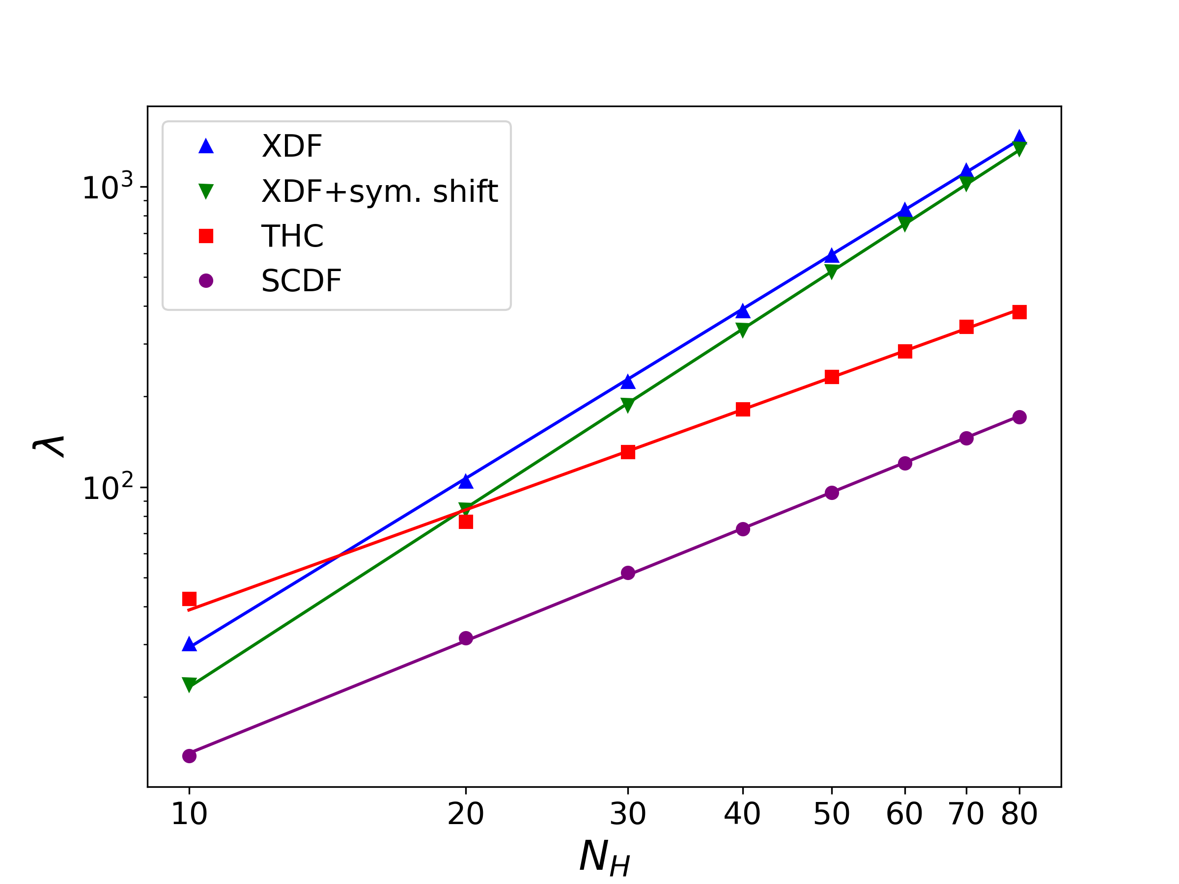
Figure 1: Scaling of the 1-norm $\lambda$ (in Ha) as a function of the number of hydrogen atoms $N_{H}$ for XDF, XDF with symmetry shift, THC, and SCDF.

Approach	$\lambda$		Number Toffolis		Number logical qubits
	Slope	$R^{2}$	Slope	$R^{2}$	Slope	$R^{2}$
XDF	1.87	0.9998	3.08	0.9997	1.27	0.9647
XDF+sym. shift	1.98	0.9999	3.18	0.9998	1.27	0.9647
THCa	1.11	0.9991	2.08	0.9998	1.01	0.9653
SCDF	1.24	0.9998	2.38	0.9998	1.21	0.9249
a Results obtained using the data provided with Ref. 21.

Table 5: Slopes of the linear fits on a logarithmic scale of the 1-norm $\lambda$, the number of Toffoli gates, and the number of logical qubits as a function of the number of hydrogen atoms N_H.

The behavior of the number of logical qubits as a function of the system size is less smooth and the fitting on a logarithmic scale in Table 5 and the right panel of Fig. 2 has to be considered as only indicative of the overall trends. Since the number of logical qubits has only a weak dependence on the 1-norm, in this case, the behaviors of the SCDF does not significantly differ with respect to XDF, and, as in the previous examples, THC has a lower requirements than the DF methods.

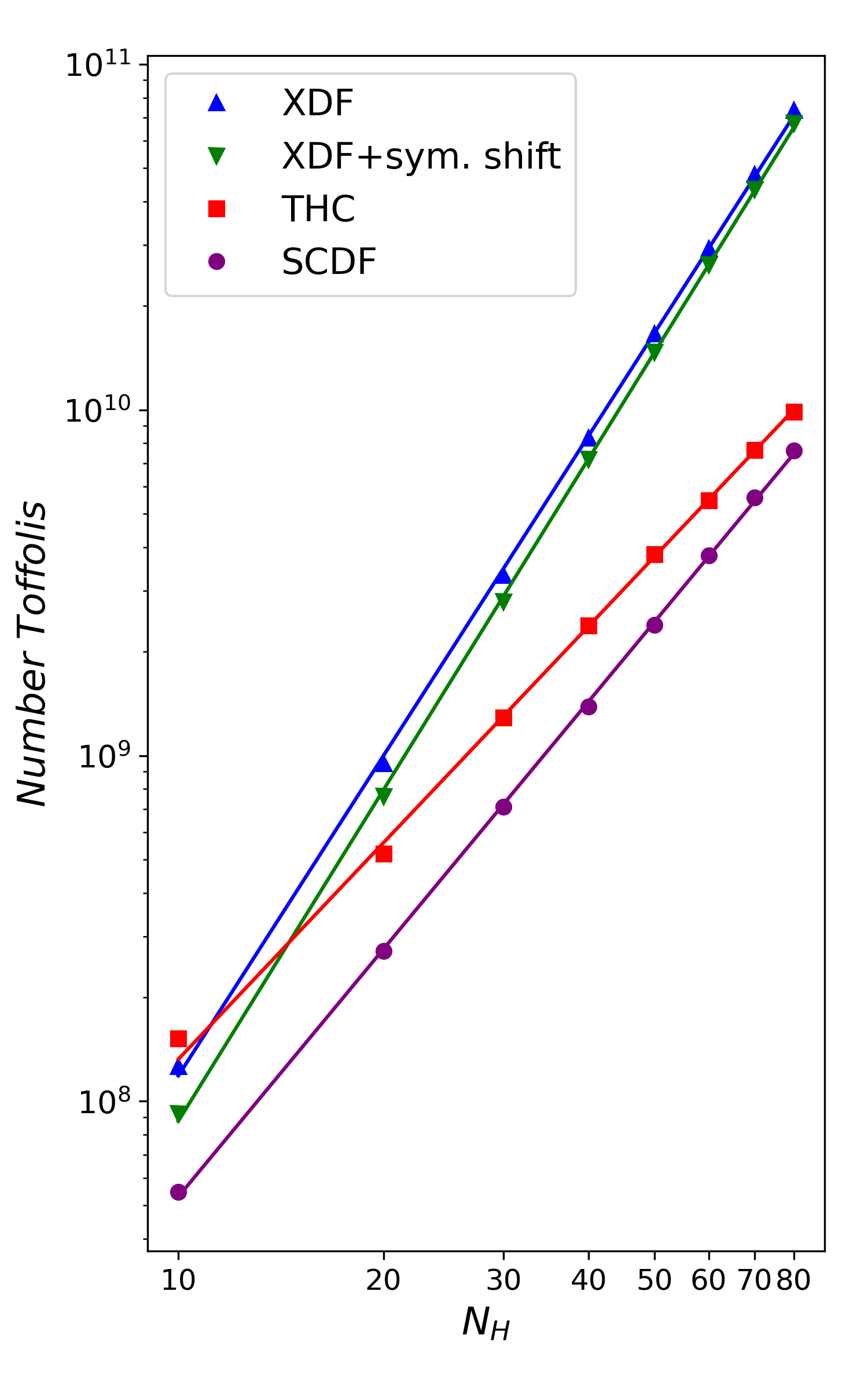
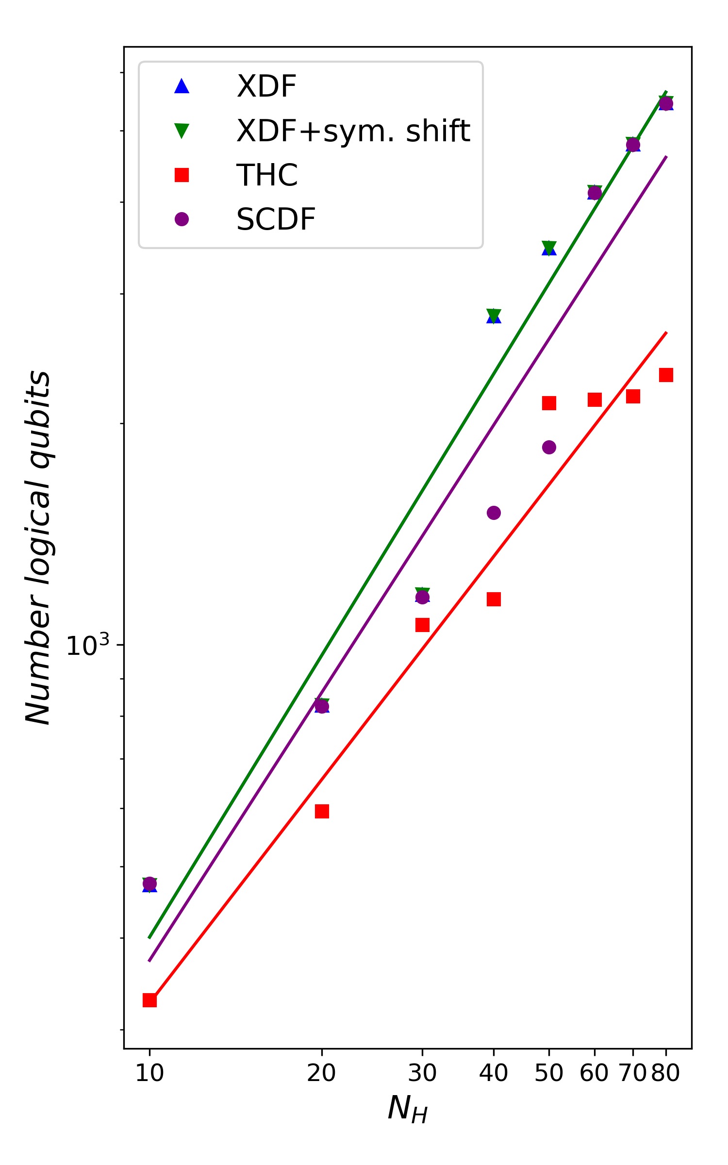
Figure 2: Left: Scaling of the number of Toffoli gates required by the XDF, XDF with symmetry shift, THC, and SCDF approaches as a function of the number of hydrogens $N_{H}$. Right: Scaling of the number of logical qubits.

4 Conclusions

In conclusion, we have introduced the symmetry-compressed double factorization approach that couples the symmetry shift technique with regularized double factorization to decrease the 1-norm of the electronic Hamiltonian significantly. As the 1-norm determines the total number of iterations needed in QPE, its reduction is important in decreasing the resource requirements and the runtime of fault-tolerant quantum simulations in chemistry. The effectiveness of the SCDF method in reducing the 1-norm is demonstrated numerically with applications to different chemical systems, including active space models of the FeMoco molecule, cytochrome P450, and hydrogen chains up to 80 atoms. For these systems, the 1-norm values achieved by SCDF are significantly lower than other methods, including XDF, XDF with symmetry shift, RCDF, and THC.

Despite the fundamental role of the 1-norm, other factors should also be taken into account to assess the performance of a specific Hamiltonian factorization in the context of qubitization-based QPE.

First, the cost of a single QPE iteration, which depends on the specific implementation and the number of terms in the Hamiltonian, can significantly impact the global computational cost. To perform an unbiased comparison of methods, the Toffoli gate and logical qubit requirements were estimated for the chemical systems considered here. This shows that SCDF still outperforms all the other methods regarding Toffoli gate counts. For example, for the FeMoco molecule and cytochrome P450, SCDF requires fewer than 50% of the Toffoli gates compared to THC, thus far recognized as the best-performing method in the literature. However, the number of terms in the THC-factorized Hamiltonian grows with lower complexity as compared to all other methods, and this approach will tend to become the most efficient for systems of growing size. Concerning the logical qubit count, SCDF inherits the same behavior as the other DF-based approaches, and tends to require relatively large numbers of qubits.

Second, given that Hamiltonian factorizations frequently employ tensor truncations to enhance efficiency, it is crucial to determine their impact on the ground-state total energy. We considered CCSD(T) correlation energies as an accuracy metric consistent with prior literature. Despite the potentially disruptive effect of the regularization, SCDF maintains a high level of accuracy comparable to other DF methods. The behavior of THC is more problematic. For example, in the case of cytochrome P450 the error in the correlation energy exhibits an erratic behavior as a function of the THC rank, with a tendency to significantly increase after reaching very small values. The behavior of the correlation energy is also nonsystematic as a function of the size of the hydrogen chains, and, in at least one case, the error significantly exceeds the chemical accuracy threshold.

In this work, the significant 1-norm reduction provided by SCDF has been exclusively exploited in the context of QPE. However, different quantum algorithms could benefit from the 1-norm decrease. This is the case, for example, of the stochastic compilation protocol known as qDRIFT ⁵³, which requires $O(\lambda^{2})$ repetitions to approximate the time evolution. The number of shots required to measure the expectation value of the Hamiltonian also grows with the 1-norm and, accordingly, also VQE and other near-term quantum algorithms could benefit from its reduction. Establishing the accuracy and efficiency of SCDF, also for near-term quantum algorithms, will be the subject of future work. In the context of fault-tolerant quantum computing, the ideas developed in this work may also apply within the THC framework. While not straightforward, this extension could lead to a highly efficient methodology with optimal scaling.

Appendix A Optimization of the SCDF cost function

The SCDF cost function in Eq. 27 has to be minimized with respect to the components of the $\mathbf{W}^{t}$, $\mathbf{U}^{t}$, and $\alpha^{t}$ tensors. As previously discussed for CDF ²⁸, the simultaneous optimization of the different tensors is inefficient and a nested approach with multiple steps should be preferred. For the SCDF cost function the optimization is performed through the following steps:

1. Optimization of the $\mathbf{W}^{t}$ tensor using the unconstrained minimization L-BFGS algorithm;

2. Update of the $\alpha^{t}$ values as median of the new $\mathbf{V}^{t}$;

3. Optimization of the $\mathbf{U}^{t}$ tensor using the L-BFGS algorithm.

4. Repeat from step 1 until convergence is achieved.

For the optimizations in steps 1 and 3 we have developed two different implementations based on analytical gradients and automatic differentiation using the JAX library ⁴⁸. While the former implementation is mainly intended to provide a reference and to test the soundness of the numerics, the latter is significantly more efficient and is used in production runs. The convergence criterion in step 4 is naturally defined in terms of thresholds on gradients or on the decrease of the cost function between subsequent iterations. However, since the 1-norm reduction is crucial to enhance the QPE efficiency and its value is found to decrease monotonically as a function of the iteration count, the optimization procedure was stopped only when the 1-norm value was steadily decreasing well below the 0.05 Ha threshold.

The analytical gradient of the SCDF cost function with respect to the components of the $\mathbf{W}^{t}$ tensor is given by

$$\frac{\partial\mathcal{L}^{\textrm{SCDF}}}{\partial W_{k}^{t}} = -2\sum_{p,q,r,s=1}^{N}\sum_{l=1}^{N}\Delta_{pqrs}U^{t}_{pk}U^{t}_{qk}W_{l}^{t}U^{t}_{rl}U^{t}_{sl}+2\rho\sum_{l=1}^{N}\text{sign}(W_{k}^{t}W_{l}^{t}-\alpha^{t})W_{l}^{t}$$ (28)

where

$$\Delta_{pqrs}\equiv(pq|rs)-\sum_{t=1}^{N_{\textrm{DF}}}\sum_{k,l=1}^{N}U^{t}_{pk}U^{t}_{qk}W_{k}^{t}W_{l}^{t}U^{t}_{rl}U^{t}_{sl}.$$ (29)

The analytical gradient of the SCDF cost function with respect to the components of $\mathbf{U}^{t}$ is given by

$$\frac{\partial\mathcal{L}^{\textrm{SCDF}}}{\partial U_{pk}^{t}} = -4\sum_{q,r,s=1}^{N}\sum_{l=1}^{N}\Delta_{pqrs}U^{t}_{qk}W_{l}^{t}U^{t}_{rl}U^{t}_{sl}.$$ (30)

Since the regularization term does not depend on the the $\mathbf{U}^{t}$ tensors this derivative is the same as for the CDF and RCDF approaches. The optimization of $\mathbf{U}^{t}$ is more complex than in the $\mathbf{W}^{t}$ case since this tensor has to be constrained to be orthogonal. In practice this problem can be formulated as an unconstrained optimization by introducing the antisymmetric orbital rotation generators matrices $\mathbf{X}^{t}$ to define $\mathbf{U}^{t}=\exp(\mathbf{X}^{t})$. The minimization of the cost function is then performed with respect to the components of $\mathbf{X}^{t}$; the procedure is described in detail in Ref. 28.

The minimization of the SCDF cost function is susceptible to the presence of local minima. Significantly lower values of the SCDF cost function and 1-norm can be found if very tight values ($10^{-12}$) are used for the tolerance of the stopping criterion of the L-BFGS algorithm. However, this approach requires a large number of iterations for each minimization of $\mathbf{W}^{t}$ and $\mathbf{U}^{t}$, and the overall optimization is slow.

Appendix B Quantum implementation of the symmetry-compressed double factorized Hamiltonian

The implementation of the (rank 1) double factorized Hamiltonian in the form of Eq. 14 has been discussed in details in Ref. 24. Specifically, this approach is valid for a positive definite/rank one $\mathbf{V}^{t}$ tensor, as in the XDF case. In this appendix we show that the implementation of SCDF requires minimal modifications with respect to the original work of von Burg et al.. Within the SCDF framework, Eq. 25 redefines the two-body part of the Hamiltonian by introducing a symmetry shift of each term in the sum over the index $t$, leading to the following form of Eq. 8:

$$\hat{H}=E_{\textrm{nuc}}+\sum_{p,q=1}^{N}k_{pq}\hat{E}_{pq}+\frac{1}{2}\sum_{t=1}^{N_{\textrm{DF}}}\sum_{k,l=1}^{N}(V^{t}_{kl}-\alpha^{t})\hat{G}_{t}^{{\dagger}}\hat{E}_{kk}\hat{E}_{ll}\hat{G}_{t}.$$ (31)

As shown by the numerical applications part in Sec. 3, the values of $\alpha^{t}$ are actually different from zero only for a small number $N_{\alpha}$ of indexes $t$. In SCDF $\mathbf{V}^{t}=\mathbf{W}^{t}\otimes\mathbf{W}^{t}$ is rank 1 and the element-wise constant shift $\alpha^{t}$ is equivalent to subtracting the rank 1 tensor $-\alpha^{t}\mathbf{1}\otimes\mathbf{1}$ (here $\otimes$ denotes the outer product and $\mathbf{1}$ is a vector whose $N$ components are all 1). This implies that $\mathbf{V}^{t}-\alpha^{t}$ has rank two and, by applying an eigenvalue decomposition, can be expressed as

$$\mathbf{V}^{t}-\alpha^{t}=\mathbf{P}^{t}\otimes\mathbf{P}^{t}-\mathbf{Q}^{t}\otimes\mathbf{Q}^{t},$$ (32)

where $\mathbf{P}^{t}$ and $\mathbf{Q}^{t}$ are 1D tensors. To keep the formalism consistent, in this appendix we will define $\mathbf{P}^{t}=\mathbf{W}^{t}$ and $\mathbf{Q}^{t}=\mathbf{0}$ for the $t$ indexes corresponding to $\alpha^{t}=0$ (or, more precisely, corresponding to the $\alpha^{t}$’s smaller than a given threshold $\delta_{\alpha}$). The application of the Jordan-Wigner transformation to the Hamiltonian in Eq. 31 leads to

$$\hat{H}=\!\!\!\!\!\!\! \mathcal{E}-\frac{1}{2}\sum_{k=1}^{N}f^{\text{\o}}_{k}G_{\text{\o}}^{{\dagger}}(\hat{Z}_{k}+\hat{Z}_{\bar{k}})G_{\text{\o}}$$ (33)

$$+\frac{1}{8}\sum_{t=1}^{N_{\textrm{DF}}}\hat{G}_{t}^{{\dagger}}\left(\sum_{k=1}^{\Xi^{(t)}}P^{t}_{k}(\hat{Z}_{k}+\hat{Z}_{\bar{k}})\right)^{2}\hat{G}_{t}-\frac{1}{8}\sideset{}{{}^{\prime}}{\sum}_{t=1}^{N_{\textrm{DF}}}\hat{G}_{t}^{{\dagger}}\left(\sum_{k=1}^{\Theta^{(t)}}Q^{t}_{k}(\hat{Z}_{k}+\hat{Z}_{\bar{k}})\right)^{2}\hat{G}_{t},$$

where the primed sum $\sideset{}{{}^{\prime}}{\sum}$ indicates that only the $N_{\alpha}$ non-zero terms are actually included. Similarly to Eq. 14, a threshold $\delta_{\textrm{DF}}$ is applied to eliminate the small components of the $\mathbf{P}^{t}$ and $\mathbf{Q}^{t}$ tensors; this leads to sums over $k$ that run up to values $\Xi^{(t)}$ and $\Theta^{(t)}$ that are less than or equal to $N$. This equation is analogous to the formulation of von Burg et al. in Eq. 14, with only $N_{\alpha}$ additional terms with a negative sign. The implementation of terms with a negative sign requires minimal modifications with respect to the implementation described in the supporting information (SI) of Ref. 24. The minus sign can be included when combining the two body terms evaluated from qubitization. Using the same notation of the SI of Ref. 24, this can be achieved by replacing $\left|\overrightarrow{\Lambda_{SH}}\right\rangle^{\dagger}$ with $\overline{\left|\overrightarrow{\Lambda_{SH}}\right\rangle}^{\ {\dagger}}$ in the circuit in Eq. 78 therein. The notation with an additional line on top is used in Ref. 24 to distinguish Eqs. 7 and 8, which correspond to the prepare operator for block encoding without or with sign, respectively. The quantum circuits for $\left|\overrightarrow{\Lambda_{SH}}\right\rangle^{\dagger}$ and $\overline{\left|\overrightarrow{\Lambda_{SH}}\right\rangle}^{\ {\dagger}}$ are very similar and require the same number of Toffoli gates. Accordingly, the required resources are not affected by the negative sign and the resource estimation was carried out using the standard OpenFermion implementation ⁴⁹.

References

- Heifetz 2020 Heifetz, A. Quantum mechanics in drug discovery; Springer, 2020
- Nørskov et al. 2009 Nørskov, J. K.; Bligaard, T.; Rossmeisl, J.; Christensen, C. H. Towards the computational design of solid catalysts. Nature chemistry 2009, 1, 37–46
- Jain et al. 2013 Jain, A.; Ong, S. P.; Hautier, G.; Chen, W.; Richards, W. D.; Dacek, S.; Cholia, S.; Gunter, D.; Skinner, D.; Ceder, G.; others Commentary: The Materials Project: A materials genome approach to accelerating materials innovation. APL materials 2013, 1
- Cao et al. 2019 Cao, Y.; Romero, J.; Olson, J. P.; Degroote, M.; Johnson, P. D.; Kieferová, M.; Kivlichan, I. D.; Menke, T.; Peropadre, B.; Sawaya, N. P. D.; Sim, S.; Veis, L.; Aspuru-Guzik, A. Quantum Chemistry in the Age of Quantum Computing. Chemical Reviews 2019, 119, 10856–10915
- Peruzzo et al. 2014 Peruzzo, A.; McClean, J.; Shadbolt, P.; Yung, M.-H.; Zhou, X.-Q.; Love, P. J.; Aspuru-Guzik, A.; O’brien, J. L. A variational eigenvalue solver on a photonic quantum processor. Nature communications 2014, 5, 4213
- Tilly et al. 2022 Tilly, J.; Chen, H.; Cao, S.; Picozzi, D.; Setia, K.; Li, Y.; Grant, E.; Wossnig, L.; Rungger, I.; Booth, G. H.; others The variational quantum eigensolver: a review of methods and best practices. Physics Reports 2022, 986, 1–128
- goo 2023 Suppressing quantum errors by scaling a surface code logical qubit. Nature 2023, 614, 676–681
- Bluvstein et al. 2023 Bluvstein, D.; Evered, S. J.; Geim, A. A.; Li, S. H.; Zhou, H.; Manovitz, T.; Ebadi, S.; Cain, M.; Kalinowski, M.; Hangleiter, D.; others Logical quantum processor based on reconfigurable atom arrays. Nature 2023, 1–3
- 9 {https://newsroom.ibm.com/2023-12-04-IBM-Debuts-Next-Generation-Quantum-Processor-IBM-Quantum-System-Two,-Extends-Roadmap-to-Advance-Era-of-Quantum-Utility}
- 10 {https://quantumai.google/qecmilestone}
- Abrams and Lloyd 1999 Abrams, D. S.; Lloyd, S. Quantum algorithm providing exponential speed increase for finding eigenvalues and eigenvectors. Physical Review Letters 1999, 83, 5162
- Aspuru-Guzik et al. 2005 Aspuru-Guzik, A.; Dutoi, A. D.; Love, P. J.; Head-Gordon, M. Simulated quantum computation of molecular energies. Science 2005, 309, 1704–1707
- Suzuki 1993 Suzuki, M. Improved Trotter-like formula. Physics Letters A 1993, 180, 232–234
- Berry et al. 2015 Berry, D. W.; Childs, A. M.; Cleve, R.; Kothari, R.; Somma, R. D. Simulating Hamiltonian dynamics with a truncated Taylor series. Physical review letters 2015, 114, 090502
- Berry et al. 2018 Berry, D. W.; Kieferová, M.; Scherer, A.; Sanders, Y. R.; Low, G. H.; Wiebe, N.; Gidney, C.; Babbush, R. Improved techniques for preparing eigenstates of fermionic Hamiltonians. npj Quantum Information 2018, 4, 22
- Poulin et al. 2018 Poulin, D.; Kitaev, A.; Steiger, D. S.; Hastings, M. B.; Troyer, M. Quantum algorithm for spectral measurement with a lower gate count. Physical review letters 2018, 121, 010501
- Babbush et al. 2018 Babbush, R.; Gidney, C.; Berry, D. W.; Wiebe, N.; McClean, J.; Paler, A.; Fowler, A.; Neven, H. Encoding electronic spectra in quantum circuits with linear T complexity. Physical Review X 2018, 8, 041015
- Low and Chuang 2019 Low, G. H.; Chuang, I. L. Hamiltonian simulation by qubitization. Quantum 2019, 3, 163
- Bravyi and Kitaev 2005 Bravyi, S.; Kitaev, A. Universal quantum computation with ideal Clifford gates and noisy ancillas. Physical Review A 2005, 71, 022316
- Reichardt 2005 Reichardt, B. W. Quantum universality from magic states distillation applied to CSS codes. Quantum Information Processing 2005, 4, 251–264
- Lee et al. 2021 Lee, J.; Berry, D. W.; Gidney, C.; Huggins, W. J.; McClean, J. R.; Wiebe, N.; Babbush, R. Even more efficient quantum computations of chemistry through tensor hypercontraction. PRX Quantum 2021, 2, 030305
- Low et al. 2018 Low, G. H.; Kliuchnikov, V.; Schaeffer, L. Trading T-gates for dirty qubits in state preparation and unitary synthesis. arXiv preprint arXiv:1812.00954 2018,
- Berry et al. 2019 Berry, D. W.; Gidney, C.; Motta, M.; McClean, J. R.; Babbush, R. Qubitization of arbitrary basis quantum chemistry leveraging sparsity and low rank factorization. Quantum 2019, 3, 208
- von Burg et al. 2021 von Burg, V.; Low, G. H.; Häner, T.; Steiger, D. S.; Reiher, M.; Roetteler, M.; Troyer, M. Quantum computing enhanced computational catalysis. Physical Review Research 2021, 3, 033055
- Motta et al. 2021 Motta, M.; Ye, E.; McClean, J. R.; Li, Z.; Minnich, A. J.; Babbush, R.; Chan, G. K.-L. Low rank representations for quantum simulation of electronic structure. npj Quantum Information 2021, 7, 83
- Kivlichan et al. 2018 Kivlichan, I. D.; McClean, J.; Wiebe, N.; Gidney, C.; Aspuru-Guzik, A.; Chan, G. K.-L.; Babbush, R. Quantum simulation of electronic structure with linear depth and connectivity. Physical review letters 2018, 120, 110501
- Huggins et al. 2021 Huggins, W. J.; McClean, J. R.; Rubin, N. C.; Jiang, Z.; Wiebe, N.; Whaley, K. B.; Babbush, R. Efficient and noise resilient measurements for quantum chemistry on near-term quantum computers. npj Quantum Information 2021, 7, 23
- Cohn et al. 2021 Cohn, J.; Motta, M.; Parrish, R. M. Quantum filter diagonalization with compressed double-factorized hamiltonians. PRX Quantum 2021, 2, 040352
- Oumarou et al. 2022 Oumarou, O.; Scheurer, M.; Parrish, R. M.; Hohenstein, E. G.; Gogolin, C. Accelerating Quantum Computations of Chemistry Through Regularized Compressed Double Factorization. arXiv preprint arXiv:2212.07957 2022,
- Rubin et al. 2022 Rubin, N. C.; Lee, J.; Babbush, R. Compressing many-body fermion operators under unitary constraints. Journal of Chemical Theory and Computation 2022, 18, 1480–1488
- Hohenstein et al. 2012 Hohenstein, E. G.; Parrish, R. M.; Martínez, T. J. Tensor hypercontraction density fitting. I. Quartic scaling second-and third-order Møller-Plesset perturbation theory. The Journal of chemical physics 2012, 137
- Parrish et al. 2012 Parrish, R. M.; Hohenstein, E. G.; Martínez, T. J.; Sherrill, C. D. Tensor hypercontraction. II. Least-squares renormalization. The Journal of chemical physics 2012, 137
- Goings et al. 2022 Goings, J. J.; White, A.; Lee, J.; Tautermann, C. S.; Degroote, M.; Gidney, C.; Shiozaki, T.; Babbush, R.; Rubin, N. C. Reliably assessing the electronic structure of cytochrome p450 on today’s classical computers and tomorrow’s quantum computers. Proceedings of the National Academy of Sciences 2022, 119, e2203533119
- Koridon et al. 2021 Koridon, E.; Yalouz, S.; Senjean, B.; Buda, F.; O’Brien, T. E.; Visscher, L. Orbital transformations to reduce the 1-norm of the electronic structure Hamiltonian for quantum computing applications. Physical Review Research 2021, 3, 033127
- Loaiza et al. 2022 Loaiza, I.; Marefat Khah, A.; Wiebe, N.; Izmaylov, A. F. Reducing molecular electronic hamiltonian simulation cost for linear combination of unitaries approaches. Quantum Science and Technology 2022,
- Jordan and Wigner 1928 Jordan, P.; Wigner, E. On Paul’s prohibition on equivalence. Zeitschrift Physik 1928, 631–651
- Bravyi and Kitaev 2002 Bravyi, S. B.; Kitaev, A. Y. Fermionic quantum computation. Annals of Physics 2002, 298, 210–226
- Seeley et al. 2012 Seeley, J. T.; Richard, M. J.; Love, P. J. The Bravyi-Kitaev transformation for quantum computation of electronic structure. The Journal of chemical physics 2012, 137
- Poulin et al. 2014 Poulin, D.; Hastings, M. B.; Wecker, D.; Wiebe, N.; Doherty, A. C.; Troyer, M. The Trotter step size required for accurate quantum simulation of quantum chemistry. arXiv preprint arXiv:1406.4920 2014,
- Matsuzawa and Kurashige 2020 Matsuzawa, Y.; Kurashige, Y. Jastrow-type decomposition in quantum chemistry for low-depth quantum circuits. Journal of chemical theory and computation 2020, 16, 944–952
- Thouless 1960 Thouless, D. J. Stability conditions and nuclear rotations in the Hartree-Fock theory. Nuclear Physics 1960, 21, 225–232
- Childs and Wiebe 2012 Childs, A. M.; Wiebe, N. Hamiltonian simulation using linear combinations of unitary operations. arXiv preprint arXiv:1202.5822 2012,
- Dunlap et al. 1979 Dunlap, B. I.; Connolly, J.; Sabin, J. On some approximations in applications of X theory. The Journal of Chemical Physics 1979, 71, 3396–3402
- Werner et al. 2003 Werner, H.-J.; Manby, F. R.; Knowles, P. J. Fast linear scaling second-order Møller-Plesset perturbation theory (MP2) using local and density fitting approximations. The Journal of chemical physics 2003, 118, 8149–8160
- Pedersen et al. 2009 Pedersen, T. B.; Aquilante, F.; Lindh, R. Density fitting with auxiliary basis sets from Cholesky decompositions. Theoretical Chemistry Accounts 2009, 124, 1–10
- Hohenstein and Sherrill 2010 Hohenstein, E. G.; Sherrill, C. D. Density fitting of intramonomer correlation effects in symmetry-adapted perturbation theory. The Journal of chemical physics 2010, 133
- Loaiza and Izmaylov 2023 Loaiza, I.; Izmaylov, A. F. Reducing the molecular electronic Hamiltonian encoding costs on quantum computers by symmetry shifts. arXiv preprint arXiv:2304.13772 2023,
- Bradbury et al. 2018 Bradbury, J.; Frostig, R.; Hawkins, P.; Johnson, M. J.; Leary, C.; Maclaurin, D.; Necula, G.; Paszke, A.; VanderPlas, J.; Wanderman-Milne, S.; Zhang, Q. JAX: composable transformations of Python+NumPy programs. 2018; http://github.com/google/jax
- McClean et al. 2020 McClean, J. R.; Rubin, N. C.; Sung, K. J.; Kivlichan, I. D.; Bonet-Monroig, X.; Cao, Y.; Dai, C.; Fried, E. S.; Gidney, C.; Gimby, B.; others OpenFermion: the electronic structure package for quantum computers. Quantum Science and Technology 2020, 5, 034014
- Beinert et al. 1997 Beinert, H.; Holm, R. H.; Munck, E. Iron-sulfur clusters: nature’s modular, multipurpose structures. Science 1997, 277, 653–659
- Reiher et al. 2017 Reiher, M.; Wiebe, N.; Svore, K. M.; Wecker, D.; Troyer, M. Elucidating reaction mechanisms on quantum computers. Proceedings of the national academy of sciences 2017, 114, 7555–7560
- Li et al. 2019 Li, Z.; Li, J.; Dattani, N. S.; Umrigar, C.; Chan, G. K. The electronic complexity of the ground-state of the FeMo cofactor of nitrogenase as relevant to quantum simulations. The Journal of chemical physics 2019, 150
- Campbell 2019 Campbell, E. Random compiler for fast Hamiltonian simulation. Physical review letters 2019, 123, 070503