Role of long jumps in Lévy noise induced multimodality

Abstract

Lévy noise is a paradigmatic noise used to describe out-of-equilibrium systems. Typically, properties of Lévy noise driven systems are very different from their Gaussian white noise driven counterparts. In particular, under action of Lévy noise, stationary states in single-well, super-harmonic, potentials are no longer unimodal. Typically, they are bimodal however for fine-tuned potentials the number of modes can be further increased. The multimodality arises as a consequence of the competition between long displacements induced by the non-equilibrium stochastic driving and action of the deterministic force. Here, we explore robustness of bimodality in the quartic potential under action of the Lévy noise. We explore various scenarios of bounding long jumps and assess their ability to weaken and disassembly multimodality. In general, we demonstrate that despite its robustness it is possible to destroy the bimodality by limiting the length of noise-induced jumps.

Increasing number of observations demonstrates plethora of situations in which non-Gaussian heavy tailed fluctuations are recorded. This indicates the need to include heavy-tailed fluctuations in the description of dynamical systems especially in out-of-equilibrium realms. The possibility of anomalously long jumps, drastically changes the properties of stochastic dynamical systems compared to their Gaussian noise driven counterparts. It is the long jumps that lead to bimodal non-equilibrium stationary states in single-well, super-harmonic, potential wells. Exploration of different scenarios for restricting long jumps, allows for a better understanding of how long jumps determine the properties of stationary states and how they affect their modality. This provides a deeper understanding of the role of non-Gaussian long jumps and the mechanisms responsible for emergence of multimodal stationary states.

I Introduction

The motion in complex environments can be efficiently approximated by methods of stochastic dynamics Schimansky-Geier and Pöshel (1997); Klafter et al. (2012); Tomé and De Oliveira (2016), which incorporates stochastic processes into equations describing the system’s dynamics. The noise is used to efficiently and effectively approximate complex, not fully known interactions of the test particle with its environment. The stochastic dynamics in a fixed potential is capable of producing bimodal stationary states. Multimodal stationary states can emerge in multi-well potentials $V(x)$ under action of the additive Gaussian white noise (GWN), what is evident from the fact that stationary state Gardiner (2009); Risken (9996); Reichl (1998) in such a case is $p(x)\sim\exp\left[-\beta V(x)\right]$. This, somewhat obvious, mechanism corresponds to motion in an appropriately prepared medium in the equilibrium environment. However, there are various mechanisms that can lead to emergence of multimodal stationary states which do not rely on the shape of the potential. The less intuitive, but more intriguing, approach involves utilizing different noise types to control the existence and modality of stationary states. Such a setup allows one to obtain multimodal stationary states even in a single-well potential if the noise component is chosen appropriately. For instance, Lévy noise Chechkin et al. (2002a, 2003); Cieśla et al. (2019); Capała and Dybiec (2019), Ornstein–Uhlenbeck noise Jacquet et al. (2018) and fractional Gaussian noise Guggenberger et al. (2021) can lead to emergence of bimodal stationary states in the single-well potential.

Among above mentioned drivings, only in the case of Lévy noise, are the long jumps expected to play the crucial role in formation of multimodal stationary states, because under action of Ornstein–Uhlenbeck and fractional Gaussian noises the multimodality is thought to be induced by the interplay of the correlation of the noise driven motion Jacquet et al. (2018); Guggenberger et al. (2021) and the action of the deterministic force. A very different situation is observed for the Lévy noise Chechkin et al. (2006, 2008) which is of particular interest to our studies. The Lévy noise is used to approximate out-of-equilibrium systems Dubkov et al. (2008); Dybiec and Gudowska-Nowak (2009) displaying heavy-tailed fluctuations Solomon et al. (1993, 1994); del Castillo-Negrete (1998); Shlesinger et al. (1993); Klafter et al. (1996); Chechkin et al. (2002b); del Castillo-Negrete et al. (2005); Katori et al. (1997); Peng et al. (1993); Segev et al. (2002); Lomholt et al. (2005); Viswanathan et al. (1996); Brockmann et al. (2006). It is capable of producing bimodal stationary states in super-harmonic, single-well potentials Chechkin et al. (2002a, 2003). Clearly, in order to produce a bimodal stationary state in a single-well symmetric potential (under action of a symmetric noise), at the origin there has to be a minimum of stationary density. Therefore, there must be a mechanism producing a deficit of the probability mass at the origin. More precisely, under Lévy driving, the multimodality is known to originate due to competition between two components of the system dynamics: (i) long stochastic jumps and (ii) deterministic sliding to the origin, which could be characterized by the diverging time. Long jumps resulting in visits to distant points are produced by the heavy-tailed, Lévy noise, while sliding to the origin is defined by the deterministic force. In a situation when a particle almost never returns to the origin before performing the next long jump the stationary density becomes bimodal. Therefore, in the context of long jumps, a natural question arises: how long “long jumps” are needed in order to induce a multimodal stationary state in a single-well potential?

To explore the role of longs jumps on the formation of multimodal stationary states in a single-well potentials, we first enclose the system at hand in a box and investigate how the stationary states are affected by the box size and the way how the box edges interact with the system dynamics. This can be done in at least two ways: first by introducing reflecting boundaries (“reflection scheme”), second by rejecting jumps which would move the particle outside the box (“rejection scheme”). Within the current study, we extensively compare both above mentioned options with respect to their role on the formation and robustness of bimodality. Lastly, we provide comparison with the case of a truncated jump length distribution. These scenarios significantly differ from reduction of spread of particles due to stochastic resetting Evans and Majumdar (2011); Evans et al. (2020); Gupta and Jayannavar (2022), as (except for the “truncation scheme”) they directly limit the accessible space which subsequently results in indirect modification of the jump length distribution.

The model under study is described in the next section (Sec. II – Models). Obtained results are included in the Sec. III – Results and Discussion. The paper is completed by Sec IV – Summary and Conclusions. Additional information is moved to appendices: A ($\alpha$-stable random variables and Lévy noise) and B (Deterministic sliding).

II Models

We study the general system described by the overdamped Langevin equation

$$\frac{dx}{dt}=-V^{\prime}(x)+\xi(t),$$ (1)

where

$$V(x)=\frac{1}{c}|x|^{c}\;\;\;\;\;(c>0)$$ (2)

is the single-well, power-law potential and $\xi(t)$ is a symmetric Lévy ($\alpha$-stable) noise. The $\alpha$-stable noise is a generalization of the Gaussian white noise to the non-equilibrium realms Janicki and Weron (1994), where heavy tailed fluctuations are abundant Ditlevsen (1999); Mercadier et al. (2009); Barkai et al. (2014); Amor et al. (2016); Barthelemy et al. (2008); Fioriti et al. (2015); Lera and Sornette (2018). The noise produces independent increments which follow a symmetric, unimodal, heavy-tailed $\alpha$-stable density Janicki and Weron (1994); Samorodnitsky and Taqqu (1994), i.e., probability density with the characteristic function $\varphi(k)=\exp\left[-\sigma^{\alpha}|k|^{\alpha}\right]$, where $\alpha$ ($0<\alpha\leqslant 2$) is the stability index controlling the asymptotics of the distribution, while $\sigma$ ($\sigma>0$) is the scale parameter Janicki and Weron (1994); Samorodnitsky and Taqqu (1994). For $\alpha=2$ one recovers the Gaussian white noise while for $\alpha<2$ the heavy-tailed, power-law, Lévy noise. For more details see Refs. Chechkin et al., 2002b, 2006; Dubkov et al., 2008 and App. A. The steepness of the potential, see Eq. (2), is controlled by the exponent $c$.

Under action of the Lévy noise the evolution of the probability density $p(x,t|x_{0},t_{0})$ is governed by the fractional Smoluchowski–Fokker–Planck equation Jespersen et al. (1999); Yanovsky et al. (2000); Schertzer et al. (2001)

$$\frac{\partial p}{\partial t}=\frac{\partial}{\partial x}\left[V^{\prime}(x)p\right]+\sigma^{\alpha}\frac{\partial^{\alpha}p}{\partial|x|^{\alpha}}.$$ (3)

The fractional Riesz–Weil $\frac{\partial^{\alpha}p}{\partial|x|^{\alpha}}$ derivative Podlubny (1999); Samko et al. (1993) is understood in the sense of the Fourier transform, which is natural for unbounded domains

$$\mathcal{F}_{k}\left(\frac{\partial^{\alpha}f(x)}{\partial|x|^{\alpha}}\right)=-|k|^{\alpha}\mathcal{F}_{k}(f(x)).$$ (4)

However, in more complex setups, e.g., escape from a finite interval, other types of space-fractional derivatives are used Podlubny (1999); Padash et al. (2019) and additional care with respect to definitions of fractional operators and boundary conditions is required Kwaśnicki (2017); Song et al. (2017); Cusimano et al. (2018). Subsequently, in the unbounded space, from Eq. (3), using the Fourier transform (characteristic function), the stationary state can be derived Chechkin et al. (2003, 2004).

Stationary states in systems driven by Lévy noises exist for potential wells which are steep enough Dybiec et al. (2010), i.e., $c>2-\alpha$. In even potentials $V(x)$, e.g., see Eq. (2), under action of symmetric noise they are symmetric. For $c=2$ (harmonic potential) they are given by the $\alpha$-stable density, from which noise pulses were taken, with a changed (rescaled) scale parameter Chechkin et al. (2002a, 2003); Dybiec et al. (2007), which is the consequence of linearity of the Langevin equation in this case. For $c>2$ stationary densities becomes bimodal Chechkin et al. (2002a, 2003); Dubkov and Spagnolo (2007); Capała and Dybiec (2019). In particular for $c=4$ and the Cauchy noise ($\alpha$-stable noise with $\alpha=1$) the non-equilibrium stationary density reads Chechkin et al. (2002a, 2003, 2004, 2006, 2008)

$$p_{\alpha=1}(x)=\frac{1}{\pi\sigma^{\frac{1}{3}}\left[\left(\frac{x}{\sqrt[3]{\sigma}}\right)^{4}-\left(\frac{x}{\sqrt[3]{\sigma}}\right)^{2}+1\right]}.$$ (5)

From Eq. (5) it is apparent that the stationary state is indeed a symmetric bimodal distribution with modes at

$$x_{mod}=\pm\sigma^{\frac{1}{3}}/\sqrt{2}$$ (6)

and the power-law asymptotics $p(|x|)\propto|x|^{-4}$. The limit $c\to\infty$, see Eq. (2), transforms the single-well potential into the infinite rectangular potential-well with boundaries located at $x=\pm 1$. In such a limit, the stationary density reads Denisov et al. (2008)

$$p_{\infty}(x)=\frac{\Gamma(\alpha)(2L)^{1-\alpha}(L^{2}-x^{2})^{\alpha/2-1}}{\Gamma^{2}(\alpha/2)}$$ (7)

with $L=1$. In contrast to the finite $c$, see Ref. Dubkov and Spagnolo, 2007, the stationary density (7) does not depend on the scale parameter $\sigma$. Moreover, modal values are located at boundaries, i.e., at $\pm 1$.

In order to assess the role of the long jumps on the emergence of bimodality we investigate three different ways of limiting jump lengths. In scenarios ($i$) and ($ii$), the potential $V(x)$ is immersed in a $[-L,L]$ box, of variable half-width $L$, which introduces boundaries at $\pm L$, while in ($iii$) the jump length distribution is truncated at $\pm L$:

• “reflection scheme”: we introduce reflecting (impenetrable) boundaries at $\pm L$. Too long jumps are shortened to reach at most $-L+\varepsilon$ and $L-\varepsilon$, see Ref. Dybiec et al., 2017, where $\varepsilon$ is a small ($\varepsilon\ll L$) positive parameter. Consequently, the particle always stays within the $[-L,L]$ box.

• “rejection case”: we again introduce boundaries at $\pm L$, but now every jump which would move the particle outside the $[-L,L]$ box is rejected. Such boundaries implement a space dependent truncation of the jump length distribution. Note that this makes the jump length distribution space dependent and in general asymmetric as a particle can initiate a jump from any $x\in(-L,L)$. Furthermore, jump lengths are neither independent nor identically distributed.

• “truncation scheme”: constraints are introduced by truncating the noise induced part of a jump at $\pm L$, that is jumps exceeding length $L$ are rejected. Therefore, contrary to previous schemes, the particle can leave the $[-L,L]$ interval in a series of jumps (for jumps starting at $x=0$) or even in a single jump (for jumps starting at $x\neq 0$).

Note, that the all considered schemes ultimately (directly or indirectly) affect the jump length distribution. For scenario ($i$) and ($ii$) this is done indirectly by boundary conditions, while for ($iii$) the truncation is explicit.

The Langevin equation (1) was integrated using the Euler-Maruyama method Higham (2001); Mannella (2002)

$$x(t+\Delta t)=x(t)-V^{\prime}(x)\Delta t+\xi_{t}\Delta t^{1/\alpha},$$ (8)

with the integration time step $\Delta t=10^{-3}$. The integration time step $\Delta t$ was tested for self-consistency of the results. Moreover, we have verified that for the uninterrupted motion the theoretical stationary states (the quartic potential with the Cauchy noise, see Eq. (5), and the infinite rectangular potential well, see Eq. (7)) are correctly reconstructed. The realizations of independent and identically distributed random variables $\xi_{t}$ following the symmetric $\alpha$-stable distributions have been generated using the GNU Scientific Library implementation of general methods Chambers et al. (1976); Weron (1996) of generation of $\alpha$-stable random variables. Nevertheless, studies have been limited to the Cauchy case ($\alpha$-stable density with $\alpha=1$) for which the general method Chambers et al. (1976); Weron (1996), reduces to the inversion of the cumulative density. Additionally, we assume that the scale parameter $\sigma$ is set to $\sigma=1$. Scenarios ($ii$) and ($iii$) are realized by drawing jumps until the restraint condition is satisfied. Such an approach corresponds to the so-called “accept-reject” method of generating (pseudo) random numbers Devroye (1986); Newman and Barkema (1999). Main numerical results have been averaged over $10^{7}$ (“truncation”), $2\times 10^{7}$ (“reflection”) and $10^{8}$ (“rejection”) trajectories. Simulation time was adjusted in such a way that the stagnation of interquantile distance is observed, indicating that the stationary state has been reached. Finally, in the “reflection scheme” $\varepsilon=10^{-3}$ was used, as it is small enough to assure that in the infinite rectangular potential well the numerically constructed stationary state is given by Eq. (7).

III Results and discussion

Here, we present numerical results exploring properties of stationary states corresponding to three different schemes of restricting jump lengths described in Sec. II. In all cases, the magnitude of the restoring force $-V^{\prime}(x)$ is implicitly reduced, because visits to points where the deterministic force is large are either limited or fully eliminated. Moreover, the potential, see Eq. (2), boundaries (scenario ($i$) and ($ii$)) and truncation (scenario ($iii$)) are symmetric. Therefore obtained stationary states are symmetric as well, i.e., $p(x)=p(-x)$. Following subsections correspond to: “reflection scheme” (Sec. III.1), “rejection scheme” (Sec. III.2) and “truncation scheme” (Sec. III.3).

Figure 1: Stationary probability densities for the quartic potential ($c=4$ in Eq. (2)) with different values of $L$ under “reflection scheme” . Jumps moving a particle to the exterior of $[-L,L]$ are terminated at $L-\varepsilon$ or $-L+\varepsilon$. $\varepsilon$ is set to $\varepsilon=10^{-3}$. Left part of the plot is presented in linear scale, while in the right part the semi-log scale is used. Thin solid lines show stationary density given by Eq. (7) with $L=0.6$.

III.1 Reflection scheme

The “reflection scheme” implements impenetrable boundary conditions Dybiec et al. (2017). On the level of the Langevin equation, this is accounted for by terminating jumps which would leave the $[-L,L]$ interval at $-L+\varepsilon$ or $L-\varepsilon$. As demonstrated in Refs. Dybiec et al., 2017 and Kharcheva et al., 2016, for sufficiently small $\varepsilon$, such an approach properly implements reflecting boundary conditions on the single trajectory level. In particular, it correctly recovers Dybiec et al. (2017) the stationary state in the infinite rectangular potential well, see Eq. (7). The infinite rectangular potential well can be also obtained as $c\to\infty$ limit of the single-well potential $V(x)$, see Eq. (2) and Refs. Dybiec et al., 2017; Kharcheva et al., 2016. Consequently, the stationary state in the $c\to\infty$ limit is the same as the one given by Eq. (7), see Refs. Dybiec et al., 2017; Kharcheva et al., 2016. The stationary state in the infinite rectangular box is always bimodal. The probability density monotonically grows with $|x|$ and reaches maxima near the boundaries. For not too wide box, the deterministic force $-V^{\prime}(x)$ in the $[-L,L]$ region is relatively small, and one could expect that once the box size $L$ becomes smaller than absolute value of modal value in the unrestricted space $x_{mod}$, i.e., $L<1/\sqrt{2}\approx 0.707$, modal values will be located approximately at $\pm L$. However, it turns out that the situation is more intriguing. We observe, see Figs. 1 and 2, $x_{mod}\approx\pm L$ for all $L<1$, i.e., modes are located at $\pm L$ already in situations when the box size is larger than the distance between modes for the uninterrupted motion. As one can expect, a very similar situation is observed for $c=3$ or $c=3.5$ (results not shown). In contrast to the “rejection scheme” and “truncation scheme”, which are studied below (Sec. III.2 and III.3), the stationary states emerging under the “reflection scheme” cannot be unimodal.

Fig. 1 shows stationary states for various box half-width $L$. The model is symmetric with respect to $x\mapsto-x$ and the stationary states retain this symmetry. Therefore, since various types of scales better illustrate different parts of the probability densities, the left part of the Fig. 1 is plotted in the linear scale, while the right part in the semi-log scale. The same template is also used for presentation of stationary states under remaining schemes.

Figure 2: The location of modes for the Cauchy noise and the quartic potential with different box half-widths $L$ under “reflection scheme”.

For $L\geqslant 2$ modes are located approximately at $\pm 1/\sqrt{2}$ and the shape of stationary states are similar to the stationary density for the unrestricted (interrupted) motion. This suggests that the impact of distant “reflecting” boundaries is negligible, because accumulation of the probability mass in the vicinity of $\pm L>1$ is eliminated by the deterministic force. For large $|x|$, the deterministic force $-V^{\prime}(x)$ is significant and the probability mass is effectively moved towards the origin. The situation changes with the decreasing $L$, when the increasing accumulation of the probability mass at $\pm L$ starts to compete with the existing modes and modes are shifted towards the boundaries. Interestingly, the $L\approx 1$ is a very special case as around $L\gtrapprox 1$ the outer modes transforms to modes at $\pm L$ and the stationary is quadrimodal. Once $L$ crosses $1$ the accumulation of the probability mass at the boundaries seems to overwhelm mechanisms producing the modes in the unrestricted space and the $x_{mod}\approx\pm L$ regime is reached. For $L<1$ gluing of particles to the reflecting boundary is the main mechanism of modes creation, see solid lines in Fig. 2 showing hypothetical dependence $x_{mod}=\pm L$. Finally, for small $L$ the deterministic force is negligible and the action of reflecting boundaries is the only one mechanism producing bimodality, which is preserved for every $L$. This is well visible for $L=0.6$ in Fig. 1. The recorded stationary density is very close to the stationary state in the infinite rectangular potential well, see Eq. (7), depicted by the thin solid line.

Figure 3: The ratio of heights $\kappa_{h}$: the quotient of height of lateral modes and the central minimum, see Eq. (9), under the “reflection scheme”.

The main case under studies is the motion in a quartic potential. Nevertheless, one can expect a similar behavior in other types of superharmonic potentials. For instance, for the cubic potential $V(x)=|x|^{3}/3$ results (not shown) are qualitatively the same as for the quartic potential, see Fig. 2. Quantitative differences are related to the fact that in the cubic potential modes are located closer to the origin than in the quartic potential. Consequently, the shift in the mode position at $L\approx 1$ for $c=3$ is larger than for $c=4$. This in turn is coherent with the fact that for the increasing $c$ modes moves towards $\pm 1$ and in the $c\to\infty$ limit they are exactly at $\pm 1$.

In order to more deeply characterize the magnitude of bimodality of the stationary state one can calculate the ratio of heights $\kappa_{h}$, which is the quotient of average outer modes’ height ($p(x_{mod})$) and the minimum of the stationary density ($p(0)$)

$$\kappa_{h}=\frac{\frac{1}{2}\left[p(-x_{mod})+p(x_{mod})\right]}{p(0)}.$$ (9)

Fig. 3 shows the ratio $\kappa_{h}$ for the main studied case, i.e., for the quartic potential. For large $L$ the ratio of heights saturates at

$$\kappa_{h}=\frac{\frac{1}{2}\left[p_{\alpha=1}\left(-\frac{1}{\sqrt{2}}\right)+p_{\alpha=1}\left(\frac{1}{\sqrt{2}}\right)\right]}{p_{\alpha=1}(0)}=\frac{4}{3},$$ (10)

as for large box sizes the motion is practically uninterrupted, see Eq. (5). With the decreasing $L$, $\kappa_{h}$ starts to grow and then saturates again. For $L\approx 1$ a small drop can be seen, signaling emergence of $x_{mod}\approx\pm L$ modes of lower height than the inner ($x_{mod}\approx\pm\frac{1}{\sqrt{2}}$) ones. For very small $L\to 0$, the motion approximately reduces to the free motion in an infinite narrow rectangular potential well. Therefore, the $L\to 0$ limit of $\kappa_{h}$ can be calculated from Eq. (7)

$$\kappa_{h}=\frac{\frac{1}{2}\left[p_{\infty}(-L)+p_{\infty}(L)\right]}{p_{\infty}(0)}=\lim_{x\to L}\frac{1}{\sqrt{1-\frac{x^{2}}{L^{2}}}}.$$ (11)

Formally, the ratio of heights $\kappa_{h}$ diverges. Nevertheless, as seen in Fig. 3, $\kappa_{h}$ obtained from the simulation clearly saturates. The numerically recorded saturation is caused by the discretization inherent to histograms. In order to estimate the saturation level, we calculate:

$$\langle\kappa_{h}\rangle = \left\langle\frac{p_{\infty}(x)}{p_{\infty}(0)}\right\rangle_{[L-\Delta,L]}=\frac{\langle p_{\infty}(x)\rangle_{[L-\Delta,L]}}{p_{\infty}(0)}$$

$$= \frac{1}{\Delta}\int^{L}_{L-\Delta}\frac{dx}{\sqrt{1-\frac{x^{2}}{L^{2}}}},$$

where $\Delta$ is the bin width, i.e., $\Delta=2L/N$ with $N$ standing for the number of bins in the $[-L,L]$ interval. After integrating one obtains

$$\langle\kappa_{h}\rangle=\frac{N}{2}\left[\frac{\pi}{2}-\arcsin\left(1-\frac{2}{N}\right)\right].$$ (13)

The result depends on the number of bins, but, notably, does not depend on $L$. As expected, Eq. (13), diverges with $\Delta\to 0$ ($N\to\infty$). In our case $N=29$ and the estimated value $\langle\kappa_{h}\rangle\approx 5.42$ (dotted line in Fig. 3) is in good agreement with the results of simulations. Qualitative dependence of $\kappa_{h}$ on the box half-width $L$ for the cubic (results not shown) and quartic potentials is the same. Quantitative differences are due to the differences in stationary densities.

Similar to how rejecting of some jumps turns out to shift the modes towards the origin, see Fig. 5, the same happens with simply reducing the strength of the noise in Eq. (1). The decay in $\sigma$ in the uninterrupted (without reflection) motion decreases the fraction of long jumps, although the power-law decay of the jump length distribution, see Eq. (15) in App. A, is still characterized by the exponent $\alpha+1$. Therefore, for the uninterrupted motion, with the decreasing $\sigma$ modes move toward the origin and the stationary state always stays bimodal.

III.2 Rejection scheme

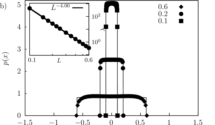
Figure 4: Stationary probability densities for different values of $L$ under rejection scheme. In the top panel (a)), the left part of the plot is presented in linear scale, while in the right part the semi-log scale is used. The bottom panel (b)) shows $\exp(-\lambda x^{4})$ fits and values of the fitted exponent $\lambda$ (inset).

The “rejection scheme” implicitly affects the jump length distribution and explicitly limits the accessible space to the $[-L,L]$ domain. Analogously like for the reflection scheme, we can expect that large enough boxes do not have the influence on modes positions, see Figs. 4 and 5. However, the critical box size is larger than for the “reflection scheme”. For $L\geqslant 5$ modes are located approximately at $\pm 1/\sqrt{2}$. Decreasing of $L$ below $L=5$ noticeably, although continuously, shifts locations of modal values toward $0$, see Figs. 4 and 5 showing histograms and modes locations for $V(x)=x^{4}/4$. Lastly, for sufficiently small $L$ the stationary density, under the “rejection scheme”, becomes unimodal. Fig. 6 shows the ratio of heights $\kappa_{h}$, see Eq. (9). Analogously, like in Fig. 3 the ratio of heights saturates for large $L$ at $\kappa_{h}=4/3$. However, in contrast to the “reflection scheme”, for small $L$, $\kappa_{h}$ tends to 1, because stationary densities with decreasing $L$ first become uniform around the origin, i.e., outer modes become weaker, and finally become unimodal.

Under “rejection scheme” the bimodality arises for large enough $L$, because a domain of motion is sufficiently large that a particle can reach a point which is distant enough to the origin from which the time of deterministic return to origin is infinite, see App. B. Consequently, a particle cannot return to the vicinity of the origin before the next jump to a distant point. For small $L$ the time of the deterministic return is still infinite but the diffusive spread compensates for it resulting in emergence of the unimodal stationary state. In other words, the diffusive spread is able to eradicate the minimum of the stationary density at the origin, which separates modes. Unfortunately, due to fluctuations of the histograms with small $L$ (especially around $x\approx 0$) it is hard to indicate the exact value of the transition point. Moreover, as demonstrated in Fig. 4b) stationary densities are practically of the truncated Boltzmann–Gibbs type, i.e., $p(x)\propto\exp[-\lambda V(x)]$ restricted to the $[-L,L]$ interval. The bottom part of Fig. 4 shows fitted densities (main plot) along with values of the fitted exponent $\lambda$ (inset) for the quartic potential. The truncated Boltzmann–Gibbs like densities are recorded for very small $L$ since rejection allows for very short jumps only, which mimics independence and limits spatial dependence among jumps. The fitted exponent $\lambda$ grows with the decrease in $L$, as for small $L$ stationary states are narrower.

Figure 5: The location of modes for the Cauchy noise for the quartic potential with different box sizes $[-L,L]$ under “rejection scheme”.

Figure 6: The ratio of heights $\kappa_{h}$, see Eq. (9), under the “rejection scheme”.

The “rejection scheme” can be interpreted as a random truncation scheme, as box edges introduce truncation of long jumps. Nevertheless, the level of truncation depends on the current position which determines the distance to the edge of the box and introduces the asymmetry to the effective jump length distribution. The typical (sharp) truncation scheme is studied in the next subsection.

III.3 Truncation scheme

In contrast to previously studied schemes, the “truncation scheme” does not limit the accessible space but directly cuts off the jump length distribution Mantegna and Stanley (1994). Only jumps for which $|\xi_{t}\Delta t^{1/\alpha}|<L$ are accepted, see Eq. (8). Therefore, the $\alpha$-stable distribution of stochastic parts of jumps is truncated to the $[-L,L]$ interval. For the “rejection setup”, constructed results are presented in a series of figures. Fig. 7 shows obtained histograms while Fig. 8 location of modes. Finally, Fig. 9 displays the relative height of modes.

At the first glance the rejection and truncation schemes bear some similarities, as both of them affect the jump length distribution. Nevertheless, they share fundamental differences which are mainly connected with the way how jumps are performed and how the accessible space is treated. Only under the “truncation scheme” random components of jumps are independent and identically distributed. In the “rejection scheme” a wandering particle cannot leave the $[-L,L]$ interval, while for the “truncation” it is possible. Moreover, under the “rejection scheme”, a particle located close to one of the boundaries can practically jump almost only in one (opposite) direction. Nevertheless, for $L<1$, the rejection does not result in accumulation of the probability mass in the vicinity of boundaries. In contrast, under the “truncation scheme”, the current position does not affect the jump length distribution The overall jump length is limited but the particle can reach a distant point from which it is efficiently returned to the neighborhood of the origin by the restoring force $-V^{\prime}(x)$. On the one hand, histograms for both setups are different, see Figs. 4 and 7. In particular, they differ with respect to the domain (finite interval versus real line), which determines the large $|x|$ dependence, and spread in the small $|x|$ range. In overall, on the other hand, despite these fundamental differences, dependence of the modes location is qualitatively the same under both scenarios, compare Fig. 5 and Fig. 8. Finally, Fig. 9 shows the ratio of heights $\kappa_{h}$ as a function of $L$, which again is very similar to the dependence observed for the “rejection scheme”. For large $L$, the ratio saturates at $\kappa_{h}=4/3$, while in the $L\to 0$ limits it tends to unity, because in the stationary states outer modes become weaker and finally disappear.

According to the central limit theorem Feller (1968); Gnedenko and Kolmogorov (1968) the sum of independent, identically distributed random variables characterized by a finite variance tends to the normal distribution. On the one hand, the $\alpha$-stable distribution is truncated, efficiently bounding independent random parts of jumps. On the other hand, we are studying the motion in the external potential, e.g., $V(x)=x^{4}/4$, for which subsequent displacements are not independent. Nevertheless, for sufficiently small $L$, i.e., $L\leqslant 0.6$, the stationary density is approximately given by the Boltzmann–Gibbs distribution, i.e., $p(x)\propto\exp[-\lambda V(x)]=\exp[-\lambda x^{4}]$, see bottom panel of Fig. 7. This effect can be intuitively explained. For small $L$ a particle does not easily explore distant points, thus it spends majority of time in the domain where the deterministic force (introducing dependence between jumps) is practically negligible. This results in the situation when jumps are approximately independent and identically distributed. Thanks to the central limit theorem the noise can be approximated by the Gaussian white noise and the emerging stationary density is of the Boltzmann–Gibbs type. The inset in Fig. 7b) displays fitted $\lambda$ as a function of the $L$. In contrast to small $L$, for large $L$ the deterministic nonlinear force introduces dependence between subsequent (long) jumps resulting in the violation of the central limit theorem and emergence of bimodal stationary states.

Figure 7: Stationary probability densities for different values of $L$ under the “truncation scheme”. The bottom panel (b)) shows normalized $\exp(-\lambda x^{4})$ curves fitted to numerically obtained histograms for small values of $L$, with the inset presenting dependence of $\lambda$ on $L$. In the top and bottom panels, the left part of the plot is presented in linear scale, while in the right part the semi-log scale is used.

Figure 8: The location of modes for the Cauchy noise and different box sizes $[-L,L]$ under the “truncation scheme”.

Figure 9: The ratio of heights $\kappa_{h}$, see Eq. (9), under the “truncation scheme”.

IV Summary and conclusions

The emergence of the multimodal stationary states under action of Lévy noises is determined by the combined action of Lévy flights and the deterministic force. In steeper than parabolic potential wells, stationary states are always (at least) bimodal, because the time of deterministic return to the origin diverges. Long excursions induced by Lévy flights cannot be compensated by the restoring force and diffusive spread, which is produced by the central part of the jump length distribution. Therefore, the stationary density attains the minimum at the origin.

In order to assess the role of long jumps in more detail we have studied several scenarios of limiting jump lengths. The numerical studies have shown that elimination of long jumps or truncation of jump length distribution can destroy bimodality, however a significant cutback is required. This indicates robustness of the bimodality in Lévy noise driven systems. Introduction of reflecting boundaries removes exploration of distant points but is not capable of destroying bimodality of a stationary state due to the nature of impenetrable boundaries which supports emergence of modes at edges. The accumulation of the probability mass at boundaries is especially strong for narrow intervals (centered at the origin) when the deterministic force is negligible.

We have assumed that long excursions are reduced by disregarding long jumps without any time penalty. On the operational level, jumps are drawn until one is drawn that satisfies the condition of constraints. Such a scenario corresponds to the so-called “accept-reject” method of generating (pseudo) random numbers Devroye (1986). Importantly, the obtained results will stay intact for a finite average penalty/waiting time in analogous way like the continuous time random walk scenarios with finite mean waiting time produce the Markovian diffusion Metzler and Klafter (2000) or finite return velocity does not change the non-equilibrium stationary state under stochastic resetting Evans and Majumdar (2011); Pal et al. (2019). More general types of waiting times, i.e., power-law distributed, will not change the shapes of stationary states but affects the way how these states are reached in a similar manner like subdiffusion does not affect stationary states Metzler and Klafter (2004) but only changes the way how they are approached.

Data availability

The data (generated randomly using the model presented in the paper) that supports the findings of this study is available from the corresponding author (PP) upon a reasonable request.

Appendixes

The additional information presenting information on $\alpha$-stable random variables, Lévy noise and deterministic sliding in a fixed potential is included in two appendices. This information is useful for examination of the stochastic system and understanding the origin of bimodality.

Appendix A $\alpha$-stable random variables and Lévy noise

The $\alpha$-stable noise is a generalization of the Gaussian white noise to the non-equilibrium realms Janicki and Weron (1994). The noise is still of the white type, i.e., it produces independent increments, but this time increments are distributed according to the heavy-tailed $\alpha$-stable density. Within the current manuscript, we restrict ourselves to symmetric $\alpha$-stable noise only, which is the formal time derivative of symmetric $\alpha$-stable process $L(t)$, see Refs. Janicki and Weron, 1994; Dubkov et al., 2008. Increments $\Delta L=L(t+\Delta t)-L(t)$ of the $\alpha$-stable process are independent and identically distributed according to an $\alpha$-stable density. Symmetric $\alpha$-stable densities are unimodal probability densities, with the characteristic function Samorodnitsky and Taqqu (1994); Janicki and Weron (1994)

$$\varphi(k)=\exp\left[-\sigma^{\alpha}|k|^{\alpha}\right].$$ (14)

The stability index $\alpha$ ($0<\alpha\leqslant 2$) determines the tail of the distribution, which for $\alpha<2$ is of the power-law type

$$p(x)\propto|x|^{-(\alpha+1)}.$$ (15)

The scale parameter $\sigma$ ($\sigma>0$) controls the width of the distribution, typically defined by an interquantile width or by fractional moments $\langle|x|^{\kappa}\rangle$ ($0<\kappa<\alpha$), because the variance of $\alpha$-stable variables diverges Samorodnitsky and Taqqu (1994); Weron and Weron (1995) for $\alpha<2$.

The characteristic function of the symmetric $\alpha$-stable density, see Eq. (14), reduces to the characteristic function of the normal distribution $N(0,2\sigma^{2})$ for $\alpha=2$,

$$f_{2}(x)=\frac{1}{\sqrt{4\pi\sigma^{2}}}\exp\left[-\frac{x^{2}}{4\sigma^{2}}\right],$$ (16)

while for $\alpha=1$ one gets the Cauchy distribution Janicki and Weron (1994)

$$f_{1}(x)=\frac{\sigma}{\pi}\frac{1}{\sigma^{2}+x^{2}}.$$ (17)

In other cases, $\alpha$-stable densities can be expressed using special functions Penson and Górska (2010); Górska and Penson (2011).

Appendix B Deterministic sliding

The Langevin equation

$$\dot{x}(t)=-V^{\prime}(x)+\xi(t)$$ (18)

in the zero noise limit for $V(x)=|x|^{c}/c$ ($c>0$) reduces to

$$\dot{x}(t)=-\mathrm{sign}(x)|x|^{c-1}.$$ (19)

From Eq. (19) one can find the dependence of $x(t)$ ($c\neq 2$)

$$x(t)=\left[x_{0}^{2-c}+(c-2)t\right]^{\frac{1}{2-c}},$$ (20)

while for $c=2$

$$x(t)=x_{0}\mathrm{e}^{-t}.$$ (21)

From $x(t)$ one can deduce that for any $x_{0}$ with $0<c<2$ the time of deterministic sliding to the origin is finite ($t=x_{0}^{2-c}/(2-c)$), while for $c\geqslant 2$ it diverges, because $\lim\limits_{t\to\infty}x(t)=0$. Therefore, the deterministic motion in power-law potential changes its properties at $c=2$. Moreover, the transition observed for $c>2$ plays an important role in noise driven systems as it is one of components required to induce bimodality of stationary states in single well potentials. More precisely, if the diffusive spread is unable to compensate for the diverging return time the stationary density becomes bimodal.

References

References

- Schimansky-Geier and Pöshel (1997) L. Schimansky-Geier and T. Pöshel, eds., Stochastic Dynamics (Springer Verlag, Berlin, 1997).
- Klafter et al. (2012) J. Klafter, S. T. Lim, and R. Metzler, Fractional dynamics: recent advances (World Scientific Publishing, Singapore, 2012).
- Tomé and De Oliveira (2016) T. Tomé and M. J. De Oliveira, Stochastic Dynamics and Irreversibility (Springer Verlag, Berlin, 2016).
- Gardiner (2009) C. W. Gardiner, Handbook of stochastic methods for physics, chemistry and natural sciences (Springer Verlag, Berlin, 2009).
- Risken (9996) H. Risken, The Fokker-Planck equation. Methods of solution and application (Springer Verlag, Berlin, 19996).
- Reichl (1998) L. E. Reichl, A modern course in statistical physics (John Wiley, New York, 1998).
- Chechkin et al. (2002a) A. V. Chechkin, J. Klafter, V. Y. Gonchar, R. Metzler, and L. V. Tanatarov, Chem. Phys. 284, 233 (2002a).
- Chechkin et al. (2003) A. V. Chechkin, J. Klafter, V. Y. Gonchar, R. Metzler, and L. V. Tanatarov, Phys. Rev. E 67, 010102(R) (2003).
- Cieśla et al. (2019) M. Cieśla, K. Capała, and B. Dybiec, Phys. Rev. E 99, 052118 (2019).
- Capała and Dybiec (2019) K. Capała and B. Dybiec, J. Stat. Mech. , 033206 (2019).
- Jacquet et al. (2018) Q. Jacquet, E.-j. Kim, and R. Hollerbach, Entropy 20, 613 (2018).
- Guggenberger et al. (2021) T. Guggenberger, A. Chechkin, and R. Metzler, J. Phys. A: Math. Theor. 54, 29LT01 (2021).
- Chechkin et al. (2006) A. V. Chechkin, V. Y. Gonchar, J. Klafter, and R. Metzler, in Fractals, Diffusion, and Relaxation in Disordered Complex Systems: Advances in Chemical Physics, Part B, Vol. 133, edited by W. T. Coffey and Y. P. Kalmykov (John Wiley & Sons, New York, 2006) pp. 439–496.
- Chechkin et al. (2008) A. V. Chechkin, R. Metzler, J. Klafter, and V. Y. Gonchar, in Anomalous transport: Foundations and applications, edited by R. Klages, G. Radons, and I. M. Sokolov (Wiley-VCH, Weinheim, 2008) pp. 129–162.
- Dubkov et al. (2008) A. A. Dubkov, B. Spagnolo, and V. V. Uchaikin, Int. J. Bifurcation Chaos. Appl. Sci. Eng. 18, 2649 (2008).
- Dybiec and Gudowska-Nowak (2009) B. Dybiec and E. Gudowska-Nowak, J. Stat. Mech. , 05004 (2009).
- Solomon et al. (1993) T. H. Solomon, E. R. Weeks, and H. L. Swinney, Phys. Rev. Lett. 71, 3975 (1993).
- Solomon et al. (1994) T. H. Solomon, E. R. Weeks, and H. L. Swinney, Physica D 76, 70 (1994).
- del Castillo-Negrete (1998) D. del Castillo-Negrete, Phys. Fluids 10, 576 (1998).
- Shlesinger et al. (1993) M. F. Shlesinger, G. M. Zaslavski, and J. Klafter, Nature (London) 363, 31 (1993).
- Klafter et al. (1996) J. Klafter, M. F. Shlesinger, and G. Zumofen, Phys. Today 49, 33 (1996).
- Chechkin et al. (2002b) A. V. Chechkin, V. Y. Gonchar, and M. Szydłowski, Phys. Plasmas 9, 78 (2002b).
- del Castillo-Negrete et al. (2005) D. del Castillo-Negrete, B. A. Carreras, and V. E. Lynch, Phys. Rev. Lett. 94, 065003 (2005).
- Katori et al. (1997) H. Katori, S. Schlipf, and H. Walther, Phys. Rev. Lett. 79, 2221 (1997).
- Peng et al. (1993) C.-K. Peng, J. Mietus, J. M. Hausdorff, S. Havlin, H. E. Stanley, and A. L. Goldberger, Phys. Rev. Lett. 70, 1343 (1993).
- Segev et al. (2002) R. Segev, M. Benveniste, E. Hulata, N. Cohen, A. Palevski, E. Kapon, Y. Shapira, and E. Ben-Jacob, Phys. Rev. Lett. 88, 118102 (2002).
- Lomholt et al. (2005) M. A. Lomholt, T. Ambjörnsson, and R. Metzler, Phys. Rev. Lett. 95, 260603 (2005).
- Viswanathan et al. (1996) G. M. Viswanathan, V. Afanasyev, S. V. Buldyrev, E. J. Murphy, P. A. Prince, and H. E. Stanley, Nature (London) 381, 413 (1996).
- Brockmann et al. (2006) D. Brockmann, L. Hufnagel, and T. Geisel, Nature (London) 439, 462 (2006).
- Evans and Majumdar (2011) M. R. Evans and S. N. Majumdar, Phys Rev. Lett. 106, 160601 (2011).
- Evans et al. (2020) M. R. Evans, S. N. Majumdar, and G. Schehr, J. Phys. A: Math. Theor. 53, 193001 (2020).
- Gupta and Jayannavar (2022) S. Gupta and A. M. Jayannavar, Front. Phys. , 10:789097 (2022).
- Janicki and Weron (1994) A. Janicki and A. Weron, Simulation and chaotic behavior of -stable stochastic processes (Marcel Dekker, New York, 1994).
- Ditlevsen (1999) P. D. Ditlevsen, Geophys. Res. Lett. 26, 1441 (1999).
- Mercadier et al. (2009) M. Mercadier, W. Guerin, M. M. Chevrollier, and R. Kaiser, Nat. Phys. 5, 602 (2009).
- Barkai et al. (2014) E. Barkai, E. Aghion, and D. A. Kessler, Phys. Rev. X 4, 021036 (2014).
- Amor et al. (2016) T. A. Amor, S. D. S. Reis, D. Campos, H. J. Herrmann, and J. S. Andrade, Sci. Rep. 6, 20815 (2016).
- Barthelemy et al. (2008) P. Barthelemy, J. Bertolotti, and D. Wiersma, Nature (London) 453, 495 (2008).
- Fioriti et al. (2015) V. Fioriti, F. Fratichini, S. Chiesa, and C. Moriconi, Int. J. Adv. Robot. Syst. 12, 98 (2015).
- Lera and Sornette (2018) S. C. Lera and D. Sornette, Phys. Rev. E 97, 012150 (2018).
- Samorodnitsky and Taqqu (1994) G. Samorodnitsky and M. S. Taqqu, Stable non-Gaussian random processes: Stochastic models with infinite variance (Chapman and Hall, New York, 1994).
- Jespersen et al. (1999) S. Jespersen, R. Metzler, and H. C. Fogedby, Phys. Rev. E 59, 2736 (1999).
- Yanovsky et al. (2000) V. V. Yanovsky, A. V. Chechkin, D. Schertzer, and A. V. Tur, Physica A 282, 13 (2000).
- Schertzer et al. (2001) D. Schertzer, M. Larchevêque, J. Duan, V. V. Yanovsky, and S. Lovejoy, J. Math. Phys. 42, 200 (2001).
- Podlubny (1999) I. Podlubny, Fractional differential equations (Academic Press, San Diego, 1999).
- Samko et al. (1993) S. G. Samko, A. A. Kilbas, and O. I. Marichev, Fractional integrals and derivatives. Theory and applications. (Gordon and Breach Science Publishers, Yverdon, 1993).
- Padash et al. (2019) A. Padash, A. V. Chechkin, B. Dybiec, I. Pavlyukevich, B. Shokri, and R. Metzler, J. Phys. A: Math. Theor. 52, 454004 (2019).
- Kwaśnicki (2017) M. Kwaśnicki, Fractional Calculus Appl. Anal. 20, 7 (2017).
- Song et al. (2017) F. Song, C. Xu, and G. E. Karniadakis, SIAM J. Sci. Comput. 39, A1320 (2017).
- Cusimano et al. (2018) N. Cusimano, F. del Teso, L. Gerardo-Giorda, and G. Pagnini, SIAM J. Numer. Anal. 56, 1243 (2018).
- Chechkin et al. (2004) A. V. Chechkin, V. Y. Gonchar, J. Klafter, R. Metzler, and L. V. Tanatarov, J. Stat. Phys. 115, 1505 (2004).
- Dybiec et al. (2010) B. Dybiec, A. V. Chechkin, and I. M. Sokolov, J. Stat. Mech. , P07008 (2010).
- Dybiec et al. (2007) B. Dybiec, E. Gudowska-Nowak, and I. M. Sokolov, Phys. Rev. E 76, 041122 (2007).
- Dubkov and Spagnolo (2007) A. A. Dubkov and B. Spagnolo, Acta Phys. Pol. B 38, 1745 (2007).
- Denisov et al. (2008) S. I. Denisov, W. Horsthemke, and P. Hänggi, Phys. Rev. E 77, 061112 (2008).
- Dybiec et al. (2017) B. Dybiec, E. Gudowska-Nowak, E. Barkai, and A. A. Dubkov, Phys. Rev. E 95, 052102 (2017).
- Higham (2001) D. J. Higham, SIAM Review 43, 525 (2001).
- Mannella (2002) R. Mannella, Int. J. Mod. Phys. C 13, 1177 (2002).
- Chambers et al. (1976) J. M. Chambers, C. L. Mallows, and B. W. Stuck, J. Am. Stat. Assoc. 71, 340 (1976).
- Weron (1996) R. Weron, Statist. Probab. Lett. 28, 165 (1996).
- Devroye (1986) L. Devroye, Non-uniform random variate generation (Springer Verlag, New York, 1986).
- Newman and Barkema (1999) M. E. J. Newman and G. T. Barkema, Monte Carlo methods in statistical physics (Oxford University Press, Oxford, 1999).
- Kharcheva et al. (2016) A. A. Kharcheva, A. A. Dubkov, B. Dybiec, B. Spagnolo, and D. Valenti, J. Stat. Mech. 2016, P054039 (2016).
- Mantegna and Stanley (1994) R. N. Mantegna and H. E. Stanley, Phys. Rev. Lett. 73, 2946 (1994).
- Feller (1968) W. Feller, An introduction to probability theory and its applications (John Wiley, New York, 1968).
- Gnedenko and Kolmogorov (1968) B. V. Gnedenko and A. N. Kolmogorov, Limit distributions for sums of independent random variables (Addison–Wesley, Reading, MA, 1968).
- Metzler and Klafter (2000) R. Metzler and J. Klafter, Phys. Rep. 339, 1 (2000).
- Pal et al. (2019) A. Pal, Ł. Kuśmierz, and S. Reuveni, Phys. Rev. E 100, 040101 (2019).
- Metzler and Klafter (2004) R. Metzler and J. Klafter, J. Phys. A: Math. Gen. 37, R161 (2004).
- Weron and Weron (1995) A. Weron and R. Weron, Lect. Not. Phys. 457, 379 (1995).
- Penson and Górska (2010) K. A. Penson and K. Górska, Phys. Rev. Lett. 105, 210604 (2010).
- Górska and Penson (2011) K. Górska and K. A. Penson, Phys. Rev. E 83, 061125 (2011).