Impact of (magneto-)thermoelectric effect on diffusion of conserved charges in hot and dense hadronic matter
Abstract
We investigate the thermoelectric effect, which describes the 5generation of an electric field induced by temperature and conserved charge chemical potential gradients, in the hot and dense hadronic matter created in heavy-ion collisions. Utilizing the Boltzmann kinetic theory within the repulsive mean-field hadron resonance gas model, we evaluate both the diffusion thermopower matrix and diffusion coefficient matrix for the baryon number (), electric charge (), and strangeness ().The Landau-Lifshitz frame is enforced in the derivation. We find that the thermoelectric effect hinders the diffusion processes of multiple conserved charges, particularly reducing the coupling between electric charge and baryon number (strangeness) in baryon (strangeness) diffusion. Based on the fact that the repulsive mean-field interactions between hadrons have a significant effect on the diffusion thermopower matrix and diffusion coefficient matrix in the baryon-rich region, we extend the investigation to include the impact of the magnetic field, analyzing the magneto-thermoelectric effect on both the diffusion coefficient matrix and the Hall-like diffusion coefficient matrix. The sensitivity of the magnetic field-dependent diffusion thermopower matrix and magneto-thermoelectric modified diffusion coefficient matrix to the choices of various transverse conditions is also studied.
I Introduction
Relativistic heavy-ion collision experiments open up a unique portal for understanding the properties of strongly interacting matter under extreme temperatures. A lot of experimental evidence in the relativistic heavy-ion collider (RHIC) BRAHMS:2004adc ; PHOBOS:2004zne ; PHENIX:2004vcz ; STAR:2005gfr at Brookhaven National Laboratory (BNL) and in the large hadron collider (LHC) ALICE:2010khr ; CMS:2011aqh ; CMS:2011iwn ; CMS:2012xss ; ATLAS:2011ah ; ALICE:2010yje at the European Organization for Nuclear Research (CERN) have indicated that a new deconfined state of matter – quark-gluon plasma (QGP) can be created. On the other hand, quantum chromodynamics (QCD) is the fundamental theory of the strong interaction and the lattice QCD calculation has predicted a smooth crossover for QCD matter from a hadronic phase to a QGP phase can be realized with increasing temperature () at the small or vanishing baryon chemical potential () Aoki:2006we ; Cheng:2006qk ; Philipsen:2012nu . At large , the calculations in the low energy QCD effective models, viz., the (Polyakov-loop-) Nambu-Jona-Lasinio model Nambu:1961tp ; Hatsuda:1994pi ; Fukushima:2008wg , the (Polyakov-loop-) quark-meson model Schaefer:2006ds ; Schaefer:2007pw ; Schaefer:2008hk ; Schaefer:2011ex have indicated that the QCD phase transition becomes a first-order phase transition and terminates at the critical endpoint (CEP) of second-order, which has sparked long-sought debate without conclusive experimental evidence yet Lacey:2014wqa . Besides, the Beam Energy Scan (BES) program at RHIC STAR:2010vob ; Mohanty:2011nm and ongoing experimental programs at Facility for Antiproton and Ion Research (FAIR) Tahir:2005zz ; CBM:2016kpk and Nuclotron-based Ion Collider fAcility (NICA) Friman ; Kekelidze:2012zz also endeavor to shed light on the properties of dense nuclear matter and search the potential signature of the CEP in the QCD phase diagram.
Besides the equilibrium QCD thermodynamic properties, the medium response to perturbation around equilibrium, characterized by transport coefficients, plays an important role in describing the dynamics of bulk matter created in relativistic heavy-ion collisions. The ratio of shear viscosity to entropy density () has been shown to give a good description of flow data Romatschke:2007mq ; Kovtun:2004de ; Heinz:2013th . The bulk viscosity to entropy density () exhibits a novel behavior at some characteristic temperatures Sasaki:2008fg ; Karsch:2007jc . During recent research Roy:2015kma ; Roy:2017yvg , electric conductivity has also been used as an input in magneto-hydrodynamic simulations of heavy-ion collisions. On the other hand, the diffusion coefficient, which describes the medium response to inhomogeneities in the number density and almost is ignored at top RHIC and LHC energies, becomes significant in low-energy heavy-ion collisions. Typically the diffusion coefficient matrix, measuring the coupling among diffusion currents of different conserved charges of the system, is required to give a proper dynamical description of low-energy heavy-ion collisions. This results from the fact that QCD matter constituents (hadrons and quarks) carry multiple quantum conserved numbers, e.g., baryon number (), electric charge (), strangeness (), etc. The complete diffusion coefficient matrix in both the QGP and hadron gas has been calculated within the Boltzmann kinetic theory Greif:2017byw ; Fotakis:2019nbq ; Fotakis:2021diq and the results reveal that the off-diagonal matrix elements in magnitude share the same order with diagonal ones and cannot be neglected in the hydrodynamic simulation of low-energy nuclear collisions. Recently, A. Das et. al. have explicitly imposed the Landau-Lifshitz frame into the previous derivation in Greif:2017byw ; Fotakis:2019nbq and provide a unique expression in the hadron resonance gas model with and without excluded volume corrections Das:2021bkz . In this work, we explore the effect of repulsive interactions on the diffusion properties of hadronic matter in the repulsive mean-field hadron resonance gas (RMFHRG) model, where the repulsive interactions between hadrons are considered through a density-dependent mean-field potential, and subsequently modify the diffusion coefficient.
The thermoelectric effect, a phenomenon involving the direct conversion of temperature differences to electric voltage and vice versa, has been extensively explored across various disciplines such as material science, solid-state physics, and chemistry. A well-known thermoelectric effect is the Seebeck effect, which refers to the generation of electric voltage caused by a temperature gradient in a semiconductor or conductor. Heavy-ion collisions allow us to study the Seebeck effect of QCD matter due to the temperature difference between the central region and peripheral region of the fireball. The Seebeck coefficient, defined as the ratio of the induced electric field and the collinear temperature gradient () in the absence of electric current, has been estimated in both the partonic and hadron phase of QCD matter Zhang:2020efz ; Das:2021qii ; Zhang:2021xib ; Kurian:2021zyb ; Dey:2020sbm ; Dey:2021crc ; Khan:2022apd ; Bhatt:2018ncr ; Das:2020beh . Differing from the condensed matter studies, the non-vanishing net conserved number is required for the estimation of the Seebeck coefficient in QCD matter. To our best knowledge, all estimations are performed when only net baryon density is nonzero, without taking into account the contribution of other conserved charges to the thermoelectric effect. Actually, the gradients of multiple conserved charge chemical thermal potentials with also is a source to generate an internal electric field, which is quantified by diffusion thermopower matrix in the limit of zero electric current. Such thermoelectric effect involving multiple conserved charges might further affect the recently proposed thermally spin Hall effect (TSHE) in the heavy-ion collisions at BES energies Liu:2020dxg ; Fu:2022myl . As the thermoelectric effect is highly related to the gradient of conserved charge chemical potential, and it can affect the diffusion coefficient matrix in principle, to the best of our knowledge, there are no associated studies yet, which is the main motivation for our research.
Considering that a partial magnetic field created in the off-central heavy-ion collisions can survive to the hadronic phase due to the electric conductivity of medium Voronyuk:2011jd ; Tuchin:2010gx ; McLerran:2013hla , the motions of charged hadron driven by can be deflected. This results in the generation of a transverse or Hall-like electric field, viz, in the magnetic field, known as the magneto-thermoelectric effect, which is measure by Hall-like diffusion thermopower. Similarly, the extra Hall-type diffusion currents of conserved charges also appear in the magnetic field and are quantified by the Hall-like diffusion coefficient matrix. The magneto-thermoelectric effect can affect both the diffusion coefficient matrix and the Hall-like diffusion coefficient matrix. Importantly, the expression of the magneto-thermoelectric modified diffusion coefficient matrix depends on the choices of transverse conditions: (1) all transverse gradients in temperature and chemical potential of conserved charge vanishes; (2) other transverse specific conserved charge diffusion current disappears apart from vanishing transverse electric current.
This paper is organized as follows. In Sec. II, we give a brief overview of the ideal hadron resonance gas (IHRG) model and repulsive mean-field hadron resonance gas (RMFHRG) model. The general expression for the diffusion thermopower and diffusion coefficient of conserved charges will be derived in Sec. III by solving the Boltzmann equation under relaxation time approximation in the framework of the RMFHRG model with and without magnetic field. We for the first time present the formulas of magneto-thermoelectric modified diffusion coefficient matrix under different transverse conditions. Sec. IV will discuss the influences of RMF correction, baryon chemical potential, magnetic field, and (magneto-)thermoelectric effect on the (Hall-like-) diffusion coefficient matrix. Finally comes our summary of this work in Sec. V.
Throughout this paper we adopt natural units , and work in flat Minkowski space-time with metric tensor thus the fluid velocity satisfies . is the projection operator onto the three-dimensional subspace orthogonal to , . The projection of any four-vector onto the three-dimensional subspace orthogonal to as . The four-derivative can be decomposed as , and denote the time derivative and spatial gradient operator in the local rest frame, respectively. In the local rest frame , .
II Model description
Hadron resonance gas (HRG) model Cleymans:1999st ; Becattini:2000jw is a simplistic thermal statistical model that successfully describes the low-temperature hadronic phase of QCD at chemical freeze-out. In the IHRG model, the attractive interactions between hadrons are implicitly considered by including all the resonances with zero width, while the repulsive interactions among hadrons, which are already known from nucleon-nucleon scattering experiments, are missing in the IHRG model. Accordingly, the extended versions of the IHRG model e.g., excluded volume HRG model Rischke:1991ke ; Andronic:2012ut ; Kadam:2015xsa , van der Waals HRG model Vovchenko:2016rkn ; Vovchenko:2017zpj and repulsive mean-field HRG model Pal:2023zzp ; Huovinen:2017ogf ; Kadam:2019peo ; Pal:2020ucy , are proposed to give a better fitting to various thermodynamic observables obtained from lattice QCD. In this work, the repulsive interactions between the hadrons are incorporated via a mean-field approach, and this extended version of the IHRG model is the so-called repulsive mean-field hadron resonance gas (RMFHRG) model.
II.1 Ideal hadron resonance gas (IHRG) model
In the IHRG model, the partition function containing all relevant degrees of freedom of the confined QCD phase is the starting point for obtaining the thermodynamics. The logarithm of the total partition function in the grand canonical ensemble is given as
| (1) |
where the partition function of hadron species is
| (2) |
Here, the superscript presents to the ideal gas and is the system volume, we use the notation , is the spin degeneracy of hadron species . is the inverse temperature of the system. The front upper (lower) sign corresponds to fermions (bosons). is the single particle energy with mass . is the chemical potential of species , where , with , , being baryon, electric and strangeness chemical potential, respectively, , and are the baryon number, electric charge, and strangeness of the respective particle species . Accordingly, the ideal thermodynamics such as total pressure , total energy density , and total number density in the IHRG model can be obtained as:
| (3) | |||||
| (4) | |||||
| (5) |
Here, is the thermal equilibrium distribution function of particle species in the IHRG model, which is given as
| (6) |
where the refers to the Fermi-Dirac and Bose-Einstein distribution functions, respectively.
II.2 Repulsive mean-field hadron resonance gas (RMFHRG) model
The RMFHRG model is a minimal extension of the IHRG model by including short-range repulsive interactions between hadrons via a mean-field approach, where the single-particle energy gets modified as Olive:1980dy
| (7) |
where is the potential describing the repulsive interactions between hadrons and also behaves as the effective chemical potential. In this model, only the repulsive interactions among meson-meson pairs, baryon-baryon pairs, and antibaryon-antibaryon pairs are accounted Kadam:2019peo . Then the mean-field potentials for (anti-)baryons and mesons are given as Olive:1980dy ; Kadam:2019peo
| (8) |
where the subscripts , denote baryons, antibaryons, and mesons, respectively, are the associated total baryon, antibaryon, and meson number densities, respectively. Two phenomenological parameters and are introduced to scale the repulsive interaction strength among the mesons and (anti-)baryons, respectively. Accordingly, the logarithm of total partition function in the RMFHRG model is written as
| (9) | |||||
where the effective chemical potential is for (anti-)baryons, and for mesons. In the RMFHRG model, have following form:
| (10) |
Here, is the thermal equilibrium distribution function of particle species in the RMFHRG model, which reads as
| (11) |
In Eq. (9), is an additional correction factor to avoid the double counting of the mean-field potential and renders the correct number density per particle (or the correct energy density per particle ), assuming hadron species is a baryon or antibaryon, we can get
| (12) |
Hence, we can get the following form of :
| (13) |
If hadron species is a meson, . Using Eqs. (3-4) as well as Eq. (9), we can get the pressure and energy density for baryons, antibaryons, and mesons in the RMFHRG model, which are expressed respectively as
| (14) | |||||
| (15) |
The total pressure and total energy density in the RMFHRG model are and , respectively. It’s seen that the RMFHRG model gives an additional term in pressure and energy density compared to the IHRG model, the thermodynamic relation is still consistently satisfied. In the present RMFHRG model, all different (anti-)baryons or mesons have the same repulsive interaction strength, and are used to improve the agreement with the thermodynamic quantities obtained from the lattice QCD simulations at zero and finite baryon density Kadam:2019peo ; Pal:2020ucy .
III Thermoelectric coefficients and diffusion coefficients of conserved charges in Boltzmann kinetic theory
III.1 formalism
It is effective to calculate the transport coefficients of hadronic matter within the framework of the kinetic theory. The evolution of the single-particle phase-space distribution function can be described by the Boltzmann equation within the covariant formalism SMASH:2016zqf ,
| (16) |
where is the four-momentum of the particle species , is the four-force experienced by individual particle, as well as represents the collision term. When the particle is affected by electromagnetic field force, then , with being the repulsive mean-field potential among hadrons; is the electromagnetic field-strength tensor, , with being the totally anti-symmetric Levi-Civita tensor. The four-vectors and are nothing but the electric and magnetic fields measured in the frame where the fluid moves with a velocity . and are all space like, , and can be normalized as , where and . Note that in this work the electric field is induced by gradients of conserved charge density rather than an external field.
Considering that the system is slightly deviated from the local equilibrium, then the phase space distribution function of species has the following form:
| (17) |
where the deviation function is . is the local equilibrium distribution function in the RMFHRG model,
| (18) |
Here, is defined as the chemical thermal potential of conserved charge .
To get the solution to Eq. (16), the deviation function must have the following linear combination form:
| (19) |
where and are unknown functions with momentum . Considering the scattering process only for the sake of simplicity, the collision term in Eq. (16) is given as Chakraborty:2010fr ; Albright:2015fpa
| (20) |
where for bosons and fermions, respectively. is the collisional transition rate. The factor takes into account the possibility that the incoming particles are identical. Using the detailed balance condition , the collision term can be rewritten as
| (21) | |||||
Here, we have assumed particle species is out of equilibrium (), while all other particles are in equilibrium (). On the other hand, we shall consider the collision term of Eq. (16) in a simple and popular approximation called the relaxation time approximation (RTA) Anderson , then the collision term can be simplified as:
| (22) |
Here, is the relaxation time of species which describes how fast the system reaches the equilibrium again. is perturbation term. Then, the energy-momentum tensor and the net conserved charge four-current can be expressed in terms of the phase space distribution function as follows:
| (23) | |||||
| (24) |
with . In the non-equilibrium system, the energy-momentum diffusion four-current and the conserved charge diffusion four-current are and , respectively Fotakis:2022usk ; Molnar:2016vvu , which also can be written as
| (25) | ||||
| (26) |
Unlike the ideal hydrodynamics in which the fluid four-velocity is determined because the energy and conserved charge number current flowing parallel to each other, and then the local rest frame of fluid is defined via the requirement that these currents vanish identically, the energy flow and charge number flow in the dissipative hydrodynamics are separate, then the definition of fluid four-velocity is not uniquely defined DerradideSouza:2015kpt . There are two simple and natural choices to fix the local rest frame of fluid, i.e., Eckart (or conserved charge) frame and Landau-Lifshitz (or energy) frame. In the Eckart frame, the fluid velocity is parallel to one of the conserved charge currents, and the overall diffusion of one of the conserved net charges vanishes in the local rest frame. However, in low-energy heavy-ion collisions, there are multiple conserved charges, which are not necessarily non-vanishing in all regions of space-time, the definition of the rest frame according to Eckart is less suitable Fotakis:2022usk . In the Landau-Lifshitz frame, the fluid velocity is parallel to the energy flow, and the energy diffusion current in the local rest frame is required to vanish. In the present study, the Landau-Lifshitz matching condition in the local rest frame is imposed during the derivation of transport coefficients.
Replacing the right-hand side of Eq. (16) with Eq. (22), the perturbation term for the first-order gradient expansion is computed as
| (27) | |||||
where , the rank-two tensor leading to . In the ideal hydrodynamics, taking the projection of in the direction orthogonal to , one gets , where the is expansion rate. Since , we have , then we can get with being enthalpy density. Recalling the Gibbs-Duhem relation: , one obtains with being conserved net charge density. Using momentum conservation , we can get .
III.2 for vanishing magnetic field
In Eq. (27), we first only consider spatial-dependent gradient terms, and don’t consider magnetic field effect, then can be reduced as
| (28) | |||||
Only keep the terms related to the conserved charge diffusion current, above equation is again reduced as
| (29) |
The functions of and in Eq. (29) are given as
| (30) | |||||
| (31) |
In the Landau-Lishift matching condition, the energy flow is required to vanish in the local rest frame of fluid, i.e., , then inserting Eq. (19) into Eq. (25), one gets
| (32) |
Considering that we have the particular solutions , , another solutions can be written as and , respectively, where and are the constant independent of particle species . Then inserting these into Eq. (32) to resolve the freedom of solutions, we can get
| (33) | |||||
Using the identity , and comparing the coefficients of and , we can get
| (34) | |||||
| (35) |
Inserting Eq. (19) into Eq. (26), and using Eqs. (34-35) as well as the identity , the diffusion current of conserved charge can be written as
| (36) | |||||
We replace the right-hand side of Eq. (22) using Eq. (29), and substitute with Eq. (19) into the left-hand side of Eq. (22), then equate and by matching tensor structure, the particular solutions for the functions and from finally are computed as:
| (37) | |||||
| (38) |
According to the linear response theory, Eq. (36) can be presented as the following matrix form:
| (39) |
Here, the diffusion coefficient matrix (), which quantifies the coupling between the diffusion of different conserved charges, reads as
| (40) | |||||
which is equivalent to the expression derived from Ref. Das:2021bkz , if ignoring the effect of quantum statistics and the repulsive mean-field interactions between hadrons. In Eq. (39), the thermoelectric transport coefficient matrix is given as
| (41) | |||||
Take , the is redefined as thermoelectric conductivity of conserved charge . When net electric diffusion current vanishes, i.e., , we can get the induced internal electric field:
| (42) |
Here, is defined as diffusion thermopower of conserved charge , which quantifies the ability of hadronic matter to convert the gradients of conserved charge chemical thermal potential to an electric field, and it reads as
| (43) |
Inserting Eq. (42) into Eq. (39), then the matrix form of Eq. (36) can be rewritten as
| (44) |
Here, the thermoelectric modified diffusion coefficients in the electric current sector vanish, i.e., . The thermoelectric modified diffusion coefficient matrix elements in baryon and strangeness sectors have the following form:
| (45) |
with .
III.3 for finite magnetic field
Next, we investigate the influence of the magnetic field on the thermoelectric effect and diffusion processes of multiple conserved charges in the hadronic medium. In the presence of a weak magnetic field, the magnetic field is not the dominant energy scale and its impact can be manifested at the classical level with the so-called cyclotron motion of charged particles. We reasonably propose that the scattering mechanism of constituents and the thermodynamic quantities are unaffected by the magnetic field. In the uniform electric field and external magnetic field (), considering a time-independent phase space distribution function, Eq. (16) can be reformulated as
| (46) |
where the RTA has been utilized, and is the three-velocity of particle species . Neglecting any term that is second order in , Eq. (46) can be rewritten as
| (47) | |||||
We further assume the solution of Eq. (47) satisfies the following linear form,
| (48) | |||||
with being an unknown quantity related to the magnetic field. Inserting Eq. (48) into Eq. (47) we obtain
| (49) | |||||
After some tedious calculations, we can get the form as follows:
| (50) | |||||
where , all the information of magnetic field is encoded in cyclotron frequency of species , i.e., . Inserting Eq. (50) into Eq. (48), we finally obtain the magnetic field-dependent perturbation term of the distribution function,
| (51) | |||||
Repeating some procedures in the previous subsection (Eqs. (17)-(26), Eqs. (32)-(38)), the particular solutions for the functions and from in the magnetic field are computed as
| (52) | |||||
| (53) |
Therefore, the diffusion current of conserved charge in the magnetic field is computed as:
| (54) | |||||
Take the magnetic field along the -axis and decompose the above equation into - and -directions, the following matrix form can be obtained:
| (55) |
Here, the thermoelectric conductivity tensors () and diffusion coefficient tensors () in a magnetic field satisfy the Onsager’s reciprocity relation Callen ; Redin : and . Accordingly, the magnetic field-dependent thermoelectric conductivity matrix element () and the Hall-like or transverse thermoelectric conductivity matrix element () can be expressed as
| (56) | |||||
The magnetic field-dependent diffusion coefficient matrix element () and the Hall-like diffusion coefficient matrix element () can be given as
| (57) | |||||
To better distinguish the expressions of transport coefficients in different transverse restriction conditions later, we convert Eq. (55) into the following matrix form:
| (58) |
Solving the set of coupled matrix equations (58) under the condition of vanishing gradients of transverse conserved charge chemical thermal potential () with , then the electric resistance tensors () can be obtained as
| (59) | |||||
| (60) |
Similarly, a Hall-like diffusion thermopower of conserved charge () can appear in the magnetic field. Under the condition of with , the magnetic field-dependent diffusion thermopower and Hall-like diffusion thermopower of conserved charge can respectively be obtained as
| (61) | ||||
| (62) |
Taking vanishing magnetic field, . Using the set of coupled equations (58), the magneto-thermoelectric modified diffusion coefficient () and Hall-like magneto-thermoelectric modified diffusion coefficient () under the condition of with , can respectively be computed as
| (63) | |||||
| (64) | |||||
In condensed matter physics, a transverse temperature gradient () can be developed by the longitudinal temperature gradient () under a static magnetic field (), which is called the Righi-Leduc effect or thermal Hall effect. The associated Righi-Leduc coefficient is calculated in the transverse adiabatic condition i.e., , with being transverse heat current. In the hadronic matter with multiple conserved charges, similar to the Righi-Leduc effect, a transverse or Hall-like conserved charge density gradient () perpendicular to both the and can be generated. The corresponding coefficient is obtained under the condition of vanishing transverse diffusion current i.e., . Hence, using the matrix Eq. (58), and imposing the conditions of , the Righi-Leduc-type relation in the hadronic medium reads as
| (65) | |||||
with being Righi-Leduc-like coefficient. Accordingly, the magnetic field-dependent diffusion thermopower under the condition of with is computed as
| (66) |
When the magnetic field is turned off, the expressions of transport coefficients in the transverse condition of equal to those in the transverse condition of . Similarly, the magneto-thermoelectric modified diffusion coefficient under the condition of with , is computed as
| (67) |
III.4 Thermal averaged relaxation time
Comparing Eq. (21) and Eq. (22), all the scattering information of hadrons is encoded in the relaxation time, , and its inverse is given as
| (68) | |||||
The collisional transition rate is given as
| (69) |
where is the dimensionless transition amplitude averaged over the spin degeneracy factor in both initial and final states. To simplify the estimation of relaxation time, , and we use the formula of scattering cross section Peskin:1995ev
| (70) |
then we can rewrite as
| (71) |
where is the number density of species . It’s worth noting the RMF interactions between hadrons can enter the scattering process by modifying the number density of hadron species , hence the number density of hadron species needs to be distinguished in the IHRG model and RMFHRG models. In Eq. (71), the relative velocity is defined as
| (72) |
In this work, we shall consider the momentum-independent relaxation time, then thermal averaged cross section can be given as
| (73) |
We only consider elastic scattering for the 2-to-2 process and all hadrons are regarded as hard spheres with the same radius and is a constant with mb.
IV numerical results and discussions
IV.1 Results for vanishing magnetic field
All our calculations are performed in the condition of Fotakis:2019nbq ; Das:2021bkz , which is expected in the initial stages of heavy-ion collision Cleymans:1992zc ; Greiner:1987tg . This results in a nonzero strangeness chemical potential, which is a function of and . In the HRG models, we take all available hadrons up to a mass cutoff GeV from available Thermal-FIST package Vovchenko:2019pjl . The BES program at RHIC covers beam energy from GeV to 200 GeV, with the baryon chemical potential ranging from GeV to 0.02 GeV Cleymans:2005xv ; Odyniec:2013kna ; STAR:2022vlo , we take GeV in this investigation. To better understand the behaviors of the diffusion coefficient matrix later, we first detailedly discuss the and dependence of the scaled conductivity matrix , which is given as
| (74) |
It is highly related to diffusion coefficient matrix and is equal to at . Actually, the variation of with and is determined by the interplay between charge number density (or distribution function) and scattering rate (or the relaxation time ).
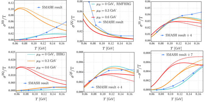
In Fig. 1, we see that for , the () in magnitude decreases (increases) monotonically as increases, whereas both and first increase with and then decrease, which is qualitatively consistent with the SMASH simulation results (symbol lines) Hammelmann:2023fqw The sign of is negative due to the associated dominant carriers, viz hyperons carrying a positive baryon number with a negative strangeness. As shown in Fig. 1, all scaled conductivities in the SMASH simulation with Green-Kubo formalism are larger than our results. We can also see that the effect of RMF interaction on the conductivity matrix for is minimal. This is because the RMF correction for only has a small suppression on charge number density and a small enhancement on relaxation time, the mutual compensation makes the RMF correction on the conductivities ignorable.
The thermal behaviors of all scaled conductivities for GeV are almost unchanged compared to the case of , and from Fig. 1 we note that in magnitude has an obvious enhancement because the dependence of on is mainly governed by the baryon density, which is an increasing function of . We also observe that and at GeV have a nominal reduction compared to those at . The reason behind this is that the dominant carriers for both and are kaons (), the number density of kaons has a small enhancement due to the presence of nonzero , whereas such enhancement can be canceled out by the increase of the scattering rates of kaons due to colliding with more baryons. The also has an invisible variation at GeV compared at , which is the competition result between meson contribution (mostly pions) to and baryon contribution (mostly nucleons) to . At GeV, the decrease of pion contribution to with is almost compensated by the increase of nucleon contribution to with . As increases further, the baryon density becomes more and more significant, and all conductivities at GeV have a significant variation. We note that the temperature dependence of both and even can overturn at GeV. This is because the decreasing behavior of the relaxation time of predominant nucleons with dominates over the increasing behavior of the distribution function with . We also observe that all conductivities except have a significant variation due to the RMF correction at GeV compared to those at or 0.3 GeV. The , , and has an obvious suppression because the including of the RMF correction significantly decreases the baryon density of the system at GeV.
While the RMF correction leads a significant enhancement on and at GeV compared that at GeV. This is because at GeV the associated predominant carriers to both the and are still kaons, the kaon density only is affected by the RMF interaction between meson and meson, while the relaxation time of kaons can be influenced by the RMF interaction among various hadron-hadron pairs due to colliding with different hadrons, which are canceled out at GeV. As increases further, the increase in kaon relaxation time caused by the RMF correction significantly overtakes the decrease in the kaon density, leading to a visible enhancement on both and at GeV. For purely electric conductivity , it nearly cannot be changed by the RMF correction even at high . The reason behind this just is the exact cancellation between the RMF correction on the contributed by mesons and the RMF correction on the contributed by baryons. The and dependence of all conductivities can not be altered by adding the RMF interactions.
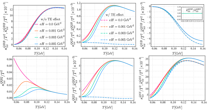
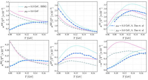
With the knowledge provided above, we can easily comprehend the results of the diffusion coefficient matrix. In Fig. 2, we display the and dependence of complete scaled diffusion coefficient matrix in both the IHRG and RMFHRG models. Similar to the conductivity matrix, the and are symmetric. The diffusion coefficient matrix element is decomposed as in the integrand of Eq. (40). In our considered and region, the dominant region of in Eq. (40) is lower than (though can be infinite due to momentum), thus the qualitative behavior of the scaled diffusion coefficient matrix is similar to the associated scaled conductivity matrix. From Fig. 2 we can see that the off-diagonal elements can reach a similar magnitude as the diagonal terms. Our results in the IHRG model are quantitatively and qualitatively close to the results from A. Das et al Das:2021bkz (for a more detailed discussion see the appendix). We note that the values of and for high at GeV is larger than at GeV in the IHRG model. When is high enough the value of at GeV can overtake that at GeV, such decreasing dependence of and on in high regions is consistent with the results in the QGP within dynamical quasi-particle model Fotakis:2021diq and holographic model Rougemont:2015ona ; Grefa:2022sav . Strikingly different with the , the nearly is unaffected by the RMF interactions at GeV as in Fig. 2. This is because that the decrease in and increase in the integral of caused by the RMF correction in Eq. (40) are nearly cancelled out. In Fig. 2, we also note that the RMF correction can increase at GeV, which is opposite to the behavior of at GeV shown in Fig. 1. This can also be well understood from Eq. (40), in which the integral term related to is enhanced by the inclusion of RMF correction, and this increase can overwhelm the reduction in caused by the RMF correction, resulting in an enhancement on . Here, we comment that although in the statement of Refs. Fotakis:2019nbq ; Greif:2017byw ; Fotakis:2021diq , the matching condition in the local rest frame is imposed during the derivation of diffusion coefficient matrix, the obtained expression is similar to the without the quantum statistic effect and repulsive mean-field effect in Eq. (41) (for detailed discussion see the appendix).
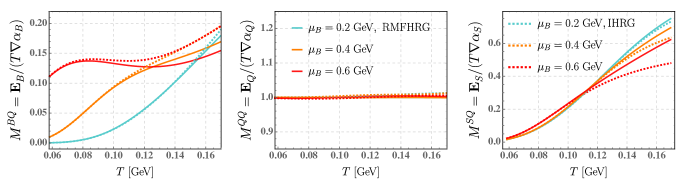
Until now, we have discussed the case that the gradients of conserved charge densities are completely directly converted to the diffusion currents. As mentioned in the introduction, the gradients of conserved charge densities can also produce an electric field, which in turn affects the diffusion currents of conserved charges. To exhibit the response of the electric field to conserved charge chemical thermal potential gradients, we display the variation of diffusion thermopower matrix with and in both the IHRG and RMFHRG models. As shown in Fig. 3, we observe that both and are increasing functions with , whereas the almost remains unchanged and approaches 1. This behavior of can well be understood from Eq. (43), where is almost in magnitude equal to . We note is the smallest, meaning the hadron gas (mainly protons) has a weak ability to convert the gradient of baryon chemical thermal potential into an electric field. With increasing , we see that visibly increases, while at high , for different gradually converge. The decrease of with in high region due to that the strong dependence of on dominates over the decreasing nature of with . In Fig. 3, we also observe that the RMF correction can give a significant enhancement on and reduction on at high , such responses mainly stem from and , respectively.

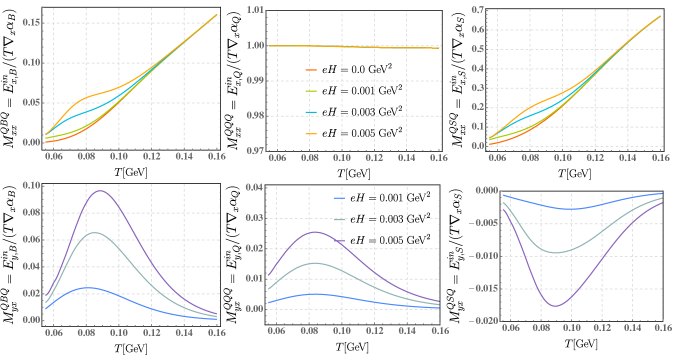
To intuitively exhibit the impact of the thermoelectric effect on the diffusion coefficient matrix, in Fig. 4 we give a comparison between and in the RMFHRG model. Once the thermoelectric effect is considered, diffusion coefficients in the electric charge sector vanish, only diffusion coefficients in the baryon and strangeness sectors exist. We first discuss the diffusion coefficients in the baryon sector. In the upper panel of Fig. 4 we see that the is nearly unaffected by the thermoelectric effect, which can be well understood from Eq. (45) that the product of and is so nominal in magnitude compared to . The thermoelectric effect can enhance , which further reduces the net baryon current. It’s worth noting that the thermoelectric effect can significantly suppress (), making () much smaller than () and even changing the sign. This means that the thermoelectric effect significantly decouples the correlation between electric current and baryon (strangeness) current, making the gradient of electric chemical potential insignificant for baryon (strangeness) diffusion. Hence, the baryon diffusion current can be reduced by the thermoelectric effect, and if gradients have comparable magnitude. As shown in the lower left panel of Fig. 4, the inclusion of thermoelectric effect does not explicitly break the symmetry between and . Different from , we observe that the inclusion of the thermoelectric effect can obviously decrease , as a result, the strangeness diffusion current has a significant reduction. We remark that the and dependence of is still consistent with that of .
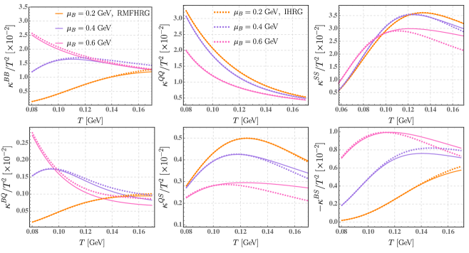
IV.2 Results for finite magnetic field
We also study the magneto-thermoelectric effect of hadronic matter and examine its impact on both the magnetic field-dependent diffusion coefficient matrix and the Hall-like diffusion coefficient matrix. So far, the realistic time evolution of initial magnetic field is unclear, according to the naive parametrization ( is the pion mass) for Au+Au collisions with fixed collision parameter Deng:2012pc , using with , for the thermalization timescale fm, we can get for the hadronization time scale fm. In this work, the magnetic field region is taken , as done in Ref. Das:2020beh .
All the estimations at finite magnetic fields are performed in the RMFHRG model with a fixed baryon chemical potential GeV. As shown in the upper panel of Fig. 5, the temperature dependence of scaled magnetic field-dependent thermoelectric conductivities at the finite magnetic field is unchanged compared with that at zero magnetic field. It is observed that at the finite magnetic field first increases with temperature and finally decreases. Such non-monotonic behavior of with mainly is the convoluted result between magnetic field effect and relaxation time in the integrand of Eq. (56), which can be well understood in analogy with the detailed discussion about magnetic field-dependent electric conductivity in Refs. Das:2019wjg ; Zhang:2020efz . The dominant carries of are charged pions, the scattering rate of pions at low is smaller than , leading , the pion scattering rate at high is much larger than , making . As a result, all the scaled magnetic field-dependent thermoelectric conductivities first decrease as the magnetic field increases and finally converge at high . From the lower panel of Fig. 5 we also note that all the scaled Hall-like thermoelectric conductivities exhibit a non-monotonic temperature dependence, which is due to the convolution between multiple factors, e.g. the relaxation time, the cyclotron frequency, as well as the factor . In the hadron gas, the predominant protons (p) and Sigma baryons () contribute to . We observe that is negative, this can be analyzed from Eq. (56), in which the dominant integrand term makes the sign of determined by the strangeness of Sigma baryons. The dependence of on the magnetic field is non-monotonic just because the proton scattering rate in low region is much smaller than the associated , leading , while in high region, the proton scattering rate plays a dominant role, , and then . For the , its dependence on the magnetic field almost is monotonic just because the scattering rate of predominant Sigma baryons is always larger than in the entire considered region. We also note the magnetic field dependence of is similar to that of , but its sign is different at low and high . This is because the behaviors of at low (high) are determined by the contribution from protons (Sigma baryons).
Next, we discuss the qualitative behaviors of both magnetic field-dependent diffusion thermopower matrix and Hall-like diffusion thermopower matrix with temperature and magnetic field, respectively. As shown in the upper panel of Fig. 6, the magnetic field effect gives an enhancement on both and in low region, which means the ability of hadron gas to convert baryon and strangeness chemical potential gradients to the electric field is strengthened by adding magnetic field, whereas the seems almost magnetic field-independent. All show a strong dependence on the magnetic field in the studied temperature region. As in the lower panel of Fig. 6, all in magnitude shows a similar peak structure in the entire region and increases as increases. We also note that is comparable in magnitude with the at low .
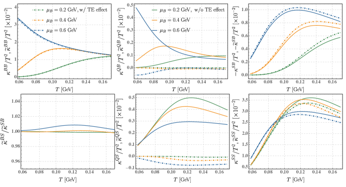
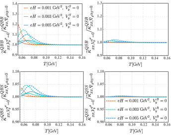
As in the case of the vanishing magnetic field, we also compare the magnetic field-dependent diffusion coefficient matrix before and after incorporating the magneto-thermoelectric effect in Fig. 7. We note that all except can not change their shape in the presence of magnetic field, the associated explanation of is similar to that of . As shown in Fig. 7, and in the baryon sector seem insensitive to magnetic field, while the remaining terms have significant reductions in the low region due to the inclusion of magnetic field. Thus, the presence of a magnetic field can significantly hinder the baryon and electric diffusion if gradients have similar magnitudes. The qualitative behavior of the magneto-thermoelectric modified diffusion coefficient matrix () is consistent with the non-modified one (). The symmetry between and still is satisfied as shown in the illustration of the upper right panel of Fig. 7.
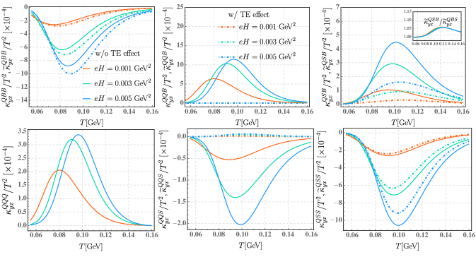
Compared with , all Hall-like diffusion coefficient matrix elements as in Fig. 8 exhibit a strong dependence on the magnetic field and show a peak structure in magnitude. The associated explanation of with and is similar to that of . We also note that have obvious responses to the magneto-thermoelectric effect. Similar to (), the magneto-thermoelectric effect can significantly suppress the magnitude of (), making the transverse coupling between electric charge and baryon (strangeness) charge nonsignificant in Hall-like baryon (strangeness) current. Strikingly different from , we find that the magneto-thermoelectric effect can give an obvious enhancement on the magnitude of . The and dependence of still similar to that of . One key finding is that the presence of magneto-thermoelectric effect causes a significant asymmetry between and , as shown in the illustration of the upper right panel of Fig. 8. With the increase of , the degree of asymmetry can be strengthened further.
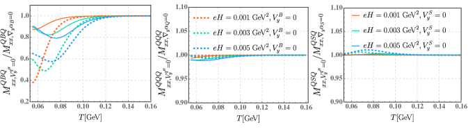
The above calculations in terms of magnetic field-dependent diffusion thermopower matrix and magneto-thermoelectric modified diffusion coefficient matrix in the magnetic field background are carried out under the assumption that the conserved charge chemical thermal potential gradients are only limited to the longitudinal direction, i.e., . As mentioned in Sec. III, under the condition of vanishing transverse diffusion current of conserved charge, i.e., with , a transverse gradient can be generated by , subsequently induces a transverse electric field. In such conditions, the magnitude of the magneto-thermoelectric modified diffusion coefficient matrix may be different from the counterpart under the condition of . In Fig. 9, we present the ratio of magnetic field-dependent diffusion thermopower under the conditions of and to the magnetic field-dependent diffusion thermopower in the condition of to intuitively quantify the difference due to the choice of transverse conditions. We find that choosing the condition of can lead to an obvious reduction on in low region, whereas both and show almost insensitive with varying transverse conditions. This result is unsurprising since, under the condition of , the () is much smaller than () as illustrated in Fig. 6, and the is always less than due to , as a result, the product of () and in Eq. (66) is nominal compared to ().
Finally, we show the sensitivity of magneto-thermoelectric modified diffusion coefficient matrix to the various choices of transverse conditions in Fig. 10. We don’t present the results for and because they are of a small order of magnitude compared to the other terms. We observe that taking the magneto-thermoelectric modified diffusion coefficient matrix in the condition of as a baseline, the variation of due to the change in transverse conditions is small, except that can have a significant reduction in the condition of at low .
V summary
We studied the thermoelectric effect and diffusion process of multiple conserved charges in hot and dense hadronic matter. Their corresponding diffusion thermopower matrix and diffusion coefficient matrix with were evaluated in both the IHRG and RMFHRG models by solving the relativistic Boltzmann equation in relaxation time approximation, where the Landau-Lifshitz energy frame was imposed. In the RMFHRG model, the repulsive interaction between hadrons was treated as a density-dependent mean-field potential, leading to a shift in the single-particle energy. In the magnetic field, the additional Hall-like diffusion thermopower matrix and Hall-like diffusion coefficient matrix can emerge. We further explored the impact of magneto-thermoelectric effect on and . The sensitivity of magnetic field-dependent diffusion thermopower matrix and magneto-thermoelectric modified diffusion coefficient matrix () to different transverse restrictions has also been studied. Here are our main results.
-
•
All diffusion coefficients except are sensitive to the RMF interaction in the baryon-rich region, which means the repulsive interaction between hadrons is vital in the diffusion properties of QCD matter created in the lower collision energies.
-
•
Both and exhibit a strong dependence on and , whereas, the almost remains unchanged with varying and , and nearly equal to 1. The RMF correction can significantly enhance (reduce) () at large .
-
•
The thermoelectric effect generally prevents the baryon (strangeness) diffusion, and in particular, significantly decouples the correlation between electric charge and baryon number (strangeness).
-
•
In the magnetic field, both and increase with the magnetic field at low , whereas the is almost magnetic field independent. The magnitude of the complete Hall-like diffusion thermopower matrix is strongly affected by and exhibits a peak structure in the considered region. Compared to and , the magnitude of at low is sensitive to the choices of various transverse restriction conditions.
-
•
Apart from and , remaining diffusion coefficients are sensitive to , and decrease with at low . This means that the magnetic field can prevent electric charge and strangeness diffusion. The quantitative and qualitative characteristics of magneto-thermoelectric modified diffusion coefficients remain relatively stable under varying transverse restriction conditions.
-
•
The full Hall-like diffusion coefficients in magnitude have a similar peak structure in the considered region and exhibit strong magnetic field dependence. It’s noted that the symmetry between the strangeness-baryon diffusion coefficient and baryon-strangeness diffusion coefficient could be broken after including the magneto-thermoelectric effect, i.e., .
These findings could offer valuable insights into the dynamics of distinct conserved charges and contribute to the development of dissipative (magneto-)hydrodynamics that explicitly account for multiple conserved charges.
Acknowledgements.
This work was supported by Guangdong Major Project of Basic and Applied Basic Research (2020B0301030008), the Natural Science Foundation of China (12247132), and the China Postdoctoral Science Foundation (2023M731159).appendix
In Fig. 11, we present a comparison between the diffusion coefficient matrix result in this investigation and the diffusion coefficient matrix result from A. Das et al Das:2021bkz within the IHRG model. In Ref. Das:2021bkz , the diffusion coefficient matrix is obtained as
| (75) | |||||
with being the equilibrium distribution function in the classical limit, i.e., the Boltzmann distribution function. As shown in Fig. 11, it’s clear that our full diffusion coefficient results are close to the results of A. Das et al. The small numerical discrepancy mainly comes from the different choices in degrees of freedom and the lack of quantum statistic effect in Das:2021bkz .
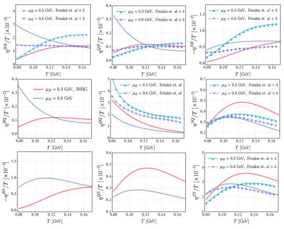
Alternatively, we note that the expression of , which has been derived in Refs Fotakis:2019nbq ; Greif:2017byw ; Fotakis:2021diq is different from ours. In Refs. Fotakis:2019nbq ; Greif:2017byw ; Fotakis:2021diq , it is given as
| (76) | |||||
| (77) |
In Ref. Fotakis:2019nbq , a constant relaxation time for all the hadron species is used. Comparing with the thermoelectric transport coefficient in Eq. (41), the is formally similar to the obtained in Refs. Fotakis:2019nbq ; Greif:2017byw ; Fotakis:2021diq by ignoring the quantum statistic effect and repulsive mean-field effect. As shown in Fig. 12, our results are smaller than the results in Ref. Fotakis:2019nbq , and the qualitative behaviors of in the baryon current are also slightly different to the results in Ref. Fotakis:2019nbq . It is clear that in Fig. 12 is not equivalent to at GeV. This means that the symmetry of the off-diagonal diffusion coefficients () illustrated in Refs. Fotakis:2019nbq ; Greif:2017byw is not strictly valid once the quantum statistic effect is considered. Comparing Fig. 2 and Fig. 12, we also observe that the quantitative and qualitative discrepancy between and is minimal, thus the numerical discrepancy between the diffusion coefficient matrix in this investigation and in Ref. Fotakis:2019nbq mainly stems from the numbers of degrees of freedom and relaxation time.
References
- (1) I. Arsene et al. [BRAHMS], Nucl. Phys. A 757, 1-27 (2005)
- (2) B. B. Back et al. [PHOBOS], Nucl. Phys. A 757, 28-101 (2005).
- (3) K. Adcox et al. [PHENIX], Nucl. Phys. A 757, 184-283 (2005).
- (4) J. Adams et al. [STAR], Nucl. Phys. A 757, 102-183 (2005).
- (5) K. Aamodt et al. [ALICE], Phys. Rev. Lett. 105, 252301 (2010).
- (6) S. Chatrchyan et al. [CMS], JHEP 08, 141 (2011).
- (7) G. Aad et al. [ATLAS], Phys. Lett. B 707, 330-348 (2012).
- (8) S. Chatrchyan et al. [CMS], Eur. Phys. J. C 72, 2012 (2012).
- (9) S. Chatrchyan et al. [CMS], Phys. Rev. C 84, 024906 (2011).
- (10) K. Aamodt et al. [ALICE], Phys. Lett. B 696, 30-39 (2011).
- (11) Y. Aoki, G. Endrodi, Z. Fodor, S. D. Katz and K. K. Szabo, Nature 443, 675-678 (2006).
- (12) M. Cheng, N. H. Christ, S. Datta, J. van der Heide, C. Jung, F. Karsch, O. Kaczmarek, E. Laermann, R. D. Mawhinney and C. Miao, et al. Phys. Rev. D 74, 054507 (2006).
- (13) O. Philipsen, Prog. Part. Nucl. Phys. 70, 55-107 (2013).
- (14) Y. Nambu and G. Jona-Lasinio, Phys. Rev. 122, 345-358 (1961).
- (15) T. Hatsuda and T. Kunihiro, Phys. Rept. 247, 221-367 (1994).
- (16) K. Fukushima, Phys. Rev. D 77, 114028 (2008) [erratum: Phys. Rev. D 78, 039902 (2008)].
- (17) B. J. Schaefer and J. Wambach, Phys. Rev. D 75, 085015 (2007).
- (18) B. J. Schaefer and M. Wagner, Phys. Rev. D 79, 014018 (2009).
- (19) B. J. Schaefer, J. M. Pawlowski and J. Wambach, Phys. Rev. D 76, 074023 (2007).
- (20) B. J. Schaefer and M. Wagner, Phys. Rev. D 85, 034027 (2012).
- (21) R. A. Lacey, Phys. Rev. Lett. 114, no.14, 142301 (2015).
- (22) M. M. Aggarwal et al. [STAR], [arXiv:1007.2613 [nucl-ex]].
- (23) B. Mohanty [STAR], J. Phys. G 38, 124023 (2011).
- (24) N. A. Tahir, C. Deutsch, V. E. Fortov, V. Gryaznov, D. H. H. Hoffmann, M. Kulish, I. V. Lomonosov, V. Mintsev, P. Ni and D. Nikolaev, et al. Phys. Rev. Lett. 95, 035001 (2005).
- (25) T. Ablyazimov et al. [CBM], Eur. Phys. J. A 53, no.3, 60 (2017).
- (26) B. Friman, C. Hohne, J. Knoll, S. Leupold, J. Randrup, R. Rapp, and P. Senger, The CBM Physics Book: Compressed Baryonic Matter in Laboratory Experiments (Springer, New York, 2011).
- (27) V. Kekelidze, R. Lednicky, V. Matveev, I. Meshkov, A. Sorin and G. Trubnikov, Phys. Part. Nucl. Lett. 9, 313-316 (2012).
- (28) P. Romatschke and U. Romatschke, Phys. Rev. Lett. 99, 172301 (2007).
- (29) P. Kovtun, D. T. Son and A. O. Starinets, Phys. Rev. Lett. 94, 111601 (2005).
- (30) U. Heinz and R. Snellings, Ann. Rev. Nucl. Part. Sci. 63, 123-151 (2013).
- (31) C. Sasaki and K. Redlich, Phys. Rev. C 79, 055207 (2009).
- (32) F. Karsch, D. Kharzeev and K. Tuchin, Phys. Lett. B 663, 217-221 (2008).
- (33) V. Roy, S. Pu, L. Rezzolla and D. Rischke, Phys. Lett. B 750, 45-52 (2015).
- (34) V. Roy, S. Pu, L. Rezzolla and D. H. Rischke, Phys. Rev. C 96, no.5, 054909 (2017).
- (35) M. Greif, J. A. Fotakis, G. S. Denicol and C. Greiner, Phys. Rev. Lett. 120, no.24, 242301 (2018).
- (36) J. A. Fotakis, M. Greif, C. Greiner, G. S. Denicol and H. Niemi, Phys. Rev. D 101, no.7, 076007 (2020).
- (37) J. A. Fotakis, O. Soloveva, C. Greiner, O. Kaczmarek and E. Bratkovskaya, Phys. Rev. D 104, no.3, 034014 (2021).
- (38) A. Das, H. Mishra and R. K. Mohapatra, Phys. Rev. D 106, no.1, 014013 (2022).
- (39) H. X. Zhang, J. W. Kang and B. W. Zhang, Eur. Phys. J. C 81, no.7, 623 (2021).
- (40) A. Das and H. Mishra, Eur. Phys. J. ST 230, no.3, 607-634 (2021).
- (41) H. X. Zhang, Y. X. Xiao, J. W. Kang and B. W. Zhang, Nucl. Sci. Tech. 33, no.11, 150 (2022).
- (42) M. Kurian, Phys. Rev. D 103, no.5, 054024 (2021).
- (43) D. Dey and B. K. Patra, Phys. Rev. D 102, no.9, 096011 (2020).
- (44) D. Dey and B. K. Patra, Phys. Rev. D 104, 076021 (2021).
- (45) S. A. Khan and B. K. Patra, Phys. Rev. D 107, no.7, 074034 (2023).
- (46) A. Das, H. Mishra and R. K. Mohapatra, Phys. Rev. D 102, no.1, 014030 (2020).
- (47) J. R. Bhatt, A. Das and H. Mishra, Phys. Rev. D 99, no.1, 014015 (2019).
- (48) S. Y. F. Liu and Y. Yin, Phys. Rev. D 104, no.5, 054043 (2021).
- (49) B. Fu, L. Pang, H. Song and Y. Yin, [arXiv:2201.12970 [hep-ph]].
- (50) V. Voronyuk, V. D. Toneev, W. Cassing, E. L. Bratkovskaya, V. P. Konchakovski and S. A. Voloshin, Phys. Rev. C 83, 054911 (2011).
- (51) K. Tuchin, Phys. Rev. C 83, 017901 (2011).
- (52) L. McLerran and V. Skokov, Nucl. Phys. A 929, 184-190 (2014).
- (53) J. Cleymans and K. Redlich, Phys. Rev. C 60, 054908 (1999).
- (54) F. Becattini, J. Cleymans, A. Keranen, E. Suhonen and K. Redlich, Phys. Rev. C 64, 024901 (2001).
- (55) D. H. Rischke, M. I. Gorenstein, H. Stoecker and W. Greiner, Z. Phys. C 51, 485-490 (1991).
- (56) A. Andronic, P. Braun-Munzinger, J. Stachel and M. Winn, Phys. Lett. B 718, 80-85 (2012).
- (57) G. P. Kadam and H. Mishra, Phys. Rev. C 92, no.3, 035203 (2015).
- (58) V. Vovchenko, M. I. Gorenstein and H. Stoecker, Phys. Rev. Lett. 118, no.18, 182301 (2017).
- (59) V. Vovchenko, A. Motornenko, P. Alba, M. I. Gorenstein, L. M. Satarov and H. Stoecker, Phys. Rev. C 96, no.4, 045202 (2017).
- (60) P. Huovinen and P. Petreczky, Phys. Lett. B 777, 125-130 (2018).
- (61) S. Pal, G. Kadam and A. Bhattacharyya, [arXiv:2305.13212 [hep-ph]].
- (62) G. Kadam and H. Mishra, Phys. Rev. D 100, no.7, 074015 (2019).
- (63) S. Pal, G. Kadam, H. Mishra and A. Bhattacharyya, Phys. Rev. D 103, no.5, 054015 (2021).
- (64) K. A. Olive, Nucl. Phys. B 190, 483-503 (1981).
- (65) J. Weil et al. [SMASH], Phys. Rev. C 94, no.5, 054905 (2016).
- (66) P. Chakraborty and J. I. Kapusta, Phys. Rev. C 83, 014906 (2011).
- (67) M. Albright and J. I. Kapusta, Phys. Rev. C 93, no.1, 014903 (2016).
- (68) J. L. Anderson and H. R. Witting, Physica 74, 466 (1974).
- (69) J. A. Fotakis, E. Molnár, H. Niemi, C. Greiner and D. H. Rischke, Phys. Rev. D 106, no.3, 036009 (2022).
- (70) E. Molnar, H. Niemi and D. H. Rischke, Phys. Rev. D 93, no.11, 114025 (2016).
- (71) R. Derradi de Souza, T. Koide and T. Kodama, Prog. Part. Nucl. Phys. 86, 35-85 (2016).
- (72) Callen, H. B. (1948). The Application of Onsager’s Reciprocal Relations to Thermoelectric, Thermomagnetic, and Galvanomagnetic Effects. Physical Review, 73(11), 1349–1358.
- (73) Redin, R. D., Thermomagnetic and galvanomagnetic effects (1957). Ames Laboratory ISC Technical Reports. 176.
- (74) M. E. Peskin and D. V. Schroeder, An Introduction to quantum field theory, Addison-Wesley, 1995, ISBN 978-0-201-50397-5.
- (75) C. Greiner, P. Koch and H. Stoecker, Phys. Rev. Lett. 58, 1825-1828 (1987).
- (76) J. Cleymans and H. Satz, Z. Phys. C 57, 135-148 (1993).
- (77) V. Vovchenko and H. Stoecker, Comput. Phys. Commun. 244, 295-310 (2019).
- (78) J. Cleymans, H. Oeschler, K. Redlich and S. Wheaton, Phys. Rev. C 73, 034905 (2006).
- (79) G. Odyniec, J. Phys. Conf. Ser. 455, 012037 (2013).
- (80) B. Aboona et al. [STAR], Phys. Rev. Lett. 130, no.8, 082301 (2023).
- (81) J. Hammelmann, J. Staudenmaier and H. Elfner, [arXiv:2307.15606 [nucl-th]].
- (82) J. Grefa, M. Hippert, J. Noronha, J. Noronha-Hostler, I. Portillo, C. Ratti and R. Rougemont, Phys. Rev. D 106, no.3, 034024 (2022)
- (83) R. Rougemont, J. Noronha and J. Noronha-Hostler, Phys. Rev. Lett. 115, no.20, 202301 (2015).
- (84) W. T. Deng and X. G. Huang, Phys. Rev. C 85, 044907 (2012).
- (85) A. Das, H. Mishra and R. K. Mohapatra, Phys. Rev. D 99, no.9, 094031 (2019), Phys. Rev. D 101, no.3, 034027 (2020).