Projected Gradient Descent Algorithm for Low-Rank Matrix Estimation

Abstract

Most existing methodologies of estimating low-rank matrices rely on Burer-Monteiro factorization, but these approaches can suffer from slow convergence, especially when dealing with solutions characterized by a large condition number, defined by the ratio of the largest to the $r$-th singular values, where $r$ is the search rank. While methods such as Scaled Gradient Descent have been proposed to address this issue, such methods are more complicated and sometimes have weaker theoretical guarantees, for example, in the rank-deficient setting. In contrast, this paper demonstrates the effectiveness of the projected gradient descent algorithm. Firstly, its local convergence rate is independent of the condition number. Secondly, under conditions where the objective function is rank-$2r$ restricted $L$-smooth and $\mu$-strongly convex, with $L/\mu<3$, projected gradient descent with appropriate step size converges linearly to the solution. Moreover, a perturbed version of this algorithm effectively navigates away from saddle points, converging to an approximate solution or a second-order local minimizer across a wide range of step sizes. Furthermore, we establish that there are no spurious local minimizers in estimating asymmetric low-rank matrices when the objective function satisfies $L/\mu<3.$

Keywords: low-rank matrix estimation, projected gradient descent, ill-conditioned matrix recovery, nonconvex optimization

1 Introduction

Low-rank matrix estimation plays a critical role in fields such as machine learning, signal processing, imaging science, and many others. This paper addresses the fundamental problem of low-rank matrix estimation:

$$\mathbf{X}_{*}=\operatorname*{arg\;min}_{\mathbf{X}\in\mathbb{R}^{n\times n}:\,\mathrm{rank}(\mathbf{X})=r}f(\mathbf{X}),$$ (1)

where the search rank $r$ is less than the matrix dimension $n$. In practical scenarios, the matrix size $n$ tends to be large. Consequently, contemporary approaches often adopt a nonconvex strategy pioneered by Burer and Monteiro (2003), which is to factorize an $n\times n$ candidate matrix $\mathbf{X}$ into its factor matrices and to directly optimize over the factors using a local optimization algorithm. Numerous studies have demonstrated the efficacy of this method and established its theoretical guarantees (Curtis et al., 2016; Zheng and Lafferty, 2016; Boumal et al., 2018; Zhang, 2022; Park et al., 2017; Boumal et al., 2016).

However, this method comes with certain limitations. Defining the “effective condition number” of $\mathbf{X}$ by

$$\kappa(\mathbf{X})=\frac{\sigma_{1}(\mathbf{X})}{\sigma_{r}(\mathbf{X})},$$

then one such limitation is evident when the effective condition number of $\mathbf{X}_{*}$ is large. While this method converges linearly, in order to achieve a certain accuracy, the number of iterations must increase linearly as the effective condition number $\kappa(\mathbf{X}_{*})$. This phenomenon is observed in numerous works (Zheng and Lafferty, 2015; Tu et al., 2016), summarized in (Tong et al., 2021, Table 1), and studied theoretically in (Bhojanapalli et al., 2016b, Theorem 3.3), which establishes a global convergence rate that depends on $1/\sigma_{r}(\mathbf{X}_{*})$. In the specific scenario where $\kappa(\mathbf{X}_{*})=\infty$, indicating a rank-deficient case with $\mathrm{rank}(\mathbf{X}_{*})<r$, Zhang et al. (2023) demonstrate that the gradient descent algorithm exhibits a slow and sublinear convergence rate.

To improve convergence rates in scenarios characterized by large $\kappa(\mathbf{X}_{*})$, Tong et al. (2021) introduced a novel approach: the scaled gradient descent (ScaledGD) algorithm. This method employs a preconditioned and diagonally-scaled gradient descent scheme, enabling linear convergence rates that are unaffected by $\kappa(\mathbf{X}_{*})$. However, Zhang et al. (2023) caution that it may not fare well in rank-deficient settings. To address this limitation, Zhang et al. (2023) proposed PrecGD, an extension of ScaledGD incorporating additional regularization within the preconditioner. Their research illustrates that within a localized vicinity surrounding the ground truth, PrecGD exhibits linear convergence towards the true solution, irrespective of $\kappa(\mathbf{X}_{*})$. Importantly, PrecGD also exhibits linear convergence in rank-deficient scenarios. However, it is worth noting that PrecGD demands careful selection of regularization parameters, both in theoretical considerations and practical implementation. Ma et al. (2023a) also addressed the issue by introducing a regularization parameter to ScaledGD, and showed that it converges at a constant linear rate independent of the condition number, but it requires a small initialization.

In this study, we focus on the projected gradient descent (ProjGD) algorithm, also known as the SVP algorithm in some previous literature (Jain et al., 2010; Zhang et al., 2021). Unlike ScaledGD or PrecGD, this algorithm stands out for its simplicity, devoid of the need for any regularization or preconditioner, and works well in practice.

1.1 Main Results

The primary contribution of this research lies in demonstrating the efficacy of the projected gradient descent algorithm, showcasing its robust performance irrespective of the condition number $\kappa(\mathbf{X}_{*})$.

Specifically, our key contributions can be outlined as follows:

• Firstly, we investigate the local convergence properties of ProjGD, revealing its ability to converge linearly at a rate independent of the condition number $\kappa(\mathbf{X}_{*})$. Our analysis yields a convergence rate that improves over existing works.

• Secondly, we explore the global convergence behavior of ProjGD. We establish that under conditions where the function is $2r$-restricted $L$-smooth and $\mu$-strongly convex, and $L/\mu<3$, when applied with an appropriate step size, ProjGD converges linearly to the solution, with a rate remains unaffected by $\kappa(\mathbf{X}_{*})$. Compared to existing works, our result expands the allowable range for $L/\mu$ and step size.

• Finally, we introduce a perturbed variant of ProjGD, demonstrating its ability to converge to an approximate critical point of $f$ in $\mathbb{R}^{n\times n}$ or a second-order local minimizer of $f$ on the manifold of low-rank matrices, under relaxed assumptions regarding step sizes. Our definition of second-order local minimizers applies directly to the low-rank matrices themselves, rather than their factorizations (Zhang et al., 2023). This distinction strengthens our result.

• Additionally, this paper establishes the absence of spurious local minimizers when $L/\mu<3$, which extends the findings of (Zhang, 2022, Corollary 1.2) to the asymmetric matrix setting, employing a distinct proof strategy.

1.2 Related literature

While the low-rank matrix estimation problem has garnered significant attention in the literature, the related literature to this work can be categorized into five distinct areas: landscape of low-rank matrix estimation, projected gradient algorithms, ill-conditioned estimation, rank-deficient setting, and saddle point avoidance.

No spurious local minimizer in low-rank matrix estimation The matrix sensing problem has been extensively investigated in the literature, particularly regarding the absence of spurious local minima under certain conditions under a restricted isometry property (RIP) condition (Ge et al., 2017; Bhojanapalli et al., 2016b; Zhang et al., 2019). Notably, Bhojanapalli et al. (2016b) focused on the positive definite setting, demonstrating the convergence of noisy gradient descent to a global optimum under conditions such as $(2r,\frac{1}{10})$-RIP for the noisy case and $(2r,\frac{1}{5})$-RIP for the clean case. Similarly, Park et al. (2017) addressed the asymmetric matrix sensing problem under $(4r,0.0363)$-RIP for the clean case and $(4r,0.02)$-RIP for the noisy case. Ge et al. (2017) provided insights into the noiseless case, demonstrating that under the $(2r,\frac{1}{10})$-RIP condition, spurious local minima are absent in the positive semidefinite (PSD) setting; and under $(2r,\frac{1}{20})$-RIP, the absence of local minima is ensured in the asymmetric setting. Zhang et al. (2018, 2019, 2021) contributed further by showing that $(2r,1/2)$-RIP guarantees the absence of spurious solutions, and demonstrated through a counterexample that the non-existence of spurious second-order critical points may not hold if it does not hold. Molybog et al. (2021) investigated sparse operators with low-dimensional representations, establishing necessary and sufficient conditions for the absence of spurious solutions under coherence and assumed structure. They highlighted that combining sparsity and structure can render the coherence assumption almost redundant. Several other works have also made significant contributions to the study of this phenomenon (Ha et al., 2020; Bi and Lavaei, 2021).

Researchers have also investigated the absence of spurious local minima for generic matrix functions beyond the matrix sensing problem. Zhu et al. (2018) examined the estimation of asymmetric setting and established that spurious local minima are nonexistent when the condition number of the objective function $\kappa_{f}=L/\mu$ is less than or equal to $1.5$. In a related vein, Zhang (2022) explored the symmetric setting and demonstrated that the presence of spurious local minima depends on the relationship between the search rank $r$ and the true rank $r_{*}$, along with the condition number of the objective function $\kappa_{f}$. Specifically, Zhang proved that spurious local minimizers are absent if $r$ exceeds the true rank $r_{*}$ by a factor of $\frac{1}{4}(\kappa_{f}-1)^{2}r_{*}$, while counterexamples exist if $r<\frac{1}{4}(\kappa_{f}-1)^{2}r_{*}-1$. Notably, without rank overparameterization, the absence of spurious minimizers holds if and only if $\kappa_{f}<3$.

Projected gradient descent (ProjGD) in low-rank matrix estimation Several studies have investigated the application of projected gradient descent in low-rank matrix estimation. For instance, Cai et al. (2018) utilized this technique for spectral compressed sensing, while Chen and Wainwright (2015) applied it to various tasks such as matrix regression, rank-r PCA with row sparsity, and low-rank and sparse matrix decomposition. However, both works require the step size to decrease to zero as the condition number $\kappa(\mathbf{X}_{*})$ increases to infinity, rendering them inapplicable to rank-deficient cases where $r_{*}<r$.

In contrast, several other studies investigated the projected gradient descent in low-rank matrix estimation, demonstrating its convergence to minimizers under certain assumptions and with specific choices of step sizes (Jain et al., 2010; Zhang et al., 2021; Ha et al., 2020). Notably, these analyses highlight that the convergence rate remains independent of $\kappa(\mathbf{X}_{*})$.

Factored gradient descent (FGD) in ill-conditioned low-rank matrix estimation Zhuo et al. (2021) provided a thorough analysis of over-parameterized low-rank matrix sensing using the FGD method. They highlighted that when $r>r_{*}$, existing statistical analyses fall short due to the flat local curvature of the loss function around the global maxima. In such cases, convergence initially follows a linear path to a certain error before transitioning to a sub-linear trajectory towards the statistical error.

Similarly, Tong et al. (2021) demonstrated that even when $r=r_{*}$, the convergence rate of FGD is linearly dependent on the condition number $\kappa(\mathbf{X}_{*})$. To address this, they proposed a preconditioned gradient descent approach called ScaledGD, which converges linearly at a rate independent of the condition number of the low-rank matrix, akin to alternating minimization. ScaledGD employs a preconditioner of the form $(\mathbf{X}^{T}\mathbf{X})^{-1}$. In a related vein, Zhang et al. (2023) proposed PrecGD by regularizing the preconditioner as $(\mathbf{X}^{T}\mathbf{X}+\eta\mathbf{I})^{-1}$ and demonstrated its linear convergence rate in the overparameterized case when initialized within a neighborhood around the ground truth, even in cases of degenerate or ill-conditioned settings. A perturbed version of PrecGD also achieves global convergence from any initial point. Additionally, a stochastic version is proposed in (Zhang et al., 2022).

Moreover, there is ongoing research exploring the relationship between factorization methods and rank-constrained techniques. Ha et al. (2020) demonstrated that all second-order stationary points of the factorized objective function correspond to fixed points of projected gradient descent applied to the original problem, where the projection step enforces the rank constraint. This finding enables the unification of optimization guarantees established in either the rank-constrained or factorized setting. Similarly, Luo et al. (2022) explored the equivalence between these two methods.

Rank-deficient low-rank matrix estimation In practical scenarios, the rank of the ground truth $r$ is often unknown. To address this uncertainty, it is common practice to conservatively select the search rank $r$ such that $r>r_{*}:=\mathrm{rank}(\mathbf{X}_{*})$. This approach entails overparameterizing the model, allocating more degrees of freedom than exist in the ground truth. For instance, in safety-critical applications where ensuring proof of quality is paramount, rank overparameterization ($r>r_{*}$) is coupled with trust region methods (Rosen et al., 2019, 2020; Boumal et al., 2018), albeit at a higher computational cost.

Such overparameterization/rank-deficient regime has been shown to perform well theoretically. Li et al. (2018) investigated gradient descent in the rank-deficient regime of noisy matrix sensing. They demonstrated that with a sufficiently good initialization, early termination of gradient descent yields a satisfactory solution, owing to implicit regularization effects. Stöger and Soltanolkotabi (2021) provided insights into rank-deficient low-rank matrix sensing, revealing that the trajectory of gradient descent iterations from small random initialization can be roughly decomposed into three distinct phases–spectral/alignment, saddle avoidance/refinement, and local refinement. Similarly, Ma and Fattahi (2023) investigated robust matrix recovery and demonstrate that overestimation of the rank has no impact on the performance of the subgradient method, provided that the initial point is sufficiently close to the origin. In addition, Zhang (2021) studied the landscape of general rank-deficient regime with $r_{*}\leq r$, establishing that $(\delta,r+r_{*})$-RIP with $\delta<1/(1+\sqrt{\frac{r_{*}}{r}})$ is sufficient for the absence of spurious local minima.

However, Zhuo et al. (2021) highlighted a limitation of the rank-deficient regime by demonstrating that while factored gradient descent converges unconditionally to a good solution, it does so at a sublinear rate.

It is worth noting an alternative method of overparameterization, as proposed in (Ma et al., 2023b), which relies on the lifting technique and the Burer-Monteiro factorization, distinct from the approach of setting $r>r_{*}$.

Escaping saddle points Given the nonconvex nature of the low-rank estimation problem, there is a compelling demand to explore saddle point-avoiding algorithms. Existing analyses of such algorithms often hinge on the so-called “strict saddle property”, ensuring that all local minimizers are close to the global minimizers, and for any saddle point of the objective function, its Hessian features a significant negative eigenvalue (Jin et al., 2017; Daneshmand et al., 2018; Zhang et al., 2023). Indeed, as demonstrated in (Ge et al., 2017, Theorem 3), the low-rank matrix sensing problem enjoys the strict saddle property when the RIP condition is met.

Lee et al. (2016) showcased that for generic problems, gradient descent almost surely converges to a local minimizer with random initialization. Furthermore, gradient descent algorithms can be tailored to steer clear of saddle points and converge solely to minimizers. Perturbed gradient descent, for instance, is deployed to evade saddle points with high probability (Jin et al., 2017, 2021), with extensions to linear constrained optimization (Lu et al., 2020), nonsmooth optimization (Davis et al., 2022; Davis and Drusvyatskiy, 2022; Huang, 2021), bilevel optimization (Huang et al., 2023), and manifold optimization (Sun et al., 2019; Vlatakis-Gkaragkounis et al., 2019). Additionally, stochastic gradient descent (SGD) is renowned for its capability to circumvent saddle or spurious local minima (Daneshmand et al., 2018). Beyond perturbations, a class of saddle-point avoiding algorithms utilizes second-order information (Nesterov and Polyak, 2006; Curtis et al., 2016; Agarwal et al., 2017; Carmon et al., 2018) to steer away from saddle points and toward minimizers.

1.3 Organization

The paper is structured as follows: Section 2 provides an overview of the problem setting and introduces the projected gradient descent algorithm. In Section 3, we present the main results of the paper, with key findings outlined in each subsection. Section 4 offers insights from numerical experiments. For technical proofs and supplementary experiments, refer to Section 6.

2 Background

2.1 Notation

For any $\mathbf{X}\in\mathbb{R}^{n_{1}\times n_{2}}$ with $\mathrm{rank}(\mathbf{X})=r_{0}$, we denote its singular values decomposition with $\mathbf{X}=\boldsymbol{U}_{\mathbf{X}}\boldsymbol{\Sigma}_{\mathbf{X}}\mathbf{V}^{T}_{\mathbf{X}}$, where $\boldsymbol{U}_{\mathbf{X}}\in\mathbb{R}^{n_{1}\times r_{0}},\boldsymbol{\Sigma}_{\mathbf{X}}\in\mathbb{R}^{r_{0}\times r_{0}},$ and $\mathbf{V}_{\mathbf{X}}\in\mathbb{R}^{n_{2}\times r_{0}}$. In particular, the singular values are $\sigma_{1}(\mathbf{X})\geq\sigma_{2}(\mathbf{X})\geq\cdots\geq\sigma_{r_{0}}(\mathbf{X})$ with the corresponding left and right singular vectors $\{\boldsymbol{u}_{i}(\mathbf{X})\}_{i=1}^{r_{0}}$ and $\{\boldsymbol{v}_{i}(\mathbf{X})\}_{i=1}^{r_{0}}$.

If $\mathrm{rank}(\mathbf{X})>r$, its rank-$r$ approximation is given by $\mathcal{P}_{r}(\mathbf{X})=\boldsymbol{U}_{\mathbf{X},r}\boldsymbol{\Sigma}_{\mathbf{X},r}\mathbf{V}^{T}_{\mathbf{X},r}$, where $\boldsymbol{U}_{\mathbf{X},r}\in\mathbb{R}^{n_{1}\times r}=[\boldsymbol{u}_{1}(\mathbf{X}),\cdots,\boldsymbol{u}_{r}(\mathbf{X})],\boldsymbol{\Sigma}_{\mathbf{X},r}\in\mathbb{R}^{r\times r}=\mbox{diag}(\sigma_{1}(\mathbf{X}),\cdots,\sigma_{r}(\mathbf{X})),$ and $\mathbf{V}_{\mathbf{X},r}\in\mathbb{R}^{n_{2}\times r}=[\boldsymbol{v}_{1}(\mathbf{X}),\cdots,\boldsymbol{v}_{r}(\mathbf{X})]$.

For any orthogonal matrices $\boldsymbol{U}\in\mathbb{R}^{n\times r}$, we use $\boldsymbol{U}^{\perp}$ to represent an orthogonal matrix in $\mathbb{R}^{n\times n-r}$ such that $[\boldsymbol{U},\boldsymbol{U}^{\perp}]^{T}[\boldsymbol{U},\boldsymbol{U}^{\perp}]=\mathbf{I}$, that is, the columns of $\boldsymbol{U}$ and $\boldsymbol{U}^{\perp}$ is an orthonormal basis of $\mathbb{R}^{n}$. In addition, we let $[\mathbf{X}]_{\boldsymbol{U},\mathbf{V}}=\boldsymbol{U}\boldsymbol{U}^{T}\mathbf{X}\mathbf{V}\mathbf{V}^{T}$ be the projection of the columns of $\mathbf{X}$ to $\mathrm{Sp}(\boldsymbol{U})$ and the projection of the rows of $\mathbf{X}$ to $\mathrm{Sp}(\mathbf{V})$.

In addition, for any matrix $\mathbf{X}$ with rank $r$, we use $T(\mathbf{X})$ to represent its tangent space at the manifold of all matrices of rank $r$:

$$T(\mathbf{X})=\{\mathbf{Z}_{1}\mathbf{X}+\mathbf{X}\mathbf{Z}_{2}:\mathbf{Z}_{1}\in\mathbb{R}^{n\times n},\mathbf{Z}_{2}\in\mathbb{R}^{n\times n}\}.$$

$P_{T(\mathbf{X})}:\mathbb{R}^{n\times n}\rightarrow\mathbb{R}^{n\times n}$ represents the projector to the subspace $T(\mathbf{X})$, and we have the following expression:

$$P_{\boldsymbol{T}(\mathbf{X})}(\mathbf{Z})=[\mathbf{Z}]_{\boldsymbol{U}_{\mathbf{X}},\mathbf{V}_{\mathbf{X}}}+[\mathbf{Z}]_{\boldsymbol{U}_{\mathbf{X}}^{\perp},\mathbf{V}_{\mathbf{X}}}+[\mathbf{Z}]_{\boldsymbol{U}_{\mathbf{X}},\mathbf{V}_{\mathbf{X}}^{\perp}}=\mathbf{Z}-[\mathbf{Z}]_{\boldsymbol{U}_{\mathbf{X}}^{\perp},\mathbf{V}_{\mathbf{X}}^{\perp}}.$$

We let ${\boldsymbol{T}(\mathbf{X})^{\perp}}$ be the subspace perpendicular to $\boldsymbol{T}(\mathbf{X})$ and the projector to ${\boldsymbol{T}(\mathbf{X})^{\perp}}$ can be written by

$$P_{\boldsymbol{T}(\mathbf{X})^{\perp}}\mathbf{Z}=[\mathbf{Z}]_{\boldsymbol{U}_{\mathbf{X}}^{\perp},\mathbf{V}_{\mathbf{X}}^{\perp}}.$$

2.2 Projected and factored gradient descent algorithms

Projected gradient descent (ProjGD) algorithm The projected gradient descent algorithm (ProjGD) treats (1) as a constrained optimization problem. It iteratively performs a gradient step and then projects the result to satisfy the constraints:

$$\mathbf{X}^{(t+1)}=\mathcal{P}_{r}\big{(}\mathbf{X}^{(t)}-\eta\nabla f(\mathbf{X}^{(t)})\big{)},$$ (2)

where $\mathcal{P}_{r}$ represents the projection to the nearest rank-$r$ matrix, computable using singular value decomposition.

It is worth noting that the projected gradient descent algorithm can be extended to the scenario where $\mathbf{X}$ is assumed to be symmetric and positive semidefinite (PSD) (Ge et al., 2017)., by employing

$$\mathcal{P}_{r}(\mathbf{X})=\sum_{i=1}^{r}\max(\lambda_{i}(\mathbf{X}),0)\boldsymbol{u}_{i}(\mathbf{X})\boldsymbol{u}_{i}(\mathbf{X})^{T}.$$

In this paper, we focus on the asymmetric setting for theoretical analysis while investigating both settings in simulations.
Factored gradient descent (FGD) algorithm Many state-of-the-art algorithms adopt a nonconvex approach pioneered by Burer and Monteiro (2003). This method involves factorizing an $n\times n$ candidate matrix $\mathbf{X}$ into its factor matrices $\mathbf{X}=\mathbf{L}\boldsymbol{R}^{T}$, where $\mathbf{L},\boldsymbol{R}\in\mathbb{R}^{n\times r}$, and directly optimizing over these factors using local optimization algorithms (Curtis et al., 2016; Zheng and Lafferty, 2016; Boumal et al., 2018; Zhang, 2022; Park et al., 2017; Boumal et al., 2016). Specifically, the standard Factored gradient descent (FGD) algorithm operates as follows:

$$\boldsymbol{U}^{(t+1)}= \big{(}\mathbf{X}^{(t)}-\eta\nabla f(\mathbf{X}^{(t)})\big{)}\mathbf{V}^{(t)},\,\,\mathbf{V}^{(t+1)}=\big{(}\mathbf{X}^{(t)}-\eta\nabla f(\mathbf{X}^{(t)})\big{)}\boldsymbol{U}^{(t)},\,\,\mathbf{X}^{(t+1)}=\boldsymbol{U}^{(t+1)}\mathbf{V}^{(t+1)\,T}.$$ (3)

Computational cost per iteration of projected and factored gradient descent While both algorithms require the computation of $\nabla f(\mathbf{X})$, ProjGD involves an additional step of rank-$r$ projection $\mathcal{P}_{r}$, whereas FGD incurs additional computational cost due to the multiplication steps over its factors. Despite these differences, both algorithms have a computational cost of $O(n^{2}r)$. Specifically, the multiplication between two $n\times r$ matrices in (3), as well as the multiplication between a matrix of size $n\times n$ and a matrix of size $n\times r$ in (3), also have a computational cost of $O(n^{2}r)$. Consequently, both algorithms have the same order of computational costs per iteration.

3 Main Results

In this section, we outline our main results. The first key finding, presented in Theorem 1, demonstrates that ProjGD converges locally at a rate independent of $\kappa(\mathbf{X}_{*})$. The second significant result, detailed in Theorem 2, establishes that if the function is rank-$2r$ restricted $L$-smooth and $\mu$-strongly convex, with $L/\mu<3$, then the projected gradient descent algorithm converges linearly to the solution with an appropriate choice of step size. Lastly, Theorem 3 illustrates that PprojGD, a perturbed version of ProjGD, converges to an approximate second-order local minimizer in the matrix of low-rank matrices, or an approximate stationary point in $\mathbb{R}^{n\times n}$. This implies that PprojGD converges to an approximate solution if $L/\mu<3$, with a broader range of step sizes to choose from. In addition, Corollary 1 proves that there is no spurious local minimizer when estimating asymmetric low-rank matrices under the condition $L/\mu<3$.

3.1 Local convergence of ProjGD

This section establishes the local convergence property of ProjGD (2), subject to Assumptions A1-A2 on $f$. These assumptions are standard and have been widely employed in works such as (Tong et al., 2021) and (Zhang et al., 2023). As discussed in (Tong et al., 2021, Section 2.5), numerous optimization problems satisfy Assumptions A1-A2, including low-rank matrix factorization, matrix completion, and low-rank matrix sensing.

Assumption A1 [Rank-$2r$ restricted smoothness and strong convexity]: The function $f$ satisfies the following conditions:

$$\|\nabla f(\mathbf{X})-\nabla f(\mathbf{X}^{\prime})\|_{F}\leq L\|\mathbf{X}-\mathbf{X}^{\prime}\|_{F}$$ (4)

and

$$\langle\nabla^{2}f(\mathbf{X})[\boldsymbol{E}],\boldsymbol{E}\rangle\geq\mu\|\boldsymbol{E}\|_{F}^{2}$$ (5)

for any $\mathbf{X},\mathbf{X}^{\prime},\boldsymbol{E}\in\mathbb{R}^{n\times n}$ with ranks no more than $r$.

Assumption A2 [Unconstrained minimizer is low-rank] The minimizer of function $f$

$$\mathbf{X}_{*}=\arg\min_{\mathbf{X}\in\mathbb{R}^{n\times n}}f(\mathbf{X})$$ (6)

satisfies that $\mathrm{rank}(\mathbf{X}_{*})=r_{*}\leq r$.

Our result, Theorem 1, demonstrates that the ProjGD algorithm converges linearly when well-initialized, with the convergence rate depending on the step size $\eta$, $L$, and $\mu$, but being independent of the effective condition number of the solution $\kappa(\mathbf{X}_{*})$.

Theorem 1.

[Local convergence rate] Under Assumptions A1-A2, there exists $c_{0}>0$ such that for any initialization $\mathbf{X}^{(0)}$ satisfying $f(\mathbf{X}^{(0)})-f(\mathbf{X}_{*})\leq 0.01\sigma_{r_{*}}(\mathbf{X}_{*})^{2}\mu/\kappa_{f}$, where $\kappa_{f}=L/\mu$, then ProjGD with a step size $\eta<1/2L$ converges linearly to $\mathbf{X}_{*}$, and the iterates of ProjGD satisfy the following condition:

$$\frac{f(\mathbf{X}^{(k+1)})-f(\mathbf{X}_{*})}{f(\mathbf{X}^{(k)})-f(\mathbf{X}_{*})}\leq 1-\frac{4}{27\kappa_{f}}\big{(}{\eta L}-\eta^{2}L^{2}\big{)}.$$

Comparison with existing results Theorem 1 highlights that the convergence rate relies on $\kappa_{f}$ and $\eta L$ and remains unaffected by the effective condition number $\kappa(\mathbf{X}_{*})$. In contrast, for FGD, the number of iterations required to achieve a certain accuracy increases linearly with the effective condition number (Tong et al., 2021). Moreover, when $r_{*}<r$, FGD experiences a slowdown to a sublinear local convergence rate, both theoretically and empirically (Zhang et al., 2023, Section 5). While ScaledGD by Zhang et al. (2023) and PrecGD by Zhang et al. (2023) also exhibit rates independent of the effective condition number $\kappa(\mathbf{X}_{*})$, the analysis of ScaledGD cannot handle the scenario $r_{*}<r$, and PrecGD requires a carefully chosen regularization parameter that varies with each iteration.

In particular, when we set $\eta=1/3L$ and let $\kappa_{f}=L/\mu$ being the condition number of the objective function $f$, ProjGD requires $O(\log(1/\epsilon)\cdot\kappa_{f})$ iterations to achieve an $\epsilon$-accuracy of $\|\mathbf{X}^{(k)}-\mathbf{X}_{*}\|<\epsilon$. In contrast, FGD has an iteration complexity of $O(\log(1/\epsilon)\cdot\kappa_{f}\cdot\kappa(\mathbf{X}_{*}))$ (Park et al., 2017; Bhojanapalli et al., 2016a), which is worse by a factor of $\kappa(\mathbf{X}_{*})$. Additionally, according to (Zhang et al., 2023, Theorem 4), PrecGD requires at least $O(\log(1/\epsilon)\cdot\kappa_{f}^{2})$ iterations, which is worse by a factor of $\kappa_{f}$. The only existing work with the same convergence rate is Theorem 4 in (Tong et al., 2021), demonstrating that ScaledGD shares the same iteration complexity of $O(\log(1/\epsilon)\cdot\kappa_{f})$. However, this theorem is only valid when $r_{*}=r$ and does not apply when $r_{*}<r$.

3.2 Global convergence of ProjGD

This section establishes that when $L/\mu<3$, ProjGD converges to the unique minimizer $\mathbf{X}_{*}$ with an appropriately chosen step size $\eta$. Compared to existing works, our result expands the permissible range of $L/\mu$ and offers greater flexibility in selecting the step size $\eta$.

Theorem 2.

(a) [Global convergence] Under Assumptions A1-A2, and assume in addition that $L/\mu<3$, then the ProjGD algorithm converges linearly to $\mathbf{X}_{*}$ for step sizes in the range

$$\frac{(L^{2}-\mu^{2})}{2L\mu(L+\mu)}<\eta<\frac{1}{L}.$$

(b) [Global convergence rate] Under the setting in (a), and let $\kappa_{0}=\frac{L-\mu}{L+\mu}$ and $\epsilon>0$ be chosen such that $\hat{\kappa}_{0}=\sqrt{\kappa_{0}^{2}+2\epsilon-2\epsilon^{2}}<1/2$, if we choose step size $\eta$ such that for $\eta_{0}=2\eta/(L+\mu)$, $1/(1/\hat{\kappa}_{0}-\hat{\kappa}_{0})<\eta_{0}<1/(1+\kappa_{0})$, then the iterates of ProjGD satisfy the following condition:

$$\frac{f(\mathbf{X}^{(k+1)})-f(\mathbf{X}_{*})}{f(\mathbf{X}^{(k)})-f(\mathbf{X}_{*})}\leq 1-\Big{(}\frac{1}{(1+\kappa_{0})\eta_{0}}-1\Big{)}\min\Bigg{(}\frac{\eta_{0}}{10},\frac{2\epsilon\eta_{0}}{3},\frac{1}{2\sqrt{r}}\Big{(}\eta_{0}-\frac{\hat{\kappa}_{0}}{{1-\hat{\kappa}_{0}^{2}}}\Big{)}\Bigg{)}^{2}.$$

We note that part (b) implies part (a): Since $\epsilon$ in part (b) can be chosen to be arbitrarily small so that $\hat{\kappa}_{0}$ is close to $\kappa_{0}$ and smaller than $\eta_{0}$, Theorem 2(b) implies Theorem 2(a).

Comparison with existing results Theorem 2 can be contrasted with existing works such as (Jain et al., 2010; Zhang et al., 2021; Ha et al., 2020). In particular, Zhang et al. (2021) extend the results by Jain et al. (2010) from matrix sensing to general matrix estimation problems and demonstrate that under the assumption of symmetry and $L/\mu\leq 2$, the ProjGD algorithm converges linearly to the minimizer with a rate of $O((\frac{2\kappa_{0}}{1-\kappa_{0}})^{k})$ when the step size is $\eta=1/L$. By adapting the proof of (Zhang et al., 2021, Theorem 3), it can be shown that linear convergence holds for step sizes $1/2\mu\leq\eta\leq 1/L$. It is worth noting that our theorem, Theorem 2, allows a larger range of $L/\mu<3$ and a larger range of step sizes, because $\frac{(L^{2}-\mu^{2})}{2L\mu(L+\mu)}\leq\frac{1}{2\mu}$. Similarly, Ha et al. (2020) demonstrated that when $L/\mu\leq 2$ and $1/2\mu\leq\eta\leq 1/L$, $\mathbf{X}_{*}$ is the unique stationary point of ProjGD.

To summarize, Theorem 2 improves upon existing results in two key aspects: Firstly, it applies to $L/\mu<3$ instead of the previous limit of $L/\mu\leq 2$. Secondly, its analysis allows for a wider range of step sizes, with a smaller lower bound. There are also some technical differences: compared to (Zhang et al., 2021), Theorem 2 addresses the asymmetric setting of $\mathbf{X}$ rather than being restricted to PSD matrices. Compared to (Ha et al., 2020), Theorem 2 offers additional insights into the rate of convergence.

3.3 Global convergence of perturbed projected gradient descent (PprojGD)

The requirement in Theorem 2 for an appropriately chosen step size may not be practical where the exact values of $L$ and $\mu$ are unknown. In practice, it is more typical to use a small fixed step size in gradient descent algorithms. However, there could be saddle points that serve as fixed points of ProjGD with small step sizes, as demonstrated in (Zhang et al., 2019, Section 6). This highlights a potential limitation of the theoretical results.

To explain this gap between theory and practice, we propose PprojGD (perturbed ProjGD) in Algorithm 1, drawing inspiration from Jin et al. (2017) and Criscitiello and Boumal (2019). PprojGD is designed to escape saddle points encountered by ProjGD. The key idea behind PprojGD is as follows: if ProjGD fails to induce a significant change in the estimate, indicated by a small Frobenius norm of the difference $\|\mathbf{X}^{(k+1)}-\mathbf{X}^{(k)}\|_{F}$, then the current iteration $\mathbf{X}^{(k)}$ is considered as an approximate saddle point. In such cases, PprojGD performs a tangent space step instead, which involves multiple perturbed gradient descent steps on the tangent space. The term “tangent space steps” is derived from (Criscitiello and Boumal, 2019) and is summarized in Algorithm 2.

It is worth noting a distinction between Algorithm 1 and the approach in Criscitiello and Boumal (2019). While the intuition behind both algorithms is similar, there is a difference in the criterion used to determine when to add perturbations. In Algorithm 1, rather than assessing the magnitude of gradient derivatives, we evaluate the Frobenius norm of the difference between consecutive iterates, $\|\mathbf{X}^{(k+1)}-\mathbf{X}^{(k)}\|_{F}$.

To formally describe Algorithm 2, let’s introduce the concept of a pullback of $f$ from $\mathcal{M}_{r}$, the manifold of matrices of size $n\times n$ and rank $r$, to its tangent space $T(\mathbf{X})$ at $\mathbf{X}\in\mathcal{M}_{r}$. We first define $\mathbf{Retr}:T(\mathbf{X})\rightarrow\mathbb{R}^{n\times n}$ as the inverse of projection $P_{T(\mathbf{X})}:\mathcal{M}_{r}\rightarrow T(\mathbf{X})$. Then we define the pullback of $f$ from $\mathcal{M}_{r}\rightarrow\mathbb{R}$ to $T(\mathbf{X})\rightarrow\mathbb{R}$ by $\hat{f}_{\mathbf{X}}=f\cdot\mathbf{Retr}_{\mathbf{X}}$. We refer the reader to (49) for a rigorous definition.

Algorithm 1 PprojGD: perturbed projected gradient descent

Input: Objective function $f:\mathbb{R}^{n\times n}\rightarrow\mathbb{R}$; initialization $\mathbf{X}^{(0)}\in\mathbb{R}^{n\times n}$; step size $\eta$; criterion for improvement $\epsilon$; eigenvalue threshold for tangent space steps $\epsilon_{T}$; parameters of tangent space steps $(r,\eta_{T},\mathcal{J})$; maximum number of iterations $\mathcal{T}$.

Output: Estimated $\mathbf{X}^{(\mathrm{iter})}$.

Steps:
1: Initialize $\mathrm{iter}=0$.

2: Compute $\mathbf{X}_{+}=\mathcal{P}_{r}\big{(}\mathbf{X}-\eta\nabla f(\mathbf{X})\big{)}$.

3: Set

$$\mathbf{X}^{(\mathrm{iter}+1)}=\begin{cases}\mathbf{X}_{+},&\text{if $\|\mathbf{X}_{+}-\mathbf{X}^{(\mathrm{iter})}\|_{F}\geq 2\eta\epsilon/3$}\\ \mathrm{TangentSpaceSteps}(\mathbf{X},r,\eta_{T},\epsilon_{T},\mathcal{J}),\,\,&\text{if $\|\mathbf{X}_{+}-\mathbf{X}^{(\mathrm{iter})}\|_{F}<2\eta\epsilon/3$ and $\sigma_{r}(\mathbf{X}^{(\mathrm{iter})})>2\epsilon_{T}$}\\ \text{terminate the algorithm; return $\mathbf{X}^{(\mathrm{iter})}$},\,\,&\text{if $\|\mathbf{X}_{+}-\mathbf{X}^{(\mathrm{iter})}\|_{F}<2\eta\epsilon/3$ and $\sigma_{r}(\mathbf{X}^{(\mathrm{iter})})<2\epsilon_{T}$}.\end{cases}$$

4: Set $\mathrm{iter}=\mathrm{iter}+1$.

5: Repeat steps 2-4 until $\mathrm{iter}=\mathcal{T}$. Return $\mathbf{X}^{(\mathrm{iter})}$.

Algorithm 2 Tangent Space Steps

Input: Objective function $f:\mathbb{R}^{n\times n}\rightarrow\mathbb{R}$; current estimation $\mathbf{X}\in\mathbb{R}^{n\times n}$ and $\hat{f}_{\mathbf{X}}$; number of iterations $\mathcal{J}$; step size $\eta_{T}$; eigenvalue bound $\epsilon_{T}$; perturbation size $r$.

Output: $\mathrm{TangentSpaceSteps}(\mathbf{X},r,\eta_{T},\epsilon_{T},\mathcal{J})\in\mathbb{R}^{n\times n}$.

Steps:
1: Initialize $j=0$ and $\boldsymbol{S}^{(0)}=\eta_{T}\boldsymbol{S}^{\prime}$, where $\boldsymbol{S}^{\prime}$ is a random matrix in $T(\mathbf{X})$ such that $\|\boldsymbol{S}^{\prime}\|_{F}=r$.

2: Compute $\boldsymbol{S}_{+}=\boldsymbol{S}^{(j)}-\eta_{T}\nabla\hat{f}_{\mathbf{X}}(\boldsymbol{S}^{(j)})$.

3: If $\|\boldsymbol{S}_{+}\|_{F}\leq\epsilon_{T}$, then set $\boldsymbol{S}^{(j+1)}=\boldsymbol{S}_{+}$.

4: Otherwise, find $\eta_{T}^{\prime}$ satisfies $\boldsymbol{S}^{(j+1)}=\boldsymbol{S}^{(j)}-\eta_{T}^{\prime}\nabla\hat{f}_{\mathbf{X}}(\boldsymbol{S}^{(j)})$ satisfies $\|\mathbf{X}^{(j+1)}\|_{F}=\epsilon_{T}$. Terminate the algorithm and return $\mathbf{Retr}_{\mathbf{X}}(\boldsymbol{S}^{(j+1)})$.

5: Set $j=j+1$.

6: Repeat steps 2-5 until $j=\mathcal{J}$. Return $\mathbf{Retr}_{\mathbf{X}}(\boldsymbol{S}^{(j)})$.

Next, we establish the theoretical guarantees of PprojGD. In our theoretical analysis, we define $\mathbf{X}$ as a $(\epsilon,\gamma)$-second order local minimizer if

$$\|\nabla\hat{f}_{\mathbf{X}}(0)\|_{F}\leq\epsilon,\,\,\lambda_{\min}(\nabla^{2}\hat{f}_{\mathbf{X}}(0))\geq-\gamma.$$ (7)

Additionally, we make the assumption on the second derivative of $f$, which is a standard requirement in the analysis of saddle point-avoiding algorithms. This condition, often referred to as “$\rho$-Hessian Lipschitz” in literature such as (Jin et al., 2017; Criscitiello and Boumal, 2019).

Assumption A3 [$\rho$-Hessian Lipschitz]

$$\|\nabla^{2}f(\mathbf{X})-\nabla^{2}f(\mathbf{X}^{\prime})\|\leq\rho\|\mathbf{X}-\mathbf{X}^{\prime}\|_{F}$$ (8)

for any $\mathbf{X},\mathbf{X}^{\prime}\in\mathbb{R}^{n\times n}$ with ranks no more than $r$.

Theorem 3 provides the theoretical guarantee of PprojGD, indicating that with high probability, the algorithm either converges to a $(\epsilon,\gamma)$-second order local minimizer, or it converges to a stationary point of $f$ within the ambient space $\mathbb{R}^{n\times n}$.

Theorem 3 (Approximate second-order optimality of PprojGD).

Given Assumptions A1-A3, and assuming that $M$ serves as an upper bound for its first derivative within a specified region: $M=\max_{\mathbf{X}:\mathrm{rank}(\mathbf{X})=r,f(\mathbf{X})\leq f(\mathbf{X}^{(0)})}\|\nabla\hat{f}_{\mathbf{X}}(0)\|_{F}.$ If we choose step size $\eta\leq 1/2L$, and parameters in Algorithm 1 such that $C\sqrt{\epsilon(\rho+M)}/\gamma\leq\epsilon_{T}\leq 1,\eta_{T}\leq\min(C\epsilon_{T}/(L+\rho+M),1/2L)$ for some $C>0$, $r=\frac{\epsilon}{400\chi^{3}}$, and $\mathcal{J}=\frac{\chi}{\eta_{T}\sqrt{\rho_{T}\epsilon}},$ where

$$\chi\geq\max C\Big{(}4\log\Big{(}2^{10}(f(\mathbf{X}^{(0)})-f(\mathbf{X}_{*}))\Big{(}\frac{2}{\Big{(}\frac{1}{\eta}-L\Big{)}\eta^{2}\epsilon^{2}}+\sqrt{\frac{\rho_{T}}{\epsilon^{3}}}\Big{)}\frac{\sqrt{2rn}}{\eta_{T}\sqrt{\rho_{T}\epsilon}}\Big{)}-\log\alpha+1\Big{)}$$ (9)

then in the

$$\frac{f(\mathbf{X})-f(\mathbf{X}_{*})}{\min(\frac{1}{100\chi^{3}}\sqrt{\frac{\epsilon^{3}}{\rho_{T}}},\eta^{2}\epsilon^{2})}$$ (10)

iterations, with probability at least $1-\alpha$, the algorithm converges to either an $(\epsilon,\gamma)$-second order local minimizer $\mathbf{X}$ with $\sigma_{r}(\mathbf{X})\geq 2\epsilon_{T}$; or a stationary point of $f$ in $\mathbb{R}^{n\times n}$ in the sense that $\|\nabla f(\mathbf{X})\|<\frac{8}{3}(\epsilon+\epsilon_{T}/\eta).$

Discussion on order of parameters Assuming $L$, $\mu$, and $\rho$ are of the order $O(1)$, and $\|\mathbf{X}^{(0)}-\mathbf{X}_{*}\|_{F}=O(1)$, it follows from Assumption A1 that $M$ is also of the order $O(1)$. Consequently, selecting $\eta=1/3L$, $\epsilon_{T}=O(\sqrt{\epsilon})$ and $\eta_{T}=O(\epsilon_{T})$, along with setting $\chi=O(1)$ and $r=O(\epsilon)$ (disregarding logarithmic factors), suffices. With these choices of parameters, the number of iterations in (10) is $O(1/\epsilon^{2})$.

Comparison with existing works We note that existing saddle point-avoiding algorithms are not directly applicable in our context. Specifically, the manifold algorithm proposed in (Criscitiello and Boumal, 2019) does not suit our needs due to the failure of Assumption 3 therein. This is because the tangent space $T(\mathbf{X})$ is not defined if $\mathrm{rank}(\mathbf{X})<r$ and Assumption 3 in (Criscitiello and Boumal, 2019) does not hold. Our approach circumvents this challenge by confining the tangent space steps to scenarios where $\sigma_{r}(\mathbf{X})>2\epsilon_{T}$.

The theoretical guarantee provided by Theorem 3 can be contrasted with (Zhang et al., 2023, Theorem 8). While both works offer assurances for perturbed algorithms that evade saddle points, there are notable distinctions. First of all, we work with asymmetric matrices instead of positive semidefinite matrices. Second, in (Zhang et al., 2023, Theorem 8), the approximate second-order local minimizers are defined through Burer-Monteiro factorization, which may result in weaker outcomes compared to Theorem 3. It demonstrates convergence to a point $\mathbf{X}$ such that for $\mathbf{X}=\mathbf{V}\mathbf{V}^{T}$ with $\mathbf{V}\in\mathbb{R}^{n\times r}$,

$$\|\nabla_{\mathbf{V}}f(\mathbf{V}\mathbf{V}^{T})\|_{F}<\epsilon_{1} \lambda_{\min}(\nabla_{\mathbf{V}}^{2}f(\mathbf{V}\mathbf{V}^{T}))>-\epsilon_{2} \epsilon_{1},\epsilon_{2}$$, , for small . (11)

However, the set in (11) contains a broader range of elements compared to our definition in (7). As an illustrating example, consider the squared loss $f(\mathbf{X})=\|\mathbf{X}-\mathbf{X}_{*}\|_{F}^{2}$, with $\mathbf{X}\in\mathbb{R}^{n\times n}$ and the corresponding $\mathbf{V}$ being small and approximately zero. Regardless of the choice of $\mathbf{X}_{*}$, $\nabla_{\mathbf{V}}f(\mathbf{V}\mathbf{V}^{T})=\nabla_{\mathbf{X}}f(\mathbf{X})\mathbf{V}\approx 0,$ and similarly, $\nabla_{\mathbf{V}}^{2}g(\mathbf{V})\approx 0$, so $\mathbf{X}$ satisfies (11). In comparison, for generic $\mathbf{X}_{*}$, $\mathbf{X}\approx 0$ does not qualify as a $(\epsilon,\gamma)$-second order local minimizer as defined in (7).

Special case when $L/\mu<3$ Following the proof of Theorem 3, we can derive an interesting result stating that there are no spurious local minimizers for estimating asymmetric low-rank matrices, as summarized in Corollary 1(a). This result extends the findings of (Zhang, 2022, Corollary 1.2) to the asymmetric matrix setting, employing a distinct proof strategy. Additionally, Corollary 1(b) highlights that PprojGD converges to a solution close to the minimizer when $L/\mu<3$.

Corollary 1.

(a) [No spurious local minimizers] Under Assumptions A1-A3, and assuming that $L/\mu<3$, then $\mathbf{X}_{*}$ is the unique local minimizer to the optimization problem (1).

(b) Any $(\epsilon,\frac{3\mu-L}{4})$-second order minimizer, as defined in (7), ensures $\|\mathbf{X}-\mathbf{X}_{*}\|_{F}\leq\frac{4\epsilon}{3\mu-L}$. Consequently, according to Theorem 3, PprojGD with $\gamma=\frac{3\mu-L}{4}$ converges to an approximate solution close to $\mathbf{X}_{*}$ when $L/\mu<3$.

4 Numerical Experiments

In this section, we validate our theoretical findings through simulations. We conduct a comparative analysis of ProjGD with ScaledGD proposed by Tong et al. (2021) and FGD defined in (3). While we evaluate ProjGD within the context of asymmetric matrix estimation, we extend our simulations to cover both asymmetric and positive semi-definite matrix estimation scenarios. For the latter, we introduce an additional comparison with PrecGD, proposed by Zhang et al. (2023). It is worth noting that PrecGD is not suitable for handling the estimation of asymmetric matrices. We omit PprojGD from the comparison, as it primarily serves theoretical interests, with ProjGD being the practical choice for avoiding saddle points.

In our simulations, we tackle the low-rank matrix sensing problem. Inspired by (Tong et al., 2021), we work with a low-rank matrix $\mathbf{X}_{*}\in\mathbb{R}^{n\times n}$ and $m=3nr$ observations in the form of $y_{i}=\langle\boldsymbol{A}_{i},\mathbf{X}_{*}\rangle$. Here, the measurement matrices $\boldsymbol{A}_{i}$ are created with independent and identically distributed (i.i.d.) Gaussian entries, each having a zero mean and variance of $1/m$. Our objective is to solve the problem

$$\operatorname*{arg\;min}_{\mathrm{rank}(\mathbf{X})=r}\|\mathcal{A}(\mathbf{X})-\mathbf{y}\|^{2},$$

where $\mathcal{A}:\mathbb{R}^{n\times n}\rightarrow\mathbb{R}^{m}$ is the operator such that $\mathcal{A}(\mathbf{X})_{i}=\langle\boldsymbol{A}_{i},\mathbf{X}\rangle$ for $1\leq i\leq m$, $\mathbf{y}=[y_{1},\cdots,y_{m}]\in\mathbb{R}^{m}$.

To investigate the impact of the effective condition number $\kappa(\mathbf{X}_{*})$, our experiments employ $r=4$ and consider two scenarios for $\mathbf{X}*$: (1) $r_{*}=4=r$, and (2) a rank-deficient scenario with $r_{*}=2<r$. In each scenario, we generate the ground truth matrix $\mathbf{X}_{*}\in\mathbb{R}^{n\times n}$ by $\mathbf{X}_{*}=\boldsymbol{U}_{*}\boldsymbol{\Sigma}_{*}\mathbf{V}_{*}^{T}$ where $\boldsymbol{U}_{*},\mathbf{V}_{*}\in\mathbb{R}^{n\times r_{*}}$ are independently and randomly generated orthogonal matrices. For both settings, $\Sigma_{*}\in\mathbb{R}^{r_{*}\times r_{*}}$ is a diagonal matrix whose diagonal entries are set to be linearly distributed from $1$ to $1/\kappa$, with $\kappa=1$ or $20$. For the first scenario, $\kappa=1$ represents the well-conditioned setting and $\kappa=20$ represents the ill-conditioned setting. For the second setting of $r_{*}=2$, we let $\Sigma_{*}=\mathrm{diag}(1,1/\kappa,0,0)$ with $\kappa=1$ or $20$. To ensure fair comparisons, we adopt the spectral initialization method from Tong et al. (2021), using the rank-$r$ approximation of $\sum_{i=1}^{m}y_{i}\boldsymbol{A}_{i}$; and we use step sizes of $0.4$ or $0.6$ for all algorithms.

In the first simulation, we illustrate the convergence performance by plotting the relative error $\|\mathbf{X}^{(\mathrm{iter})}-\mathbf{X}_{*}\|_{F}/\|\mathbf{X}_{*}\|_{F}$ against the iteration count in Figure 1 for the ProjGD, ScaledGD, and FGD algorithms. Our observations are as follows:

• ProjGD consistently exhibits linear convergence towards the global minimum across all scenarios and step sizes. As predicted by our theoretical analysis, the convergence rate remains unaffected by the effective condition number.

• FGD performs well in the well-conditioned setting of $r=4$ and $\kappa=1$, demonstrating similar convergence compared to ScaledGD and ProjGD. However, it exhibits slower convergence in the ill-conditioned scenario of $r=4$ and $\kappa=20$, and fails to converge linearly when $r_{*}<r$.

• While ScaledGD generally has linear convergence with a rate independent of the condition number, it may encounter instability issues when the step size is large.

In the second simulation, we investigate the performance of these algorithms on the estimation of symmetric, positive semi-definite matrices and include the comparison with PrecGD. For this setting, $\mathbf{X}_{*}$ is generated by $\mathbf{X}_{*}=\boldsymbol{U}_{*}\boldsymbol{\Sigma}_{*}\boldsymbol{U}_{*}^{T}$. The relative error $\|\mathbf{X}^{(\mathrm{iter})}-\mathbf{X}_{*}\|_{F}/\|\mathbf{X}_{*}\|_{F}$ with respect to the iteration count is recorded in Figure 2, in which we observe a similar performance as in Figure 1. As for PrecGD, its performance is better than ScaledGD but has a slower convergence rate than ProjGD in the scenario in Figure 2(c).

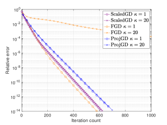
(a) $r=r_{*}=4$

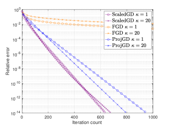
(b) $r=4>r_{*}=2$,

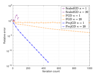
(c) $r=r_{*}=4$

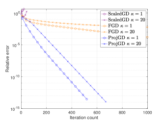
(d) $r=4>r_{*}=2$,

Figure 1: Comparison of ProjGD, FGD, and ScaledGD algorithms for the estimation of asymmetric matrices. Identical step sizes ($\eta=0.4$ in the first row and $\eta=0.6$ in the second row) were employed for all three algorithms, with matrix dimensions set to $n=10$ and ranks of $r_{*}=4$ or $r_{*}=2$. Notably, only ProjGD exhibits consistent linear convergence towards the solution.

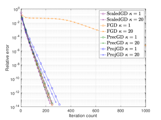
(a) $r=r_{*}=4$

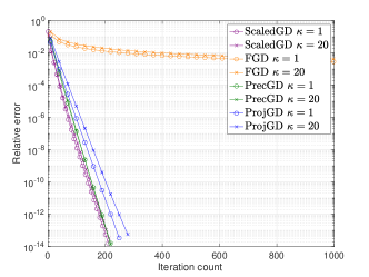
(b) $r=4>r_{*}=2$,

(c) $r=r_{*}=4$

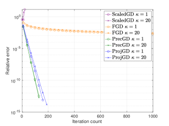
(d) $r=4>r_{*}=2$,

Figure 2: Comparison of ProjGD, FGD, ScaledGD, and PrecGD algorithms for the estimation of positive semidefinite matrices. Identical step sizes ($\eta=0.4$ in the first row and $\eta=0.6$ in the second row) were employed for all three algorithms, with matrix dimensions set to $n=10$ and ranks of $r_{*}=4$ or $r_{*}=2$.

Attentive readers may question the robustness of our comparisons concerning the sensitivity to the chosen step sizes. To address this, we illustrate the convergence speeds of ProjGD, ScaledGD, and FGD under different step sizes $\eta$ (under the first setting as shown in Figure 1(a), with a larger number of observations $m=10nr$). We execute all algorithms for $80$ iterations, ceasing operation if the relative error exceeds $10^{2}$ but remains below $10^{-14}$. This scenario arises when the step size is excessively large, leading to algorithm divergence. Figure 3 plots the relative error with respect to the step size $\eta$ for ProjGD, ScaledGD, and FGD, which shows that ProjGD works well for a large range of step sizes. In particular, when $\eta<0.55$, ProjGD has a similar performance as ScaledGD; and when $0.55<\eta<0.9$, ProjGD still converges while the other two methods diverge. Therefore, our selection of step sizes in previous experiments provides a standard basis for comparing all algorithms.

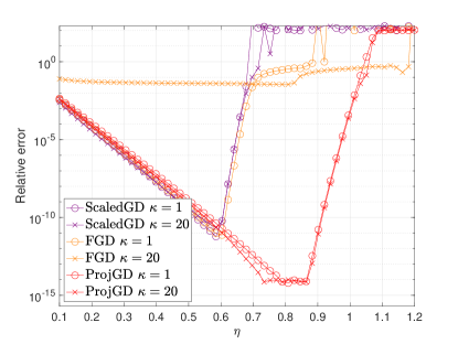
Figure 3: The relative errors of ProjGD, ScaledGD and FGD after 80 iterations with respect to different step sizes $\eta$ from $0.1$ to $1.2$. under different condition numbers $\kappa=1,20$ for matrix sensing with $n=10$, $r=r_{*}=4$, and $m=10nr$.

5 Conclusion

In this work, we investigate the estimation of low-rank matrices employing projected gradient descent, demonstrating its theoretical superiority over factored gradient descent and its variants. As a corollary, we establish that low-rank estimation problems exhibit no local minimizers when the condition number of the objective function is less than $3$. Our future research will explore the non-asymptotic convergence rate and the extension of our anslysis to the estimation of low-rank positive semi-definite matrices.

6 Appendix

6.1 Sketch of Proof of Theorem 1

We first present a few auxiliary lemmas, with their proofs deferred. The first lemma shows that the functional value decreases with each iteration, with the amount of the decrease depending on the changes in the estimation.

Lemma 1 (Decrease in functional value).

Let $\mathbf{X}^{+}=\mathcal{P}_{r}(\mathbf{X}-\eta\nabla f(\mathbf{X}))$, then

$$f(\mathbf{X})-f(\mathbf{X}^{+})\geq\frac{1}{2}\Big{(}\frac{1}{\eta}-L\Big{)}\|\mathbf{X}-\mathbf{X}^{+}\|_{F}^{2}.$$ (12)

Next, we show that the RHS of (12) is bounded by the projection of $\eta\nabla f(\mathbf{X})$ to the subspace $T(\mathbf{X})$:

Lemma 2 (Lower bound of $\|\mathbf{X}-\mathbf{X}^{+}\|_{F}$).

For any $\mathbf{X}\in\mathbb{R}^{n\times n}$ with $\mathrm{rank}(\mathbf{X})=r$ and $\boldsymbol{Y}\in\mathbb{R}^{n\times n}$, we have

$$\|\mathcal{P}_{r}(\boldsymbol{Y})-\mathbf{X}\|_{F}\geq\frac{2}{3}\|P_{T(\mathbf{X})}(\boldsymbol{Y})-\mathbf{X}\|_{F}.$$ (13)

Third, we show that the direction $\mathbf{X}-\mathbf{X}_{*}$ has a large correlation with the subspace $T(\mathbf{X})$, if $\mathbf{X}$ lies in a small neighbor of $\mathbf{X}_{*}$.

Lemma 3 (Local approximation by tangent space).

When $\mathrm{rank}(\mathbf{X}_{*})=r_{*}$ with $r\geq r_{*}$, then for $\mathbf{X}$ such that $\|\mathbf{X}-\mathbf{X}_{*}\|_{F}<c_{0}\sigma_{r_{*}}(\mathbf{X}_{*})$, $\sin\angle(\mathbf{X}-\mathbf{X}_{*},T(\mathbf{X}))\leq\frac{c_{0}}{1-c_{0}}$.

At last, we present a technical lemma that is used in the proof of Lemma 2.

Lemma 4.

Let $\mathbf{X}\in\mathbb{R}^{2n\times 2n}$ with rank $n$ with $\boldsymbol{U}_{\mathbf{X}}\boldsymbol{U}_{\mathbf{X}}^{T}$ and $\mathbf{V}_{\mathbf{X}}\mathbf{V}_{\mathbf{X}}^{T}$ fixed, $\boldsymbol{U},\mathbf{V}\in\mathbb{R}^{2n\times n}$ being orthogonal matrices, then

$$\operatorname*{arg\;min}_{\sigma_{n}(\mathbf{X})\geq 1}\|\mathbf{X}-[\mathbf{X}]_{\boldsymbol{U},\mathbf{V}}\|_{F}\geq\frac{1}{2}\operatorname*{arg\;max}_{\sigma_{1}(\mathbf{X})\leq 1}\|\mathbf{X}-[\mathbf{X}]_{\boldsymbol{U},\mathbf{V}}\|_{F}$$

To prove Theorem 1, we first prove that when $f(\mathbf{X})-f(\mathbf{X}_{*})\leq 0.01\sigma_{r_{*}}(\mathbf{X}_{*})^{2}\mu/\kappa_{f}$, then

$$f(\mathbf{X})-f(\mathbf{X}_{+})\geq c\Big{(}\eta_{T}-\eta_{T}^{2}\Big{)}\frac{\mu}{L}\Big{(}f(\mathbf{X})-f(\mathbf{X}_{*})\Big{)},$$ (14)

where $\mathbf{X}_{+}=\mathcal{P}_{r}\big{(}\mathbf{X}-\eta\nabla f(\mathbf{X})\big{)}$.

Step 1: Proof of (14). We first note that Assumption A1 implies that $f(\mathbf{X})-f(\mathbf{X}_{*})\geq\frac{\mu}{2}\|\mathbf{X}-\mathbf{X}_{*}\|_{F}^{2}$, we have

$$\|\mathbf{X}-\mathbf{X}_{*}\|_{F}\leq\sqrt{2(f(\mathbf{X})-f(\mathbf{X}_{*}))/\mu}\leq\frac{1}{6}\sqrt{\frac{\mu}{L}}\,\sigma_{r_{*}}(\mathbf{X}_{*}),$$ (15)

as a result, Lemma 3 can be applied.

By the Assumption A1 and the estimation that

$$\nabla f(\mathbf{X})-\nabla f(\mathbf{X}_{*})=\int_{t=0}^{1}\nabla^{2}f(\mathbf{X}+t\boldsymbol{\Delta})[\boldsymbol{\Delta}]{\,\mathrm{d}}t$$

where $\boldsymbol{\Delta}=\mathbf{X}-\mathbf{X}_{*}$. Defining $P_{\mathbf{X}}\mathbf{Z}=\frac{\langle\mathbf{X},\mathbf{Z}\rangle}{\|\mathbf{X}\|_{F}^{2}}\mathbf{X}$ as the projection of $\mathbf{Z}$ to the one-dimensional subspace spanned by $\mathbf{X}$, then by Assumption A1, we have

$$f(\mathbf{X})-f(\mathbf{X}_{*})\leq\frac{\|P_{\mathbf{X}-\mathbf{X}_{*}}\nabla f(\mathbf{X})\|_{F}^{2}}{2\mu},$$ (16)

which can be proved by investigating $f$ restricted to the line connecting $\mathbf{X}$ and $\mathbf{X}_{*}$.Similarly, we have

$$f(\mathbf{X})-f(\mathbf{X}_{*})\geq\frac{\|\nabla f(\mathbf{X})\|_{F}^{2}}{2L},$$ (17)

Now let us investigate $\|P_{T(\mathbf{X})}\nabla f(\mathbf{X})\|_{F}$. Decompose $\nabla f(\mathbf{X})=\mathbf{Z}_{1}+\mathbf{Z}_{2}$, where $\mathbf{Z}_{1}=P_{\mathbf{X}-\mathbf{X}_{*}}\nabla f(\mathbf{X})$ is the projection to the direction $\mathbf{X}-\mathbf{X}_{*}$ and $\mathbf{Z}_{2}$ is the reminder. In addition, let $\boldsymbol{Y}=P_{T(\mathbf{X})}(\mathbf{X}-\mathbf{X}_{*})$, then Lemma 3 implies that $\sin\angle(\boldsymbol{Y},\mathbf{X}-\mathbf{X}_{*})<\|\mathbf{X}-\mathbf{X}_{*}\|_{F}/\sigma_{r_{*}}(\mathbf{X}_{*})$. As $\mathbf{Z}_{2}$ is orthogonal to $\mathbf{X}-\mathbf{X}_{*}$, we have

$$\|P_{\boldsymbol{Y}}\mathbf{Z}_{2}\|_{F}\leq\frac{\|\mathbf{X}-\mathbf{X}_{*}\|_{F}}{\sigma_{r_{*}}(\mathbf{X}_{*})}\|\mathbf{Z}_{2}\|_{F}\leq\frac{\|\mathbf{X}-\mathbf{X}_{*}\|_{F}}{\sigma_{r_{*}}(\mathbf{X}_{*})}\sqrt{2L(f(\mathbf{X})-f(\mathbf{X}_{*}))},$$ (18)

where the last step follows from (17). In addition,

$$\|P_{\boldsymbol{Y}}\mathbf{Z}_{1}\|_{F}\geq\frac{1}{2}\|\mathbf{Z}_{1}\|_{F}\geq\frac{1}{2}\sqrt{2\mu(f(\mathbf{X})-f(\mathbf{X}_{*}))},$$ (19)

where the last step follows from (16). Combining (18) and (19), we have

$$\|P_{T(\mathbf{X})}\nabla f(\mathbf{X})\|_{F}\geq\|P_{\boldsymbol{Y}}(\mathbf{Z}_{1}+\mathbf{Z}_{2})\|_{F}\geq\|P_{\boldsymbol{Y}}\mathbf{Z}_{1}\|_{F}-\|P_{\boldsymbol{Y}}\mathbf{Z}_{2}\|_{F}$$ (20)

$$\geq {\sqrt{2(f(\mathbf{X})-f(\mathbf{X}_{*}))}}\Big{(}\frac{\sqrt{\mu}}{2}-\frac{\|\mathbf{X}-\mathbf{X}_{*}\|_{F}}{\sigma_{r_{*}}(\mathbf{X}_{*})}\sqrt{L}\Big{)}.$$

Combining the Lemmas and the estimations above, we have

$$f(\mathbf{X})-f(\mathbf{X}^{+})\geq\frac{1}{2}\Big{(}\frac{1}{\eta}-L\Big{)}\|\mathbf{X}-\mathbf{X}^{+}\|_{F}^{2}\geq\frac{2}{9}\Big{(}\frac{1}{\eta}-L\Big{)}\eta^{2}\|P_{T(\mathbf{X})}\nabla f(\mathbf{X})\|_{F}^{2}$$ (21)

$$\geq \frac{2}{9}\Big{(}\frac{1}{\eta}-L\Big{)}\eta^{2}{{2(f(\mathbf{X})-f(\mathbf{X}_{*}))}}\Big{(}\frac{\sqrt{\mu}}{2}-\frac{\|\mathbf{X}-\mathbf{X}_{*}\|_{F}}{\sigma_{r_{*}}(\mathbf{X}_{*})}\sqrt{L}\Big{)}^{2}$$

$$\geq \frac{2}{9}\Big{(}\frac{1}{\eta}-L\Big{)}\eta^{2}{{2(f(\mathbf{X})-f(\mathbf{X}_{*}))}}\Big{(}\frac{\sqrt{\mu}}{3}\Big{)}^{2}$$

$$= \frac{4\mu}{27}\Big{(}\frac{1}{\eta}-L\Big{)}\eta^{2}{{(f(\mathbf{X})-f(\mathbf{X}_{*}))}}$$

where the first inequality follows from Lemma 1, the second inequality follows from Lemma 2, the third inequality follows from (20), and the last inequality follows from (15).

Step 2: Proof of Theorem. It is sufficient to show that (14) holds over each iteration where $\mathbf{X}$ and $\mathbf{X}_{*}$ are replaced with $\mathbf{X}^{(k)}$ and $\mathbf{X}^{(k+1)}$. The proof is based on induction: assume that (14) holds when $\mathbf{X}$ is replaced with $\mathbf{X}^{(0)},\cdots,\mathbf{X}^{(k-1)}$, then we have $f(\mathbf{X}^{(k)})\leq f(\mathbf{X}^{(0)})$ as this assumption means that the objective value is nonincreasing in the first $k$ iterations. As a result, the assumption and the proof of (14) still hold when $\mathbf{X}$ and $\mathbf{X}_{*}$ are replaced with $\mathbf{X}^{(k)}$ and $\mathbf{X}^{(k+1)}$. As a result, (14) holds for all iterations and the Theorem is proved.

6.1.1 Proof of Lemmas

Proof of Lemma 1.

Note that the fundamental theorem of calculus implies

$$f(\mathbf{X})-f(\mathbf{X}^{+})-\langle\nabla f(\mathbf{X}),\mathbf{X}-\mathbf{X}^{+}\rangle+\int_{t=0}^{1}\langle\nabla f(\mathbf{X}(t))-\nabla f(\mathbf{X}),\mathbf{X}-\mathbf{X}_{+}\rangle{\,\mathrm{d}}t=0$$

where

$$\langle\nabla f(\mathbf{X}(t))-\nabla f(\mathbf{X}),\mathbf{X}-\mathbf{X}_{+}\rangle=\int_{u=0}^{t}\langle\nabla^{2}f(\mathbf{X}(u))[\mathbf{X}-\mathbf{X}_{+}],\mathbf{X}-\mathbf{X}_{+}\rangle{\,\mathrm{d}}u.$$

Since $\|\mathbf{X}^{+}-(\mathbf{X}-\eta\nabla f(\mathbf{X}))\|_{F}\leq\|\mathbf{X}-(\mathbf{X}-\eta\nabla f(\mathbf{X}))\|_{F}$, we have

$$\langle\eta\nabla f(\mathbf{X}),\mathbf{X}-\mathbf{X}^{+}\rangle\geq\frac{1}{2}\|\mathbf{X}-\mathbf{X}^{+}\|_{F}^{2}.$$ (22)

Combining it with the property (4) that

$$\Big{|}\langle\nabla^{2}f(\mathbf{X}(u))[\mathbf{X}-\mathbf{X}_{+}],\mathbf{X}-\mathbf{X}_{+}\rangle\Big{|}\leq L\|\mathbf{X}-\mathbf{X}^{+}\|_{F}^{2},$$

we have (12) and Lemma 1 is proved. ∎

Proof of Lemma 2.

First, we will prove Lemma 2 for the setting

$$[\mathcal{P}_{r}(\boldsymbol{Y})]_{\boldsymbol{U}_{\mathbf{X}},\mathbf{V}_{\mathbf{X}}}=\mathbf{X}.$$ (23)

Then

$$\mathcal{P}_{r}(\boldsymbol{Y})-\mathbf{X}=\mathcal{P}_{r}(\boldsymbol{Y})-[\mathcal{P}_{r}(\boldsymbol{Y})]_{\boldsymbol{U}_{\mathbf{X}},\mathbf{V}_{\mathbf{X}}},$$ (24)

and

$$\|P_{T(\mathbf{X})}(\boldsymbol{Y})-\mathbf{X}\|_{F}\leq \|P_{T(\mathbf{X})}(\mathcal{P}_{r}(\boldsymbol{Y}))-\mathbf{X}\|_{F}+\|P_{T(\mathbf{X})}(\boldsymbol{Y}-\mathcal{P}_{r}(\boldsymbol{Y}))\|_{F}$$

$$= \|P_{T(\mathbf{X})}(\mathcal{P}_{r}(\boldsymbol{Y})-\mathbf{X})\|_{F}+\|(\boldsymbol{Y}-\mathcal{P}_{r}(\boldsymbol{Y}))-[(\boldsymbol{Y}-\mathcal{P}_{r}(\boldsymbol{Y}))]_{\boldsymbol{U}_{\mathbf{X},\perp},\mathbf{V}_{\mathbf{X},\perp}}\|_{F}.$$ (25)

Note that $\boldsymbol{U}_{\mathcal{P}_{r}(\boldsymbol{Y}),\perp}=\boldsymbol{U}_{\boldsymbol{Y}-\mathcal{P}_{r}(\boldsymbol{Y})}$ and $\mathbf{V}_{\mathcal{P}_{r}(\boldsymbol{Y}),\perp}=\mathbf{V}_{\boldsymbol{Y}-\mathcal{P}_{r}(\boldsymbol{Y})}$, so Lemma 4 can be applied to show that

$$\|(\boldsymbol{Y}-\mathcal{P}_{r}(\boldsymbol{Y}))-[(\boldsymbol{Y}-\mathcal{P}_{r}(\boldsymbol{Y}))]_{\boldsymbol{U}_{\mathbf{X},\perp},\mathbf{V}_{\mathbf{X},\perp}}\|_{F}\leq\frac{1}{2}\|\mathcal{P}_{r}(\boldsymbol{Y})-[\mathcal{P}_{r}(\boldsymbol{Y})]_{\boldsymbol{U}_{\mathbf{X}},\mathbf{V}_{\mathbf{X}}}\|_{F}=\frac{1}{2}\|\mathcal{P}_{r}(\boldsymbol{Y})-\mathbf{X}\|_{F},$$ (26)

where the last step follows form (24).

On the other hand, we have

$$\|P_{T(\mathbf{X})}(\mathcal{P}_{r}(\boldsymbol{Y})-\mathbf{X})\|_{F}\leq\|\mathcal{P}_{r}(\boldsymbol{Y})-\mathbf{X})\|_{F}.$$

Combining it with (25) and (26), Lemma 2 is proved under assumption (23).

It remains to prove Lemma 2 without assumption (23). Let $\mathbf{X}^{\prime}$ be defined by

$$\mathbf{X}^{\prime}=[\mathcal{P}_{r}(\boldsymbol{Y})]_{\boldsymbol{U}_{\mathbf{X}},\mathbf{V}_{\mathbf{X}}},$$

then from the previous analysis we have

$$\|\mathcal{P}_{r}(\boldsymbol{Y})-\mathbf{X}^{\prime}\|_{F}\geq\frac{2}{3}\|P_{T(\mathbf{X})}(\boldsymbol{Y})-\mathbf{X}^{\prime}\|_{F}.$$ (27)

Combining it with

$$\|\mathcal{P}_{r}(\boldsymbol{Y})-\mathbf{X}\|_{F}^{2}=\|\mathcal{P}_{r}(\boldsymbol{Y})-\mathbf{X}^{\prime}\|_{F}^{2}+\|\mathbf{X}-\mathbf{X}^{\prime}\|_{F}^{2}\geq(\|\mathcal{P}_{r}(\boldsymbol{Y})-\mathbf{X}^{\prime}\|_{F}+\|\mathbf{X}-\mathbf{X}^{\prime}\|_{F})^{2}/2,$$

and

$$\|P_{T(\mathbf{X})}(\boldsymbol{Y})-\mathbf{X}\|_{F}\leq\|P_{T(\mathbf{X})}(\boldsymbol{Y})-\mathbf{X}^{\prime}\|_{F}+\|\mathbf{X}-\mathbf{X}^{\prime}\|_{F},$$

equation (13) and Lemma 2 are proved. ∎

Proof of Lemma 4.

Let $\sigma^{(1)}_{i}$ be the singular values of $\boldsymbol{U}^{T}\boldsymbol{U}_{\mathbf{X}}$ and $\sigma^{(2)}_{i}$ be the singular values of $\mathbf{V}^{T}\mathbf{V}_{\mathbf{X}}$, then it is equivalent to prove that for $\Sigma_{ij}=1-\sigma^{(1)}_{i}\sigma^{(2)}_{j}$,

$$\operatorname*{arg\;min}_{\sigma_{n}(\mathbf{X})\geq 1}\|\mathbf{X}\circ\Sigma\|_{F}\geq c\operatorname*{arg\;max}_{\sigma_{1}(\mathbf{X})\leq 1}\|\mathbf{X}\circ\Sigma\|_{F}.$$ (28)

Note that the minimizers and the maximizers of (28) are achieved at the boundary of the constraint set, i.e., when $\mathbf{X}$ is an orthogonal matrix, that is

$$\operatorname*{arg\;min}_{\sigma_{n}(\mathbf{X})\geq 1}\|\mathbf{X}\circ\Sigma\|_{F}=\operatorname*{arg\;min}_{\mathbf{X}\mathbf{X}^{T}=\mathbf{I}}\|\mathbf{X}\circ\Sigma\|_{F},\,\,\,\,\,\,\operatorname*{arg\;max}_{\sigma_{1}(\mathbf{X})\leq 1}\|\mathbf{X}\circ\Sigma\|_{F}=\operatorname*{arg\;max}_{\mathbf{X}\mathbf{X}^{T}=\mathbf{I}}\|\mathbf{X}\circ\Sigma\|_{F}.$$ (29)

Let $\tau^{(k)}_{i}=1-\sigma^{(k)}_{i}$, then $(\tau^{(1)\,2}_{i}+\tau^{(2\,2)}_{j})/2\leq\Sigma_{ij}^{2}\leq 2(\tau^{(1)\,2}_{i}+\tau^{(2\,2)}_{j})$, and we have

$$\|\mathbf{X}\circ\Sigma\|_{F}^{2}\leq 2\sum_{i,j}\mathbf{X}_{ij}^{2}(\tau^{(1)\,2}_{i}+\tau^{(2\,2)}_{j})=2\sum_{i}\tau^{(1)\,2}_{i}+\sum_{j}\tau^{(2)\,2}_{j}$$

and

$$\|\mathbf{X}\circ\Sigma\|_{F}^{2}\geq\frac{1}{2}\sum_{i,j}\mathbf{X}_{ij}^{2}(\tau^{(1)\,2}_{i}+\tau^{(2\,2)}_{j})=\geq\frac{1}{2}\sum_{i}\tau^{(1)\,2}_{i}+\sum_{j}\tau^{(2)\,2}_{j}.$$

Combing the estimations above with (29), the Lemma 4 is proved.

∎

Proof of Lemma 3.

Note that

$$\|P_{T(\mathbf{X})^{\perp}}(\mathbf{X}-\mathbf{X}_{*})\|_{F}=\|[\mathbf{X}-\mathbf{X}_{*}]_{\boldsymbol{U}_{\mathbf{X}}^{\perp},\mathbf{V}_{\mathbf{X}}^{\perp}}\|_{F}$$

$$= \|[\mathbf{X}-\mathbf{X}_{*}]_{\boldsymbol{U}_{\mathbf{X}}^{\perp},\mathbf{V}_{\mathbf{X}}}(\mathbf{X}-[\mathbf{X}-\mathbf{X}_{*}]_{\boldsymbol{U}_{\mathbf{X}},\mathbf{V}_{\mathbf{X}}})^{-1}[\mathbf{X}-\mathbf{X}_{*}]_{\boldsymbol{U}_{\mathbf{X}},\mathbf{V}_{\mathbf{X}}^{\perp}}\|_{F}$$

$$\leq \frac{\|[\mathbf{X}-\mathbf{X}_{*}]\|_{F}^{2}}{\sigma_{r_{*}}(\mathbf{X})-\|[\mathbf{X}-\mathbf{X}_{*}\|_{F}}.$$

Then the lemma is proved.

∎

6.2 Proof of Theorem 2

Without loss of generality, let us assume $(L+\mu)/2=1$. Consequently, we have $\kappa_{0}=L-1=1-\mu$, and the condition $L/\mu<3$ ensures that $\kappa_{0}\leq 1/2$.

Moreover, by selecting $\epsilon$ in part (b) to approach zero, we can ensure that $\hat{\kappa}_{0}$ closely approximates $\kappa_{0}$ and remains smaller than $\eta_{0}$. Hence, according to Theorem 2(b), part (a) naturally follows. Subsequently, the remainder of the proof focuses on establishing the validity of part (b).

To prove part(b), we first present a few auxiliary lemmas, with their proofs deferred.

Lemma 5 (Bound on derivative).

$$\|\nabla f(\mathbf{X})-(\mathbf{X}-\mathbf{X}_{*})\|_{F}\leq\kappa_{0}\|\mathbf{X}-\mathbf{X}_{*}\|_{F}.$$ (30)

Lemma 6 (Change over iterations).

We have

$$\|\mathcal{P}_{r}(\mathbf{X}+\mathbf{Z})-\mathbf{X}\|_{F}\geq\max\Big{(}\frac{1}{2}(\|\mathbf{Z}\|-\sigma_{r}(\mathbf{X})),\frac{2}{3}\|P_{T(\mathbf{X})}(\mathbf{Z})\|_{F}\Big{)}$$

Lemma 7 (Property of stationary points).

Assuming that $P_{T(\mathbf{X})}\mathbf{Z}=0$ and

$$\|\mathbf{Z}-(\mathbf{X}_{*}-\mathbf{X})\|_{F}\leq\kappa_{0}\|\mathbf{X}-\mathbf{X}_{*}\|_{F},\,\,$$ (31)

then we have $\|P_{T(\mathbf{X})^{\perp}}\mathbf{Z}\|\geq\frac{{1-\kappa_{0}^{2}}}{\kappa_{0}}\sigma_{r}(\mathbf{X})$.

Lemma 8 (Auxiliary result on matrix inequalities).

For matrices $\mathbf{X},\boldsymbol{Y}\in\mathbb{R}^{n\times n}$ and orthogonal matrices $\boldsymbol{U},\mathbf{V}\in\mathbb{R}^{n\times n}$,

$$\mathrm{tr}(\boldsymbol{U}\mathbf{X}\mathbf{V}\boldsymbol{Y})\leq\sum_{i=1}^{n}\sigma_{i}(\mathbf{X})\sigma_{i}(\boldsymbol{Y}),$$

with equality achieved when $\mathbf{X}$ and $\boldsymbol{Y}$ are both diagonal matrices with diagonal entries nonincreasing.

Let $\mathbf{Z}=-\nabla f(\mathbf{X})$, then By Lemma 5, we have

$$\Big{\|}P_{T(\mathbf{X})}(\mathbf{Z}-(\mathbf{X}_{*}-\mathbf{X}))\Big{\|}_{F}^{2}+\Big{\|}P_{T(\mathbf{X})^{\perp}}(\mathbf{Z}-(\mathbf{X}_{*}-\mathbf{X}))\Big{\|}_{F}^{2}$$ (32)

$$\leq \kappa_{0}^{2}\Big{(}\Big{\|}P_{T(\mathbf{X})}(\mathbf{X}_{*}-\mathbf{X})\Big{\|}_{F}^{2}+\Big{\|}P_{T(\mathbf{X})^{\perp}}(\mathbf{X}_{*}-\mathbf{X})\Big{\|}_{F}^{2}\Big{)}.$$

Assuming $\|P_{T(\mathbf{X})}\mathbf{Z}\|_{F}=\gamma,$ then $\|P_{T(\mathbf{X})}(\mathbf{Z}-(\mathbf{X}_{*}-\mathbf{X}))\|_{F}\geq\|P_{T(\mathbf{X})}(\mathbf{X}_{*}-\mathbf{X})\|_{F}-\gamma$ and

$$\Big{\|}P_{T(\mathbf{X})^{\perp}}(\mathbf{Z})-P_{T(\mathbf{X})^{\perp}}(\mathbf{X}_{*})\Big{\|}_{F}^{2}=\Big{\|}P_{T(\mathbf{X})^{\perp}}(\mathbf{Z}-(\mathbf{X}_{*}-\mathbf{X}))\Big{\|}_{F}^{2}$$

$$\leq \kappa_{0}^{2}\Big{(}\Big{\|}P_{T(\mathbf{X})}(\mathbf{X}_{*}-\mathbf{X})\Big{\|}_{F}^{2}+\Big{\|}P_{T(\mathbf{X})^{\perp}}(\mathbf{X}_{*}-\mathbf{X})\Big{\|}_{F}^{2}\Big{)}-\Big{(}\Big{\|}P_{T(\mathbf{X})}(\mathbf{X}_{*}-\mathbf{X})\Big{\|}_{F}-\gamma\Big{)}^{2}$$

$$= \Bigg{(}\kappa_{0}^{2}\Big{\|}P_{T(\mathbf{X})}(\mathbf{X}_{*}-\mathbf{X})\Big{\|}_{F}^{2}-\Big{(}\Big{\|}P_{T(\mathbf{X})}(\mathbf{X}_{*}-\mathbf{X})\Big{\|}_{F}-\gamma\Big{)}^{2}\Bigg{)}+\kappa_{0}^{2}\Big{\|}P_{T(\mathbf{X})^{\perp}}\mathbf{X}_{*}\Big{\|}_{F}^{2}$$ (33)

Next, we will investigate the bound of $\|\mathcal{P}_{r}(\mathbf{X}+\eta\mathbf{Z})-\mathbf{X}\|_{F}/\|\mathbf{X}-\mathbf{X}_{*}\|_{F}$ in two cases.

Case 1: $\|P_{T(\mathbf{X})^{\perp}}(\mathbf{X}_{*})\|_{F}/\|\mathbf{X}-\mathbf{X}_{*}\|_{F}\geq\sqrt{2}/2$.
Since $\|P_{T(\mathbf{X})^{\perp}}(\mathbf{X}_{*})\|_{F}=\|P_{T(\mathbf{X})^{\perp}}(\mathbf{X}-\mathbf{X}_{*})\|_{F}$ and $\|\mathbf{X}-\mathbf{X}_{*}\|_{F}^{2}=\|P_{T(\mathbf{X})}(\mathbf{X}-\mathbf{X}_{*})\|_{F}^{2}+\|P_{T(\mathbf{X})^{\perp}}(\mathbf{X}-\mathbf{X}_{*})\|_{F}^{2}$, the assumption implies that

$$P_{T(\mathbf{X})}(\mathbf{X}-\mathbf{X}_{*})\|_{F}\leq\|P_{T(\mathbf{X})^{\perp}}(\mathbf{X}_{*})\|_{F}.$$ (34)

Case 1a: If $\gamma\leq\epsilon\|\mathbf{X}-\mathbf{X}_{*}\|_{F}$, then by assumption $\gamma\leq 2\epsilon\|P_{T(\mathbf{X})^{\perp}}(\mathbf{X}-\mathbf{X}_{*})\|_{F}$, so the RHS of (33) is bounded by

$$P_{T(\mathbf{X})}(\mathbf{X}_{*}-\mathbf{X})(\kappa_{0}^{2}-(1-2\epsilon)^{2})\Big{\|}P_{T(\mathbf{X})}(\mathbf{X}_{*}-\mathbf{X})\Big{\|}_{F}^{2}+\kappa_{0}^{2}\Big{\|}P_{T(\mathbf{X})^{\perp}}\mathbf{X}_{*}\Big{\|}_{F}^{2}$$

$$\leq (\hat{\kappa}_{0}^{2}-1)\Big{\|}P_{T(\mathbf{X})}(\mathbf{X}_{*}-\mathbf{X})\Big{\|}_{F}^{2}+\hat{\kappa}_{0}^{2}\Big{\|}P_{T(\mathbf{X})^{\perp}}\mathbf{X}_{*}\Big{\|}_{F}^{2}$$

where the last step applied (34) and assumes that $\hat{\kappa}_{0}^{2}={\kappa}_{0}^{2}+2\epsilon-2\epsilon^{2}$. This and (33) implies that

$$\|P_{T(\mathbf{X})^{\perp}}\mathbf{Z}-(\mathbf{X}_{*}-\mathbf{X})\|_{F}\leq\hat{\kappa}_{0}\|\mathbf{X}-\mathbf{X}_{*}\|_{F},\,\,$$ (35)

that is, (31) holds when $\mathbf{Z}$ is replaced with $P_{T(\mathbf{X})^{\perp}}\mathbf{Z}$ and $\kappa_{0}$ is replaced with $\hat{\kappa}_{0}$.

Choose $\epsilon$ small such that $\hat{\kappa}_{0}<1/2$, then Lemma 7 implies $\|P_{T(\mathbf{X})^{\perp}}\mathbf{Z}\|\geq\frac{{1-\hat{\kappa}_{0}^{2}}}{\hat{\kappa}_{0}}\sigma_{r}(\mathbf{X})$, so for $\eta>\frac{\hat{\kappa}_{0}}{{1-\hat{\kappa}_{0}^{2}}}$,

$$\eta\|P_{T(\mathbf{X})^{\perp}}\mathbf{Z}\|-\sigma_{r}(\mathbf{X})\geq\Big{(}\eta-\frac{\hat{\kappa}_{0}}{{1-\hat{\kappa}_{0}^{2}}}\Big{)}\|P_{T(\mathbf{X})^{\perp}}\mathbf{Z}\|.$$

On the other hand, (31) implies that

$$\|P_{T(\mathbf{X})^{\perp}}\mathbf{Z}\|_{F}\geq\|P_{T(\mathbf{X})^{\perp}}(\mathbf{X}-\mathbf{X}_{*})\|_{F}-\kappa_{0}\|\mathbf{X}-\mathbf{X}_{*}\|_{F}\geq(\sqrt{2}/2-\kappa_{0})\|\mathbf{X}-\mathbf{X}_{*}\|_{F},$$

so $\|P_{T(\mathbf{X})^{\perp}}\mathbf{Z}\|\geq\frac{1}{\sqrt{r}}(\sqrt{2}/2-\kappa_{0})\|\mathbf{X}-\mathbf{X}_{*}\|_{F}$ (note tha $\mathrm{rank}(P_{T(\mathbf{X})^{\perp}}\mathbf{Z})\leq r$) and

$$\eta\|P_{T(\mathbf{X})^{\perp}}\mathbf{Z}\|-\sigma_{r}(\mathbf{X})\geq\frac{1}{\sqrt{r}}\Big{(}\eta-\frac{\hat{\kappa}_{0}}{{1-\hat{\kappa}_{0}^{2}}}\Big{)}\Big{(}\frac{\sqrt{2}}{2}-{\kappa}_{0}\Big{)}\|\mathbf{X}-\mathbf{X}_{*}\|_{F}.$$

Combining it with Lemma 6, we have

$$\|\mathcal{P}_{r}(\mathbf{X}+\eta\mathbf{Z})-\mathbf{X}\|_{F}\geq\frac{1}{2\sqrt{r}}\Big{(}\eta-\frac{\hat{\kappa}_{0}}{{1-\hat{\kappa}_{0}^{2}}}\Big{)}\Big{(}\frac{\sqrt{2}}{2}-{\kappa}_{0}\Big{)}\|\mathbf{X}-\mathbf{X}_{*}\|_{F}.$$ (36)

Case 1b: When $\gamma>\epsilon\|\mathbf{X}-\mathbf{X}_{*}\|_{F}$, Lemma 6 implies that

$$\Big{\|}\mathcal{P}_{r}(\mathbf{X}+\eta\mathbf{Z})-\mathbf{X}\Big{\|}_{F}\geq\frac{2}{3}\Big{\|}\eta P_{T(\mathbf{X})}(\mathbf{Z})\Big{\|}_{F}\geq\frac{2}{3}\epsilon\eta\Big{\|}\mathbf{X}-\mathbf{X}_{*}\Big{\|}_{F}.$$ (37)

Case 2: $\|P_{T(\mathbf{X})^{\perp}}(\mathbf{X}_{*})\|_{F}/\|\mathbf{X}-\mathbf{X}_{*}\|_{F}<\sqrt{2}/2$
Then following a similar argument as (34), we have

$$P_{T(\mathbf{X})}(\mathbf{X}-\mathbf{X}_{*})\|_{F}\geq\frac{\sqrt{2}}{2}\|\mathbf{X}-\mathbf{X}_{*}\|_{F}.$$ (38)

In addition, (31) implies that

$$\|P_{T(\mathbf{X})}\mathbf{Z}-P_{T(\mathbf{X})}(\mathbf{X}_{*}-\mathbf{X})\|_{F}\leq\kappa_{0}\|\mathbf{X}-\mathbf{X}_{*}\|_{F}.$$

Combining it with (38), we have

$$\|P_{T(\mathbf{X})}\mathbf{Z}\|_{F}\geq\Big{(}\frac{\sqrt{2}}{2}-\kappa_{0}\Big{)}\|\mathbf{X}-\mathbf{X}_{*}\|_{F}.$$

Combining it with Lemma 2, we have

$$\|\mathcal{P}_{r}(\mathbf{X}+\eta\mathbf{Z})-\mathbf{X}\|_{F}>\eta\frac{2}{3}\Big{(}\frac{\sqrt{2}}{2}-\kappa_{0}\Big{)}\|\mathbf{X}-\mathbf{X}_{*}\|_{F}>\eta\frac{1}{10}\|\mathbf{X}-\mathbf{X}_{*}\|_{F}.$$ (39)

Summary Combining (36), (37), (39) and Lemma 1, we have

$$f(\mathbf{X}_{+})-f(\mathbf{X})\geq\frac{1}{2}\Big{(}\frac{1}{\eta}-L\Big{)}\min\Bigg{(}\frac{\eta}{10},\frac{2\epsilon\eta}{3},\frac{1}{2\sqrt{r}}\Big{(}\eta-\frac{\hat{\kappa}_{0}}{{1-\hat{\kappa}_{0}^{2}}}\Big{)}\Bigg{)}^{2}\|\mathbf{X}-\mathbf{X}_{*}\|_{F}^{2}$$

$$\geq \frac{1}{L}\Big{(}\frac{1}{\eta}-L\Big{)}\min\Bigg{(}\frac{\eta}{10},\frac{2\epsilon\eta}{3},\frac{1}{2\sqrt{r}}\Big{(}\eta-\frac{\hat{\kappa}_{0}}{{1-\hat{\kappa}_{0}^{2}}}\Big{)}\Bigg{)}^{2}(f(\mathbf{X})-f(\mathbf{X}_{*})),$$

where the last step follows from Assumption A1 such that $\|\mathbf{X}-\mathbf{X}_{*}\|_{F}^{2}\geq 2(f(\mathbf{X})-f(\mathbf{X}_{*}))/L$. Since $\eta L=\eta_{0}(1+\kappa_{0})$. the theorem is proved.

6.2.1 Proof of Lemmas

Proof of Lemma 5.

Recall Assumption A1 that

$$\|\nabla^{2}f(\mathbf{X})[\boldsymbol{E}]-\boldsymbol{E}\|_{F}\leq\kappa_{0}\|\boldsymbol{E}\|_{F},$$

let $\boldsymbol{E}=\mathbf{X}-\mathbf{X}_{*}$ and $\mathbf{X}(t)=\mathbf{X}_{*}+t\boldsymbol{E}$ be the parameterization of the line connecting $\mathbf{X}$ and $\mathbf{X}_{*}$, then

$$\Big{\|}\Big{(}\nabla f(\mathbf{X})-\nabla f(\mathbf{X}_{*})\Big{)}-(\mathbf{X}-\mathbf{X}_{*})\Big{\|}_{F}=\Big{\|}\int_{t=0}^{1}\Big{(}\nabla^{2}f(\mathbf{X}(t))[\boldsymbol{E}]-\boldsymbol{E}\Big{)}{\,\mathrm{d}}t\Big{\|}_{F}\leq\kappa_{0}\|\mathbf{X}-\mathbf{X}_{*}\|_{F}.$$

Note that $\nabla f(\mathbf{X}_{*})=0$, Lemma 5 is proved. ∎

Proof of Lemma 6.

The part $\|\mathcal{P}_{r}(\mathbf{X}+\mathbf{Z})-\mathbf{X}\|_{F}\geq\frac{2}{3}\|P_{T(\mathbf{X})}(\mathbf{Z})\|_{F}$ follows from Lemma 2.

On the other hand,

$$\sigma_{r+1}(\mathcal{P}_{r}(\mathbf{X}+\mathbf{Z}))=\|(\mathbf{X}+\mathbf{Z})-\mathcal{P}_{r}(\mathbf{X}+\mathbf{Z})\|\geq\|\mathbf{Z}\|-\|\mathcal{P}_{r}(\mathbf{X}+\mathbf{Z})-\mathbf{X}\|$$

and

$$\sigma_{r}(\mathcal{P}_{r}(\mathbf{X}+\mathbf{Z}))\leq\sigma_{r}(\mathbf{X})+\|\mathcal{P}_{r}(\mathbf{X}+\mathbf{Z})-\mathbf{X}\|,$$

so

$$\|\mathcal{P}_{r}(\mathbf{X}+\mathbf{Z})-\mathbf{X}\|\geq\frac{1}{2}(\|\mathbf{Z}\|-\sigma_{r}(\mathbf{X})).$$

∎

Proof of Lemma 7.

Step 1 In this step, we claim that

$$\Big{\|}P_{T(\mathbf{X})}(\mathbf{X}_{*})-\mathbf{X}\Big{\|}_{F}^{2}\leq\sum_{i=1}^{r}\big{(}\sigma_{i}([\mathbf{X}_{*}]_{\boldsymbol{U}_{\mathbf{X}},\mathbf{V}_{\mathbf{X}}})-\sigma_{i}(\mathbf{X})\big{)}^{2}+2{\sum_{i=1}^{r}\sigma_{i}(\mathbf{X})\sigma_{r+1-i}(P_{T(\mathbf{X})^{\perp}}(\mathbf{X}_{*}))}.$$ (40)

Write

$$\mathbf{X}_{*}=\begin{pmatrix}[\mathbf{X}_{*}]_{\boldsymbol{U}_{\mathbf{X}},\mathbf{V}_{\mathbf{X}}}&[\mathbf{X}_{*}]_{\boldsymbol{U}_{\mathbf{X}},\mathbf{V}_{\mathbf{X}}^{\perp}}\\ [\mathbf{X}_{*}]_{\boldsymbol{U}_{\mathbf{X}}^{\perp},\mathbf{V}_{\mathbf{X}}}&[\mathbf{X}_{*}]_{\boldsymbol{U}_{\mathbf{X}}^{\perp},\mathbf{V}_{\mathbf{X}}^{\perp}}\end{pmatrix},$$

then

$$\|P_{T(\mathbf{X})}(\mathbf{X}_{*})-\mathbf{X}\|_{F}^{2}=\|[\mathbf{X}_{*}]_{\boldsymbol{U}_{\mathbf{X}}^{\perp},\mathbf{V}_{\mathbf{X}}}\|_{F}^{2}+\|[\mathbf{X}_{*}]_{\boldsymbol{U}_{\mathbf{X}},\mathbf{V}_{\mathbf{X}}^{\perp}}\|_{F}^{2}+\|[\mathbf{X}_{*}]_{\boldsymbol{U}_{\mathbf{X}},\mathbf{V}_{\mathbf{X}}}-\mathbf{X}\|_{F}^{2}.$$ (41)

To minimize the RHS of (41), we apply Lemma 8.

1. Upper bound of $\|[\mathbf{X}_{*}]_{\boldsymbol{U}_{\mathbf{X}}^{\perp},\mathbf{V}_{\mathbf{X}}}\|_{F}^{2}+\|[\mathbf{X}_{*}]_{\boldsymbol{U}_{\mathbf{X}},\mathbf{V}_{\mathbf{X}}^{\perp}}\|_{F}^{2}$

Assuming that $[\mathbf{X}_{*}]_{\boldsymbol{U}_{\mathbf{X}}^{\perp},\mathbf{V}_{\mathbf{X}}}=\boldsymbol{Y}[\mathbf{X}_{*}]_{\boldsymbol{U}_{\mathbf{X}},\mathbf{V}_{\mathbf{X}}}$, then $\mathrm{rank}(\mathbf{X})=n$ implies $[\mathbf{X}_{*}]_{\boldsymbol{U}_{\mathbf{X}}^{\perp},\mathbf{V}_{\mathbf{X}}^{\perp}}=\boldsymbol{Y}[\mathbf{X}_{*}]_{\boldsymbol{U}_{\mathbf{X}},\mathbf{V}_{\mathbf{X}}^{\perp}}$, that is, $[\mathbf{X}_{*}]_{\boldsymbol{U}_{\mathbf{X}},\mathbf{V}_{\mathbf{X}}^{\perp}}=\boldsymbol{Y}^{-1}[\mathbf{X}_{*}]_{\boldsymbol{U}_{\mathbf{X}}^{\perp},\mathbf{V}_{\mathbf{X}}^{\perp}}$.

Then

$$\|[\mathbf{X}_{*}]_{\boldsymbol{U}_{\mathbf{X}}^{\perp},\mathbf{V}_{\mathbf{X}}}\|_{F}^{2}=\|\boldsymbol{Y}[\mathbf{X}_{*}]_{\boldsymbol{U}_{\mathbf{X}},\mathbf{V}_{\mathbf{X}}}\|_{F}^{2}=\langle[\mathbf{X}_{*}]_{\boldsymbol{U}_{\mathbf{X}},\mathbf{V}_{\mathbf{X}}}[\mathbf{X}_{*}]_{\boldsymbol{U}_{\mathbf{X}},\mathbf{V}_{\mathbf{X}}}^{T},\boldsymbol{Y}\boldsymbol{Y}^{T}\rangle$$

and

$$\|[\mathbf{X}_{*}]_{\boldsymbol{U}_{\mathbf{X}},\mathbf{V}_{\mathbf{X}}^{\perp}}\|_{F}^{2}=\langle[\mathbf{X}_{*}]_{\boldsymbol{U}_{\mathbf{X}}^{\perp},\mathbf{V}_{\mathbf{X}}^{\perp}}[\mathbf{X}_{*}]_{\boldsymbol{U}_{\mathbf{X}}^{\perp},\mathbf{V}_{\mathbf{X}}^{\perp}}^{T},\boldsymbol{Y}^{-1}\boldsymbol{Y}^{-1\,T}\rangle.$$

Applying Lemma 8(a), $\|[\mathbf{X}_{*}]_{\boldsymbol{U}_{\mathbf{X}}^{\perp},\mathbf{V}_{\mathbf{X}}}\|_{F}^{2}+\|[\mathbf{X}_{*}]_{\boldsymbol{U}_{\mathbf{X}},\mathbf{V}_{\mathbf{X}}^{\perp}}\|_{F}^{2}$ is minimized when $[\mathbf{X}_{*}]_{\boldsymbol{U}_{\mathbf{X}},\mathbf{V}_{\mathbf{X}}}$, $[\mathbf{X}_{*}]_{\boldsymbol{U}_{\mathbf{X}}^{\perp},\mathbf{V}_{\mathbf{X}}^{\perp}}$, $[\mathbf{X}_{*}]_{\boldsymbol{U}_{\mathbf{X}}^{\perp},\mathbf{V}_{\mathbf{X}}}$, $[\mathbf{X}_{*}]_{\boldsymbol{U}_{\mathbf{X}},\mathbf{V}_{\mathbf{X}}^{\perp}}$, and $\boldsymbol{Y}$ are all diagonal. In addition, the diagonal entries of $[\mathbf{X}_{*}]_{\boldsymbol{U}_{\mathbf{X}},\mathbf{V}_{\mathbf{X}}}$ are positive and nonincreasing, and the diagonal entries of $[\mathbf{X}_{*}]_{\boldsymbol{U}_{\mathbf{X}}^{\perp},\mathbf{V}_{\mathbf{X}}^{\perp}}$ are positive and nondecreasing.

2. Upper bound of $\|[\mathbf{X}_{*}]_{\boldsymbol{U}_{\mathbf{X}},\mathbf{V}_{\mathbf{X}}}-\mathbf{X}\|_{F}^{2}$. Since

$$\|[\mathbf{X}_{*}]_{\boldsymbol{U}_{\mathbf{X}},\mathbf{V}_{\mathbf{X}}}-\mathbf{X}\|_{F}^{2}=\|[\mathbf{X}_{*}]_{\boldsymbol{U}_{\mathbf{X}},\mathbf{V}_{\mathbf{X}}}\|_{F}^{2}+\|\mathbf{X}\|_{F}^{2}-2\langle[\mathbf{X}_{*}]_{\boldsymbol{U}_{\mathbf{X}},\mathbf{V}_{\mathbf{X}}},\mathbf{X}\rangle,$$

Lemma 8(b) implies that it is minimized when $[\mathbf{X}_{*}]_{\boldsymbol{U}_{\mathbf{X}},\mathbf{V}_{\mathbf{X}}}$ and $\mathbf{X}$ are both diagonal.

By the analysis above, the minimum value of $\|P_{T(\mathbf{X})}(\mathbf{X}_{*})-\mathbf{X}\|_{F}$ is achieved when $\mathbf{X}$ and $\mathbf{X}_{*}$ are in the form of

$$\mathbf{X}=\begin{pmatrix}\begin{matrix}x_{1}&&\\ &\ddots&\\ &&x_{r}\end{matrix}&\begin{matrix}0&&\\ &\ddots&\\ &&0\end{matrix}\\ \begin{matrix}0&&\\ &\ddots&\\ &&0\end{matrix}&\begin{matrix}0&&\\ &\ddots&\\ &&0\end{matrix}\end{pmatrix},\,\,\mathbf{X}_{*}=\begin{pmatrix}\begin{matrix}x^{*}_{1}&&\\ &\ddots&\\ &&x^{*}_{r}\end{matrix}&\begin{matrix}\sqrt{x^{*}_{1}y^{*}_{1}}&&\\ &\ddots&\\ &&\sqrt{x^{*}_{r}y^{*}_{r}}\end{matrix}\\ \begin{matrix}\sqrt{x^{*}_{1}y^{*}_{1}}&&\\ &\ddots&\\ &&\sqrt{x^{*}_{r}y^{*}_{r}}\end{matrix}&\begin{matrix}y^{*}_{1}&&\\ &\ddots&\\ &&y^{*}_{r}\end{matrix}\end{pmatrix}.$$

If we let

$$\mathbf{X}^{(i)}=\begin{pmatrix}x_{i}&0\\ 0&0\end{pmatrix},\,\,\mathbf{X}_{*}^{(i)}=\begin{pmatrix}x^{*}_{i}&\sqrt{x^{*}_{i}y^{*}_{i}}\\ \sqrt{x^{*}_{i}y^{*}_{i}}&y^{*}_{i}\end{pmatrix},$$

then with a change of basis we have the block-diagonal representation of $\mathbf{X}$ and $\mathbf{X}_{*}$

$$\mathbf{X}=\begin{pmatrix}\mathbf{X}^{(1)}&&\\ &\ddots&\\ &&\mathbf{X}^{(r)}\end{pmatrix},\,\,\,\mathbf{X}_{*}=\begin{pmatrix}\mathbf{X}_{*}^{(1)}&&\\ &\ddots&\\ &&\mathbf{X}_{*}^{(r)}\end{pmatrix}.$$

Step 2 Now we find $\sigma_{i}(\mathbf{X})$ such that the RHS of (40) is minimized.

If $y^{*}>x$, then the best $x^{*}$ is 0, so it is

$$\kappa_{0}^{2}y*^{2}-(1-\kappa_{0}^{2})x^{2}$$

If $y^{*}<x$, then the best $x^{*}$ is $x-y^{*}$, so it is

$$\kappa_{0}^{2}y*^{2}-(1-\kappa_{0}^{2})(-y^{*2}+2xy^{*})<0$$

In summary, assuming that $x_{i}^{*}$ and $x_{i}$ are decreasing and $y_{i}$ is increasing, then it is

$$\kappa_{0}^{2}\sum_{i=1}^{r}y_{i}^{*2}-(1-\kappa_{0}^{2})\sum_{i=1}^{r}\min(x_{i}^{2},-y_{i}^{*2}+2x_{i}y_{i}^{*})$$

In summary, we have

$$\|P_{T(\mathbf{X})^{\perp}}(\mathbf{Z}-\mathbf{X}_{*})\|_{F}^{2}\leq\kappa_{0}^{2}\sum_{i=1}^{r_{0}}\sigma_{i}^{2}(P_{T(\mathbf{X})^{\perp}}(\mathbf{X}_{*}))-(1-\kappa_{0}^{2})\sum_{i=1}^{r_{0}}\sigma_{r+1-i}\sigma_{i}^{2}(\mathbf{X}),$$ (42)

where $r_{0}$ is the largest integer such that $\sigma_{r_{0}}(P_{T(\mathbf{X})^{\perp}}(\mathbf{X}_{*}))>\sigma_{r+1-r_{0}}(P_{T(\mathbf{X})^{\perp}}(\mathbf{X}_{*}))$.

Step 3 Assuming (42), then $\|P_{T(\mathbf{X})^{\perp}}\mathbf{Z}\|\geq\frac{{1-\kappa_{0}^{2}}}{\kappa_{0}}\sigma_{r}(\mathbf{X})$. The proof is as follows: Let $a=\|\mathcal{P}_{r_{0},\perp}\mathbf{X}\|_{F}$ and $b=\|\mathcal{P}_{r_{0}}P_{T(\mathbf{X})^{\perp}}(\mathbf{X}_{*})\|_{F}$, then $\|P_{T(\mathbf{X})^{\perp}}\mathbf{Z}\|_{F}\geq b-\sqrt{\kappa_{0}^{2}b^{2}-(1-\kappa_{0}^{2})a^{2}}\geq\frac{{1-\kappa_{0}^{2}}}{\kappa_{0}}a$, which implies

$$\|\boldsymbol{U}^{\prime T}P_{T(\mathbf{X})^{\perp}}(\mathbf{X}_{*})\mathbf{V}^{\prime}\|\geq\frac{{1-\kappa_{0}^{2}}}{\kappa_{0}}a,$$ (43)

where $\boldsymbol{U}^{\prime},\mathbf{V}^{\prime}\in\mathbb{R}^{n\times r_{0}}$ are the top $r_{0}$ left and right singular vectors of $P_{T(\mathbf{X})^{\perp}}(\mathbf{X}_{*})$, and the last inequality follows from calculus: by taking the derivative of $y-\sqrt{\kappa_{0}^{2}y^{2}-(1-\kappa_{0}^{2})a^{2}}$, we have

$$\frac{\kappa_{0}^{2}y}{\sqrt{\kappa_{0}^{2}y^{2}-(1-\kappa_{0}^{2})a^{2}}}=1$$

and $y^{2}=(1-\kappa_{0}^{2})a^{2}/(\kappa_{0}^{2}-\kappa_{0}^{4})$, and

$$y-\sqrt{\kappa_{0}^{2}y^{2}-(1-\kappa_{0}^{2})a^{2}}=(1-\kappa_{0}^{2})y=\frac{{1-\kappa_{0}^{2}}}{\kappa_{0}}{a}.$$

Then $\|P_{T(\mathbf{X})^{\perp}}\mathbf{Z}\|\geq\frac{{1-\kappa_{0}^{2}}}{\kappa_{0}}\sigma_{r}(\mathbf{X})$ follows from (43). ∎

Proof of Lemma 8.

Denote the first $r$ columns of $\boldsymbol{U},\mathbf{V}$ by $\boldsymbol{U}_{1:r}$ and $\mathbf{V}_{1:r}\in\mathbb{R}^{n\times r}$, then we will show that

$$\mathrm{tr}(\boldsymbol{U}_{1:r}^{T}\mathbf{X}\boldsymbol{U}_{1:r})\leq\sum_{i=1}^{r}\sigma_{i}(\mathbf{X}).$$ (44)

WLOG assume that $\mathbf{X}=\mbox{diag}(\sigma_{1}(\mathbf{X}),\cdots,\sigma_{n}(\mathbf{X}))$, then

$$\mathrm{tr}(\boldsymbol{U}_{1:r}^{T}\mathbf{X}\boldsymbol{U}_{1:r})=\sum_{i=1}^{n}\sigma_{i}(\mathbf{X})\sum_{j=1}^{r}\boldsymbol{U}_{ij}\mathbf{V}_{ij}.$$

Since for all $1\leq i\leq n$, $\sum_{j=1}^{r}\boldsymbol{U}_{ij}\mathbf{V}_{ij}\leq\sqrt{\sum_{j=1}^{r}\boldsymbol{U}_{ij}^{2}}\sqrt{\sum_{j=1}^{r}\mathbf{V}_{ij}^{2}}\leq 1$ and $\sum_{i=1}^{n}\sum_{j=1}^{r}\boldsymbol{U}_{ij}\mathbf{V}_{ij}\leq r$, we have (44).

WLOG assume that $\boldsymbol{Y}=\mbox{diag}(\sigma_{1}(\boldsymbol{Y}),\cdots,\sigma_{n}(\boldsymbol{Y}))$, then the Lemma is proved by

$$\mathrm{tr}(\boldsymbol{U}^{T}\mathbf{X}\mathbf{V}\boldsymbol{Y})=\sum_{r=1}^{n}\mathrm{tr}(\boldsymbol{U}_{1:r}^{T}\mathbf{X}\mathbf{V}_{1:r})(\sigma_{r}(\boldsymbol{Y})-\sigma_{r+1}(\boldsymbol{Y}))$$

$$\leq \sum_{r=1}^{n}(\sum_{i=1}^{r}\sigma_{i}(\mathbf{X}))(\sigma_{r}(\boldsymbol{Y})-\sigma_{r+1}(\boldsymbol{Y}))=\sum_{i=1}^{n}\sigma_{i}(\mathbf{X})\sigma_{i}(\boldsymbol{Y}).$$

The conditions for inequality follow from investigating when the inequalities above become equalities. ∎

6.3 Proofs of Theorem 3 and Corollary 1

Proof of Theorem 3.

We first present a few auxiliary lemmas, with their proofs deferred.

Lemma 9.

[Derivatives of the pullback of $f$] (a)

$$\|\nabla{f}_{\mathbf{X}}(\boldsymbol{S})-\nabla{f}_{\mathbf{X}}(\boldsymbol{S}^{\prime})\|_{F} \leq L_{T}\|\boldsymbol{S}-\boldsymbol{S}^{\prime}\|_{F}$$ (45)

$$\|\nabla{f}_{\mathbf{X}}(\boldsymbol{S})-\nabla{f}_{\mathbf{X}}(\boldsymbol{S}^{\prime})-\nabla{f}^{2}_{\mathbf{X}}(0)(\boldsymbol{S}-\boldsymbol{S}^{\prime})\|_{F} \leq\rho_{T}\max(\|\boldsymbol{S}\|_{F},\|\boldsymbol{S}^{\prime}\|_{F})\|\boldsymbol{S}-\boldsymbol{S}^{\prime}\|_{F}$$ (46)

for $L_{T}=4L(1+2/\epsilon_{T})+2M/\epsilon_{T}$ and $\rho_{T}=12\rho(1+2/\epsilon_{T})^{2}+2M/\epsilon_{T}^{2}$.
(b) If $\|[\nabla f(\mathbf{X})]_{\boldsymbol{U}_{\mathbf{X}}^{\perp},\mathbf{V}_{\mathbf{X}}^{\perp}}\|>L\sigma_{r}(\mathbf{X})$, then $\sigma_{\min}(\nabla^{2}\hat{f}_{\mathbf{X}}(0))<L-\|[\nabla f(\mathbf{X})]_{\boldsymbol{U}_{\mathbf{X}}^{\perp},\mathbf{V}_{\mathbf{X}}^{\perp}}\|/\sigma_{r}(\mathbf{X})$.

Lemma 10 (Guarantees when PprojGD stops).

If the algorithm stops at $\mathbf{X}$, then we have

$$\|[\nabla f(\mathbf{X})]\|\leq\frac{8}{3}(\epsilon+\epsilon_{T}/\eta).$$

Building upon (Criscitiello and Boumal, 2019, Lemma B.2), and observing that (46) provides a viable alternative to Assumption 3, as demonstrated in the proof of Lemma C.4 in the same reference, we obtain:

Lemma 11 (Guarantees on tangent space steps).

If $\mathbf{X}$ satisfies that $\|\nabla\hat{f}_{\mathbf{X}}(0)\|\leq\epsilon$ and $\lambda_{\min}(\nabla^{2}\hat{f}_{\mathbf{X}}(0))\leq-\sqrt{\rho_{T}\epsilon}$, with $\epsilon\leq\epsilon_{T}^{2}\rho_{T}$ and $L_{T}\geq\sqrt{\rho_{T}\epsilon}$. Set $l_{T}\geq L_{T}+\rho_{T}\epsilon_{T}$ and $\chi\geq 1/4$, then

$$\eta_{T}=\frac{1}{l_{T}},r=\frac{\epsilon}{400\chi^{3}},\mathcal{J}=\frac{l_{T}\chi}{\sqrt{\rho_{T}\epsilon}},\mathcal{F}=\frac{1}{50\chi^{3}}\sqrt{\frac{\epsilon^{3}}{\rho_{T}}},$$

then

$$\mathrm{Pr}(f(\mathbf{X},r,\eta_{T},\epsilon_{T},\mathcal{J})-f(\mathbf{X})\leq-\mathcal{F}/2)\geq 1-\frac{l_{T}\sqrt{2rn}}{\sqrt{\rho_{T}\epsilon}}2^{10-\chi/2}.$$

Now we are ready to prove Theorem 3. It follows from Lemma 6 that when the algorithm does not stop, we have

$$\epsilon\geq\|P_{T(\mathbf{X})}(\nabla f(\mathbf{X}))\|_{F}=\|\nabla\hat{f}_{\mathbf{X}}(0)\|_{F},$$

and when the tangent space step are not involved, then Lemma 1 implies

$$f(\mathbf{X})\geq f(\mathbf{X}_{+})\geq\frac{1}{2}\Big{(}\frac{1}{\eta}-L\Big{)}\|\mathbf{X}-\mathbf{X}^{+}\|_{F}^{2}\geq\frac{1}{2}\Big{(}\frac{1}{\eta}-L\Big{)}\eta^{2}\epsilon^{2}.$$

Combining it with Lemma 11, we have that in

$$\mathcal{T}=\frac{f(\mathbf{X}^{(0)})-f(\mathbf{X}_{*})}{\min\Bigg{(}\frac{1}{2}\Big{(}\frac{1}{\eta}-L\Big{)}\eta^{2}\epsilon^{2},\mathcal{F}\Bigg{)}},\,\,\text{where}\,\,\mathcal{F}=\frac{1}{50\chi^{3}}\sqrt{\frac{\epsilon^{3}}{\rho_{T}}}$$

iterations, with probability at least

$$1-\mathcal{T}\frac{l_{T}\sqrt{2rn}}{\sqrt{\rho_{T}\epsilon}}2^{10-\chi/2},$$

then algorithm must either stop or reach $\mathbf{X}$ such that $\|\nabla\hat{f}_{\mathbf{X}}(0)\|\leq\epsilon$ and $\lambda_{\min}(\nabla^{2}\hat{f}_{\mathbf{X}}(0))\leq-\sqrt{\rho_{T}\epsilon}$.

As a result, $\chi$ need to be chosen such that

$$2^{\chi/2-10}\geq\mathcal{T}\frac{l_{T}\sqrt{2rn}}{\sqrt{\rho_{T}\epsilon}}=(f(\mathbf{X}^{(0)})-f(\mathbf{X}_{*}))\Big{(}\frac{2}{\Big{(}\frac{1}{\eta}-L\Big{)}\eta^{2}\epsilon^{2}}+50\chi^{3}\sqrt{\frac{\rho_{T}}{\epsilon^{3}}}\Big{)}\frac{l_{T}\sqrt{2rn}}{\sqrt{\rho_{T}\epsilon}}$$ (47)

In order to have $\lambda_{\min}(\nabla^{2}\hat{f}_{\mathbf{X}}(0))=-\gamma$, we have $\epsilon=\gamma^{2}/\rho_{T}=C(\epsilon_{T}^{2})\gamma^{2}/(\rho+M)$. As a result, when $\epsilon_{T}=o(1)$, we have

$$\epsilon_{T}=C\sqrt{\epsilon(\rho+M)}/\gamma.$$

In addition, $\epsilon\leq\epsilon_{T}^{2}\rho_{T}$ and $L_{T}\geq\sqrt{\rho_{T}\epsilon}$ are satisfied when

$$\epsilon\leq C(\rho+M),\,\,\epsilon\leq O((L+M)^{2}/(\rho+M)).$$

In addition, $l_{T}\geq L_{T}+\rho_{T}\epsilon_{T}$ implies that

$$l_{T}\geq C(L+\rho+M)/\epsilon_{T}$$

and

$$\frac{l_{T}\sqrt{2rn}}{\sqrt{\rho_{T}\epsilon}}=\frac{l_{T}\sqrt{2rn}}{\gamma}=C\frac{(L+\rho+M)\sqrt{2rn}}{\gamma\epsilon_{T}}\leq C\frac{(L+\rho+M)\sqrt{2rn}}{\sqrt{\epsilon(\rho+M)}},\frac{\rho_{T}}{\epsilon^{3}}=\frac{\rho_{T}\epsilon}{\epsilon^{4}}=\frac{\gamma^{2}}{\epsilon^{4}}.$$

Apply $l_{T}\geq C(\rho+L+M)/\epsilon_{T}$, assume $l_{T}>2L$, then the RHS of (47) is

$$C(f(\mathbf{X}^{(0)})-f(\mathbf{X}_{*}))(\frac{l_{T}}{\epsilon^{2}}+\chi^{3}\frac{\gamma}{\epsilon^{2}})\frac{l_{T}\sqrt{2rn}}{\gamma}$$

To satisfy (47), note that $\chi\geq 12\log(\chi)$ when $\chi\geq 14$, it is sufficient to have (9). Theorem 3 is then proved.

∎

Proof of Corollary 1.

Here we first prove part (b) and then derive part (a).

(b) Assume that $L+\mu=2$. If it converges to a $(\epsilon,\gamma)$-second order stationary point, then $\|P_{T(\mathbf{X})}\nabla f(\mathbf{X})\|_{F}\leq\epsilon$, and for

$$\mathbf{Z}=P_{T(\mathbf{X})^{\perp}}\nabla f(\mathbf{X}),$$

we have from Lemma 5 that

$$\|\mathbf{Z}-(\mathbf{X}-\mathbf{X}_{*})\|_{F}\leq\epsilon+\|\nabla f(\mathbf{X})-(\mathbf{X}-\mathbf{X}_{*})\|_{F}\leq\epsilon+\kappa_{0}\|\mathbf{X}-\mathbf{X}_{*}\|_{F}\leq\kappa_{0}^{\prime}\|\mathbf{X}-\mathbf{X}_{*}\|_{F}$$

for $\kappa_{0}^{\prime}=\kappa_{0}+\frac{\epsilon}{\|\mathbf{X}-\mathbf{X}_{*}\|_{F}}$. Then Lemma 7 implies that $\|P_{T(\mathbf{X})^{\perp}}\nabla f(\mathbf{X})\|\geq\frac{{1-\kappa_{0}^{\prime 2}}}{\kappa^{\prime}_{0}}\sigma_{r}(\mathbf{X})$. This and Lemma 9(b) imply that $\nabla^{2}\hat{f}_{\mathbf{X}}(0)\geq\frac{{1-\kappa_{0}^{\prime 2}}}{\kappa^{\prime}_{0}}-(1+\kappa_{0})$, so $\mathbf{X}$ is a saddle point only when $\|\mathbf{X}-\mathbf{X}_{*}\|_{F}$ is small such that

$$\gamma\leq\frac{{1-\kappa_{0}^{\prime 2}}}{\kappa^{\prime}_{0}}-(1+\kappa_{0}).$$

As a result, any $(\epsilon,1/2-\kappa_{0})$-second order minimizer, as defined in (7), ensures $\|\mathbf{X}-\mathbf{X}_{*}\|_{F}\leq\epsilon/(1/2-\kappa_{0})$. This implies part(b) for generic $L+\mu$.

(a) When $\mathrm{rank}(\mathbf{X})=r$ and $\mathbf{X}\neq\mathbf{X}_{*}$, following the same proof as in part (b), $\mathbf{X}\neq\mathbf{X}_{*}$ is not a $(0,0)$-second order minimizer and therefore not local minimizer. When $\mathrm{rank}(\mathbf{X})<r$ and $\mathbf{X}\neq\mathbf{X}_{*}$, Lemma 7 and Lemma 9(b) still apply with $\sigma_{r}(\mathbf{X})$ replaced by $\sigma_{\mathrm{rank}(\mathbf{X})}(\mathbf{X})$, so using the same argument, $\mathbf{X}$ is not a local minimizer. ∎

6.3.1 Proof of Lemmas

Proof of Lemma 9.

(a) In this proof, we use $\nabla_{\boldsymbol{\Delta}}\hat{f}_{\mathbf{X}}(\boldsymbol{S})$ to denote the directional derivatives of $\hat{f}_{\mathbf{X}}$ at $\boldsymbol{S}$ with direction $\boldsymbol{\Delta}$. Then we have

$$\nabla_{\boldsymbol{\Delta}}\hat{f}_{\mathbf{X}}(\boldsymbol{S})=\langle\boldsymbol{\Delta},\nabla f(\mathbf{X})\rangle$$

As a result, to prove (45), it is sufficient to show that

$$\Big{|}\nabla_{\boldsymbol{\Delta}}{f}_{\mathbf{X}}(\boldsymbol{S})-\nabla_{\boldsymbol{\Delta}}{f}_{\mathbf{X}}(\boldsymbol{S}^{\prime})\Big{|}\leq L_{T}\|\boldsymbol{S}-\boldsymbol{S}^{\prime}\|_{F}\|\boldsymbol{\Delta}\|_{F}$$ (48)

By the definition of directional derivative,

$$\nabla_{\boldsymbol{\Delta}}{f}_{\mathbf{X}}(\boldsymbol{S})=\lim_{t\rightarrow 0}\frac{f(\mathbf{Retr}_{\mathbf{X}}(\boldsymbol{S}+t\boldsymbol{\Delta}))-f(\mathbf{Retr}_{\mathbf{X}}(\boldsymbol{S}))}{t}.$$

Note that when $\boldsymbol{\Delta}\in T(\mathbf{X})$, then $[\boldsymbol{\Delta}]_{\boldsymbol{U}_{\mathbf{X}}^{\perp},\mathbf{V}_{\mathbf{X}}^{\perp}}=0$. Write

$$\boldsymbol{\Delta}=\begin{pmatrix}[\boldsymbol{\Delta}]_{\boldsymbol{U}_{\mathbf{X}},\mathbf{V}_{\mathbf{X}}}&[\boldsymbol{\Delta}]_{\boldsymbol{U}_{\mathbf{X}},\mathbf{V}_{\mathbf{X}}^{\perp}}\\ [\boldsymbol{\Delta}]_{\boldsymbol{U}_{\mathbf{X}}^{\perp},\mathbf{V}_{\mathbf{X}}}&0\end{pmatrix},$$

then

$$\mathbf{Retr}_{\mathbf{X}}(\boldsymbol{\Delta})=\begin{pmatrix}\mathbf{X}+[\boldsymbol{\Delta}]_{\boldsymbol{U}_{\mathbf{X}},\mathbf{V}_{\mathbf{X}}}&[\boldsymbol{\Delta}]_{\boldsymbol{U}_{\mathbf{X}},\mathbf{V}_{\mathbf{X}}^{\perp}}\\ [\boldsymbol{\Delta}]_{\boldsymbol{U}_{\mathbf{X}}^{\perp},\mathbf{V}_{\mathbf{X}}}&[\boldsymbol{\Delta}]_{\boldsymbol{U}_{\mathbf{X}}^{\perp},\mathbf{V}_{\mathbf{X}}}\Big{(}\mathbf{X}+[\boldsymbol{\Delta}]_{\boldsymbol{U}_{\mathbf{X}},\mathbf{V}_{\mathbf{X}}}\Big{)}^{-1}[\boldsymbol{\Delta}]_{\boldsymbol{U}_{\mathbf{X}},\mathbf{V}_{\mathbf{X}}^{\perp}}\end{pmatrix}.$$ (49)

As a result,

$$f(\mathbf{Retr}_{\mathbf{X}}(\boldsymbol{S}+t\boldsymbol{\Delta}))-f(\mathbf{Retr}_{\mathbf{X}}(\boldsymbol{S}))=\Big{\langle}\nabla f(\mathbf{Retr}_{\mathbf{X}}(\boldsymbol{S})),\mathbf{Retr}_{\mathbf{X}}(\boldsymbol{S}+t\boldsymbol{\Delta})-\mathbf{Retr}_{\mathbf{X}}(\boldsymbol{S})\Big{\rangle}+O(t^{2}),$$

where

$$\mathbf{Retr}_{\mathbf{X}}(\boldsymbol{S}+t\boldsymbol{\Delta})-\mathbf{Retr}_{\mathbf{X}}(\boldsymbol{S})=t\begin{pmatrix}[\boldsymbol{\Delta}]_{\boldsymbol{U}_{\mathbf{X}},\mathbf{V}_{\mathbf{X}}}&[\boldsymbol{\Delta}]_{\boldsymbol{U}_{\mathbf{X}},\mathbf{V}_{\mathbf{X}}^{\perp}}\\ [\boldsymbol{\Delta}]_{\boldsymbol{U}_{\mathbf{X}}^{\perp},\mathbf{V}_{\mathbf{X}}}&\boldsymbol{H}(\boldsymbol{S},\boldsymbol{\Delta})\end{pmatrix}+O(t^{2})$$

where

$$\boldsymbol{H}(\boldsymbol{S},\boldsymbol{\Delta})= [\boldsymbol{\Delta}]_{\boldsymbol{U}_{\mathbf{X}}^{\perp},\mathbf{V}_{\mathbf{X}}}\Big{(}\mathbf{X}+[\boldsymbol{S}]_{\boldsymbol{U}_{\mathbf{X}},\mathbf{V}_{\mathbf{X}}}\Big{)}^{-1}[\boldsymbol{S}]_{\boldsymbol{U}_{\mathbf{X}},\mathbf{V}_{\mathbf{X}}^{\perp}}+[\boldsymbol{S}]_{\boldsymbol{U}_{\mathbf{X}}^{\perp},\mathbf{V}_{\mathbf{X}}}\Big{(}\mathbf{X}+[\boldsymbol{S}]_{\boldsymbol{U}_{\mathbf{X}},\mathbf{V}_{\mathbf{X}}}\Big{)}^{-1}[\boldsymbol{\Delta}]_{\boldsymbol{U}_{\mathbf{X}},\mathbf{V}_{\mathbf{X}}^{\perp}}$$

$$-[\boldsymbol{S}]_{\boldsymbol{U}_{\mathbf{X}}^{\perp},\mathbf{V}_{\mathbf{X}}}\Big{(}\mathbf{X}+[\boldsymbol{S}]_{\boldsymbol{U}_{\mathbf{X}},\mathbf{V}_{\mathbf{X}}}\Big{)}^{-1}[\boldsymbol{\Delta}]_{\boldsymbol{U}_{\mathbf{X}},\mathbf{V}_{\mathbf{X}}}\Big{(}\mathbf{X}+[\boldsymbol{S}]_{\boldsymbol{U}_{\mathbf{X}},\mathbf{V}_{\mathbf{X}}}\Big{)}^{-1}[\boldsymbol{S}]_{\boldsymbol{U}_{\mathbf{X}},\mathbf{V}_{\mathbf{X}}^{\perp}}.$$

So we have

$$\nabla_{\boldsymbol{\Delta}}{f}_{\mathbf{X}}(\boldsymbol{S})=\langle\nabla f(\mathbf{Retr}_{\mathbf{X}}(\boldsymbol{S})),P_{T(\mathbf{X})}\boldsymbol{\Delta}\rangle+\langle[\nabla f(\mathbf{Retr}_{\mathbf{X}}(\boldsymbol{S}))]_{\boldsymbol{U}_{\mathbf{X}},\mathbf{V}_{\mathbf{X}}},\boldsymbol{H}(\boldsymbol{S},\boldsymbol{\Delta})\rangle.$$

and

$$\Big{|}\nabla_{\boldsymbol{\Delta}}{f}_{\mathbf{X}}(\boldsymbol{S})-\nabla_{\boldsymbol{\Delta}}{f}_{\mathbf{X}}(\boldsymbol{S}^{\prime})\Big{|}$$ (50)

$$\leq \Big{|}\Big{\langle}\nabla f(\mathbf{Retr}_{\mathbf{X}}(\boldsymbol{S}))-\nabla f(\mathbf{Retr}_{\mathbf{X}}(\boldsymbol{S}^{\prime})),P_{T(\mathbf{X})}\boldsymbol{\Delta}\Big{\rangle}\Big{|}$$

$$+ \Big{|}\Big{\langle}[\nabla f(\mathbf{Retr}_{\mathbf{X}}(\boldsymbol{S}))]_{\boldsymbol{U}_{\mathbf{X}},\mathbf{V}_{\mathbf{X}}},\boldsymbol{H}(\boldsymbol{S},\boldsymbol{\Delta})-\boldsymbol{H}(\boldsymbol{S}^{\prime},\boldsymbol{\Delta})\Big{\rangle}\Big{|}$$

$$+ \Big{|}\Big{\langle}[\nabla f(\mathbf{Retr}_{\mathbf{X}}(\boldsymbol{S}))-\nabla f(\mathbf{Retr}_{\mathbf{X}}(\boldsymbol{S}^{\prime}))]_{\boldsymbol{U}_{\mathbf{X}},\mathbf{V}_{\mathbf{X}}},\boldsymbol{H}(\boldsymbol{S}^{\prime},\boldsymbol{\Delta})\Big{\rangle}\Big{|}$$

Since $\sigma_{\min}(\mathbf{X})>2\epsilon_{T}$ and $\|\boldsymbol{S}\|,\|\boldsymbol{S}^{\prime}\|<\epsilon_{T}$, we have

$$\|\boldsymbol{H}(\boldsymbol{S},\boldsymbol{\Delta})\|_{F} <3\|\boldsymbol{\Delta}\|_{F}\|\boldsymbol{S}\|_{F}/\epsilon_{T},$$ (51)

$$\|\boldsymbol{H}(\boldsymbol{S},\boldsymbol{\Delta})-\boldsymbol{H}(\boldsymbol{S}^{\prime},\boldsymbol{\Delta})\|_{F} \leq 2\|\boldsymbol{\Delta}\|_{F}\|\boldsymbol{S}-\boldsymbol{S}^{\prime}\|_{F}/\epsilon_{T}$$ (52)

$$|\boldsymbol{H}(\boldsymbol{S},\boldsymbol{\Delta})-\boldsymbol{H}(\boldsymbol{S}^{\prime},\boldsymbol{\Delta})-\langle\nabla_{\boldsymbol{S}}\boldsymbol{H}(\boldsymbol{S},\boldsymbol{\Delta})|_{\boldsymbol{S}=0},\boldsymbol{S}-\boldsymbol{S}^{\prime}\rangle| \leq 2\|\boldsymbol{\Delta}\|_{F}\|\boldsymbol{S}-\boldsymbol{S}^{\prime}\|_{F}\max(\|\boldsymbol{S}\|_{F},\|\boldsymbol{S}^{\prime}\|_{F})/\epsilon_{T}^{2}$$ (53)

$$\|\mathbf{Retr}_{\mathbf{X}}(\boldsymbol{S})-\mathbf{Retr}_{\mathbf{X}}(\boldsymbol{S}^{\prime})\| \leq\|\boldsymbol{S}-\boldsymbol{S}^{\prime}\|_{F}(1+2/\epsilon_{T})$$ (54)

The proof of (45) follows from treating the three components in the RHS of (50) separately and applies (51)-(54), and $\sigma_{\min}(\mathbf{X}+[\boldsymbol{S}]_{\boldsymbol{U}_{\mathbf{X}},\mathbf{V}_{\mathbf{X}}})\geq\epsilon_{T}$:

$$\Big{|}\nabla_{\boldsymbol{\Delta}}{f}_{\mathbf{X}}(\boldsymbol{S})-\nabla_{\boldsymbol{\Delta}}{f}_{\mathbf{X}}(\boldsymbol{S}^{\prime})\Big{|}\leq 4L\|\boldsymbol{\Delta}\|_{F}\|\boldsymbol{S}-\boldsymbol{S}^{\prime}\|_{F}(1+2/\epsilon_{T})+2M\|\boldsymbol{\Delta}\|_{F}\|\boldsymbol{S}-\boldsymbol{S}^{\prime}\|_{F}/\epsilon_{T}.$$

The proof of (51) follows from the definition of $\boldsymbol{H}$ and $\sigma_{\min}(\mathbf{X}+[\boldsymbol{S}]_{\boldsymbol{U}_{\mathbf{X}},\mathbf{V}_{\mathbf{X}}})\geq\epsilon_{T}$.

The proof of (52) follows from

$$(\mathbf{X}+\boldsymbol{S})^{-1}\boldsymbol{S}-(\mathbf{X}+\boldsymbol{S}^{\prime})^{-1}\boldsymbol{S}^{\prime}=\big{(}(\mathbf{X}+\boldsymbol{S})^{-1}-(\mathbf{X}+\boldsymbol{S}^{\prime})^{-1}\big{)}\boldsymbol{S}+(\mathbf{X}+\boldsymbol{S}^{\prime})^{-1}(\boldsymbol{S}-\boldsymbol{S}^{\prime}),$$

and

$$(\mathbf{X}+\boldsymbol{S})^{-1}-(\mathbf{X}+\boldsymbol{S}^{\prime})^{-1}=(\mathbf{X}+\boldsymbol{S})^{-1}(\boldsymbol{S}-\boldsymbol{S}^{\prime})(\mathbf{X}+\boldsymbol{S}^{\prime})^{-1}.$$ (55)

The proof of (53) follows from (55),

$$(\mathbf{X}+\boldsymbol{S})^{-1}\boldsymbol{S}-(\mathbf{X}+\boldsymbol{S}^{\prime})^{-1}\boldsymbol{S}^{\prime}-\mathbf{X}^{-1}(\boldsymbol{S}-\boldsymbol{S}^{\prime})=\big{(}(\mathbf{X}+\boldsymbol{S})^{-1}-(\mathbf{X}+\boldsymbol{S}^{\prime})^{-1}\big{)}\boldsymbol{S}+\big{(}(\mathbf{X}+\boldsymbol{S}^{\prime})^{-1}-\mathbf{X}^{-1}\big{)}(\boldsymbol{S}-\boldsymbol{S}^{\prime}).$$

The proof of (54) follows from (52) and

$$\|\mathbf{Retr}_{\mathbf{X}}(\boldsymbol{S})-\mathbf{Retr}_{\mathbf{X}}(\boldsymbol{S}^{\prime})-(\boldsymbol{S}-\boldsymbol{S}^{\prime})\|_{F}\leq\|\boldsymbol{H}(\boldsymbol{S},\boldsymbol{S}-\boldsymbol{S}^{\prime})-\boldsymbol{H}(\boldsymbol{S}^{\prime},\boldsymbol{S}-\boldsymbol{S}^{\prime})\|_{F}+??.$$

To prove (46), we apply the decomposition in (50) with modifications as follows

$$\Big{|}\nabla_{\boldsymbol{\Delta}}{f}_{\mathbf{X}}(\boldsymbol{S})-\nabla_{\boldsymbol{\Delta}}{f}_{\mathbf{X}}(\boldsymbol{S}^{\prime})-\nabla^{2}_{\boldsymbol{\Delta}}{f}_{\mathbf{X}}(0)(\boldsymbol{S}-\boldsymbol{S}^{\prime})\Big{|}$$ (56)

$$\leq \Big{|}\Big{\langle}\nabla f(\mathbf{Retr}_{\mathbf{X}}(\boldsymbol{S}))-\nabla f(\mathbf{Retr}_{\mathbf{X}}(\boldsymbol{S}^{\prime}))-\nabla f^{2}(\mathbf{Retr}_{\mathbf{X}}(0)),P_{T(\mathbf{X})}\boldsymbol{\Delta}\Big{\rangle}\Big{|}$$ (57)

$$+ \Big{|}\Big{\langle}[\nabla f(\mathbf{Retr}_{\mathbf{X}}(\boldsymbol{S}))]_{\boldsymbol{U}_{\mathbf{X}},\mathbf{V}_{\mathbf{X}}},\boldsymbol{H}(\boldsymbol{S},\boldsymbol{\Delta})-\boldsymbol{H}(\boldsymbol{S}^{\prime},\boldsymbol{\Delta})-\nabla_{\boldsymbol{S}}\boldsymbol{H}(\boldsymbol{S},\boldsymbol{\Delta})|_{\boldsymbol{S}=0}(\boldsymbol{S}-\boldsymbol{S}^{\prime})\Big{\rangle}\Big{|}$$ (58)

$$+ \Big{|}\Big{\langle}[\nabla f(\mathbf{Retr}_{\mathbf{X}}(\boldsymbol{S}))-\nabla f(\mathbf{Retr}_{\mathbf{X}}(\boldsymbol{S}^{\prime}))-\nabla f^{2}(\mathbf{Retr}_{\mathbf{X}}(0))]_{\boldsymbol{U}_{\mathbf{X}},\mathbf{V}_{\mathbf{X}}},\boldsymbol{H}(\boldsymbol{S}^{\prime},\boldsymbol{\Delta})\Big{\rangle}\Big{|}$$ (59)

and estimate the three parts separately. For the first component in the RHS of (56), we note that

$$\|\nabla f(\mathbf{Retr}_{\mathbf{X}}(\boldsymbol{S}))-\nabla f(\mathbf{Retr}_{\mathbf{X}}(\boldsymbol{S}^{\prime}))-\nabla^{2}f(\mathbf{Retr}_{\mathbf{X}}(\boldsymbol{S}))(\mathbf{Retr}_{\mathbf{X}}(\boldsymbol{S})-\mathbf{Retr}_{\mathbf{X}}(\boldsymbol{S}^{\prime}))\|_{F}$$

$$\leq \rho\|\mathbf{Retr}_{\mathbf{X}}(\boldsymbol{S})-\mathbf{Retr}_{\mathbf{X}}(\boldsymbol{S}^{\prime})\|_{F}^{2},$$

with (54), we have

$$\|\nabla f(\mathbf{Retr}_{\mathbf{X}}(\boldsymbol{S}))-\nabla f(\mathbf{Retr}_{\mathbf{X}}(\boldsymbol{S}^{\prime}))-\nabla^{2}f(\mathbf{Retr}_{\mathbf{X}}(0))(\mathbf{Retr}_{\mathbf{X}}(\boldsymbol{S})-\mathbf{Retr}_{\mathbf{X}}(\boldsymbol{S}^{\prime}))\|_{F}$$

$$\leq \|\nabla^{2}f(\mathbf{Retr}_{\mathbf{X}}(\boldsymbol{S}))-\nabla^{2}f(\mathbf{Retr}_{\mathbf{X}}(0))\|_{F}\|\mathbf{Retr}_{\mathbf{X}}(\boldsymbol{S})-\mathbf{Retr}_{\mathbf{X}}(\boldsymbol{S}^{\prime})\|_{F}+\rho\|\mathbf{Retr}_{\mathbf{X}}(\boldsymbol{S})-\mathbf{Retr}_{\mathbf{X}}(\boldsymbol{S}^{\prime})\|_{F}^{2}$$

$$\leq \rho\|\mathbf{Retr}_{\mathbf{X}}(\boldsymbol{S})-\mathbf{X}\|_{F}\|\mathbf{Retr}_{\mathbf{X}}(\boldsymbol{S})-\mathbf{Retr}_{\mathbf{X}}(\boldsymbol{S}^{\prime})\|_{F}+\rho\|\mathbf{Retr}_{\mathbf{X}}(\boldsymbol{S})-\mathbf{Retr}_{\mathbf{X}}(\boldsymbol{S}^{\prime})\|_{F}^{2}$$

$$\leq \rho(\|\boldsymbol{S}-\boldsymbol{S}^{\prime}\|_{F}^{2}+\|\boldsymbol{S}-\boldsymbol{S}^{\prime}\|_{F}\|\boldsymbol{S}\|_{F})(1+2/\epsilon_{T})^{2}<3\rho\|\boldsymbol{S}-\boldsymbol{S}^{\prime}\|_{F}\max(\|\boldsymbol{S}\|_{F},\|\boldsymbol{S}^{\prime}\|_{F})(1+2/\epsilon_{T})^{2}.$$

Then the first component in the RHS of (56) is bounded above by

$$3\rho\|\boldsymbol{S}-\boldsymbol{S}^{\prime}\|_{F}\max(\|\boldsymbol{S}\|_{F},\|\boldsymbol{S}^{\prime}\|_{F})(1+2/\epsilon_{T})^{2}\|\boldsymbol{\Delta}\|.$$

The third component in the RHS of (56) is proved similarly with an additional application of (51), which shows that it is bounded by

$$9\rho\|\boldsymbol{S}-\boldsymbol{S}^{\prime}\|_{F}\max(\|\boldsymbol{S}\|_{F},\|\boldsymbol{S}^{\prime}\|_{F})(1+2/\epsilon_{T})^{2}\|\boldsymbol{\Delta}\|.$$

For the second component in the RHS of (56), we apply (54) and obtain that it is bounded by

$$2\|\boldsymbol{\Delta}\|_{F}\|\boldsymbol{S}-\boldsymbol{S}^{\prime}\|_{F}\max(\|\boldsymbol{S}\|_{F},\|\boldsymbol{S}^{\prime}\|_{F})\|\nabla f(\mathbf{Retr}_{\mathbf{X}}(\boldsymbol{S}))\|_{F}/\epsilon_{T}^{2}.$$

In summary,

$$\Big{|}\nabla_{\boldsymbol{\Delta}}{f}_{\mathbf{X}}(\boldsymbol{S})-\nabla_{\boldsymbol{\Delta}}{f}_{\mathbf{X}}(\boldsymbol{S}^{\prime})-\nabla^{2}_{\boldsymbol{\Delta}}{f}_{\mathbf{X}}(0)(\boldsymbol{S}-\boldsymbol{S}^{\prime})\Big{|}$$ (60)

$$\leq \|\boldsymbol{S}-\boldsymbol{S}^{\prime}\|_{F}\max(\|\boldsymbol{S}\|_{F},\|\boldsymbol{S}^{\prime}\|_{F})\|\boldsymbol{\Delta}\|_{F}\Big{(}12\rho(1+2/\epsilon_{T})^{2}+2M/\epsilon_{T}^{2}\Big{)}.$$ (61)

(b) The proof is obtained by using $\boldsymbol{\Delta}$ such that $[\boldsymbol{\Delta}]_{\boldsymbol{U}_{\mathbf{X}},\mathbf{V}_{\mathbf{X}}^{T}}=\boldsymbol{u}_{1}\boldsymbol{v}_{2}^{T}$ and $[\boldsymbol{\Delta}]_{\boldsymbol{U}_{\mathbf{X}}^{T},\mathbf{V}_{\mathbf{X}}}=-\boldsymbol{u}_{2}\boldsymbol{v}_{1}^{T}$, where $\boldsymbol{u}_{1}$ and $\boldsymbol{v}_{1}$ are the top left and right singular vectors of $\|[\nabla f(\mathbf{X})]_{\boldsymbol{U}_{\mathbf{X}},\mathbf{V}_{\mathbf{X}}}\|$ respectively, and $\boldsymbol{u}_{2}$ and $\boldsymbol{v}_{2}$ are the top left and right singular vectors of $\|[\nabla f(\mathbf{X})]_{\boldsymbol{U}_{\mathbf{X}}^{\perp},\mathbf{V}_{\mathbf{X}}^{\perp}}\|$ respectively. Then

$$\mathbf{Retr}_{\mathbf{X}}(t\boldsymbol{\Delta})=\mathbf{X}+t\boldsymbol{u}_{1}\boldsymbol{v}_{2}^{T}-t\boldsymbol{u}_{2}\boldsymbol{v}_{1}^{T}-t^{2}\boldsymbol{u}_{2}\boldsymbol{v}_{2}^{T}/\sigma_{r}(\mathbf{X}),\mathbf{Retr}_{\mathbf{X}}(-t\boldsymbol{\Delta})=\mathbf{X}-t\boldsymbol{u}_{1}\boldsymbol{v}_{2}^{T}+t\boldsymbol{u}_{2}\boldsymbol{v}_{1}^{T}-t^{2}\boldsymbol{u}_{2}\boldsymbol{v}_{2}^{T}/\sigma_{r}(\mathbf{X}).$$

It then follows that

$$\frac{1}{t^{2}}(f(\mathbf{Retr}_{\mathbf{X}}(t\boldsymbol{\Delta}))+f(\mathbf{Retr}_{\mathbf{X}}(-t\boldsymbol{\Delta}))-f(\mathbf{X}))$$

$$\leq -2\frac{\|[\nabla f(\mathbf{X})]_{\boldsymbol{U}_{\mathbf{X}},\mathbf{V}_{\mathbf{X}}}\|}{\sigma_{r}(\mathbf{X})}+2\frac{L}{2}\|\boldsymbol{u}_{1}\boldsymbol{v}_{2}^{T}-\boldsymbol{u}_{2}\boldsymbol{v}_{1}^{T}\|_{F}^{2}=-2\frac{\|[\nabla f(\mathbf{X})]_{\boldsymbol{U}_{\mathbf{X}},\mathbf{V}_{\mathbf{X}}}\|}{\sigma_{r}(\mathbf{X})}+2L.$$

As a result, $\sigma_{\min}(\nabla^{2}\hat{f}_{\mathbf{X}}(0))\leq-\frac{\|[\nabla f(\mathbf{X})]_{\boldsymbol{U}_{\mathbf{X}},\mathbf{V}_{\mathbf{X}}}\|}{\sigma_{r}(\mathbf{X})}+L$. ∎

Proof of Lemma 10.

It follows from Lemma 6 that

$$\|[\nabla f(\mathbf{X})]_{\boldsymbol{U}_{\mathbf{X}}^{\perp},\mathbf{V}_{\mathbf{X}}^{\perp}}\|\leq\frac{4}{3}\epsilon+\frac{8}{3}\epsilon_{T}/\eta,\,\,\,\text{and}\,\,\,\|\nabla f(\mathbf{X})-[\nabla f(\mathbf{X})]_{\boldsymbol{U}_{\mathbf{X}}^{\perp},\mathbf{V}_{\mathbf{X}}^{\perp}}\|_{F}\leq\epsilon.$$

Combining them, we proved Lemma 10:

$$\|\nabla f(\mathbf{X})\|\leq\|[\nabla f(\mathbf{X})]_{\boldsymbol{U}_{\mathbf{X}}^{\perp},\mathbf{V}_{\mathbf{X}}^{\perp}}\|+\|\nabla f(\mathbf{X})-[\nabla f(\mathbf{X})]_{\boldsymbol{U}_{\mathbf{X}}^{\perp},\mathbf{V}_{\mathbf{X}}^{\perp}}\|<\frac{8}{3}(\epsilon+\epsilon_{T}/\eta).$$

∎

References

• Agarwal et al. (2017) Naman Agarwal, Zeyuan Allen-Zhu, Brian Bullins, Elad Hazan, and Tengyu Ma. Finding approximate local minima faster than gradient descent. In Proceedings of the 49th Annual ACM SIGACT Symposium on Theory of Computing, STOC 2017, pages 1195–1199, New York, NY, USA, 2017. Association for Computing Machinery. ISBN 9781450345286. doi: 10.1145/3055399.3055464. URL https://doi.org/10.1145/3055399.3055464.
• Bhojanapalli et al. (2016a) Srinadh Bhojanapalli, Anastasios Kyrillidis, and Sujay Sanghavi. Dropping convexity for faster semi-definite optimization. In Vitaly Feldman, Alexander Rakhlin, and Ohad Shamir, editors, 29th Annual Conference on Learning Theory, volume 49 of Proceedings of Machine Learning Research, pages 530–582, Columbia University, New York, New York, USA, 23–26 Jun 2016a. PMLR. URL https://proceedings.mlr.press/v49/bhojanapalli16.html.
• Bhojanapalli et al. (2016b) Srinadh Bhojanapalli, Behnam Neyshabur, and Nati Srebro. Global optimality of local search for low rank matrix recovery. In D. Lee, M. Sugiyama, U. Luxburg, I. Guyon, and R. Garnett, editors, Advances in Neural Information Processing Systems, volume 29. Curran Associates, Inc., 2016b. URL https://proceedings.neurips.cc/paper_files/paper/2016/file/b139e104214a08ae3f2ebcce149cdf6e-Paper.pdf.
• Bi and Lavaei (2021) Yingjie Bi and Javad Lavaei. On the absence of spurious local minima in nonlinear low-rank matrix recovery problems. In Arindam Banerjee and Kenji Fukumizu, editors, Proceedings of The 24th International Conference on Artificial Intelligence and Statistics, volume 130 of Proceedings of Machine Learning Research, pages 379–387. PMLR, 13–15 Apr 2021. URL https://proceedings.mlr.press/v130/bi21a.html.
• Boumal et al. (2016) Nicolas Boumal, Vladislav Voroninski, and Afonso S. Bandeira. The non-convex burer–monteiro approach works on smooth semidefinite programs. In Proceedings of the 30th International Conference on Neural Information Processing Systems, NIPS’16, pages 2765–2773, Red Hook, NY, USA, 2016. Curran Associates Inc. ISBN 9781510838819.
• Boumal et al. (2018) Nicolas Boumal, Vladislav Voroninski, and Afonso Bandeira. Deterministic guarantees for burer‐monteiro factorizations of smooth semidefinite programs. Communications on Pure and Applied Mathematics, 73, 04 2018. doi: 10.1002/cpa.21830.
• Burer and Monteiro (2003) Samuel Burer and Renato D. C. Monteiro. A nonlinear programming algorithm for solving semidefinite programs via low-rank factorization. Mathematical Programming, 95(2):329–357, 2003. doi: 10.1007/s10107-002-0352-8. URL https://doi.org/10.1007/s10107-002-0352-8.
• Cai et al. (2018) Jian-Feng Cai, Tianming Wang, and Ke Wei. Spectral compressed sensing via projected gradient descent. SIAM Journal on Optimization, 28(3):2625–2653, 2018. doi: 10.1137/17M1141394. URL https://doi.org/10.1137/17M1141394.
• Carmon et al. (2018) Yair Carmon, John C. Duchi, Oliver Hinder, and Aaron Sidford. Accelerated methods for nonconvex optimization. SIAM Journal on Optimization, 28(2):1751–1772, 2018. doi: 10.1137/17M1114296. URL https://doi.org/10.1137/17M1114296.
• Chen and Wainwright (2015) Yudong Chen and Martin J. Wainwright. Fast low-rank estimation by projected gradient descent: General statistical and algorithmic guarantees, 2015.
• Criscitiello and Boumal (2019) Christopher Criscitiello and Nicolas Boumal. Efficiently escaping saddle points on manifolds. In H. Wallach, H. Larochelle, A. Beygelzimer, F. d'Alché-Buc, E. Fox, and R. Garnett, editors, Advances in Neural Information Processing Systems, volume 32. Curran Associates, Inc., 2019. URL https://proceedings.neurips.cc/paper_files/paper/2019/file/7486cef2522ee03547cfb970a404a874-Paper.pdf.
• Curtis et al. (2016) Frank E. Curtis, Daniel Robinson, and Mohammadreza Samadi. A trust region algorithm with a worst-case iteration complexity of $\mathcal{O}(\epsilon^{-3/2})$ for nonconvex optimization. Mathematical Programming, 162, 05 2016. doi: 10.1007/s10107-016-1026-2.
• Daneshmand et al. (2018) Hadi Daneshmand, Jonas Kohler, Aurelien Lucchi, and Thomas Hofmann. Escaping saddles with stochastic gradients. In Jennifer Dy and Andreas Krause, editors, Proceedings of the 35th International Conference on Machine Learning, volume 80 of Proceedings of Machine Learning Research, pages 1155–1164. PMLR, 10–15 Jul 2018. URL https://proceedings.mlr.press/v80/daneshmand18a.html.
• Davis and Drusvyatskiy (2022) Damek Davis and Dmitriy Drusvyatskiy. Proximal methods avoid active strict saddles of weakly convex functions. Found. Comput. Math., 22(2):561–606, apr 2022. ISSN 1615-3375. doi: 10.1007/s10208-021-09516-w. URL https://doi.org/10.1007/s10208-021-09516-w.
• Davis et al. (2022) Damek Davis, Mateo Díaz, and Dmitriy Drusvyatskiy. Escaping strict saddle points of the moreau envelope in nonsmooth optimization. SIAM Journal on Optimization, 32(3):1958–1983, 2022. doi: 10.1137/21M1430868. URL https://doi.org/10.1137/21M1430868.
• Ge et al. (2017) Rong Ge, Chi Jin, and Yi Zheng. No spurious local minima in nonconvex low rank problems: A unified geometric analysis. In Doina Precup and Yee Whye Teh, editors, Proceedings of the 34th International Conference on Machine Learning, volume 70 of Proceedings of Machine Learning Research, pages 1233–1242. PMLR, 06–11 Aug 2017. URL https://proceedings.mlr.press/v70/ge17a.html.
• Ha et al. (2020) Wooseok Ha, Haoyang Liu, and Rina Foygel Barber. An equivalence between critical points for rank constraints versus low-rank factorizations. SIAM Journal on Optimization, 30(4):2927–2955, 2020. doi: 10.1137/18M1231675. URL https://doi.org/10.1137/18M1231675.
• Huang (2021) Minhui Huang. Escaping saddle points for nonsmooth weakly convex functions via perturbed proximal algorithms. CoRR, abs/2102.02837, 2021. URL https://arxiv.org/abs/2102.02837.
• Huang et al. (2023) Minhui Huang, Xuxing Chen, Kaiyi Ji, Shiqian Ma, and Lifeng Lai. Efficiently escaping saddle points in bilevel optimization, 2023.
• Jain et al. (2010) Prateek Jain, Raghu Meka, and Inderjit Dhillon. Guaranteed rank minimization via singular value projection. In J. Lafferty, C. Williams, J. Shawe-Taylor, R. Zemel, and A. Culotta, editors, Advances in Neural Information Processing Systems, volume 23. Curran Associates, Inc., 2010. URL https://proceedings.neurips.cc/paper_files/paper/2010/file/08d98638c6fcd194a4b1e6992063e944-Paper.pdf.
• Jin et al. (2017) Chi Jin, Rong Ge, Praneeth Netrapalli, Sham M. Kakade, and Michael I. Jordan. How to escape saddle points efficiently. In International Conference on Machine Learning, 2017. URL https://api.semanticscholar.org/CorpusID:14198632.
• Jin et al. (2021) Chi Jin, Praneeth Netrapalli, Rong Ge, Sham M. Kakade, and Michael I. Jordan. On nonconvex optimization for machine learning: Gradients, stochasticity, and saddle points. J. ACM, 68(2), feb 2021. ISSN 0004-5411. doi: 10.1145/3418526. URL https://doi.org/10.1145/3418526.
• Lee et al. (2016) Jason D. Lee, Max Simchowitz, Michael I. Jordan, and Benjamin Recht. Gradient descent only converges to minimizers. In Vitaly Feldman, Alexander Rakhlin, and Ohad Shamir, editors, 29th Annual Conference on Learning Theory, volume 49 of Proceedings of Machine Learning Research, pages 1246–1257, Columbia University, New York, New York, USA, 23–26 Jun 2016. PMLR. URL https://proceedings.mlr.press/v49/lee16.html.
• Li et al. (2018) Yuanzhi Li, Tengyu Ma, and Hongyang Zhang. Algorithmic regularization in over-parameterized matrix sensing and neural networks with quadratic activations. In Sébastien Bubeck, Vianney Perchet, and Philippe Rigollet, editors, Proceedings of the 31st Conference On Learning Theory, volume 75 of Proceedings of Machine Learning Research, pages 2–47. PMLR, 06–09 Jul 2018. URL https://proceedings.mlr.press/v75/li18a.html.
• Lu et al. (2020) Songtao Lu, Meisam Razaviyayn, Bo Yang, Kejun Huang, and Mingyi Hong. Finding second-order stationary points efficiently in smooth nonconvex linearly constrained optimization problems. In H. Larochelle, M. Ranzato, R. Hadsell, M.F. Balcan, and H. Lin, editors, Advances in Neural Information Processing Systems, volume 33, pages 2811–2822. Curran Associates, Inc., 2020. URL https://proceedings.neurips.cc/paper_files/paper/2020/file/1da546f25222c1ee710cf7e2f7a3ff0c-Paper.pdf.
• Luo et al. (2022) Yuetian Luo, Xudong Li, and Anru R. Zhang. Nonconvex factorization and manifold formulations are almost equivalent in low-rank matrix optimization, 2022.
• Ma et al. (2023a) Cong Ma, Xingyu Xu, Tian Tong, and Yuejie Chi. Provably accelerating ill-conditioned low-rank estimation via scaled gradient descent, even with overparameterization, 2023a.
• Ma and Fattahi (2023) Jianhao Ma and Salar Fattahi. Global convergence of sub-gradient method for robust matrix recovery: Small initialization, noisy measurements, and over-parameterization. Journal of Machine Learning Research, 24(96):1–84, 2023. URL http://jmlr.org/papers/v24/22-0233.html.
• Ma et al. (2023b) Ziye Ma, Igor Molybog, Javad Lavaei, and Somayeh Sojoudi. Over-parametrization via lifting for low-rank matrix sensing: Conversion of spurious solutions to strict saddle points. In Andreas Krause, Emma Brunskill, Kyunghyun Cho, Barbara Engelhardt, Sivan Sabato, and Jonathan Scarlett, editors, International Conference on Machine Learning, ICML 2023, 23-29 July 2023, Honolulu, Hawaii, USA, volume 202 of Proceedings of Machine Learning Research, pages 23373–23387. PMLR, 2023b. URL https://proceedings.mlr.press/v202/ma23f.html.
• Molybog et al. (2021) Igor Molybog, Somayeh Sojoudi, and Javad Lavaei. No spurious solutions in non-convex matrix sensing: Structure compensates for isometry. In 2021 American Control Conference (ACC), pages 2587–2594, 2021. doi: 10.23919/ACC50511.2021.9483256.
• Nesterov and Polyak (2006) Yurii Nesterov and Boris Polyak. Cubic regularization of newton method and its global performance. Math. Program., 108:177–205, 08 2006. doi: 10.1007/s10107-006-0706-8.
• Park et al. (2017) Dohyung Park, Anastasios Kyrillidis, Constantine Carmanis, and Sujay Sanghavi. Non-square matrix sensing without spurious local minima via the Burer-Monteiro approach. In Aarti Singh and Jerry Zhu, editors, Proceedings of the 20th International Conference on Artificial Intelligence and Statistics, volume 54 of Proceedings of Machine Learning Research, pages 65–74. PMLR, 20–22 Apr 2017. URL https://proceedings.mlr.press/v54/park17a.html.
• Rosen et al. (2019) David M Rosen, Luca Carlone, Afonso S Bandeira, and John J Leonard. Se-sync: A certifiably correct algorithm for synchronization over the special euclidean group. The International Journal of Robotics Research, 38(2-3):95–125, 2019.
• Rosen et al. (2020) David M Rosen, Luca Carlone, Afonso S Bandeira, and John J Leonard. A certifiably correct algorithm for synchronization over the special euclidean group. In Algorithmic Foundations of Robotics XII: Proceedings of the Twelfth Workshop on the Algorithmic Foundations of Robotics, pages 64–79. Springer, 2020.
• Stöger and Soltanolkotabi (2021) Dominik Stöger and Mahdi Soltanolkotabi. Small random initialization is akin to spectral learning: Optimization and generalization guarantees for overparameterized low-rank matrix reconstruction. In Neural Information Processing Systems, 2021. URL https://api.semanticscholar.org/CorpusID:235670004.
• Sun et al. (2019) Yue Sun, Nicolas Flammarion, and Maryam Fazel. Escaping from Saddle Points on Riemannian Manifolds. Curran Associates Inc., Red Hook, NY, USA, 2019.
• Tong et al. (2021) Tian Tong, Cong Ma, and Yuejie Chi. Accelerating ill-conditioned low-rank matrix estimation via scaled gradient descent. J. Mach. Learn. Res., 22(1), jan 2021. ISSN 1532-4435.
• Tu et al. (2016) Stephen Tu, Ross Boczar, Max Simchowitz, Mahdi Soltanolkotabi, and Benjamin Recht. Low-rank solutions of linear matrix equations via procrustes flow. In Proceedings of the 33rd International Conference on International Conference on Machine Learning - Volume 48, ICML’16, pages 964–973. JMLR.org, 2016.
• Vlatakis-Gkaragkounis et al. (2019) Emmanouil-Vasileios Vlatakis-Gkaragkounis, Lampros Flokas, and Georgios Piliouras. Efficiently avoiding saddle points with zero order methods: No gradients required. In H. Wallach, H. Larochelle, A. Beygelzimer, F. d'Alché-Buc, E. Fox, and R. Garnett, editors, Advances in Neural Information Processing Systems, volume 32. Curran Associates, Inc., 2019. URL https://proceedings.neurips.cc/paper_files/paper/2019/file/125b93c9b50703fe9dac43ec231f5f83-Paper.pdf.
• Zhang et al. (2022) Gavin Zhang, Hong-Ming Chiu, and Richard Y Zhang. Accelerating sgd for highly ill-conditioned huge-scale online matrix completion. Advances in Neural Information Processing Systems, 35, 2022.
• Zhang et al. (2023) Gavin Zhang, Salar Fattahi, and Richard Y. Zhang. Preconditioned gradient descent for overparameterized nonconvex burer-monteiro factorization with global optimality certification. J. Mach. Learn. Res., 24:163:1–163:55, 2023. URL http://jmlr.org/papers/v24/22-0882.html.
• Zhang et al. (2021) Haixiang Zhang, Yingjie Bi, and Javad Lavaei. General low-rank matrix optimization: Geometric analysis and sharper bounds. In Neural Information Processing Systems, 2021. URL https://api.semanticscholar.org/CorpusID:233324260.
• Zhang et al. (2018) Richard Zhang, Cedric Josz, Somayeh Sojoudi, and Javad Lavaei. How much restricted isometry is needed in nonconvex matrix recovery? In S. Bengio, H. Wallach, H. Larochelle, K. Grauman, N. Cesa-Bianchi, and R. Garnett, editors, Advances in Neural Information Processing Systems, volume 31. Curran Associates, Inc., 2018. URL https://proceedings.neurips.cc/paper_files/paper/2018/file/f8da71e562ff44a2bc7edf3578c593da-Paper.pdf.
• Zhang (2021) Richard Y. Zhang. Sharp global guarantees for nonconvex low-rank matrix recovery in the overparameterized regime, 2021.
• Zhang (2022) Richard Y. Zhang. Improved global guarantees for the nonconvex burer–monteiro factorization via rank overparameterization, 2022.
• Zhang et al. (2019) Richard Y. Zhang, Somayeh Sojoudi, and Javad Lavaei. Sharp restricted isometry bounds for the inexistence of spurious local minima in nonconvex matrix recovery. Journal of Machine Learning Research, 20(114):1–34, 2019. URL http://jmlr.org/papers/v20/19-020.html.
• Zheng and Lafferty (2015) Qinqing Zheng and John Lafferty. A convergent gradient descent algorithm for rank minimization and semidefinite programming from random linear measurements. In C. Cortes, N. Lawrence, D. Lee, M. Sugiyama, and R. Garnett, editors, Advances in Neural Information Processing Systems, volume 28. Curran Associates, Inc., 2015. URL https://proceedings.neurips.cc/paper_files/paper/2015/file/32bb90e8976aab5298d5da10fe66f21d-Paper.pdf.
• Zheng and Lafferty (2016) Qinqing Zheng and John Lafferty. Convergence analysis for rectangular matrix completion using burer-monteiro factorization and gradient descent, 2016.
• Zhu et al. (2018) Zhihui Zhu, Qiuwei Li, Gongguo Tang, and Michael Wakin. Global optimality in low-rank matrix optimization. IEEE Transactions on Signal Processing, PP:1–1, 05 2018. doi: 10.1109/TSP.2018.2835403.
• Zhuo et al. (2021) Jiacheng Zhuo, Jeongyeol Kwon, Nhat Ho, and Constantine Caramanis. On the computational and statistical complexity of over-parameterized matrix sensing, 2021.