Matrix-based Prediction Approach for Intraday Instantaneous Volatility Vector

Abstract

In this paper, we introduce a novel method for predicting intraday instantaneous volatility based on Itô semimartingale models using high-frequency financial data. Several studies have highlighted stylized volatility time series features, such as interday auto-regressive dynamics and the intraday U-shaped pattern. To accommodate these volatility features, we propose an interday-by-intraday instantaneous volatility matrix process that can be decomposed into low-rank conditional expected instantaneous volatility and noise matrices. To predict the low-rank conditional expected instantaneous volatility matrix, we propose the Two-sIde Projected-PCA (TIP-PCA) procedure. We establish asymptotic properties of the proposed estimators and conduct a simulation study to assess the finite sample performance of the proposed prediction method. Finally, we apply the TIP-PCA method to an out-of-sample instantaneous volatility vector prediction study using high-frequency data from the S&P 500 index and 11 sector index funds.

Key words: Diffusion process, high-frequency financial data, low-rank matrix, semiparametric factor models.

1 Introduction

The analysis of volatility is a vibrant research area in financial econometrics and statistics. In practice, it is crucial to investigate the volatility dynamics of asset returns for hedging, option pricing, risk management, and portfolio management. With the wide availability of high-frequency financial data, several well-performing non-parametric integrated volatility estimation methods have been developed. Examples include two-time scale realized volatility (TSRV) (Zhang et al., 2005), multi-scale realized volatility (MSRV) (Zhang, 2006, 2011), pre-averaging realized volatility (PRV) (Christensen et al., 2010; Jacod et al., 2009), wavelet realized volatility (WRV) (Fan and Wang, 2007), kernel realized volatility (KRV) (Barndorff-Nielsen et al., 2008, 2011), quasi-maximum likelihood estimator (QMLE) (Aït-Sahalia et al., 2010; Xiu, 2010), local method of moments (Bibinger et al., 2014), and robust pre-averaging realized volatility (Fan and Kim, 2018; Shin et al., 2023). This incorporation of high-frequency information enhances our understanding of low-frequency (i.e., interday) market dynamics, and several conditional volatility models have been developed based on the realized volatility to explain market dynamics. Examples include realized volatility-based modeling approaches (Andersen et al., 2003), heterogeneous auto-regressive (HAR) models (Corsi, 2009), high-frequency-based volatility (HEAVY) models (Shephard and Sheppard, 2010), realized GARCH models (Hansen et al., 2012), and unified GARCH-Itô models (Kim and Wang, 2016; Song et al., 2021).

To understand intraday dynamics, several non-parametric instantaneous (or spot) volatility estimation procedures have been developed (Fan and Wang, 2008; Figueroa-López and Wu, 2022; Foster and Nelson, 1996; Kristensen, 2010; Mancini et al., 2015; Todorov, 2019; Todorov and Zhang, 2023; Zu and Boswijk, 2014). With these well-performing instantaneous volatility estimators, several studies have found that intraday instantaneous volatility has U-shaped patterns (Admati and Pfleiderer, 1988; Andersen and Bollerslev, 1997; Andersen et al., 2019; Hong and Wang, 2000; Li and Linton, 2023). From these previous studies, we know that interday volatility dynamics can be explained by auto-regressive-type time series dynamics while intraday volatility dynamics have some periodic pattern, such as a U-shape. Thus, to predict the one-day-ahead whole intraday instantaneous volatility vector, we need to consider the interday and intraday dynamics simultaneously. Furthermore, since we consider the prediction of whole intraday instantaneous volatilities, we need to handle the overparameterization issue.

This paper introduces a novel approach for predicting the one-day-ahead instantaneous volatility process. Specifically, we represent the instantaneous volatility process in a matrix form. For example, to account for interday time series dynamics and intraday periodic patterns, each row corresponds to a day, and each column represents a high-frequency sequence within that day. Thus, we have an interday-by-intraday instantaneous volatility matrix. To handle the overparameterization issue, we impose a low-rank plus noise structure on the instantaneous volatility matrix, where the low-rank components represent a conditional expected instantaneous volatility matrix and have semiparametric factor structures. To accommodate the proposed instantaneous volatility model, we adopt the Projected-PCA method (Fan et al., 2016b) to estimate left-singular and right-singular vector components with instantaneous volatility matrix estimators. For example, for the left-singular vector, we project the left-singular vectors onto a linear space spanned by past realized volatility estimators, which enables us to account for the interday time-series dynamics and to predict the one-day-ahead instantaneous volatility vector with observed current realized volatility estimators. Conversely, for the right-singular vector, to explain periodic patterns, we project the right-singular vectors onto a linear space spanned by deterministic time sequences. This two-side projection enables us to explain the interday and intraday dynamics simultaneously. We call this the Two-sIde Projected-PCA (TIP-PCA) procedure. We also investigate asymptotic behaviors for the predicted instantaneous volatility vector using the proposed TIP-PCA procedure. An empirical study on out-of-sample predictions for the one-day-ahead instantaneous volatility process confirms the advantages of the proposed TIP-PCA estimator.

The remainder of the paper is structured as follows. Section 2 establishes the model and introduces the TIP-PCA prediction procedure. Section 3 provides an asymptotic analysis of the TIP-PCA estimators. The effectiveness of the proposed method is demonstrated through a simulation study in Section 4 and by applying it to real high-frequency financial data for predicting the one-day-ahead instantaneous volatility process in Section 5. Section 6 concludes the study. All proofs are presented in the appendix.

2 Model Setup and Estimation Procedure

Throughout this paper, we denote by $\|\mathbf{A}\|_{F}$, $\|\mathbf{A}\|_{2}$ (or $\|\mathbf{A}\|$ for short), $\|\mathbf{A}\|_{1}$, $\|\mathbf{A}\|_{\infty}$, and $\|\mathbf{A}\|_{\max}$ the Frobenius norm, operator norm, $l_{1}$-norm, $l_{\infty}$-norm, and elementwise norm, which are defined, respectively, as $\|\mathbf{A}\|_{F}=\mathrm{tr}^{1/2}(\mathbf{A}^{\prime}\mathbf{A})$, $\|\mathbf{A}\|_{2}=\lambda_{\max}^{1/2}(\mathbf{A}^{\prime}\mathbf{A})$, $\|\mathbf{A}\|_{1}=\max_{j}\sum_{i}|a_{ij}|$, $\|\mathbf{A}\|_{\infty}=\max_{i}\sum_{j}|a_{ij}|$, and $\|\mathbf{A}\|_{\max}=\max_{i,j}|a_{ij}|$. When $\mathbf{A}$ is a vector, the maximum norm is denoted as $\|\mathbf{A}\|_{\infty}=\max_{i}|a_{i}|$, and both $\|\mathbf{A}\|$ and $\|\mathbf{A}\|_{F}$ are equal to the Euclidean norm.

2.1 A Model Setup

We consider the following jump diffusion process: for the $i$-th day and intraday time $t\in[0,1],$

$$dX_{i,t}=\mu_{i,t}dt+\sigma_{i,t}dB_{i,t}+J_{i,t}dP_{i,t},$$ (2.1)

where $X_{i,t}$ is the log price of an asset, $\mu_{i,t}$ is a drift process, $B_{i,t}$ is a one-dimensional standard Brownian motion, $J_{i,t}$ is the jump size, and $P_{i,t}$ is the Poisson process with the intensity $\mu_{J}$. We further assume that the instantaneous volatility process is

$$\sigma_{i,t}^{2}=\sum_{k=1}^{r}\lambda_{k}u_{i,k}v_{t,k}+\varepsilon_{i,t},$$ (2.2)

where $\varepsilon_{i,t}$ is a random noise process. For a given intraday time sequence, for each $i=1,\dots,D$ and $j=1,\dots,n$, we denote the instantaneous volatility process as $c_{i,j}:=\sigma_{i,t_{j}}^{2}$, where $0<t_{1}<\cdots<t_{n}=1$. Then, we can write the discrete-time instantaneous volatility process as follows:

$$\bm{\Sigma}_{D,n}=(c_{i,j})_{D\times n}=\mathbf{U}\bm{\Lambda}\mathbf{V}^{\prime}+\bm{\Sigma}_{\varepsilon},$$ (2.3)

where $\mathbf{U}=(u_{i,k})_{i=1,\ldots,D,k=1,\ldots,r}$ is the left singular vector matrix, $\mathbf{V}=(v_{j,k})_{j=1,\ldots,n,k=1,\ldots,r}$ is the right singular vector matrix, $\bm{\Lambda}=\mathrm{Diag}(\lambda_{1},\ldots,\lambda_{r})$ is the singular value matrix, and $\bm{\Sigma}_{\varepsilon}=(\varepsilon_{i,j})_{D\times n}$ is the random noise matrix. We note that the left singular vector matrix represents interday volatility dynamics, while the right singular vector matrix explains intraday volatility dynamics. For example, we consider $r=1$. For the intraday, the U-shaped instantaneous volatility pattern is often observed in empirical data and supported by the financial market (Admati and Pfleiderer, 1988; Andersen and Bollerslev, 1997; Andersen et al., 2019; Hong and Wang, 2000). Thus, we can use a U-shape function with respect to time $t$ for $\mathbf{V}$, for example, $v_{t,1}=a_{1}(t-a_{2})^{2}+a_{3}$. In contrast, for the interday, the daily dynamics are often explained by past realized volatilities (Corsi, 2009; Hansen et al., 2012; Kim and Fan, 2019; Kim and Wang, 2016; Shephard and Sheppard, 2010; Song et al., 2021). To reflect this, $u_{i,1}$ is a function of past realized volatilities, such as the HAR model (Corsi, 2009), for example, $u_{i,1}=b_{0}+b_{1}RV_{i-1}+b_{2}\frac{1}{5}\sum_{j=1}^{5}RV_{i-j}+b_{2}\frac{1}{22}\sum_{j=1}^{22}RV_{i-j}$, where $RV_{i}$ is the $i$-th day realized volatility. The features mentioned above motivate the representation of the model (2.3).

In this paper, our goal is to predict the instantaneous volatility process for the next day. In general, we assume that $\lambda_{1},\ldots,\lambda_{r}$ are latent factors, $u_{i,k}$ is $\mathcal{F}_{i-1}$-adapted, and $v_{t,k}$ is a function of time $t$. Thus, given $\mathcal{F}_{D}$, we can predict the instantaneous volatility as follows:

$$E\left[\sigma_{D+1,t}^{2}|\mathcal{F}_{D}\right]=\sum_{k=1}^{r}\lambda_{k}u_{D+1,k}v_{t,k}\text{ a.s.}$$ (2.4)

Given (2.2) and (2.3), we impose the following nonparametric structure on both singular vectors: for each $k\leq r$, $i\leq D$, and $j\leq n$,

$$u_{i,k}=g_{k}(\mathbf{x}_{i}),\qquad v_{j,k}=h_{k}(\mathbf{w}_{j}),$$ (2.5)

where $\mathbf{x}_{i}=(x_{i1},\dots,x_{id_{1}})$ and $\mathbf{w}_{j}=(w_{j1},\dots,w_{jd_{2}})$ are observable covariates that partially explain the left and right singular vectors, respectively. We assume that $d_{1}$ and $d_{2}$ are fixed. In this context, $\mathbf{x}_{i}$ can be the past realized volatility of yesterday, last week, and last month in the HAR model, while $\mathbf{w}_{j}$ can be the intraday time sequence. Furthermore, we assume that each unknown nonparametric function is additive as follows: for each $k\leq r$, $i\leq D$, and $j\leq n$,

$$g_{k}(\mathbf{x}_{i})=\phi(\mathbf{x}_{i})^{\prime}\mathbf{b}_{k}+R_{k}(\mathbf{x}_{i}),$$

$$h_{k}(\mathbf{w}_{j})=\psi(\mathbf{w}_{j})^{\prime}\mathbf{a}_{k}+Q_{k}(\mathbf{w}_{j}),$$

where $\phi(\mathbf{x}_{i})$ is a $(J_{1}d_{1})\times 1$ vector of basis functions, $\mathbf{b}_{k}$ is a $(J_{1}d_{1})\times 1$ vector of sieve coefficients, and $R_{k}(\mathbf{x}_{i})$ is the approximation error term; $\psi(\mathbf{w}_{j})$ is a $(J_{2}d_{2})\times 1$ vector of basis functions, $\mathbf{a}_{k}$ is a $(J_{2}d_{2})\times 1$ vector of sieve coefficients, and $Q_{k}(\mathbf{w}_{j})$ is the approximation error term. Equivalently, we can write $g_{k}(\mathbf{x}_{i})=\sum_{d=1}^{d_{1}}g_{kd}(x_{id})$ and $h_{k}(\mathbf{w}_{j})=\sum_{d=1}^{d_{2}}h_{kd}(w_{jd})$, where $g_{kd}(x_{id})=\sum_{l=1}^{J_{1}}b_{l,kd}\phi_{l}(x_{id})+R_{kd}(x_{id})$ and $h_{kd}(w_{jd})=\sum_{l=1}^{J_{2}}a_{l,kd}\psi_{l}(w_{id})+Q_{kd}(w_{jd})$, respectively. Hence, each additive component of $g_{k}$ and $h_{k}$ can be estimated by the sieve method. The number of sieve terms, $J_{1}$ and $J_{2}$, grow very slowly as $D\rightarrow\infty$ and $n\rightarrow\infty$, respectively. In a matrix form, we can write

$$\mathbf{U}:=\mathbf{G}(\mathbf{X})=\bm{\Phi}(\mathbf{X})\mathbf{B}+\mathbf{R}(\mathbf{X}),$$

$$\mathbf{V}:=\mathbf{H}(\mathbf{W})=\bm{\Psi}(\mathbf{W})\mathbf{A}+\mathbf{Q}(\mathbf{W}),$$

where the $D\times(J_{1}d_{1})$ matrix $\bm{\Phi}(\mathbf{X})=(\phi(\mathbf{x}_{1}),\dots,\phi(\mathbf{x}_{D}))^{\prime}$, the $(J_{1}d_{1})\times r$ matrix $\mathbf{B}=(\mathbf{b}_{1},\dots,\mathbf{b}_{r})$, and $\mathbf{R}(\mathbf{X})=(R_{k}(\mathbf{x}_{i}))_{D\times r}$; the $n\times(J_{2}d_{2})$ matrix $\bm{\Psi}(\mathbf{W})=(\psi(\mathbf{w}_{1}),\dots,\psi(\mathbf{w}_{n}))^{\prime}$, the $(J_{2}d_{2})\times r$ matrix $\mathbf{A}=(\mathbf{a}_{1},\dots,\mathbf{a}_{r})$, and $\mathbf{Q}(\mathbf{W})=(Q_{k}(\mathbf{w}_{j}))_{n\times r}$.

Due to the imperfections of the trading mechanisms (Aït-Sahalia and Yu, 2009), the true underlined log-stock price $X_{i,t}$ in (2.1) is not observable. To reflect the imperfections, we assume that the high-frequency intraday observations $X_{i,t_{j}},j=1,\ldots,m,$ are contaminated by microstructure noises as follows:

$$Y_{i,t_{j}}=X_{i,t_{j}}+e_{i,t_{j}},\quad i=1,\ldots,D,j=1,\ldots,m,$$ (2.6)

where the microstructure noises $e_{i,t_{j}}$ are independent random variables with a mean of zero and a variance of $\eta_{ii}$. For simplicity, we assume that the observed time points are equally spaced, that is, $t_{j}-t_{j-1}=m^{-1}$ for $i=1,\ldots,D$ and $j=2,\ldots,m$.

Several non-parametric instantaneous volatility estimation procedures have been developed (Fan and Wang, 2008; Figueroa-López and Wu, 2022; Foster and Nelson, 1996; Kristensen, 2010; Mancini et al., 2015; Todorov, 2019; Todorov and Zhang, 2023; Zu and Boswijk, 2014). We can use any well-performing instantaneous volatility estimator that satisfies Assumption 3.1 (ii). In the numerical study, we employ the jump robust pre-averaging method proposed by Figueroa-López and Wu (2022). The specific method is described in (4.1).

2.2 Two-sIde Projected-PCA

To accommodate the semiparametric structure in Section 2.1, we need to project the left and right singular vectors on linear spaces spanned by the corresponding covariates. To do this, we apply the Projected-PCA (Fan et al., 2016b) procedure to the left and right singular vectors with the well-performing instantaneous volatility estimator. The specific procedure is as follows:

1. For each $i\leq D$ and $j\leq n$, we estimate the instantaneous volatility, $c_{i,j}=\sigma_{i,t_{j}}^{2}$, using high-frequency log-price observations and denote them $\widehat{c}_{i,j}$. Let $\widehat{\bm{\Lambda}}=\mathrm{diag}(\widehat{\lambda}_{1},\dots,\widehat{\lambda}_{r}),$ where $\widehat{\lambda}_{1}\geq\widehat{\lambda}_{2}\geq\cdots\geq\widehat{\lambda}_{r}$ are the square root of the leading eigenvalues of $\widehat{\bm{\Sigma}}_{D,n}\widehat{\bm{\Sigma}}_{D,n}^{\prime}$, where $\widehat{\bm{\Sigma}}_{D,n}=(\widehat{c}_{i,j})_{D\times n}$.

2. Define the $D\times D$ projection matrix as $\mathbf{P}_{\Phi}=\bm{\Phi}(\mathbf{X})(\bm{\Phi}(\mathbf{X})^{\prime}\bm{\Phi}(\mathbf{X}))^{-1}\bm{\Phi}(\mathbf{X})^{\prime}$. The columns of $\widehat{\mathbf{G}}(\mathbf{X}):=(\widehat{U}_{1},\dots,\widehat{U}_{r})$ are defined as the $r$ leading eigenvectors of the $D\times D$ matrix $\mathbf{P}_{\Phi}\widehat{\bm{\Sigma}}_{D,n}\widehat{\bm{\Sigma}}_{D,n}^{\prime}\mathbf{P}_{\Phi}$. Then, we can estimate $\mathbf{B}$ by

   $$\widehat{\mathbf{B}}=(\widehat{\mathbf{b}}_{1},\dots,\widehat{\mathbf{b}}_{r})=(\bm{\Phi}(\mathbf{X})^{\prime}\bm{\Phi}(\mathbf{X}))^{-1}\bm{\Phi}(\mathbf{X})^{\prime}\widehat{\mathbf{G}}(\mathbf{X}).$$

   Given any $\mathbf{x}\in{\cal X}$, we estimate $g_{k}(\cdot)$ by

   $$\widehat{g}_{k}(\mathbf{x})=\phi(\mathbf{x})^{\prime}\widehat{\mathbf{b}}_{k},\qquad\text{for}\quad k=1,\dots,r,$$

   where ${\cal X}$ denotes the support of $\mathbf{x}_{i}$.

3. Define the $n\times n$ projection matrix as $\mathbf{P}_{\Psi}=\bm{\Psi}(\mathbf{W})(\bm{\Psi}(\mathbf{W})^{\prime}\bm{\Psi}(\mathbf{W}))^{-1}\bm{\Psi}(\mathbf{W})^{\prime}$. The columns of $\ddot{\mathbf{H}}(\mathbf{W}):=(\widehat{V}_{1},\dots,\widehat{V}_{r})$ are defined as the $r$ leading eigenvectors of the $n\times n$ matrix $\mathbf{P}_{\Psi}\widehat{\bm{\Sigma}}_{D,n}^{\prime}\widehat{\bm{\Sigma}}_{D,n}\mathbf{P}_{\Psi}$.

4. We estimate a sign vector $s_{0}=(s_{01},\dots,s_{0r})\in\{-1,1\}^{r}$ defined in (2.7) by

   $$\widehat{s}:=(\widehat{s}_{1},\dots,\widehat{s}_{r})=\operatorname*{argmin}_{s\in\{-1,1\}^{r}}\left\|\sum_{k=1}^{r}s_{k}\widehat{\lambda}_{k}\widehat{U}_{k}\widehat{V}_{k}^{\prime}-\widehat{\bm{\Sigma}}_{D,n}\right\|_{F}^{2}.$$

   Then, we update the right singular vector estimator by $\widehat{\mathbf{H}}(\mathbf{W})=(\widehat{s}_{1}\widehat{V}_{1},\dots,\widehat{s}_{r}\widehat{V}_{r})$.

5. Finally, we predict the conditional expectation of the one-day-ahead instantaneous volatility vector $E[(c_{D+1,1},\dots,c_{D+1,n})|\mathcal{F}_{D}]$ by

   $$(\widetilde{c}_{D+1,1},\dots,\widetilde{c}_{D+1,n})=\widehat{\mathbf{g}}(\mathbf{x}_{D+1})\widehat{\bm{\Lambda}}\widehat{\mathbf{H}}(\mathbf{W})^{\prime},$$

   where $\widehat{\mathbf{g}}(\mathbf{x}_{D+1})=(\widehat{g}_{1}(\mathbf{x}_{D+1}),\dots,\widehat{g}_{r}(\mathbf{x}_{D+1}))$.

Remark 2.1.

To estimate the instantaneous volatility matrix, we need to match the signs for singular vector estimators (Cho et al., 2017). This is because $\widehat{U}_{k}$ and $\widehat{V}_{k}$ can estimate $U_{k}=(u_{1,k},\dots,u_{D,k})^{\prime}$ and $V_{k}=(v_{1,k},\dots,v_{D,k})^{\prime}$ up to signs, such as $\mbox{sign}(\langle\widehat{U}_{k},U_{k}\rangle)$ and $\mbox{sign}(\langle\widehat{V}_{k},V_{k}\rangle)$, respectively. Let $s_{0}=(s_{01},\dots,s_{0r})\in\{-1,1\}^{r}$ be

$$s_{0k}=\mbox{sign}(\langle\widehat{U}_{k},U_{k}\rangle)\mbox{sign}(\langle\widehat{V}_{k},V_{k}\rangle)\qquad\text{for}\quad k=1,\dots,r.$$ (2.7)

Then, $\mathbf{U}\bm{\Lambda}\mathbf{V}^{\prime}$ can be consistently estimated by $\sum_{k=1}^{r}s_{0k}\widehat{\lambda}_{k}\widehat{U}_{k}\widehat{V}_{k}^{\prime}$. However, since $s_{0}$ is unknown in practice, we employ the sign estimation procedure as discussed in Step 4 above. We can show their sign consistency under a regularity condition (see Assumption 3.5).

In summary, given the estimated instantaneous volatility matrix, we initially estimate the singular values using the conventional PCA method. We employ the Projected-PCA method (Fan et al., 2016b) to estimate the unknown nonparametric function using observable covariates (e.g., a series of past realized volatilities). We then apply the Projected-PCA method again to estimate the right singular vector matrix using the covariate (e.g., intraday time sequence). Finally, with the observable covariates $\mathbf{x}_{D+1}$ (i.e., information about past realized volatilities on the $D$th day), we predict the one-day-ahead instantaneous volatility process by multiplying the estimated singular value and vector components. We refer to this procedure as the Two-sIde Projected-PCA (TIP-PCA). The TIP-PCA method can accurately predict instantaneous volatility by incorporating both interday and intraday dynamics, as the projection approach removes noise components. Moreover, since we assume a low-rank matrix, we can reduce the complexity of the model, which helps overcome the overparameterization. The numerical study in Sections 4 and 5 demonstrates that TIP-PCA performs well in predicting a one-day-ahead instantaneous volatility vector.

2.3 Choice of Tuning Parameters

The suggested TIP-PCA estimator requires the choice of tuning parameters $r$, $J_{1}$, and $J_{2}$. First, the number of latent factors, $r$, can be chosen through data-driven methods (Ahn and Horenstein, 2013; Bai and Ng, 2002; Onatski, 2010). For example, $r$ can be determined by finding the largest singular value gap or singular value ratio such that $\max_{k\leq r_{\max}}(\widehat{\lambda}_{k}-\widehat{\lambda}_{k+1})$ and $\max_{k\leq r_{\max}}\frac{\widehat{\lambda}_{k}}{\widehat{\lambda}_{k+1}}$ for a predetermined maximum number of factors $r_{\max}$. For the numerical studies in Sections 4 and 5, we employed rank 1 using the eigenvalue ratio method proposed by Ahn and Horenstein (2013).

The numbers of sieve terms, $J_{1}$ and $J_{2}$, and basis functions can be flexibly chosen by practitioners based on the conjecture of the nonparametric function form (Chen et al., 2020; Fan et al., 2016b). In this context, the interday volatility dynamic is a linear function of the past realized volatilities, while the intraday volatility dynamic is a U-shaped function with respect to deterministic time sequences. Therefore, for the numerical studies in Sections 4 and 5, we employed the additive polynomial basis with the sieve dimensions $J_{1}=2$ and $J_{2}=3$ for the TIP-PCA method.

3 Asymptotic Properties

In this section, we establish the asymptotic properties of the proposed TIP-PCA estimator. To do this, we impose the following technical assumptions.

Assumption 3.1.

• For $k\leq r$, the eigengap satisfies $|\lambda_{k+1}-\lambda_{k}|=O_{P}(\sqrt{nD}).$

• The estimated instantaneous volatility matrix $\widehat{\bm{\Sigma}}_{D,n}$ satisfies

  $$\|\widehat{\bm{\Sigma}}_{D,n}-\bm{\Sigma}_{D,n}\|_{\max}=O_{P}(m^{-\frac{1}{8}}\sqrt{\log{(nD)}}),$$

  where $m$ is the number of observations of the process $X$ each day.

• Denote $\bm{\Omega}_{D\times D}$ as the $D\times D$ covariance matrix of $\mathbf{c}_{j}=(c_{1,j},\ldots,c_{D,j})^{\prime}$ such that $\bm{\Omega}_{D\times D}=\frac{1}{n}\mathbf{U}\bm{\Lambda}^{2}\mathbf{U}^{\prime}+\bm{\Omega}_{\varepsilon,D\times D}$, where $\bm{\Omega}_{\varepsilon,D\times D}$ is the $D\times D$ covariance matrix of $\mbox{\boldmath$\varepsilon$}_{j}=(\varepsilon_{1,j},\ldots,\varepsilon_{D,j})^{\prime}$, and we have

  $$\|\frac{1}{n}\bm{\Sigma}_{D,n}\bm{\Sigma}_{D,n}^{\prime}-\bm{\Omega}_{D\times D}\|_{\max}=O_{P}(\sqrt{\log D/n}).$$

Assumption 3.1 is related to assumptions for the instantaneous volatility matrix. Assumption 3.1(i) is the eigengap assumption, which is essential for analyzing low-rank matrices (Candes and Plan, 2010; Cho et al., 2017; Fan et al., 2018a). We note that since we have a $D\times n$ instantaneous volatility matrix, the pervasive condition implies that the eigenvalue for the low-rank component has $\sqrt{nD}$ order. Assumption 3.1(ii) can be satisfied under conventional assumptions on the process $X$, microstructure noise, and kernel function as in Figueroa-López and Wu (2022). To analyze large matrix inferences, we impose the element-wise convergence condition (Assumption 3.1(iii)). This condition can be easily satisfied under the sub-Gaussian condition and the mixing time dependency (Fan et al., 2018a, b; Vershynin, 2010; Wang and Fan, 2017).

Assumption 3.2.

• There are $c_{\min}$ and $c_{\max}>0$ so that, with the probability approaching one, as $D\rightarrow\infty$ and $n\rightarrow\infty$,

  $$c_{\min}<\lambda_{\min}(D^{-1}\bm{\Phi}(\mathbf{X})^{\prime}\bm{\Phi}(\mathbf{X}))<\lambda_{\max}(D^{-1}\bm{\Phi}(\mathbf{X})^{\prime}\bm{\Phi}(\mathbf{X}))<c_{\max},$$

  $$c_{\min}<\lambda_{\min}(n^{-1}\bm{\Psi}(\mathbf{W})^{\prime}\bm{\Psi}(\mathbf{W}))<\lambda_{\max}(n^{-1}\bm{\Psi}(\mathbf{W})^{\prime}\bm{\Psi}(\mathbf{W}))<c_{\max}.$$

• $\max_{l\leq J_{1},i\leq D,d\leq d_{1}}E\phi_{l}(x_{id})^{2}<\infty$, and $\max_{l\leq J_{2},j\leq n,d\leq d_{2}}E\psi_{l}(w_{jd})^{2}<\infty$.

• $\max_{k\leq r,i\leq D}Eg_{k}(\mathbf{x}_{i})^{2}<\infty$, and $\max_{k\leq r,j\leq n}Eh_{k}(\mathbf{w}_{j})^{2}<\infty$.

Assumption 3.2 is related to basis functions. Intuitively, the strong law of large numbers implies Assumption 3.2 (i), which can be satisfied by normalizing common basis functions such as B-splines, polynomial series, or Fourier basis.

Assumption 3.3.

For all $d\leq d_{1},d^{\prime}\leq d_{2},k\leq r$,

• the functions $g_{kd}(\cdot)$ and $h_{kd^{\prime}}(\cdot)$ belong to a Hölder class $\mathcal{G}$ and $\mathcal{H}$ defined by, for some $L>0$,

  $$\mathcal{G}=\{g:|g^{(c)}(s)-g^{(c)}(t)|\leq L|s-t|^{\alpha}\},$$

  $$\mathcal{H}=\{h:|h^{(c^{\prime})}(s)-h^{(c^{\prime})}(t)|\leq L|s-t|^{\alpha^{\prime}}\}.$$

• the sieve coefficients $\{b_{l,kd}\}_{l\leq J_{1}}$ satisfy for $\kappa=2(c+\alpha)\geq 4$, as $J_{1}\rightarrow\infty$,

  $$\sup_{x\in\mathcal{X}_{d}}\left|g_{kd}(x)-\sum_{l=1}^{J_{1}}b_{l,kd}\phi_{l}(x)\right|^{2}=O(J_{1}^{-\kappa}/D),$$

  where $\mathcal{X}_{d}$ is the support of the $d$th element of $\mathbf{x}_{i}$. Similarly, the sieve coefficients $\{a_{l,kd^{\prime}}\}_{l\leq J_{2}}$ satisfy for $\kappa=2(c^{\prime}+\alpha^{\prime})\geq 4$, as $J_{2}\rightarrow\infty$,

  $$\sup_{w\in\mathcal{W}_{d^{\prime}}}\left|h_{kd^{\prime}}(w)-\sum_{l=1}^{J_{2}}a_{l,kd^{\prime}}\psi_{l}(w)\right|^{2}=O(J_{2}^{-\kappa}/n),$$

  where $\mathcal{W}_{d^{\prime}}$ is the support of the $d^{\prime}$th element of $\mathbf{w}_{j}$.

• $\max_{k\leq r,l\leq J_{1},d\leq d_{1}}b_{l,kd}^{2}=O(1/D)$ and $\max_{k\leq r,l\leq J_{2},d^{\prime}\leq d_{2}}a_{l,kd^{\prime}}^{2}=O(1/n)$.

Assumption 3.3 pertains to the accuracy of the sieve approximation and can be satisfied using a common basis such as polynomial basis or B-splines (see Chen, 2007). We have the following conditions that the idiosyncratic errors are weakly dependent on both dimensions, which are commonly imposed for high-dimensional factor analysis.

Assumption 3.4.

• $E\varepsilon_{i,j}=0$ for all $i\leq D,j\leq n$; $\{\varepsilon_{i,j}\}_{i\leq D,j\leq n}$ is independent of $\{\mathbf{x}_{i},\mathbf{w}_{j}\}_{i\leq D,j\leq n}$.

• There is $C>0$ such that

  $$\max_{m\leq D}\sum_{i=1}^{D}|E\varepsilon_{i,j}\varepsilon_{m,j}|<C,$$

  $$\frac{1}{nD}\sum_{i=1}^{D}\sum_{m=1}^{D}\sum_{j=1}^{n}\sum_{s=1}^{n}|E\varepsilon_{i,j}\varepsilon_{m,s}|<C.$$

• Let $\bm{\Omega}_{\varepsilon,D\times D}=\mathrm{cov}(\mbox{\boldmath$\varepsilon$}_{j}):=(\omega_{\varepsilon,ij})_{D\times D}$ be the covariance matrix of $\mbox{\boldmath$\varepsilon$}_{j}=(\varepsilon_{1,j},\ldots,\varepsilon_{D,j})^{\prime}$. For some $q\in[0,1)$,

  $$\varphi_{D}=\max_{i\leq D}\sum_{j\leq D}|\omega_{\varepsilon,ij}|^{q},\qquad\text{and}\qquad\|\bm{\Omega}_{\varepsilon,D\times D}\|_{1}=O(\varphi_{D}).$$

Assumption 3.4(iii) is the sparsity condition on the idiosyncratic covariance matrices, which has been considered in many applications (Boivin and Ng, 2006; Fan et al., 2016a).

Assumption 3.5.

The estimated instantaneous volatility matrix $\widehat{\bm{\Sigma}}_{D,n}$ and initial estimators $\{\widehat{\lambda}_{k},\widehat{U}_{k},\widehat{V}_{k}\}_{k=1}^{r}$ satisfy

$$\lim_{D\rightarrow\infty,n\rightarrow\infty}\mathbb{P}\left(\min_{s\in\{-1,1\}^{r}}\left\|\sum_{k=1}^{r}s_{k}\widehat{\lambda}_{k}\widehat{U}_{k}\widehat{V}_{k}^{\prime}-\widehat{\bm{\Sigma}}_{D,n}\right\|_{F}^{2}<\left\|\sum_{k=1}^{r}s_{0k}\widehat{\lambda}_{k}\widehat{U}_{k}\widehat{V}_{k}^{\prime}-\widehat{\bm{\Sigma}}_{D,n}\right\|_{F}^{2}\right)=0.$$

Assumption 3.5 is related to the sign estimation (see Remark 4). To understand Assumption 3.5, for simplicity, we consider the case of $r=1$. When $s_{0}=1$, Assumption 3.5 implies

$$\lim_{D\rightarrow\infty,n\rightarrow\infty}\mathbb{P}\left(\|-\widehat{\lambda}_{1}\widehat{U}_{1}\widehat{V}_{1}^{\prime}-\widehat{\bm{\Sigma}}_{D,n}\|_{F}^{2}<\|\widehat{\lambda}_{1}\widehat{U}_{1}\widehat{V}_{1}^{\prime}-\widehat{\bm{\Sigma}}_{D,n}\|_{F}^{2}\right)=0.$$

That is, the probability that $\widehat{s}$ chooses a different sign than the true sign goes to zero as dimensions increase (Cho et al., 2017). Thus, Assumption 3.5 guarantees the identifiability of the sign problem. In light of this, Assumption 3.5 is the natural assumption to make.

We obtain the following elementwise convergence rate of the projected instantaneous volatility matrix estimator.

Proposition 3.1.

Suppose that Assumptions 3.1–3.5 hold, $J_{1}=o(\sqrt{D})$, and $J_{2}=o(\sqrt{n})$. As $D,n,m,J_{1},J_{2}\rightarrow\infty$, we have

$$\|\widehat{\mathbf{G}}(\mathbf{X})\widehat{\bm{\Lambda}}\widehat{\mathbf{H}}(\mathbf{W})^{\prime}-\mathbf{G}(\mathbf{X})\bm{\Lambda}\mathbf{H}(\mathbf{W})^{\prime}\|_{\max}$$

$$\qquad=O_{P}\left(\max(J_{1},J_{2})m^{-\frac{1}{8}}\sqrt{\log(nD)}+\sqrt{\frac{\log D}{n}}+\frac{\varphi_{D}}{D}+\min(J_{1},J_{2})^{\frac{1}{2}-\frac{\kappa}{2}}+\frac{J_{1}}{\sqrt{D}}+\frac{J_{2}}{\sqrt{n}}\right).$$

Remark 3.1.

Proposition 3.1 shows that the projected instantaneous volatility matrix estimator has the convergence rate $\max(J_{1},J_{2})m^{-\frac{1}{8}}+\min(J_{1},J_{2})^{\frac{1}{2}-\frac{\kappa}{2}}+\frac{J_{1}}{\sqrt{D}}+\frac{J_{2}}{\sqrt{n}}$ up to the log order and the sparsity level. We note that $J_{1}$ and $J_{2}$ are related with the sieve approximation. That is, $\max(J_{1},J_{2})$ is the cost to approximate the unknown nonparametric functions $g_{k}(\cdot)$ and $h_{k}(\cdot)$. If $g_{k}(\cdot)$ and $h_{k}(\cdot)$ are known, the convergence rate is $m^{-\frac{1}{8}}+n^{-1/2}+D^{-1/2}$ up to the log order and the sparsity level. The term $m^{-1/8}$ is the cost to estimate the unobserved instantaneous volatility using high-frequency data, which is known as the optimal rate of the instantaneous volatility estimator with the presence of microstructure noises. The term $D^{-1/2}$ is the cost to learn daily times series dynamics, while the term $n^{-1/2}$ is the learning cost of the intraday periodic patterns.

The following theorem provides the convergence rate of the predicted instantaneous volatility using the TIP-PCA method.

Theorem 3.1.

Suppose that Assumptions 3.1–3.5 hold, $J_{1}=o(\sqrt{D})$, and $J_{2}=o(\sqrt{n})$. As $D,n,m,J_{1},J_{2}\rightarrow\infty$, we have

$$\max_{j\leq n}\left|\widetilde{c}_{D+1,j}-E[c_{D+1,j}|\mathcal{F}_{D}]\right| =O_{P}\left(J_{2}m^{-\frac{1}{8}}\sqrt{\log(nD)}+\sqrt{\frac{\log D}{n}}+\frac{\varphi_{D}}{D}+J_{2}^{\frac{1}{2}-\frac{\kappa}{2}}+\frac{J_{2}}{\sqrt{n}}\right)$$

$$\qquad+O_{P}\left(J_{1}^{\frac{3}{2}}m^{-\frac{1}{8}}\sqrt{\log(nD)}+\frac{J_{1}^{\frac{3}{2}}}{\sqrt{D}}+J_{1}^{1-\frac{\kappa}{2}}\right)\max_{l\leq J_{1}}\sup_{x}|\phi_{l}(x)|.$$

Theorem 3.1 indicates that the proposed TIP-PCA consistently predicts the one-day-ahead instantaneous volatility. As discussed in Remark 3.1, we have $m^{-1/8}$, $D^{-1/2}$, $n^{-1/2}$, and $J_{i}$’s terms. To predict the one-day-ahead instantaneous volatility process, we need to learn the interday time series dynamics and intraday periodic patterns. Thus, the terms $D^{-1/2}$ and $n^{-1/2}$ are usual costs. Moreover, since the instantaneous volatility is unknown, the cost $m^{-1/8}$ is inevitable and the minimum rate. We note that the difference from the result in Proposition 3.1 arises from the estimation of the nonparametric function $g_{k}(\cdot)$. Specifically, out-of-sample predictions with any covariates $\mathbf{x}$ necessitate additional costs such as $J_{1}^{\frac{1}{2}}$ and the supremum term $\max_{l\leq J_{1}}\sup_{x}|\phi_{l}(x)|$, whereas the result in Proposition 3.1 does not require them because it is based on in-sample prediction. Therefore, we can conjecture that the proposed TIP-PCA has the desirable convergence rate.

4 Simulation Study

In this section, we conducted simulations to examine the finite sample performance of the proposed TIP-PCA method. We first generated high-frequency observations as follows: for $i=1,\dots,D+1$, $j=0,\dots,m$, and $t_{j}=j/m$,

$$Y_{i,t_{j}}=X_{i,t_{j}}+e_{i,t_{j}},$$

$$dX_{i,t}=(\mu-\sigma_{i,t}^{2}/2)dt+\sigma_{i,t}dB_{i,t}+J_{i,t}dP_{i,t},$$

$$\sigma_{i,t_{j}}^{2}=\widetilde{\sigma}_{i}^{2}h(t_{j})+\varepsilon_{i,t_{j}},$$

where we set micro-structure noise as $e_{i,t_{j}}\sim\mathcal{N}(0,0.0005^{2})$ and the initial value as $X_{1,0}=1$; $B_{i,t}$ is a standard Brownian motion; for the jump part, we set $J_{i,t}\sim\mathcal{N}(-0.01,0.02^{2})$ and $P_{i,t+\Delta}-P_{i,t}\sim\text{Poisson}(36\Delta/252)$; $\widetilde{\sigma}_{i}=b_{0}+b_{1}\widetilde{\sigma}_{i-1}+b_{2}\frac{1}{5}\sum_{s=1}^{5}\widetilde{\sigma}_{i-j}+b_{3}\frac{1}{22}\sum_{s=1}^{22}\widetilde{\sigma}_{i-j}+\zeta_{i}$, $h(t_{j})=\gamma_{0}+\gamma_{1}(t_{j}-0.6)^{2}$, $\zeta_{i}\sim\mathcal{N}(0,1)$, and $\varepsilon_{i,t_{j}}\sim\mathcal{N}(0,0.01^{2})$. We note that we generated the instantaneous volatility process to be always positive. The model parameters were set to be

$$\mu=0.05/252,\gamma_{0}=0.04/252,\gamma_{1}=0.5/252,$$

$$b_{0}=0.5,b_{1}=0.372,b_{2}=0.343,b_{3}=0.224.$$

The normalized parameter values above imply the daily time unit, and we adapted the estimated coefficients studied in Corsi (2009) to generate $\widetilde{\sigma}_{i}$. We set $m=$ 23,400, which indicates that the data are observed every second over a period of 6.5 trading hours per day.

For each simulation, we used the jump robust pre-averaging method (Figueroa-López and Wu, 2022) to estimate the instantaneous volatility, $c_{i,\tau}=\sigma_{i,\frac{\tau}{n}}^{2}$, at a frequency of every 5 or 10 minutes (i.e., $n=m/300\text{ or }m/600$) for each $i$-th day as follows: for $\tau=1,\dots,n$,

$$\widehat{c}_{i,\tau}=\frac{1}{\phi_{k_{n}}(g)}\sum_{j=1}^{m-k_{n}+1}K_{b_{m}}(t_{j-1}-\frac{\tau}{n})\left(\bar{Y}_{i,j}^{2}-\frac{1}{2}\widehat{Y}_{i,j}\right)\mathbf{1}_{\{|\bar{Y}_{i,j}|\leq\nu_{m}\}},$$ (4.1)

where $K_{b}(x)=K(x/b)/b$, the bandwidth size $b_{m}=1/n$, the weight function $g(x)=2x\wedge(1-x)$,

$$\bar{Y}_{i,j}=\sum_{l=1}^{k_{m}-1}g\left(\frac{l}{k_{m}}\right)(Y_{i,t_{j+l}}-Y_{i,t_{j+l-1}}),\qquad\phi_{k_{m}}(g)=\sum_{i=1}^{k_{m}}g\left(\frac{i}{k_{m}}\right)^{2},$$

$$\widehat{Y}_{i,j}=\sum_{j=1}^{k_{m}}\biggl{\{}g\left(\frac{l}{k_{m}}\right)-g\left(\frac{l-1}{k_{m}}\right)\biggl{\}}^{2}(Y_{i,t_{j+l}}-Y_{i,t_{j+l-1}})^{2},$$

$\mathbf{1}_{\{\cdot\}}$ is an indicator function, and $\nu_{m}=1.8\sqrt{\text{BPV}}(k_{m}/m)^{0.47}$, where the bipower variation $\text{BPV}=\frac{\pi}{2}\sum_{j=2}^{m}|Y_{i,t_{j-1}}-Y_{i,t_{j-2}}||Y_{i,t_{j}}-Y_{i,t_{j-1}}|$. We used the uniform kernel function and the data-driven approach to obtain the preaveraging window size, $k_{m}$, as suggested in Section 3.1 of Figueroa-López and Wu (2022).

With the instantaneous volatility estimates spanning $D$ days, $\widehat{\bm{\Sigma}}_{D,n}=(\widehat{c}_{i,\tau})_{D\times n}$, we examined the out-of-sample performance of estimating the one-day-ahead instantaneous volatility process. For comparison, the TIP-PCA, AVE, AR, HAR, and PC methods were employed to predict $c_{D+1,\tau}$, for $\tau=1,\dots,n$. Specifically, for the TIP-PCA, we utilized the ex-post daily, weekly, and monthly realized volatilities and the intraday time sequence $\{\frac{\tau}{n}\}_{\tau=1}^{n}$ as covariates for $\mathbf{X}$ and $\mathbf{W}$, respectively. In addition, the additive polynomial basis with $J_{1}=2$ and $J_{2}=3$ are used for the sieve basis of TIP-PCA, as discussed in Section 2.3. AVE represents estimates obtained by the column mean of $\widehat{\bm{\Sigma}}_{D,n}$. AR and HAR represent predicted values obtained with the autoregressive model of order 1 and the HAR model, respectively, within each column of $\widehat{\bm{\Sigma}}_{D,n}$. PC represents the last row of the estimated low-rank matrix using the best rank-$r$ matrix approximation based on $\widehat{\bm{\Sigma}}_{D,n}$. For TIP-PCA and PC, we used rank 1 as suggested by the eigenvalue ratio method (Ahn and Horenstein, 2013). We note that AR and HAR account for the time series dynamics while AVE and PC cannot. However, AR and HAR have the overparameterization problem. PC can partially explain the periodic pattern using the rank-one right singular vector, while other competitors cannot explicitly account for the pattern due to the random noise $\varepsilon_{i,t_{j}}$. We generated high-frequency data with $m=$ 23,400 for 200 consecutive days. We used the subsampled log prices of the last $D=50,100,150,$ and $200$ days and repeated the whole procedure 500 times. To check the performance of the instantaneous volatility, we calculated the mean squared prediction errors (MSPE) as follows:

$$\frac{1}{n}\sum_{\tau=1}^{n}(\widetilde{c}_{D+1,\tau}-c_{D+1,\tau})^{2},$$

where $\widetilde{c}_{D+1,\tau}$ is one of the above one-day-ahead instantaneous volatility estimators. Then, we calculated the sample average of MSPEs over 500 simulations.

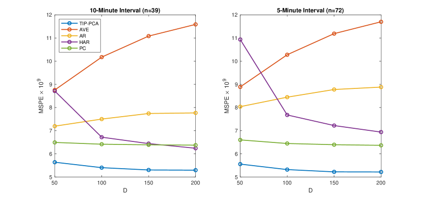
Figure 1: MSPE$\times 10^{9}$ for the TIP-PCA, AVE, AR, HAR, and PC.

Figure 1 presents the average MSPEs of one-day-ahead intraday instantaneous volatility estimators with $D=\{50,100,150,200\}$ and $n=\{39,78\}$. We note that for each simulation, since we used the subsampled data, the target future volatility is the same for each different $D$. Figure 1 makes evident that the TIP-PCA method demonstrates the best performance. This is because TIP-PCA can accurately predict the future instantaneous volatility process by leveraging the features of the HAR model and the U-shaped intraday volatility and handling of the overparameterization problem. Additionally, the MSPEs of TIP-PCA tend to decrease as the number of daily observations and intraday instantaneous volatility estimators increase. This finding aligns with the theoretical results in Section 3. In contrast, the MSPEs of AVE and AR increase as the number of daily observations increases. This may be because they do not include the HAR model feature and consider old information deemed unhelpful. Furthermore, the HAR method does not perform well due to its inability to integrate the U-shaped intraday volatility feature and the overparameterization problem.

5 Empirical Study

In this section, we applied the proposed TIP-PCA method to an intraday instantaneous volatility prediction using real high-frequency trading data. We obtained intraday data of the S&P 500 index ETF (SPY) and ETFs that represent the 11 Global Industrial Classification Standard (GICS) sector index funds (XLC, XLY, XLP, XLE, XLF, XLV, XLI, XLB, XLRE, XLK, and XLU) from July 2021 to June 2022 from the TAQ database in the Wharton Research Data Services (WRDS) system. We used the log prices and employed the jump robust pre-averaging estimation procedure defined in Section 4 to estimate the instantaneous variance at a frequency of every 10 minutes. Then, we conducted the TIP-PCA, AVE, AR, HAR, and PC methods as described in Section 4 using the in-sample period data to predict the one-day-ahead instantaneous volatilities. We used the rolling window scheme, where the in-sample period was 63 days (i.e., one quarter). The number of out-of-sample predictions was 7,371 (i.e., every 10 minutes for 189 days).

Table 1: MSPEs and QLIKEs for the TIP-PCA, AVE, AR, HAR, and PC.

	MSPE$\times 10^{9}$					QLIKE
	TIP-PCA	AVE	AR	HAR	PC	TIP-PCA	AVE	AR	HAR	PC
SPY	2.239	3.213	2.903	3.415	2.407	-9.054	-8.932	-9.095	-9.083	-9.171
XLC	3.308	4.491	4.055	4.917	3.455	-8.871	-8.801	-8.898	-2.205	-8.973
XLY	8.606	11.992	10.327	12.421	9.157	-8.367	-8.179	-8.297	-8.222	-8.379
XLP	0.593	0.798	0.713	0.811	0.604	-9.477	-9.378	-9.444	-9.399	-9.484
XLE	8.471	11.792	9.516	10.150	8.559	-8.090	-8.013	-8.060	-8.544	-8.093
XLF	2.380	3.510	2.854	3.101	2.524	-8.393	-8.327	-8.379	-8.754	-8.391
XLV	0.918	1.223	1.069	1.249	0.953	-9.417	-9.302	-9.391	-9.439	-9.451
XLI	1.817	2.568	2.344	2.894	1.851	-9.134	-8.997	-9.109	-9.132	-9.197
XLB	2.182	2.993	2.605	3.081	2.254	-9.104	-8.947	-9.025	-9.121	-9.118
XLRE	1.803	2.339	2.120	2.422	1.819	-9.082	-8.986	-9.036	-9.002	-9.075
XLK	7.477	10.233	9.019	10.771	7.879	-8.487	-8.316	-8.452	-11.019	-8.511
XLU	0.909	1.143	1.026	1.127	0.926	-9.122	-9.057	-9.097	-9.037	-9.117

To measure the performance of the predicted instantaneous volatility, we utilized the mean squared prediction errors (MSPE) and QLIKE (Patton, 2011) as follows:

$$\text{MSPE}=\frac{1}{nq}\sum_{i=1}^{q}\sum_{j=1}^{n}(\widetilde{c}_{D+i,j}-\widehat{c}_{D+i,j})^{2},$$

$$\text{QLIKE}=\frac{1}{nq}\sum_{i=1}^{q}\sum_{j=1}^{n}(\log{\widetilde{c}_{D+i,j}}+\frac{\widehat{c}_{D+i,j}}{\widetilde{c}_{D+i,j}}),$$

where $\widetilde{c}_{D+i,j}$ is one of the TIP-PCA, AVE, AR, HAR, and PC estimates. We predicted one-day-ahead conditional expected instantaneous volatilities using in-sample period data. Additionally, since we do not know the true conditional expected instantaneous volatility, to assess the significance of differences in prediction performances, we conducted the Diebold and Mariano (DM) test (Diebold and Mariano, 2002) based on MSPE and QLIKE. We compared the proposed TIP-PCA method with other methods. Table 1 reports the results of MSPEs and QLIKEs, and Table 2 shows the $p$-values for the DM tests. From Tables 1 and 2, we find that the TIP-PCA method exhibits the best performance overall. This may be because the projection method, utilizing covariates such as ex-post realized volatility information and the U-shaped intraday volatility feature, contributes to enhancing the accuracy of instantaneous volatility predictions.

Table 2: The p-values for the DM test statistic based on MSPE and QLIKE for AVE, AR, HAR, and PC with respect to the TIP-PCA.

	MSPE				QLIKE
	AVE	AR	HAR	PC	AVE	AR	HAR	PC
SPY	0.000∗∗∗	0.000∗∗∗	0.000∗∗∗	0.000∗∗∗	0.000∗∗∗	0.043∗∗	0.620	0.000∗∗∗
XLC	0.000∗∗∗	0.000∗∗∗	0.000∗∗∗	0.005∗∗∗	0.019∗∗	0.284	0.331	0.000∗∗∗
XLY	0.000∗∗∗	0.000∗∗∗	0.000∗∗∗	0.000∗∗∗	0.000∗∗∗	0.000∗∗∗	0.067∗	0.000∗∗∗
XLP	0.000∗∗∗	0.000∗∗∗	0.000∗∗∗	0.391	0.000∗∗∗	0.000∗∗∗	0.165	0.000∗∗∗
XLE	0.000∗∗∗	0.000∗∗∗	0.000∗∗∗	0.789	0.000∗∗∗	0.000∗∗∗	0.211	0.107
XLF	0.000∗∗∗	0.000∗∗∗	0.000∗∗∗	0.000∗∗∗	0.000∗∗∗	0.000∗∗∗	0.366	0.017∗∗
XLV	0.000∗∗∗	0.000∗∗∗	0.000∗∗∗	0.082∗	0.000∗∗∗	0.001∗∗∗	0.529	0.000∗∗∗
XLI	0.000∗∗∗	0.000∗∗∗	0.000∗∗∗	0.081∗	0.000∗∗∗	0.021∗∗	0.818	0.000∗∗∗
XLB	0.000∗∗∗	0.000∗∗∗	0.000∗∗∗	0.019∗∗	0.000∗∗∗	0.000∗∗∗	0.799	0.000∗∗∗
XLRE	0.000∗∗∗	0.000∗∗∗	0.000∗∗∗	0.517	0.000∗∗∗	0.000∗∗∗	0.397	0.050∗
XLK	0.000∗∗∗	0.000∗∗∗	0.000∗∗∗	0.000∗∗∗	0.000∗∗∗	0.000∗∗∗	0.333	0.000∗∗∗
XLU	0.000∗∗∗	0.001∗∗∗	0.000∗∗∗	0.168	0.000∗∗∗	0.000∗∗∗	0.000∗∗∗	0.002∗∗∗

• Note: ***, **, and * indicate that the proposed TIP-PCA method outperforms the corresponding method with 1%, 5%, and 10% significance levels, respectively.

We also evaluated the performance of the proposed method in estimating one-day-ahead 10-minute frequency Value at Risk (VaR). In particular, we first predicted the one-day-ahead conditional expected instantaneous volatilities using the TIP-PCA, AVE, AR, HAR, and PC procedures using the in-sample period data. We then calculated the quantiles using historical standardized 10-minute returns. Specifically, we standardized in-sample 10-minute returns using estimated conditional instantaneous volatilities. We then derived sample quantiles for 0.01, 0.02, 0.05, 0.1, and 0.2. Using the sample quantile estimates and predicted instantaneous volatility, we obtained the one-day-ahead 10-minute frequency VaR values for each prediction method. We used a fixed in-sample period as one quarter and implemented a rolling window scheme. The out-of-sample period was considered to be from October 2021 to June 2022.

To backtest the estimated VaR, we conducted the likelihood ratio unconditional coverage (LRuc) test (Kupiec, 1995), the likelihood ratio conditional coverage (LRcc) test (Christoffersen, 1998), and the dynamic quantile (DQ) test with lag 4 (Engle and Manganelli, 2004). Table 3 reports the number of cases where the $p$-value is greater than 0.05 for the 12 ETFs at each $q_{0}=\{0.01,0.02,0.05,0.1,0.2\}$ quantile, based on the LRuc, LRcc, and DQ tests. From Table 3, we find that the TIP-PCA method consistently outperforms in all hypothesis tests. This outcome confirms that the proposed TIP-PCA method, incorporating crucial market intraday and interday dynamic information, significantly contributes to the improved prediction accuracy of future instantaneous volatilities and enhanced risk management.

Table 3: Number of cases where the $p$-value is greater than 0.05 for TIP-PCA, AVE, AR, HAR, and PC across 12 ETFs at each $q_{0}=\{0.01,0.02,0.05,0.1,0.2\}$ based on the LRuc, LRcc, and DQ tests.

	LRuc					LRcc					DQ
$q_{0}$	0.01	0.02	0.05	0.1	0.2	0.01	0.02	0.05	0.1	0.2	0.01	0.02	0.05	0.1	0.2
TIP-PCA	7	9	12	12	12	9	8	11	12	12	5	5	7	7	9
AVE	2	2	1	12	12	2	3	2	11	12	3	3	4	4	7
AR	3	3	8	12	12	5	5	10	12	12	3	4	5	7	8
HAR	0	1	3	12	12	0	1	2	7	12	2	3	3	4	6
PC	6	6	11	12	12	4	6	11	11	12	4	4	6	7	9

6 Conclusion

This paper introduces a novel intraday instantaneous volatility prediction procedure. The proposed Two-sIde-Projected-PCA (TIP-PCA) method leverages both interday and intraday volatility dynamics based on the semiparametric structure of the low-rank matrix of the instantaneous volatility process. We establish the asymptotic properties of TIP-PCA and its future instantaneous volatility estimators. In the empirical study, concerning the out-of-sample performance of predicting the one-day-ahead instantaneous volatility process, TIP-PCA outperforms other conventional methods. This finding confirms that both the HAR model structure on interday dynamics and the U-shaped pattern on intraday dynamics contribute to predicting the future instantaneous volatility process.

In this paper, we focus on the instantaneous volatility process for a single asset. In practice, we often need to handle a large number of assets. Thus, it is important and interesting to extend the study to predicting the instantaneous volatility process of many assets. However, to do this, cross-sectionally, we encounter another curse of dimensionality. Therefore, technically, it is a demanding task to handle both the cross-sectional curse of dimensionality and the intraday curse of dimensionality. We leave this for a future study.

Appendix A Proofs

A.1 Related Lemmas

Lemma A.1.

Under Assumptions 3.1 and 3.4, for $k\leq r$, we have

$$|\widehat{\lambda}_{k}-\lambda_{k}| =O_{P}\left(m^{-\frac{1}{8}}\sqrt{nD\log(nD)}+\sqrt{D\log D}+\sqrt{\frac{n}{D}}\varphi_{D}\right).$$

Proof.

Let $\widehat{\bm{\Lambda}}=\mathrm{diag}(\widehat{\lambda}_{1},\dots,\widehat{\lambda}_{r}),$ where $\widehat{\lambda}_{1}\geq\widehat{\lambda}_{2}\geq\cdots\geq\widehat{\lambda}_{r}$ are the square root of leading eigenvalues of $\widehat{\bm{\Sigma}}_{D,n}\widehat{\bm{\Sigma}}_{D,n}^{\prime}$. Let $\bm{\Omega}_{D\times D}$ be the $D\times D$ covariance matrix of $\mathbf{c}_{j}=(c_{1,j},\ldots,c_{D,j})^{\prime}$ such that $\bm{\Omega}_{D\times D}=\frac{1}{n}\mathbf{U}\bm{\Lambda}^{2}\mathbf{U}^{\prime}+\bm{\Omega}_{\varepsilon,D\times D}$, where $\bm{\Omega}_{\varepsilon,D\times D}$ is the $D\times D$ covariance matrix of $\mbox{\boldmath$\varepsilon$}_{j}=(\varepsilon_{1,j},\ldots,\varepsilon_{D,j})^{\prime}$. By Weyl’s theorem, we have

$$\|\widehat{\bm{\Lambda}}^{2}-\bm{\Lambda}^{2}\|_{\max} \leq\|\widehat{\bm{\Sigma}}_{D,n}\widehat{\bm{\Sigma}}_{D,n}^{\prime}-\mathbf{U}\bm{\Lambda}^{2}\mathbf{U}^{\prime}\|$$

$$\leq\|\widehat{\bm{\Sigma}}_{D,n}\widehat{\bm{\Sigma}}_{D,n}^{\prime}-\bm{\Sigma}_{D,n}\bm{\Sigma}_{D,n}^{\prime}\|+\|\bm{\Sigma}_{D,n}\bm{\Sigma}_{D,n}^{\prime}-\mathbf{U}\bm{\Lambda}^{2}\mathbf{U}^{\prime}\|$$

$$\leq\|\widehat{\bm{\Sigma}}_{D,n}\widehat{\bm{\Sigma}}_{D,n}^{\prime}-\bm{\Sigma}_{D,n}\bm{\Sigma}_{D,n}^{\prime}\|_{F}+\|\bm{\Sigma}_{D,n}\bm{\Sigma}_{D,n}^{\prime}-n\bm{\Omega}_{D\times D}\|+\|n\bm{\Omega}_{D\times D}-\mathbf{U}\bm{\Lambda}^{2}\mathbf{U}^{\prime}\|$$

$$=O_{P}(nDm^{-\frac{1}{8}}\sqrt{\log(nD)}+D\sqrt{n\log D}+n\varphi_{D}),$$

where the last line is due to Assumptions 3.1 and 3.4. Therefore, for $k\leq r$, we have

$$|\widehat{\lambda}_{k}-\lambda_{k}|\leq\frac{|\widehat{\lambda}_{k}^{2}-\lambda_{k}^{2}|}{\widehat{\lambda}_{k}+\lambda_{k}}=O_{P}\left(m^{-\frac{1}{8}}\sqrt{nD\log(nD)}+\sqrt{D\log D}+\sqrt{\frac{n}{D}}\varphi_{D}\right).$$

∎

Let $\widetilde{\mathbf{G}}(\mathbf{X})$ and $\widetilde{\mathbf{H}}(\mathbf{W})$ be the singular vector estimators that the signs are matched such that $\widetilde{\mathbf{G}}(\mathbf{X})\widehat{\bm{\Lambda}}\widetilde{\mathbf{H}}(\mathbf{W})=\sum_{k=1}^{r}s_{0k}\widehat{\lambda}_{k}\widehat{U}_{k}\widehat{V}_{k}^{\prime},$ where $s_{0k}=\mbox{sign}(\langle\widehat{U}_{k},U_{k}\rangle)\mbox{sign}(\langle\widehat{V}_{k},V_{k}\rangle)$ for $k=1,\dots,r$. The following lemma presents the individual convergence rate of singular vector estimators given the true sign.

Lemma A.2.

Under Assumptions 3.1–3.4, we have the following results:

(i) $$\|\widetilde{\mathbf{G}}(\mathbf{X})-\mathbf{G}(\mathbf{X})\|_{\max}=O_{P}\left(\frac{J_{1}m^{-\frac{1}{8}}\sqrt{\log(nD)}}{\sqrt{D}}+\frac{J_{1}^{\frac{1}{2}-\frac{\kappa}{2}}}{\sqrt{D}}+\frac{J_{1}}{D}\right),$$

(ii) $$\|\widetilde{\mathbf{H}}(\mathbf{W})-\mathbf{H}(\mathbf{W})\|_{\max}=O_{P}\left(\frac{J_{2}m^{-\frac{1}{8}}\sqrt{\log(nD)}}{\sqrt{n}}+\frac{J_{2}^{\frac{1}{2}-\frac{\kappa}{2}}}{\sqrt{n}}+\frac{J_{2}}{n}\right).$$

Proof.

We first consider $(i)$. Let $\widetilde{\mathbf{G}}(\mathbf{X})=(\widehat{U}_{1},\ldots,\widehat{U}_{r})$ and $\mathbf{G}(\mathbf{X})=(U_{1},\ldots,U_{r})$. We denote the eigengap $\bar{\gamma}=\min\{\lambda_{k}^{2}-\lambda_{k+1}^{2}:1\leq k\leq r\}$ and $\lambda_{r+1}=0$. For $k\leq r$, $\lambda_{k}\asymp\sqrt{nD}$ and $\|U_{k}\|_{\infty}\leq C/\sqrt{D}$. In addition, the coherence $\mu(\mathbf{U})=D\max_{i}\sum_{k=1}^{r}u_{i,k}^{2}/r\leq C$, where $u_{i,k}$ is the $(i,k)$ entry of $\mathbf{U}$. Thus, by Theorem 1 of Fan et al. (2018b), we have

$$\max_{k\leq r}\|\widehat{U}_{k}-U_{k}\|_{\infty}$$

$$\leq C\frac{\|\mathbf{P}_{\Phi}\widehat{\bm{\Sigma}}_{D,n}\widehat{\bm{\Sigma}}_{D,n}^{\prime}\mathbf{P}_{\Phi}-\mathbf{U}\bm{\Lambda}^{2}\mathbf{U}^{\prime}\|_{\infty}}{\bar{\gamma}\sqrt{D}}$$

$$\leq C\frac{\|\mathbf{P}_{\Phi}\widehat{\bm{\Sigma}}_{D,n}\widehat{\bm{\Sigma}}_{D,n}^{\prime}\mathbf{P}_{\Phi}-\mathbf{P}_{\Phi}\bm{\Sigma}_{D,n}\bm{\Sigma}_{D,n}^{\prime}\mathbf{P}_{\Phi}\|_{\infty}+\|\mathbf{P}_{\Phi}\bm{\Sigma}_{D,n}\bm{\Sigma}_{D,n}^{\prime}\mathbf{P}_{\Phi}-\mathbf{U}\bm{\Lambda}^{2}\mathbf{U}^{\prime}\|_{\infty}}{\bar{\gamma}\sqrt{D}}$$

$$=O_{P}\left(\frac{J_{1}m^{-\frac{1}{8}}\sqrt{\log(nD)}}{\sqrt{D}}+\frac{J_{1}^{\frac{1}{2}-\frac{\kappa}{2}}}{\sqrt{D}}+\frac{J_{1}}{D}\right),$$

where the last line is due to Lemma A.3 below. By using the similar argument, we can obtain the result (ii).

∎

Lemma A.3.

Under Assumptions 3.1–3.4, we have

• $\|\mathbf{P}_{\Phi}\widehat{\bm{\Sigma}}_{D,n}\widehat{\bm{\Sigma}}_{D,n}^{\prime}\mathbf{P}_{\Phi}-\mathbf{P}_{\Phi}\bm{\Sigma}_{D,n}\bm{\Sigma}_{D,n}^{\prime}\mathbf{P}_{\Phi}\|_{\max}=O_{P}(J_{1}nm^{-\frac{1}{8}}\sqrt{\log(nD)})$,

• $\|\mathbf{P}_{\Phi}\bm{\Sigma}_{D,n}\bm{\Sigma}_{D,n}^{\prime}\mathbf{P}_{\Phi}-\mathbf{U}\bm{\Lambda}^{2}\mathbf{U}^{\prime}\|_{\max}=O_{P}(nJ_{1}^{1/2-\kappa/2}+nJ_{1}/\sqrt{D})$.

Proof.

We first consider $(i)$. By Assumptions 3.1 and 3.2, $\|\widehat{\bm{\Sigma}}_{D,n}\widehat{\bm{\Sigma}}_{D,n}^{\prime}-\bm{\Sigma}_{D,n}\bm{\Sigma}_{D,n}^{\prime}\|_{F}=O_{P}(nDm^{-\frac{1}{8}}\sqrt{\log(nd)})$, $\|(\bm{\Phi}(\mathbf{X})^{\prime}\bm{\Phi}(\mathbf{X}))^{-1}\|=\lambda_{\min}^{-1}(D^{-1}\bm{\Phi}(\mathbf{X})^{\prime}\bm{\Phi}(\mathbf{X}))D^{-1}=O_{P}(D^{-1})$, and $\|\bm{\Phi}(\mathbf{X})\|=O_{P}(D^{1/2})$. Then, we can show

$$\|\mathbf{P}_{\Phi}\widehat{\bm{\Sigma}}_{D,n}\widehat{\bm{\Sigma}}_{D,n}^{\prime}\mathbf{P}_{\Phi}-\mathbf{P}_{\Phi}\bm{\Sigma}_{D,n}\bm{\Sigma}_{D,n}^{\prime}\mathbf{P}_{\Phi}\|_{\max}$$

$$\quad=\max_{i,j}|\phi(\mathbf{x}_{i})(\bm{\Phi}(\mathbf{X})^{\prime}\bm{\Phi}(\mathbf{X}))^{-1}\bm{\Phi}(\mathbf{X})^{\prime}(\widehat{\bm{\Sigma}}_{D,n}\widehat{\bm{\Sigma}}_{D,n}^{\prime}-\bm{\Sigma}_{D,n}\bm{\Sigma}_{D,n}^{\prime})\bm{\Phi}(\mathbf{X})(\bm{\Phi}(\mathbf{X})^{\prime}\bm{\Phi}(\mathbf{X}))^{-1}\phi(\mathbf{x}_{j})^{\prime})$$

$$\quad\leq\max_{i}\|\phi(\mathbf{x}_{i})\|_{F}^{2}\|(\bm{\Phi}(\mathbf{X})^{\prime}\bm{\Phi}(\mathbf{X}))^{-1}\|^{2}\|\bm{\Phi}(\mathbf{X})^{\prime}\|^{2}\|\widehat{\bm{\Sigma}}_{D,n}\widehat{\bm{\Sigma}}_{D,n}^{\prime}-\bm{\Sigma}_{D,n}\bm{\Sigma}_{D,n}^{\prime}\|_{F}$$

$$\quad=O_{P}(J_{1}nm^{-\frac{1}{8}}\sqrt{\log(nD)}).$$

We consider $(ii)$. Note that $\mathbf{P}_{\Phi}\bm{\Sigma}_{D,n}=\bm{\Phi}(\mathbf{X})\mathbf{B}\bm{\Lambda}\mathbf{V}^{\prime}+\mathbf{P}_{\Phi}\mathbf{R}(\mathbf{X})\bm{\Lambda}\mathbf{V}^{\prime}+\mathbf{P}_{\Phi}\bm{\Sigma}_{\varepsilon}$. We have

$$\|\mathbf{P}_{\Phi}\bm{\Sigma}_{D,n}\bm{\Sigma}_{D,n}^{\prime}\mathbf{P}_{\Phi}-\mathbf{U}\bm{\Lambda}^{2}\mathbf{U}^{\prime}\|_{\max}$$

$$\leq\|\mathbf{P}_{\Phi}\bm{\Sigma}_{D,n}\bm{\Sigma}_{D,n}^{\prime}\mathbf{P}_{\Phi}-\bm{\Phi}(\mathbf{X})\mathbf{B}\bm{\Lambda}^{2}\mathbf{B}^{\prime}\bm{\Phi}(\mathbf{X})^{\prime}\|_{\max}+\|\bm{\Phi}(\mathbf{X})\mathbf{B}\bm{\Lambda}^{2}\mathbf{B}^{\prime}\bm{\Phi}(\mathbf{X})^{\prime}-\mathbf{U}\bm{\Lambda}^{2}\mathbf{U}^{\prime}\|_{\max}$$

$$=\|\bm{\Phi}(\mathbf{X})\mathbf{B}\bm{\Lambda}^{2}\mathbf{R}(\mathbf{X})^{\prime}\mathbf{P}_{\Phi}+\bm{\Phi}(\mathbf{X})\mathbf{B}\bm{\Lambda}\mathbf{V}^{\prime}\bm{\Sigma}_{\varepsilon}^{\prime}\mathbf{P}_{\Phi}+\mathbf{P}_{\Phi}\mathbf{R}(\mathbf{X})\bm{\Lambda}^{2}\mathbf{R}(\mathbf{X})^{\prime}\mathbf{P}_{\Phi}$$

$$\qquad+\mathbf{P}_{\Phi}\mathbf{R}(\mathbf{X})\bm{\Lambda}\mathbf{V}^{\prime}\bm{\Sigma}_{\varepsilon}^{\prime}\mathbf{P}_{\Phi}+\mathbf{P}_{\Phi}\bm{\Sigma}_{\varepsilon}\bm{\Sigma}_{\varepsilon}^{\prime}\mathbf{P}_{\Phi}\|_{\max}+\|\bm{\Phi}(\mathbf{X})\mathbf{B}\bm{\Lambda}^{2}\mathbf{R}(\mathbf{X})^{\prime}+\mathbf{R}(\mathbf{X})\bm{\Lambda}^{2}\mathbf{R}(\mathbf{X})^{\prime}\|_{\max}.$$

$$=O_{P}(nJ_{1}^{1/2-\kappa/2}+nJ_{1}/\sqrt{D}),$$

where the last line is due to the results in Lemma A.4 below. ∎

Lemma A.4.

Under Assumptions 3.2–3.4, we have the following rates:

• $\|\bm{\Phi}(\mathbf{X})\mathbf{B}\bm{\Lambda}^{2}\mathbf{R}(\mathbf{X})^{\prime}\mathbf{P}_{\Phi}\|_{\max}=O_{P}(nJ_{1}^{(1-\kappa)/2})$, $\|\bm{\Phi}(\mathbf{X})\mathbf{B}\bm{\Lambda}^{2}\mathbf{R}(\mathbf{X})^{\prime}\|_{\max}=O_{P}(nJ_{1}^{-\kappa/2})$.

• $\|\bm{\Phi}(\mathbf{X})\mathbf{B}\bm{\Lambda}\mathbf{V}^{\prime}\bm{\Sigma}_{\varepsilon}^{\prime}\mathbf{P}_{\Phi}\|_{\max}=O_{P}(nJ_{1}/\sqrt{D})$.

• $\|\mathbf{P}_{\Phi}\mathbf{R}(\mathbf{X})\bm{\Lambda}^{2}\mathbf{R}(\mathbf{X})^{\prime}\mathbf{P}_{\Phi}\|_{\max}=O_{P}(nJ_{1}^{1-\kappa})$, $\|\mathbf{R}(\mathbf{X})\bm{\Lambda}^{2}\mathbf{R}(\mathbf{X})^{\prime}\|_{\max}=O_{P}(nJ_{1}^{-\kappa})$.

• $\|\mathbf{P}_{\Phi}\mathbf{R}(\mathbf{X})\bm{\Lambda}\mathbf{V}^{\prime}\bm{\Sigma}_{\varepsilon}^{\prime}\mathbf{P}_{\Phi}\|_{\max}=O_{P}(nJ_{1}^{(3-\kappa)/2}/\sqrt{D})$, $\|\mathbf{P}_{\Phi}\bm{\Sigma}_{\varepsilon}\bm{\Sigma}_{\varepsilon}^{\prime}\mathbf{P}_{\Phi}\|_{\max}=O_{P}(nJ_{1}^{2}/D)$.

Proof.

(i) Let $\phi(\mathbf{x}_{i})$ and $R(\mathbf{x}_{i})$ be the $i$th row of $\bm{\Phi}(\mathbf{X})$ and $\mathbf{R}(\mathbf{X})$, respectively. By Assumptions 3.2 and 3.3, we have $\|\phi(\mathbf{x}_{i})\mathbf{B}\|_{F}=O_{P}(1/\sqrt{D})$ and $\|R(\mathbf{x}_{i})\|_{F}=O_{P}(J_{1}^{-\kappa/2}/\sqrt{D})$, for each $i\leq D$. Also, by Assumption 3.3 (ii), we have $\|\mathbf{R}(\mathbf{X})\|_{F}=O_{P}(J_{1}^{-\kappa/2})$, and by Assumption 3.2 (i), $\|(\bm{\Phi}(\mathbf{X})^{\prime}\bm{\Phi}(\mathbf{X}))^{-1}\|=O_{P}(D^{-1})$ and $\|\bm{\Phi}(\mathbf{X})\|=O_{P}(D^{1/2})$. Then, we can obtain

$$\max_{i,j\leq D}|\phi(\mathbf{x}_{i})\mathbf{B}\bm{\Lambda}^{2}\mathbf{R}(\mathbf{X})\bm{\Phi}(\mathbf{X})(\bm{\Phi}(\mathbf{X})^{\prime}\bm{\Phi}(\mathbf{X}))^{-1}\phi(\mathbf{x}_{j})^{\prime}|$$

$$\leq\max_{i}\|\phi(\mathbf{x}_{i})\mathbf{B}\|_{F}\|\bm{\Lambda}^{2}\|\|\mathbf{R}(\mathbf{X})\|_{F}\|\bm{\Phi}(\mathbf{X})\|\|(\bm{\Phi}(\mathbf{X})^{\prime}\bm{\Phi}(\mathbf{X}))^{-1}\|\max_{i}\|\phi(\mathbf{x}_{i})^{\prime}\|_{F}$$

$$=O_{P}(nJ_{1}^{1/2-\kappa/2}),$$

and

$$\max_{i,j\leq D}|\phi(\mathbf{x}_{i})\mathbf{B}\bm{\Lambda}^{2}R(\mathbf{x}_{j})|\leq\max_{i}\|\phi(\mathbf{x}_{i})\mathbf{B}\|_{F}\|\bm{\Lambda}^{2}\|\max_{i}\|R(\mathbf{x}_{i})\|_{F}=O_{P}(nJ_{1}^{-\kappa/2}).$$

(ii) By Lemma A.5 (ii), we have

$$\max_{i,j\leq D}|\phi(\mathbf{x}_{i})\mathbf{B}\bm{\Lambda}\mathbf{V}^{\prime}\bm{\Sigma}_{\varepsilon}^{\prime}\bm{\Phi}(\mathbf{X})(\bm{\Phi}(\mathbf{X})^{\prime}\bm{\Phi}(\mathbf{X}))^{-1}\phi(\mathbf{x}_{j})^{\prime}|$$

$$\leq\max_{i}\|\phi(\mathbf{x}_{i})\mathbf{B}\|_{F}\|\bm{\Lambda}\|\|\mathbf{V}^{\prime}\bm{\Sigma}_{\varepsilon}^{\prime}\bm{\Phi}(\mathbf{X})\|_{F}\|(\bm{\Phi}(\mathbf{X})^{\prime}\bm{\Phi}(\mathbf{X}))^{-1}\|\max_{i}\|\phi(\mathbf{x}_{i})^{\prime}\|_{F}$$

$$=O_{P}(nJ_{1}/\sqrt{D}).$$

(iii) We have

$$\max_{i,j\leq D}|\phi(\mathbf{x}_{i})(\bm{\Phi}(\mathbf{X})^{\prime}\bm{\Phi}(\mathbf{X}))^{-1}\bm{\Phi}(\mathbf{X})^{\prime}\mathbf{R}(\mathbf{X})\bm{\Lambda}^{2}\mathbf{R}(\mathbf{X})^{\prime}\bm{\Phi}(\mathbf{X})(\bm{\Phi}(\mathbf{X})^{\prime}\bm{\Phi}(\mathbf{X}))^{-1}\phi(\mathbf{x}_{j})^{\prime}|$$

$$\qquad\leq\max_{i}\|\phi(\mathbf{x}_{i})\|_{F}^{2}\|(\bm{\Phi}(\mathbf{X})^{\prime}\bm{\Phi}(\mathbf{X}))^{-1}\|^{2}\|\bm{\Phi}(\mathbf{X})\|^{2}\|\mathbf{R}(\mathbf{X})\|_{F}^{2}\|\bm{\Lambda}^{2}\|$$

$$\qquad=O_{P}(nJ_{1}^{1-\kappa}),$$

and

$$\max_{i,j\leq D}|R(\mathbf{x}_{i})\bm{\Lambda}^{2}R(\mathbf{x}_{j})^{\prime}|\leq\max_{i}\|R(\mathbf{x}_{i})\|_{F}^{2}\|\bm{\Lambda}^{2}\|=O_{P}(nJ_{1}^{-\kappa}).$$

(iv) By Lemma A.5, we have

$$\max_{i,j\leq D}|\phi(\mathbf{x}_{i})(\bm{\Phi}(\mathbf{X})^{\prime}\bm{\Phi}(\mathbf{X}))^{-1}\bm{\Phi}(\mathbf{X})^{\prime}\mathbf{R}(\mathbf{X})\bm{\Lambda}\mathbf{V}^{\prime}\bm{\Sigma}_{\varepsilon}^{\prime}\bm{\Phi}(\mathbf{X})(\bm{\Phi}(\mathbf{X})^{\prime}\bm{\Phi}(\mathbf{X}))^{-1}\phi(\mathbf{x}_{j})^{\prime}|$$

$$\quad\leq\max_{i}\|\phi(\mathbf{x}_{i})\|_{F}^{2}\|(\bm{\Phi}(\mathbf{X})^{\prime}\bm{\Phi}(\mathbf{X}))^{-1}\|^{2}\|\bm{\Phi}(\mathbf{X})^{\prime}\|\|\mathbf{R}(\mathbf{X})\|_{F}\|\bm{\Lambda}\|\|\mathbf{V}^{\prime}\bm{\Sigma}_{\varepsilon}^{\prime}\bm{\Phi}(\mathbf{X})\|_{F}$$

$$\quad=O_{P}(nJ_{1}^{(3-\kappa)/2}/\sqrt{D}),$$

and

$$\max_{i,j\leq D}|\phi(\mathbf{x}_{i})(\bm{\Phi}(\mathbf{X})^{\prime}\bm{\Phi}(\mathbf{X}))^{-1}\bm{\Phi}(\mathbf{X})^{\prime}\bm{\Sigma}_{\varepsilon}\bm{\Sigma}_{\varepsilon}^{\prime}\bm{\Phi}(\mathbf{X})(\bm{\Phi}(\mathbf{X})^{\prime}\bm{\Phi}(\mathbf{X}))^{-1}\phi(\mathbf{x}_{j})^{\prime}|$$

$$\qquad\leq\max_{i}\|\phi(\mathbf{x}_{i})\|_{F}^{2}\|(\bm{\Phi}(\mathbf{X})^{\prime}\bm{\Phi}(\mathbf{X}))^{-1}\|^{2}\|\bm{\Phi}(\mathbf{X})^{\prime}\bm{\Sigma}_{\varepsilon}\|_{F}^{2}=O_{P}(nJ_{1}^{2}/D).$$

∎

Lemma A.5.

Under Assumptions 3.2–3.4, we have the following rates:

• $\max_{i\leq D}\max_{j\leq n}\sum_{s=1}^{n}|E\varepsilon_{i,j}\varepsilon_{i,s}|=O(1)$,
  $\max_{k\leq r,i\leq D}\max_{j\leq n}\sum_{s=1}^{n}|\mathrm{cov}(v_{j,k}\varepsilon_{i,t},v_{s,k}\varepsilon_{i,s})|=O(1)$,
  $\max_{i\leq D,m\leq D}\max_{j\leq n}\sum_{s=1}^{n}|\mathrm{cov}(\varepsilon_{i,j}\varepsilon_{m,s},\varepsilon_{i,s}\varepsilon_{m,s})|=O(1)$.

• $\|\bm{\Phi}(\mathbf{X})^{\prime}\bm{\Sigma}_{\varepsilon}\|_{F}=O_{P}(\sqrt{nDJ_{1}})$, $\|\bm{\Phi}(\mathbf{X})^{\prime}\bm{\Sigma}_{\varepsilon}\mathbf{V}\|_{F}=O_{P}(\sqrt{nDJ_{1}}).$

Proof.

(i) The results follow from Davydov’s inequality, which are similar to Lemma B.1 in the supplementary material of Fan et al. (2016b).
(ii) By the Cauchy Schwarz inequality, part (i), and Assumption 3.4, we can obtain

$$E\|\bm{\Sigma}_{\varepsilon}^{\prime}\bm{\Phi}(\mathbf{X})\|_{F}^{2} =\sum_{j=1}^{n}\sum_{l=1}^{J_{1}}\sum_{d=1}^{d_{1}}E(\sum_{i=1}^{D}\phi_{l}(x_{id})\varepsilon_{i,j})^{2}$$

$$=\sum_{j=1}^{n}\sum_{jl1}^{J_{1}}\sum_{d=1}^{d_{1}}\sum_{i=1}^{D}\sum_{m=1}^{D}E\phi_{l}(x_{id})\phi_{l}(x_{md})E\varepsilon_{i,j}\varepsilon_{m,j}$$

$$\leq J_{1}d_{1}D\max_{l\leq J_{1},d\leq d_{1},i\leq D}E\phi_{l}(x_{id})^{2}\sum_{j=1}^{n}\max_{m\leq D}\sum_{i=1}^{D}|E\varepsilon_{i,j}\varepsilon_{m,j}|=O(nDJ_{1}),$$

and

$$E\|\bm{\Phi}(\mathbf{X})^{\prime}\bm{\Sigma}_{\varepsilon}\mathbf{V}\|_{F}^{2}=\sum_{k=1}^{r}\sum_{l=1}^{J_{1}}\sum_{d=1}^{d_{1}}E(\sum_{i=1}^{D}\sum_{j=1}^{n}\phi_{l}(x_{id})\varepsilon_{i,j}v_{j,k})^{2}$$

$$=\sum_{k=1}^{r}\sum_{l=1}^{J_{1}}\sum_{d=1}^{d_{1}}\mbox{var}(\sum_{i=1}^{D}\sum_{j=1}^{n}\phi_{l}(x_{id})\varepsilon_{i,j}v_{j,k})$$

$$=\sum_{k=1}^{r}\sum_{l=1}^{J_{1}}\sum_{d=1}^{d_{1}}\sum_{i=1}^{D}\sum_{j=1}^{n}\mbox{var}(\phi_{l}(x_{id})\varepsilon_{i,j}v_{j,k})+\sum_{k,l,d,i}\sum_{j\neq s;j,s\leq n}(E\phi_{l}(x_{id})^{2}v_{j,k}v_{s,k})E\varepsilon_{i,j}\varepsilon_{i,s}$$

$$\;\;\;+\sum_{k=1}^{r}\sum_{l=1}^{J_{1}}\sum_{d=1}^{d_{1}}\sum_{i\neq m;i,m\leq D}\sum_{j,s\leq n}(E\phi_{l}(x_{id})\phi_{l}(x_{md})v_{j,k}v_{s,k})E\varepsilon_{i,j}\varepsilon_{m,s}$$

$$\leq O(nDJ_{1})+O(nDJ_{1})\max_{i\leq D,j\leq n}\sum_{s=1}^{n}|E\varepsilon_{i,j}\varepsilon_{i,s}|+O(nDJ_{1})\frac{1}{nD}\sum_{i,m\leq D}\sum_{j,s\leq n}|E\varepsilon_{i,j}\varepsilon_{m,s}|$$

$$=O(nDJ_{1}).$$

∎

A.2 Proof of Proposition 3.1

Proof of Proposition 3.1. We recall that $\widetilde{\mathbf{G}}(\mathbf{X})\widehat{\bm{\Lambda}}\widetilde{\mathbf{H}}(\mathbf{W})=\sum_{k=1}^{r}s_{0k}\widehat{\lambda}_{k}\widehat{U}_{k}\widehat{V}_{k}^{\prime},$ where $s_{0k}$ is the true sign for $k=1,\dots,r$. By Lemmas A.1–A.2, we have

$$\|\widetilde{\mathbf{G}}(\mathbf{X})\widehat{\bm{\Lambda}}\widetilde{\mathbf{H}}(\mathbf{W})^{\prime}-\mathbf{G}(\mathbf{X})\bm{\Lambda}\mathbf{H}(\mathbf{W})^{\prime}\|_{\max}$$

$$\qquad\leq\|\widetilde{\mathbf{G}}(\mathbf{X})(\widehat{\bm{\Lambda}}-\bm{\Lambda})\widetilde{\mathbf{H}}(\mathbf{W})^{\prime}\|_{\max}+\|(\widetilde{\mathbf{G}}(\mathbf{X})-\mathbf{G}(\mathbf{X}))\bm{\Lambda}(\widetilde{\mathbf{H}}(\mathbf{W})-\mathbf{H}(\mathbf{W}))^{\prime}\|_{\max}$$

$$\qquad\qquad+\|\mathbf{G}(\mathbf{X})\bm{\Lambda}(\widetilde{\mathbf{H}}(\mathbf{W})-\mathbf{H}(\mathbf{W}))^{\prime}\|_{\max}+\|(\widetilde{\mathbf{G}}(\mathbf{X})-\mathbf{G}(\mathbf{X}))\bm{\Lambda}\mathbf{H}(\mathbf{W})^{\prime}\|_{\max}$$

$$\qquad=O_{P}\left(\frac{1}{\sqrt{nD}}\|\widehat{\bm{\Lambda}}-\bm{\Lambda}\|_{\max}+\sqrt{D}\|\widetilde{\mathbf{G}}(\mathbf{X})-\mathbf{G}(\mathbf{X})\|_{\max}+\sqrt{n}\|\widetilde{\mathbf{H}}(\mathbf{W})-\mathbf{H}(\mathbf{W})\|_{\max}\right)$$

$$\qquad=O_{P}\left(\max(J_{1},J_{2})m^{-\frac{1}{8}}\sqrt{\log(nD)}+\sqrt{\frac{\log D}{n}}+\frac{\varphi_{D}}{D}+J_{1}^{\frac{1}{2}-\frac{\kappa}{2}}+\frac{J_{1}}{\sqrt{D}}+J_{2}^{\frac{1}{2}-\frac{\kappa}{2}}+\frac{J_{2}}{\sqrt{n}}\right).$$

Then, for any given $\eta>0$, we can find $C_{\eta}>0$ such that for large $m$, $n$ and $D$,

$$\mathbb{P}\left(\frac{1}{\alpha_{m,n,D}}\left\|\sum_{k=1}^{r}s_{0k}\widehat{\lambda}_{k}\widehat{U}_{k}\widehat{V}_{k}^{\prime}-\sum_{k=1}^{r}\lambda_{k}U_{k}V_{k}^{\prime}\right\|_{\max}\geq C_{\eta}\right)\leq\frac{\eta}{2},$$ (A.1)

where $\alpha_{m,n,D}=\max(J_{1},J_{2})m^{-\frac{1}{8}}\sqrt{\log(nD)}+\sqrt{\frac{\log D}{n}}+\frac{\varphi_{D}}{D}+J_{1}^{\frac{1}{2}-\frac{\kappa}{2}}+\frac{J_{1}}{\sqrt{D}}+J_{2}^{\frac{1}{2}-\frac{\kappa}{2}}+\frac{J_{2}}{\sqrt{n}}$. In addition, by Assumption 3.5, for any given $\eta>0$, we have, for large $n$ and $D$,

$$\mathbb{P}\left(\min_{s\in\{-1,1\}^{r}}\left\|\sum_{k=1}^{r}s_{k}\widehat{\lambda}_{k}\widehat{U}_{k}\widehat{V}_{k}^{\prime}-\widehat{\bm{\Sigma}}_{D,n}\right\|_{F}^{2}<\left\|\sum_{k=1}^{r}s_{0k}\widehat{\lambda}_{k}\widehat{U}_{k}\widehat{V}_{k}^{\prime}-\widehat{\bm{\Sigma}}_{D,n}\right\|_{F}^{2}\right)\leq\frac{\eta}{2}.$$ (A.2)

By (A.1) and (A.2), for any $\eta>0$, we can find $C_{\eta}>0$ such that

$$\mathbb{P}\Bigg{(}\frac{1}{\alpha_{m,n,D}}\left\|\sum_{k=1}^{r}\widehat{s}_{k}\widehat{\lambda}_{k}\widehat{U}_{k}\widehat{V}_{k}^{\prime}-\sum_{k=1}^{r}\lambda_{k}U_{k}V_{k}^{\prime}\right\|_{\max}\geq C_{\eta}\Bigg{)}$$

$$\qquad=\mathbb{P}\left(\frac{1}{\alpha_{m,n,D}}\left\|\sum_{k=1}^{r}\widehat{s}_{k}\widehat{\lambda}_{k}\widehat{U}_{k}\widehat{V}_{k}^{\prime}-\sum_{k=1}^{r}\lambda_{k}U_{k}V_{k}^{\prime}\right\|_{\max}\geq C_{\eta},\widehat{s}=s_{0}\right)$$

$$\qquad\qquad+\mathbb{P}\left(\frac{1}{\alpha_{m,n,D}}\left\|\sum_{k=1}^{r}\widehat{s}_{k}\widehat{\lambda}_{k}\widehat{U}_{k}\widehat{V}_{k}^{\prime}-\sum_{k=1}^{r}\lambda_{k}U_{k}V_{k}^{\prime}\right\|_{\max}\geq C_{\eta},\widehat{s}\neq s_{0}\right)$$

$$\qquad\leq\mathbb{P}\left(\frac{1}{\alpha_{m,n,D}}\left\|\sum_{k=1}^{r}\widehat{s}_{k}\widehat{\lambda}_{k}\widehat{U}_{k}\widehat{V}_{k}^{\prime}-\sum_{k=1}^{r}\lambda_{k}U_{k}V_{k}^{\prime}\right\|_{\max}\geq C_{\eta},\widehat{s}=s_{0}\right)+\mathbb{P}\left(\widehat{s}\neq s_{0}\right)$$

$$\qquad\leq\mathbb{P}\left(\frac{1}{\alpha_{m,n,D}}\left\|\sum_{k=1}^{r}s_{0k}\widehat{\lambda}_{k}\widehat{U}_{k}\widehat{V}_{k}^{\prime}-\sum_{k=1}^{r}\lambda_{k}U_{k}V_{k}^{\prime}\right\|_{\max}\geq C_{\eta}\right)$$

$$\qquad\qquad+\mathbb{P}\left(\min_{s\in\{-1,1\}^{r}}\left\|\sum_{k=1}^{r}s_{k}\widehat{\lambda}_{k}\widehat{U}_{k}\widehat{V}_{k}^{\prime}-\widehat{\bm{\Sigma}}_{D,n}\right\|_{F}^{2}<\left\|\sum_{k=1}^{r}s_{0k}\widehat{\lambda}_{k}\widehat{U}_{k}\widehat{V}_{k}^{\prime}-\widehat{\bm{\Sigma}}_{D,n}\right\|_{F}^{2}\right)$$

$$\qquad\leq\frac{\eta}{2}+\frac{\eta}{2}=\eta.$$

Therefore, we have

$$\|\widehat{\mathbf{G}}(\mathbf{X})\widehat{\bm{\Lambda}}\widehat{\mathbf{H}}(\mathbf{W})^{\prime}-\mathbf{G}(\mathbf{X})\bm{\Lambda}\mathbf{H}(\mathbf{W})^{\prime}\|_{\max}$$

$$\qquad=O_{P}\left(\max(J_{1},J_{2})m^{-\frac{1}{8}}\sqrt{\log(nD)}+\sqrt{\frac{\log D}{n}}+\frac{\varphi_{D}}{D}+J_{1}^{\frac{1}{2}-\frac{\kappa}{2}}+\frac{J_{1}}{\sqrt{D}}+J_{2}^{\frac{1}{2}-\frac{\kappa}{2}}+\frac{J_{2}}{\sqrt{n}}\right).$$

$\square$

A.3 Proof of Theorem 3.1

Proof of Theorem 3.1. Given $\widetilde{\mathbf{G}}(\mathbf{X})$, let $\widetilde{\mathbf{B}}=(\widetilde{\mathbf{b}}_{1},\dots,\widetilde{\mathbf{b}}_{r})=(\bm{\Phi}(\mathbf{X})^{\prime}\bm{\Phi}(\mathbf{X}))^{-1}\bm{\Phi}(\mathbf{X})^{\prime}\widetilde{\mathbf{G}}(\mathbf{X})$. Also, we let $\widetilde{g}_{k}(\mathbf{x})=\phi(\mathbf{x})^{\prime}\widetilde{\mathbf{b}}_{k},$ for $k=1,\dots,r$. Note that $\|\mathbf{R}(\mathbf{X})\|_{F}=O_{P}(J_{1}^{-\kappa/2})$ and $\|(\bm{\Phi}(\mathbf{X})^{\prime}\bm{\Phi}(\mathbf{X}))^{-1}\|_{2}=\lambda_{\min}^{-1}(D^{-1}\bm{\Phi}(\mathbf{X})^{\prime}\bm{\Phi}(\mathbf{X}))D^{-1}=O_{P}(D^{-1})$. By Lemma A.2, we can obtain

$$\|\widetilde{\mathbf{B}}-\mathbf{B}\|_{F}^{2}$$

$$\leq\|(\bm{\Phi}(\mathbf{X})^{\prime}\bm{\Phi}(\mathbf{X}))^{-1}\bm{\Phi}(\mathbf{X})^{\prime}(\widetilde{\mathbf{G}}(\mathbf{X})-\mathbf{G}(\mathbf{X}))\|_{F}^{2}+\|(\bm{\Phi}(\mathbf{X})^{\prime}\bm{\Phi}(\mathbf{X}))^{-1}\bm{\Phi}(\mathbf{X})^{\prime}\mathbf{R}(\mathbf{X})\|_{F}^{2}$$

$$\leq\|(\bm{\Phi}(\mathbf{X})^{\prime}\bm{\Phi}(\mathbf{X}))^{-1}\|^{2}\|\bm{\Phi}(\mathbf{X})\|^{2}\|\widetilde{\mathbf{G}}(\mathbf{X})-\mathbf{G}(\mathbf{X})\|_{F}^{2}+\|(\bm{\Phi}(\mathbf{X})^{\prime}\bm{\Phi}(\mathbf{X}))^{-1}\|^{2}\|\bm{\Phi}(\mathbf{X})\|^{2}\|\mathbf{R}(\mathbf{X})\|_{F}^{2}$$

$$=O_{P}\left(\frac{J_{1}^{2}m^{-\frac{1}{4}}\log(nD)}{D}+\frac{J_{1}^{1-\kappa}}{D}+\frac{J_{1}^{2}}{D^{2}}\right).$$

Since $\max_{k}\|\widetilde{\mathbf{b}}_{k}-\mathbf{b}_{k}\|^{2}\leq\|\widetilde{\mathbf{B}}-\mathbf{B}\|_{F}^{2}$, we have

$$\max_{k\leq r}\sup_{\mathbf{x}\in{\cal X}}|\widetilde{g}_{k}(\mathbf{x})-g_{k}(\mathbf{x})| \leq\sup_{\mathbf{x}\in{\cal X}}\|\phi(\mathbf{x})\|\max_{k\leq r}\|\widetilde{\mathbf{b}}_{k}-\mathbf{b}_{k}\|+\sup_{\mathbf{x}\in{\cal X}}\left|\sum_{l=1}^{d_{1}}R_{kl}(x_{l})\right|$$

$$=O_{P}\left(\frac{J_{1}m^{-\frac{1}{8}}\sqrt{\log(nD)}}{\sqrt{D}}+\frac{J_{1}}{D}+\frac{J_{1}^{(1-\kappa)/2}}{\sqrt{D}}\right)\sup_{\mathbf{x}\in{\cal X}}\|\phi(\mathbf{x})\|.$$

By using the above result and Lemmas A.1–A.2, we can obtain

$$\|\widetilde{\mathbf{g}}(\mathbf{x}_{D})\widehat{\bm{\Lambda}}\widetilde{\mathbf{H}}(\mathbf{W})^{\prime}-\mathbf{g}(\mathbf{x}_{D})\bm{\Lambda}\mathbf{H}(\mathbf{W})^{\prime}\|_{\infty}$$

$$\qquad\leq\|\widetilde{\mathbf{g}}(\mathbf{x}_{D})(\widehat{\bm{\Lambda}}-\bm{\Lambda})\widetilde{\mathbf{H}}(\mathbf{W})^{\prime}\|_{\infty}+\|(\widetilde{\mathbf{g}}(\mathbf{x}_{D})-\mathbf{g}(\mathbf{x}_{D}))\bm{\Lambda}(\widetilde{\mathbf{H}}(\mathbf{W})-\mathbf{H}(\mathbf{W}))^{\prime}\|_{\infty}$$

$$\qquad\qquad+\|\mathbf{g}(\mathbf{x}_{D})\bm{\Lambda}(\widetilde{\mathbf{H}}(\mathbf{W})-\mathbf{H}(\mathbf{W}))^{\prime}\|_{\infty}+\|(\widetilde{\mathbf{g}}(\mathbf{x}_{D})-\mathbf{g}(\mathbf{x}_{D}))\bm{\Lambda}\mathbf{H}(\mathbf{W})^{\prime}\|_{\infty}$$

$$\qquad=O_{P}\left(\frac{1}{\sqrt{nD}}\|\widehat{\bm{\Lambda}}-\bm{\Lambda}\|_{\max}+\sqrt{n}\|\widetilde{\mathbf{H}}(\mathbf{W})-\mathbf{H}(\mathbf{W})\|_{\max}+\sqrt{D}\|\widetilde{\mathbf{g}}(\mathbf{x}_{D})-\mathbf{g}(\mathbf{x}_{D})\|_{\infty}\right)$$

$$\qquad=O_{P}\left(J_{2}m^{-\frac{1}{8}}\sqrt{\log(nD)}+\sqrt{\frac{\log D}{n}}+\frac{\varphi_{D}}{D}+J_{2}^{\frac{1}{2}-\frac{\kappa}{2}}+\frac{J_{2}}{\sqrt{n}}\right)$$

$$\qquad\qquad+O_{P}\left(J_{1}^{\frac{3}{2}}m^{-\frac{1}{8}}\sqrt{\log(nD)}+\frac{J_{1}^{\frac{3}{2}}}{\sqrt{D}}+J_{1}^{1-\frac{\kappa}{2}}\right)\max_{l\leq J_{1}}\sup_{x}|\phi_{l}(x)|:=O_{P}(\delta_{m,n,D}).$$ (A.3)

Similar to Section A.2, by (A.2) and (A.3), for any $\eta>0$, we can find $C_{\eta}>0$ such that

$$\mathbb{P}\Bigg{(}\frac{1}{\delta_{m,n,D}}\|\widehat{\mathbf{g}}(\mathbf{x}_{D})\widehat{\bm{\Lambda}}\widehat{\mathbf{H}}(\mathbf{W})^{\prime}-\mathbf{g}(\mathbf{x}_{D})\bm{\Lambda}\mathbf{H}(\mathbf{W})^{\prime}\|_{\infty}\geq C_{\eta}\Bigg{)}$$

$$\qquad\leq\mathbb{P}\left(\frac{1}{\delta_{m,n,D}}\|\widetilde{\mathbf{g}}(\mathbf{x}_{D})\widehat{\bm{\Lambda}}\widetilde{\mathbf{H}}(\mathbf{W})^{\prime}-\mathbf{g}(\mathbf{x}_{D})\bm{\Lambda}\mathbf{H}(\mathbf{W})^{\prime}\|_{\infty}\geq C_{\eta}\right)+\mathbb{P}\left(\widehat{s}\neq s_{0}\right)$$

$$\qquad\leq\mathbb{P}\left(\frac{1}{\delta_{m,n,D}}\|\widetilde{\mathbf{g}}(\mathbf{x}_{D})\widehat{\bm{\Lambda}}\widetilde{\mathbf{H}}(\mathbf{W})^{\prime}-\mathbf{g}(\mathbf{x}_{D})\bm{\Lambda}\mathbf{H}(\mathbf{W})^{\prime}\|_{\infty}\geq C_{\eta}\right)$$

$$\qquad\qquad+\mathbb{P}\left(\min_{s\in\{-1,1\}^{r}}\left\|\sum_{k=1}^{r}s_{k}\widehat{\lambda}_{k}\widehat{U}_{k}\widehat{V}_{k}^{\prime}-\widehat{\bm{\Sigma}}_{D,n}\right\|_{F}^{2}<\left\|\sum_{k=1}^{r}s_{0k}\widehat{\lambda}_{k}\widehat{U}_{k}\widehat{V}_{k}^{\prime}-\widehat{\bm{\Sigma}}_{D,n}\right\|_{F}^{2}\right)$$

$$\qquad\leq\frac{\eta}{2}+\frac{\eta}{2}=\eta.$$

Therefore, we have

$$\max_{j\leq n}\left|\widetilde{c}_{D+1,j}-E[c_{D+1,j}|\mathcal{F}_{D}]\right|=\|\widehat{\mathbf{g}}(\mathbf{x}_{D})\widehat{\bm{\Lambda}}\widehat{\mathbf{H}}(\mathbf{W})^{\prime}-\mathbf{g}(\mathbf{x}_{D})\bm{\Lambda}\mathbf{H}(\mathbf{W})^{\prime}\|_{\infty}$$

$$\qquad=O_{P}\left(J_{2}m^{-\frac{1}{8}}\sqrt{\log(nD)}+\sqrt{\frac{\log D}{n}}+\frac{\varphi_{D}}{D}+J_{2}^{\frac{1}{2}-\frac{\kappa}{2}}+\frac{J_{2}}{\sqrt{n}}\right)$$

$$\qquad\qquad+O_{P}\left(J_{1}^{\frac{3}{2}}m^{-\frac{1}{8}}\sqrt{\log(nD)}+\frac{J_{1}^{\frac{3}{2}}}{\sqrt{D}}+J_{1}^{1-\frac{\kappa}{2}}\right)\max_{l\leq J_{1}}\sup_{x}|\phi_{l}(x)|.$$

$\square$

References

• Admati and Pfleiderer (1988) Admati, A. R. and P. Pfleiderer (1988): “A theory of intraday patterns: Volume and price variability,” The Review of Financial Studies, 1, 3–40.
• Ahn and Horenstein (2013) Ahn, S. C. and A. R. Horenstein (2013): “Eigenvalue ratio test for the number of factors,” Econometrica, 81, 1203–1227.
• Aït-Sahalia et al. (2010) Aït-Sahalia, Y., J. Fan, and D. Xiu (2010): “High-frequency covariance estimates with noisy and asynchronous financial data,” Journal of the American Statistical Association, 105, 1504–1517.
• Aït-Sahalia and Yu (2009) Aït-Sahalia, Y. and J. Yu (2009): “High frequency market microstructure noise estimates and liquidity measures,” Annals of Applied Statistics, 3, 422–457.
• Andersen and Bollerslev (1997) Andersen, T. G. and T. Bollerslev (1997): “Intraday periodicity and volatility persistence in financial markets,” Journal of Empirical Finance, 4, 115–158.
• Andersen et al. (2003) Andersen, T. G., T. Bollerslev, F. X. Diebold, and P. Labys (2003): “Modeling and forecasting realized volatility,” Econometrica, 71, 579–625.
• Andersen et al. (2019) Andersen, T. G., M. Thyrsgaard, and V. Todorov (2019): “Time-varying periodicity in intraday volatility,” Journal of the American Statistical Association, 114, 1695–1707.
• Bai and Ng (2002) Bai, J. and S. Ng (2002): “Determining the number of factors in approximate factor models,” Econometrica, 70, 191–221.
• Barndorff-Nielsen et al. (2008) Barndorff-Nielsen, O. E., P. R. Hansen, A. Lunde, and N. Shephard (2008): “Designing realized kernels to measure the ex post variation of equity prices in the presence of noise,” Econometrica, 76, 1481–1536.
• Barndorff-Nielsen et al. (2011) ——— (2011): “Multivariate realised kernels: consistent positive semi-definite estimators of the covariation of equity prices with noise and non-synchronous trading,” Journal of Econometrics, 162, 149–169.
• Bibinger et al. (2014) Bibinger, M., N. Hautsch, P. Malec, and M. Reiß (2014): “Estimating the quadratic covariation matrix from noisy observations: Local method of moments and efficiency,” The Annals of Statistics, 42, 1312–1346.
• Boivin and Ng (2006) Boivin, J. and S. Ng (2006): “Are more data always better for factor analysis?” Journal of Econometrics, 132, 169–194.
• Candes and Plan (2010) Candes, E. J. and Y. Plan (2010): “Matrix completion with noise,” Proceedings of the IEEE, 98, 925–936.
• Chen et al. (2020) Chen, E. Y., D. Xia, C. Cai, and J. Fan (2020): “Semiparametric tensor factor analysis by iteratively projected SVD,” arXiv preprint arXiv:2007.02404.
• Chen (2007) Chen, X. (2007): “Large sample sieve estimation of semi-nonparametric models,” Handbook of Econometrics, 6, 5549–5632.
• Cho et al. (2017) Cho, J., D. Kim, and K. Rohe (2017): “Asymptotic theory for estimating the singular vectors and values of a partially-observed low rank matrix with noise,” Statistica Sinica, 1921–1948.
• Christensen et al. (2010) Christensen, K., S. Kinnebrock, and M. Podolskij (2010): “Pre-averaging estimators of the ex-post covariance matrix in noisy diffusion models with non-synchronous data,” Journal of Econometrics, 159, 116–133.
• Christoffersen (1998) Christoffersen, P. F. (1998): “Evaluating interval forecasts,” International Economic Review, 841–862.
• Corsi (2009) Corsi, F. (2009): “A simple approximate long-memory model of realized volatility,” Journal of Financial Econometrics, 7, 174–196.
• Diebold and Mariano (2002) Diebold, F. X. and R. S. Mariano (2002): “Comparing predictive accuracy,” Journal of Business & Economic Statistics, 20, 134–144.
• Engle and Manganelli (2004) Engle, R. F. and S. Manganelli (2004): “CAViaR: Conditional autoregressive value at risk by regression quantiles,” Journal of Business & Economic Statistics, 22, 367–381.
• Fan et al. (2016a) Fan, J., A. Furger, and D. Xiu (2016a): “Incorporating global industrial classification standard into portfolio allocation: A simple factor-based large covariance matrix estimator with high-frequency data,” Journal of Business & Economic Statistics, 34, 489–503.
• Fan and Kim (2018) Fan, J. and D. Kim (2018): “Robust high-dimensional volatility matrix estimation for high-frequency factor model,” Journal of the American Statistical Association, 113, 1268–1283.
• Fan et al. (2016b) Fan, J., Y. Liao, and W. Wang (2016b): “Projected principal component analysis in factor models,” The Annals of Statistics, 44, 219.
• Fan et al. (2018a) Fan, J., H. Liu, and W. Wang (2018a): “Large covariance estimation through elliptical factor models,” The Annals of Statistics, 46, 1383.
• Fan et al. (2018b) Fan, J., W. Wang, and Y. Zhong (2018b): “An $\infty$ eigenvector perturbation bound and its application to robust covariance estimation,” Journal of Machine Learning Research, 18, 1–42.
• Fan and Wang (2007) Fan, J. and Y. Wang (2007): “Multi-scale jump and volatility analysis for high-frequency financial data,” Journal of the American Statistical Association, 102, 1349–1362.
• Fan and Wang (2008) ——— (2008): “Spot volatility estimation for high-frequency data,” Statistics and its Interface, 1, 279–288.
• Figueroa-López and Wu (2022) Figueroa-López, J. E. and B. Wu (2022): “Kernel estimation of spot volatility with microstructure noise using pre-averaging,” Econometric Theory, 1–50.
• Foster and Nelson (1996) Foster, D. P. and D. B. Nelson (1996): “Continuous record asymptotics for rolling sample variance estimators,” Econometrica, 64, 139–174.
• Hansen et al. (2012) Hansen, P. R., Z. Huang, and H. H. Shek (2012): “Realized GARCH: a joint model for returns and realized measures of volatility,” Journal of Applied Econometrics, 27, 877–906.
• Hong and Wang (2000) Hong, H. and J. Wang (2000): “Trading and returns under periodic market closures,” The Journal of Finance, 55, 297–354.
• Jacod et al. (2009) Jacod, J., Y. Li, P. A. Mykland, M. Podolskij, and M. Vetter (2009): “Microstructure noise in the continuous case: the pre-averaging approach,” Stochastic Processes and their Applications, 119, 2249–2276.
• Kim and Fan (2019) Kim, D. and J. Fan (2019): “Factor GARCH-Itô models for high-frequency data with application to large volatility matrix prediction,” Journal of Econometrics, 208, 395–417.
• Kim and Wang (2016) Kim, D. and Y. Wang (2016): “Unified discrete-time and continuous-time models and statistical inferences for merged low-frequency and high-frequency financial data,” Journal of Econometrics, 194, 220–230.
• Kristensen (2010) Kristensen, D. (2010): “Nonparametric filtering of the realized spot volatility: A kernel-based approach,” Econometric Theory, 26, 60–93.
• Kupiec (1995) Kupiec, P. H. (1995): “Techniques for Verifying the Accuracy of Risk Measurement Models,” The Journal of Derivatives, 3, 73–84.
• Li and Linton (2023) Li, Z. M. and O. Linton (2023): “Robust estimation of integrated and spot volatility,” Journal of Econometrics, 105614.
• Mancini et al. (2015) Mancini, C., V. Mattiussi, and R. Renò (2015): “Spot volatility estimation using delta sequences,” Finance and Stochastics, 19, 261–293.
• Onatski (2010) Onatski, A. (2010): “Determining the number of factors from empirical distribution of eigenvalues,” The Review of Economics and Statistics, 92, 1004–1016.
• Patton (2011) Patton, A. J. (2011): “Volatility forecast comparison using imperfect volatility proxies,” Journal of Econometrics, 160, 246–256.
• Shephard and Sheppard (2010) Shephard, N. and K. Sheppard (2010): “Realising the future: forecasting with high-frequency-based volatility (HEAVY) models,” Journal of Applied Econometrics, 25, 197–231.
• Shin et al. (2023) Shin, M., D. Kim, and J. Fan (2023): “Adaptive robust large volatility matrix estimation based on high-frequency financial data,” Journal of Econometrics, 237, 105514.
• Song et al. (2021) Song, X., D. Kim, H. Yuan, X. Cui, Z. Lu, Y. Zhou, and Y. Wang (2021): “Volatility analysis with realized GARCH-Itô models,” Journal of Econometrics, 222, 393–410.
• Todorov (2019) Todorov, V. (2019): “Nonparametric spot volatility from options,” The Annals of Applied Probability, 29, 3590–3636.
• Todorov and Zhang (2023) Todorov, V. and Y. Zhang (2023): “Bias reduction in spot volatility estimation from options,” Journal of Econometrics, 234, 53–81.
• Vershynin (2010) Vershynin, R. (2010): “Introduction to the non-asymptotic analysis of random matrices,” arXiv preprint arXiv:1011.3027.
• Wang and Fan (2017) Wang, W. and J. Fan (2017): “Asymptotics of empirical eigenstructure for high dimensional spiked covariance,” The Annals of Statistics, 45, 1342.
• Xiu (2010) Xiu, D. (2010): “Quasi-maximum likelihood estimation of volatility with high frequency data,” Journal of Econometrics, 159, 235–250.
• Zhang (2006) Zhang, L. (2006): “Efficient estimation of stochastic volatility using noisy observations: A multi-scale approach,” Bernoulli, 12, 1019–1043.
• Zhang (2011) ——— (2011): “Estimating covariation: Epps effect, microstructure noise,” Journal of Econometrics, 160, 33–47.
• Zhang et al. (2005) Zhang, L., P. A. Mykland, and Y. Aït-Sahalia (2005): “A tale of two time scales: Determining integrated volatility with noisy high-frequency data,” Journal of the American Statistical Association, 100, 1394–1411.
• Zu and Boswijk (2014) Zu, Y. and H. P. Boswijk (2014): “Estimating spot volatility with high-frequency financial data,” Journal of Econometrics, 181, 117–135.