Are More LLM Calls All You Need?
Towards Scaling Laws of Compound Inference Systems

Abstract

Many recent state-of-the-art results in language tasks were achieved using compound systems that perform multiple Large Language Model (LLM) calls and aggregate their responses. However, there is little understanding of how the number of LLM calls – e.g., when asking the LLM to answer each question multiple times and taking a consensus – affects such a compound system’s performance. In this paper, we initiate the study of scaling laws of compound inference systems. We analyze, theoretically and empirically, how the number of LLM calls affects the performance of one-layer Voting Inference Systems – one of the simplest compound systems, which aggregates LLM responses via majority voting. We find empirically that across multiple language tasks, surprisingly, Voting Inference Systems’ performance first increases but then decreases as a function of the number of LLM calls. Our theoretical results suggest that this non-monotonicity is due to the diversity of query difficulties within a task: more LLM calls lead to higher performance on “easy” queries, but lower performance on “hard” queries, and non-monotone behavior emerges when a task contains both types of queries. This insight then allows us to compute, from a small number of samples, the number of LLM calls that maximizes system performance, and define a scaling law of Voting Inference Systems. Experiments show that our scaling law can predict the performance of Voting Inference Systems and find the optimal number of LLM calls to make.

1 Introduction

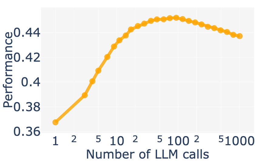
Figure 1: How the number of calls to GPT-3.5 affects its performance on the MMLU college mathematics dataset [HBB⁺20] when aggregating results via majority vote. We observe a surprising trend: at first, increasing the number of LLM calls improves accuracy, but later, it reduces it.

Compound AI systems that perform multiple Large Language Model (LLM) calls and aggregate their responses are increasingly leveraged to solve language tasks [ZKC⁺24, DLT⁺23, TAB⁺23, TWL⁺24, WWS⁺22]. For example, Google’s Gemini achieved state-of-the-art results on the MMLU benchmark using a CoT@32 voting strategy: the LLM is called 32 times, and then the majority vote of the 32 responses is used in the final response [TAB⁺23]. In addition to their superior performance, compound systems are appealing because they are convenient to construct and debug [ZKC⁺24].

A natural question is, thus, how does scaling the number of LLM calls affect the performance of such compound systems? This question is under-explored in research, but characterizing the scaling dynamics is crucial for researchers and practitioners to estimate how many LLM calls are needed for their applications and allocate computational resources aptly. Understanding these scaling dynamics is also helpful to understand the limits of compound inference strategies.

As a first step towards answering this question, we study the scaling properties of one-layer Voting Inference Systems, a particularly simple compound system that aggregates multiple proposed answers via majority vote, as in Gemini’s CoT@32. While the inference system design space is broad and other systems, such as AlphaCode 2 [Alp23], use more complex filtering and aggregation strategies, we focus on one-layer Voting Inference Systems for two reasons. First, they have already been used in real application, such as as Gemini’s CoT@32 strategy. Second, despite their simplicity, they exhibit nontrivial scaling properties. Specifically, although one might expect the performance of these Voting Inference Systems to monotonically increase as more LLM calls are invoked, we have identified a surprising phenomenon on several language tasks with these systems: growing the number of LLM calls initially improves performance but then degrades it, as shown in Figure 1.

This surprising effect motivates our theoretical study of one-layer Voting Inference Systems, which explains this non-monotone effect through the diversity of item difficulty in a given task (see Figure 2 and Theorem 1). At a high level, our results show that more LLM calls continuously lead to better performance on “easy” queries and worse performance on “hard” queries. When a task is some mixture of “easy” and “hard” queries, the non-monotone aggregate behavior emerges. Formally, a query is easy if a one-layer Voting Inference System with infinitely many LLM calls gives a correct answer and hard otherwise. Intuitively, the probability that one LLM call’s output is correct is higher than 0.5 for easy queries, and thus as the number of LLM calls goes to infinite, the probability of a Voting Inference System’s output being correct goes to 1. For hard queries, the probability of generating one correct answer from a randomly chosen LLM call is less than 0.5, and thus the probability of a Voting Inference System goes to 0 as the number of LLM calls goes to infinite. We derive a scaling law of Inference Systems that explicitly models item difficulties, and present an algorithm that lets users fit the scaling law’s parameters using a small number of samples. In experiments with GPT-3.5, we show that these algorithms can let us estimate the scaling law for various problems and identify the optimal number of calls to make to the LLM to maximize accuracy.

Figure 2: Performance breakdown on easy and hard items. As the number of LLM calls increases, the one-layer Voting Inference System performs increasingly better on easy items but increasingly worse on the hard items. The math dataset consists of 58% hard questions.

Our study on the one-layer Voting Inference Systems opens the door for understanding and leveraging scaling properties of compound AI systems. We study here mainly one-layer Voting Inference Systems that use a majority voting scheme to aggregate LLM generations, but many compound systems leverage different aggregation mechanisms designed for different tasks. For example, AlphaCode 2 uses test cases to filter the generation set down for code generation [Alp23], Medprompt adopts an LLM as a judge to select answers for medical question answering [NKM⁺23], and AlphaGeometry combines LLM calls with exact derivations from a symbolic engine [TWL⁺24]. The scaling laws of these systems will differ from one-layer Voting Inference Systems and remain an interesting open problem. Another interesting future direction is to estimate item difficulties accurately and vary the number of inference calls for each item type in a voting system.

This work shows that more LLM calls do not necessarily improve the performance of compound AI systems, and that it is possible, at least in some cases, to predict how the number of LLM calls affects AI systems’ performance and thus decide the optimal number of LLM calls for a given task. We are releasing the code and dataset evaluated in this paper, and hope to stimulate more research on the important but under-explored problem of scaling laws of compound AI systems.

2 Related Work

Neural Scaling Laws.

There has been extensive research on how the training parameters affect the performance of neural language models [KMH⁺20, SGS⁺22, BDK⁺21, MLP⁺23]. Among others, the model loss has been empirically shown to follow a power law as the number of model parameters and training tokens [KMH⁺20]. Researchers have also proposed theories to explain the empirical scaling laws [BDK⁺21]. By contrast, recent work has found that scaling up the model parameters leads to performance decay on certain tasks [MLP⁺23]. To the best of our knowledge, there is no study on how the number of LLM calls affects the performance of a compound system, which is complementary to scaling laws on training parameters and data set sizes.

Compound Systems using LLMs.

Many inference strategies that perform multiple model calls have been developed to advance performance on various language processing tasks [DLT⁺23, TAB⁺23, TWL⁺24, WWS⁺22, CZZ23, ZKAW23, ŠPW23]. For example, Gemini reaches state-of-the-art performance on MMLU via its CoT@32 majority voting scheme [TAB⁺23]. Self-consistency [WWS⁺22] boosts the performance of chain-of-thought via a majority vote scheme over multiple reasoning paths generated by PaLM-540B. Finally, AlphaCode 2 [Alp23] matches the 85th percentile of humans in a coding contest regime by generating up to one million samples per problem via an LLM and then filtering the answer set down. While these approaches are empirically compelling, there has been little systematic study of how the number of LLM calls affects these systems’ performance.

3 Definitions and Problem Statement

Let us start by presenting the generic framework of Voting Inference Systems, modeling item difficulty, and stating the problem of scaling properties.

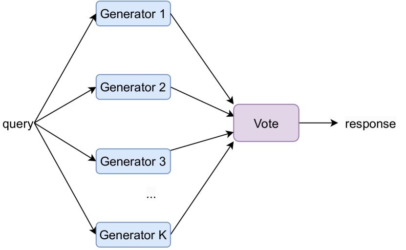
Figure 3: One-layer Inference Systems.

Input: A user query $x$

Output: A response $\hat{y}$

1 Sample $\theta_{1},\theta_{2},\cdots,\theta_{K}$ from $\Theta$;

2 Generate $z_{k}=G(x,\theta_{k}),k=1,2,\cdots,K$;

3 Compute $\hat{y}=\arg\max_{a\in A}\sum_{k=1}^{K}\mathbbm{1}_{z_{k}=a}$;

Return $\hat{y}$

Algorithm 1 One-layer Voting Inference System Pipeline.

3.1 Voting Inference Systems

In this paper, we focus on one-layer Voting Inference Systems, as depicted in Figure 3. Given a user query, a one-layer Voting Inference System (i) first generates multiple candidate answers, and (ii) then uses a majority voting scheme to choose one as the final response. The one-layer Voting Inference Systems are inspired and resemble several real-world compound AI systems, such as self-consistency [WWS⁺22], Medprompt [NKM⁺23], and Gemini CoT@32 strategy [TAB⁺23]. The details of the one-layer Voting Inference Systems are given in Algorithm 1, and we explain the generation and majority voting steps as follows.

Generation.

LLMs are probabilistic language models, and thus the generation phase of Inference Systems is also randomized: parameters $\theta_{1},\theta_{2},\cdots,\theta_{K}$ are first randomly drawn from some parameter distribution $\Theta$, and then for each $\theta_{k}$ and the query $x$, a deterministic generator $G$ is invoked to produce a candidate answer $z_{k}=G(x,\theta_{k})$. Here, instantiations of $\Theta$ are a design choice of users and can encode many generation strategies. For example, even with a single fixed LLM, diverse generations may be achieved by using a non-zero temperature and different prompt wordings or few-shot examples for each call to the LLM. If $\Theta$ contains different LLMs, then this system definition can also represent LLM ensembles. For ease of analysis, we assume $\theta_{1},\theta_{2},\cdots,\theta_{K}$ are i.i.d. drawn from $\Theta$ and thus all generations $z_{1},z_{2},\cdots z_{K}$ are also i.i.d. throughout the paper.

Majority Voting.

Given all candidate answers, the majority voting scheme works by choosing the mode among all candidate responses, that is $\hat{y}=\arg\max_{a\in A}\sum_{k=1}^{K}\mathbbm{1}_{z_{k}=a}$, where $A$ is the space of all possible answers. We break ties arbitrarily. This is directly applicable to tasks with a short answer space $A$, such as multiple-choice questions, classification, knowledge extraction, and single-line code completion.

3.2 Item Difficulty

How can we quantify the difficulty of a query item $x$ in an evaluation task? One natural option is correct answer rate, i.e., how likely a candidate answer is correct, denoted by $r(x)\triangleq\mathbb{E}_{\theta\sim\Theta}[G(x,\theta)=y]\in[0,1]$. Intuitively, large $r(x)$ indicates that the query $x$ is relatively easy to answer, and small $r(x)$ implies that it is hard. If $r(x)>0.5$, we call $x$ an “easy” query. Otherwise, we call it a “hard” query.

Now, we can quantify the difficulty of a data distribution $D$ by a distribution over the item difficulty, denoted by $\mathcal{P}$. That is, for an item $x$ randomly drawn from $D$, its difficulty $r(x)$ follows $\mathcal{P}$.

3.3 Problem Statement

Our goal is to study the scaling properties of one-layer Voting Inference Systems, i.e., how the number of LLM calls $K$ affects an Inference System’s performance on a data distribution $D$, denoted by $F(K;D)$. For exposure purposes, we focus on the expected $0/1$ loss as the performance metric, i.e., $F(K;D)=\mathbbm{E}[\hat{y}=y]$, where the expectation is taken over the data distribution $D$ and the sample parameters $\theta_{1},\theta_{2},\cdots,\theta_{K}$ in the Voting Inference System. Note that our analysis can generalize to other loss functions as well. For simplicity, let us also assume that the difficulty of items in $D$ takes values from only two values. More specifically, for a query $x\in D$,

$$r(x)=\begin{cases}p_{1},&\textit{ with probability }\alpha\\ p_{2},&\textit{ with probability }1-\alpha\\ \end{cases}$$

We say that such a $D$ is $2$-level difficult with parameter $(\alpha,p_{1},p_{2})$. W.L.O.G, let us assume $p_{1}>p_{2}$. We also suppose that the answer space $A$ contains only two possible answers. We will discuss how some of our results can be generalized to the generic difficulty distribution and answer space, but we leave an in-depth as future work.

Table 1: Notations.

Symbol	Meaning
$x$	an input query
$y$	the correct answer
$K$	the number of LLM calls
$z_{k}$	the output by one LLM call
$\hat{y}$	the output by a one-layer Voting Inference System
$D/D_{Tr}$	test dataset/train dataset
$A$	answer space
$\alpha$	fraction of easy queries
$p_{1}$	probability of $z_{k}$ being correct for easy queries
$p_{2}$	probability of $z_{k}$ being correct for hard queries
$F(K;D)$	Accuracy of the Voting Inference System with $K$ LLM calls on
$G(K;D)$	Scaling Approximation of $F(K;D)$

4 Scaling Properties of Voting Inference Systems

Now we analyze Voting Inference Systems with a focus on their scaling properties. In particular, we (i) characterize how item difficulty shapes the performance landscape, (ii) derive the optimal number of LLM calls as a function of the item difficulty, (iii) propose a scaling law, and (iv) present an algorithmic paradigm to estimate the scaling law parameters using a small number of samples. For ease of reference, we have listed all major notations in Table 1.

4.1 Item Difficulty Shapes Performance Landscape

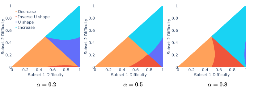
Figure 4: How the item difficulties shape the landscape of a one-layer Voting Inference System’s performance. Informally, if the overall task is “easy” ($p_{1}+p_{2}>1$), but the fraction of “hard” queries is large ($\alpha<1-\frac{1}{t}$), then as the number of LLM calls increases, the Voting Inference Systems’ performance increases first but then decreases. We call such a landscape a “inverse U shape”. Similarly, if the overall task is “hard” ($p_{1}+p_{2}<1$), but the fraction of “hard” queries is small ($\alpha>1-\frac{1}{t}$), then enlarging the number of LLM calls leads an initial decrease and then increase. Such a landscape is called a “U shape”. When $\alpha$ is large, the U-shape is less likely to occur while the inverse U-shape becomes more common. Smaller $\alpha$ leads to an opposite trend.

How does the item difficulty affect the performance landscape of a one-layer Voting Inference System? The following theorem gives a qualitative characterization.

Theorem 1.

Suppose $D$ is $2$-level difficult with $(\alpha,p_{1},p_{2})$, $\|A\|=2$, and $K$ is odd W.L.O.G. Let $t\triangleq\frac{p_{2}(1-p_{2})(\frac{1}{2}-p_{2})}{p_{1}(1-p_{1})(p_{1}-\frac{1}{2})}+1$. If $p_{1}+p_{2}\not=1$ and $p_{2}<\frac{1}{2}<p_{1}$, then as $K$ increases, $F(K;D)$

• increases monotonically, if $p_{1}+p_{2}>1$ and $\alpha\geq 1-\frac{1}{t}$

• decreases monotonically, if $p_{1}+p_{2}<1$ or $\alpha\leq 1-\frac{1}{t}$

• increases and then decreases, if $p_{1}+p_{2}>1$ and $\alpha<1-\frac{1}{t}$

• decreases and then increases, if $p_{1}+p_{2}<1$ and $\alpha>1-\frac{1}{t}$

Theorem 1 precisely connects the item difficulty with the performance landscape. Here, $t$ is a constant that only depends on $p_{1}$ and $p_{2}$, i.e., the probability of an LLM’s generation being correct on easy and hard queries, respectively. Intuitively, $t$ quantifies the difficulty similarity between the easy and hard queries: it becomes larger if the easy queries are more difficult ($p_{1}$ is smaller) or the hard queries are less difficult ($p_{2}$ is larger). Interestingly, it suggests that, for some item difficulty distribution, a non-monotone effect of the number of LLM calls is expected. Informally, if the overall task is “easy” ($p_{1}+p_{2}>1$), but the fraction of “hard” queries is large ($\alpha<1-\frac{1}{t}$), then as the number of LLM calls increases, the Voting Inference Systems’ performance increases first but then decreases. We call such a landscape a “inverse U shape”. Similarly, if the overall task is “hard” ($p_{1}+p_{2}<1$), but the fraction of “hard” queries is small ($\alpha>1-\frac{1}{t}$), then enlarging the number of LLM calls leads an initial decrease and then increase. Such a landscape is called a “U shape”. This well explains the U-shape of Inference Systems’ performance shown in Figure 1.Figure 4 visualizes the effects of item difficulty on the performance landscape in more detail.

4.2 Item Difficulty Determines Optimal Number of LLM Calls

We have shown that there are cases where, determined by item difficulty distribution, a non-monotone scaling behavior of Voting Inference Systems is expected. In these cases, blindly scaling up the number of LLM calls may not lead to the desired performance. How should one determine the number of LLM calls in these cases? The following result gives a precise answer.

Theorem 2.

Suppose $D$ is $2$-level difficult with $(\alpha,p_{1},p_{2})$, $\|A\|=2$, and $K$ is odd W.L.O.G. If $p_{1}+p_{2}>1$ and $\alpha<1-\frac{1}{t}$, then the number of LLM calls $K^{*}$ that maximizes the overall performance of an one-layer Voting Inference System(up to rounding) is

$$K^{*}=2\frac{\log\frac{\alpha}{1-\alpha}\frac{2p_{1}-1}{1-2p_{2}}}{\log\frac{p_{2}(1-p_{2})}{p_{1}(1-p_{1})}}$$

As expected, the optimal number of LLM calls depends on the item difficulty. For example, $K^{*}$ will be larger if $\alpha$ grows (up to $1-\frac{1}{t}$). That is, if there are more “easy” queries than “hard” queries, then a larger network should be adopted. This suggests that a difficulty-aware design of Voting Inference Systems may offer better performance than a difficulty-agnostic design. We will analyze $K^{*}$ in detail in Section 5.3.

4.3 A Scaling Law for One-layer Voting Inference Systems

We have seen that inference system performance is closely related to item difficulty. What is an intuitive way to explicitly model item difficulty in a scaling law of Voting Inference Systems? Here, we propose the following function $G(\cdot;\cdot)$ as a scaling law on the dataset $D$ with 2-level difficulty

$$G(K;D)\triangleq\alpha g_{p_{1}}(K;\boldsymbol{c}_{1})+(1-\alpha)g_{p_{2}}(K;\boldsymbol{c}_{2})$$

where

$$g_{p}(K;\boldsymbol{c})\triangleq\begin{cases}1-\exp(-\boldsymbol{c}^{T}[K,\sqrt{K},1])&\textit{if }p>\frac{1}{2}\\ \exp(-\boldsymbol{c}^{T}[K,\sqrt{K},1])&\textit{if }p<\frac{1}{2}\\ \end{cases}$$

This scaling law encodes how the item difficulty affects the performance. For example, if $p_{1}>\frac{1}{2}$ and $p_{2}<\frac{1}{2}$, the first term $g_{p_{1}}(\cdot;\cdot)$ will monotonically increase while the second term $g_{p_{2}}(\cdot;\cdot)$ will monotonically decrease, and hence the overall scaling function $G(K;D)$ exhibits a non-monotone behavior. This also captures that the number of LLM calls changes the performance at an exponential rate.

This scaling law can be easily generalized to data $D$ with generic item difficulty distribution. In particular, if the density function of the item difficulty is $q(u)$, then we can generalize the scaling law for the 2-level difficulty to this case via

$$G(K;D)\triangleq\int_{0}^{1}g_{q(u)}(K;\boldsymbol{c}_{u})q(u)du$$

For discrete distribution, one can simply replace the integral by summation and the density function by the mass function.

4.4 Estimating the Scaling Law Parameters

In practice, an important problem is to learn the scaling law using a small number of samples. Here, we give an algorithmic paradigm to estimate the scaling law parameters and thus the overall scaling function $G(\cdot;\cdot)$, as shown in Algorithm 2.

The estimation paradigm contains two major steps: it first estimates the scaling parameter for each item in the training dataset, and then aggregates the results to obtain the overall scaling function. To estimate the scaling law on each item, it first compares the majority vote on a few samples (line 2) with the true label to determine if the query is easy or not and thus selects the parametric form (line 3). Then it uses the empirically observed performance on a few samples to fit the parameters (line 4). For demonstration purposes, we use a square loss function as the optimization metric. Finally, the aggregation (line 5) over each item’s scaling function is returned as the final estimation.

Input: A training dataset $D_{Tr}=\{x_{i},y_{i},\{z_{i,m}\}_{k=1}^{K},\{F(t;\{x_{i}\})\}_{t\in T}\}_{i=1}^{n}$

Output: The scaling function $G(K)$

1 for $i=1$ to $n$ do

2      

      $\hat{y}_{i}=\arg\max_{a\in A}\sum_{m=1}^{M}\mathbbm{1}_{z_{i,j}=a}$ // Identify majority choices

       $G_{i}(K;\alpha)=\begin{cases}g_{0}(K;\alpha),&\textit{$y_{i}=\hat{y}_{i}$ }\\ g_{1}(K;\alpha),&o/w\end{cases}$// choose the parametric form

3      

      Obtain $\boldsymbol{c}_{i}=\arg\min_{\alpha}\sum_{t\in T}\ell(G_{i}(t;\alpha),F(t;\{x_{i}\}))$ // fit the parameter

4      

Return $G(K;D_{Tr})=\frac{1}{n}\sum_{i=1}^{n}G_{i}(K;\boldsymbol{c}_{i})$ // aggregate

Algorithm 2 Scaling Law Estimation

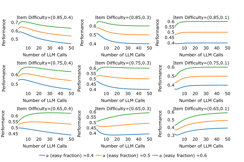
Figure 5: Overall performance of one-layer Voting Inference Systems on synthesized datasets with bi-level difficulty. Overall, we observe that increasing the number of LLM calls does not necessarily lead to performance improvements. For example, when the item difficulty is $(0.85,0.4)$, the performance increases first and then decreases as the number of LLM calls grows. When the item difficulty is $(0.65,0.1)$, there is a reverse trend: the performance goes down first and then goes up. This validates our empirical observation that a larger number of LLM calls and thus more resources may not necessarily result in better performance.

5 Experiments

We compare the empirical performance of one-layer Voting Inference System and the performance predicted by our analytical model. Our goal is three-fold: (i) validate that there are cases where increasing the number of LLM calls does not monotonically improve the performance of Inference System, (ii) justify that our scaling law can accurately predict Inference System’s performance and thus these cases, and (iii) demonstrate that our proposed scaling law can identify the optimal number of LLM calls correctly. Both synthetic and real-world datasets are used.

Datasets and LLM used by the one-layer Voting Inference Systems.

To understand the scaling properties of Voting Inference Systems, we conduct systematical experiments using (i) a simulated LLM on a synthesized dataset with controlled item difficulties, and (ii) a real LLM on real-world datasets. Specifically, for the simulated LLM, the synthesized dataset is of 2-level difficulty with parameters $(\alpha,p_{1},p_{2})$, and we study the scaling behavior by varying the parameters. For the real-world experiments, GPT-3.5-turbo-0125 is the LLM used by the one-layer Voting Inference Systems. All performance evaluation is averaged over 1,000 runs.

5.1 Increasing the Number of LLM Calls Can Help or Hurt Final Accuracy

We start by understanding how the item difficulty affects Voting Inference Systems’ performance landscape. For a systematic study, we create a dataset with a bi-level difficulty. We vary (i) the fraction of the easy subset $\alpha$ and (ii) the query difficulty on the easy and hard subset. When it is clear from the context, we may also call $(p_{1},p_{2})$ item difficulty. The performance of the Voting Inference Systems is shown in Figure 5.

Overall, we observe that item difficulty plays an important role in the number of LLM calls’ effects. For example, when the hardness parameter is $(0.85,0.1)$ and the fraction of easy queries is $\alpha=0.6$, Inference System’ performance is monotonically increasing as the number of LLM calls grows. However, adding more hard queries by changing the fraction $\alpha=0.4$ changes the trend: the performance goes down first for small call numbers and then goes up for larger numbers of calls. It is also interesting to notice an inverse “U”-shape. For example, when item difficulty is $(0.85,0.4)$, there is a clear U-shape performance. Overall, this implies that (i) there are cases where increasing the number of LLM calls is not beneficial, and (ii) item difficult is critically important to determine these cases.

5.2 Performance Estimation via Our Proposed Scaling Law

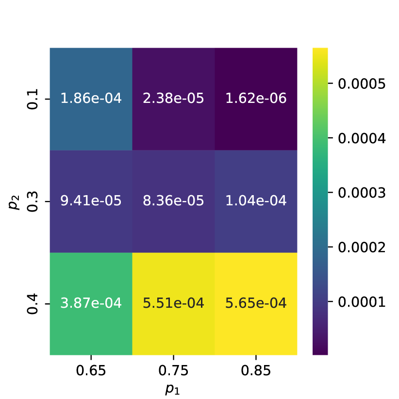
((a)) $\alpha=0.4$

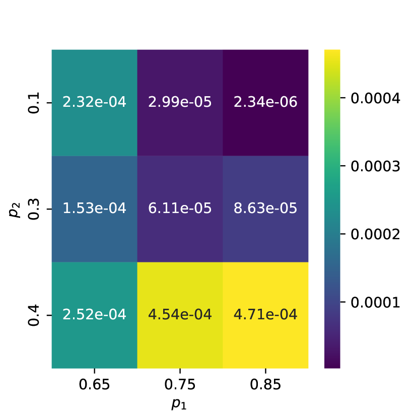
((b)) $\alpha=0.5$

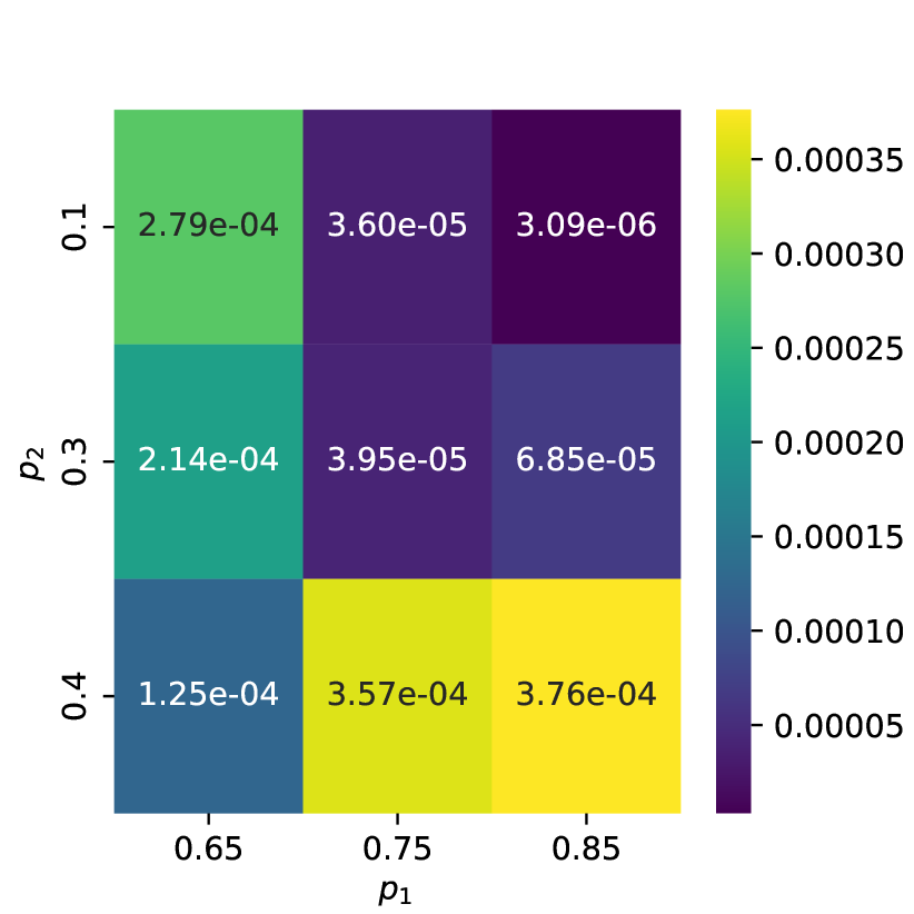
((c)) $\alpha=0.6$

Figure 6: Mean square error of the performance predicted by our proposed scaling law on synthesized datasets with varying bi-level difficulties. Here, we fit the scaling law by performance evaluated at $K=1,2,3,4,5$, and evaluate its performance for $K$ from 1 to 100. Overall, we observe that the predicted performance accurately matches the empirical evaluation.

Can our proposed scaling law predict the empirical performance of one-layer Voting Inference System accurately? To answer this, we apply our scaling law estimation to each dataset considered in Figure 5. In particular, we feed our estimator with the Inference Systems’ performance with number of LLM calls being $1,2,3,4,5$, and then uses it to predict the performance for LLM calls within the range from 1 to 100. Note that this is quite challenging, as the estimator needs to extrapolate, i.e., predict the performance of a Voting Inference System whose number of LLM calls is much larger than any number seen in the training data.

As shown in Figure 6, the performance predicted by our estimator accurately matches the empirical observation. Across all item difficulty parameters, the mean square error ranges from $1e-6$ to $1e-4$. This suggests that predicting how the number of LLM calls affects a Voting Inference System is feasible and also indicates that our scaling law captures the key performance trend effectively.

5.3 Finding the Optimal Number of LLM Calls

Table 2: Optimal number of LLM calls prediction. For each data distribution with specific 2-level difficulty parameters $\alpha,p_{1},p_{2}$, we sample 100 data points, employ a simulated Voting Inference System with 1000 number of LLM calls, estimate the parameters by their empirical mean and adopt the analytical optimal number of LLM calls predictor. Across evaluated item difficulties, our predicted optimal number of LLM calls exactly matches the optimal number empirically observed.

$\alpha$	$p_{1}$	$p_{2}$	$\hat{\alpha}$	$\hat{p}_{1}$	$\hat{p}_{2}$	Optimal Number of LLM Calls
						Analytical/Empirical
0.4	0.85	0.4	0.42	0.84	0.40	3
0.4	0.85	0.3	0.38	0.85	0.30	1
0.4	0.75	0.4	0.41	0.74	0.40	4
0.4	0.75	0.3	0.44	0.75	0.30	1
0.4	0.65	0.4	0.41	0.65	0.40	1
0.5	0.85	0.4	0.50	0.84	0.40	4
0.5	0.85	0.3	0.50	0.85	0.30	2
0.5	0.75	0.4	0.51	0.75	0.40	7
0.5	0.75	0.3	0.49	0.75	0.30	4
0.5	0.65	0.4	0.48	0.65	0.40	15
0.6	0.85	0.4	0.59	0.84	0.39	5
0.6	0.85	0.3	0.63	0.85	0.30	4
0.6	0.75	0.4	0.61	0.75	0.40	11
0.6	0.75	0.3	0.59	0.75	0.30	11
0.6	0.65	0.4	0.62	0.65	0.40	30

Identifying the optimal number of calls is an important implication of the scaling properties. Here, we compare the optimal number of calls predicted by our analytical model and the optimal numbers empirically observed. As summarized in Table 2, the predicted optimal number is exactly the observed optimal number of LLM calls, for all item difficulties evaluated. This validates the assumptions made by Theorem 2.

5.4 Scaling Properties on Real-world Datasets

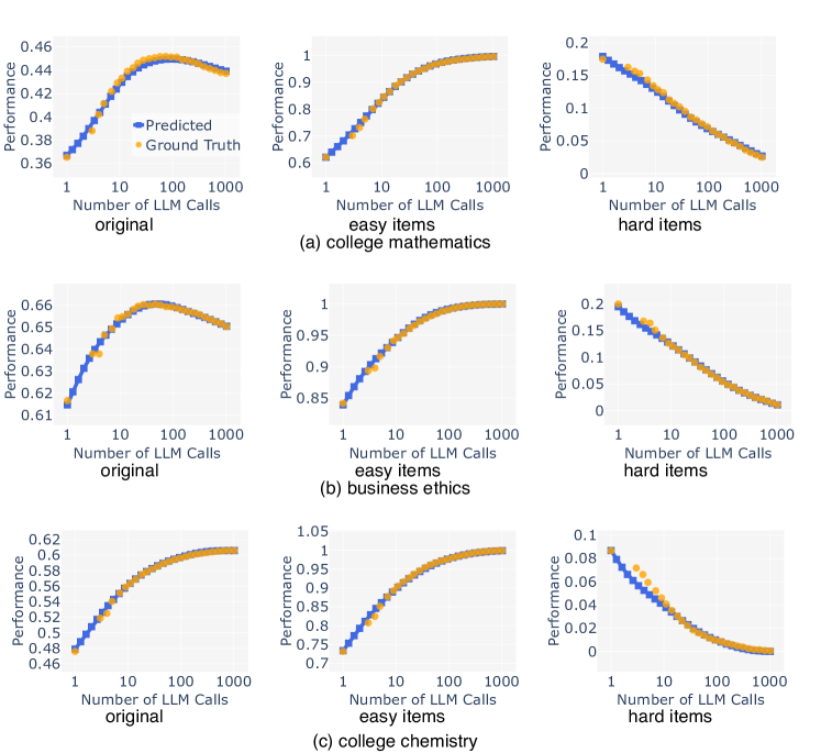
Figure 7: Inference System’s performance and our prediction on real-world datasets. The orange dots are the empirical performance of a one-layer Voting Inference System averaged over 1000 runs, and the blue lines correspond to the performance predicted by our scaling law. GPT-3.5-turbo-0125 is the LLM adopted by the one-layer Voting Inference System. Overall, we observe that increasing the number of calls does not always lead to performance gains. This is because its effects are opposite on the easy and hard queries. Our analytical model can accurately predict the performance and thus enables optimal ensemble size selection without an exhaustive search of all possible numbers of calls.

Finally, we validate the effectiveness of our scaling law on real-world datasets. We focus on three datasets as a first step: college mathematics, business ethics, and college chemistry, curated from the MMLU benchmark [HBB⁺20]. Each query in these datasets is a multiple-choice question. We use GPT-3.5 to generate candidate answers. For each generation, we add 1 to 2 few-shot examples randomly chosen from a pool of 5 examples to the prompt to encourage diversity. We set the temperature to be 0.7. Here, a query item is considered easy if the majority vote of 1,000 GPT-3.5’s generations is correct, and is considered difficult otherwise. To fit our scaling law, we use the performance evaluated with $1,10,100$ and $1000$ LLM calls as the training data, and then use the estimated scaling law to predict the performance for all other numbers of LLM calls.

Figure 7 shows the overall performance of one-layer Voting Inference System with varying numbers of LLM calls and also the performance predicted by our scaling law. There are several interesting observations. First, the overall performance is not always monotonically increasing as the number of LLM calls grows. On college mathematics and business ethics, for example, the performance is maximized at a specific number of LLM calls and becomes worse when the number of LLM calls becomes further away from this unique nubmer. Second, we observe that this counter-intuitive phenomenon can be explained by the performance breakdown on easy and hard subsets. In fact, on the easy subsets, the Voting Inference System’s performance monotonically increases as the more LLM calls are invoked. On the other hand, on the hard queries, the performance continuously decays as more LLM calls are invoked. This is also true even if the overall performance is monotone. For example, on the college chemistry dataset, increasing the number of LLM calls leads to a continuously improved overall performance, but also a continuously decreasing performance on the hard queries. This reveals a fundamental tradeoff: the number of LLM calls has opposite effects on easy and hard queries, and changing it balances performance on easy and hard queries. Furthermore, our scaling law can accurately predict the performance of Voting Inference System, on the full data, easy subset, and the hard subset. In practice, this makes it much easier to identify the optimal number of LLM calls: one can simply choose the number that maximizes the predicted performance.

5.5 Predicting Query Difficulty

Table 3: Zero-shot Difficulty Prediction Performance on real-world datasets. Overall, zero-shot GPT-4-turbo correctly recognizes the difficulty for a large range of queries, although there is still a large room for improvement.

LLM Predictor	College Mathematics	Business Ethics	College Chemistry
GPT-4	65.7%	67.6%	71.7%
GPT-3.5	58.6%	55.5%	51.5%
Dummy	57.6%	64.6%	60.6%

We also explore how accurately LLMs can infer the item difficulty. In a nutshell, we give an LLM a question item, the response by an Inference System, and asks the LLM whether the question is difficult to the Inference System. As a first step, we use GPT-4 and GPT-3.5 as the difficulty predictor, and evaluate their performance as shown in Table 3. Interestingly, GPT-3.5 performs poorly as its accuracy is on par with the dummy predictor, which gives the most frequent label (e.g., always “easy”). On the other hand, GPT-4 seems to predict the item difficulty reasonably well, with 3% to 11% improvement compared with the dummy predictor that always predicts the more common class.

Note that a high-quality difficulty predictor are practically valuable. For example, we can integrate it into a Inference System to enable fine-grained network size selection. If the query is predicted to be easy, use a large number of LLM calls. Otherwise, only call an LLM a few times. We leave designing high-quanlity difficulty predictors and principled ways to leverage the predictors as future work.

6 Discussion and Conclusion

In this paper, we systematically study how the number of LLM calls affects the performance of one-layer Voting Inference Systems, one of the simplest compound systems. Our main discovery is quite interesting: increasing the number of LLM calls engenders performance increase initially, but then performance decreases. We offer theoretical analysis that attributes this surprising phenomenon to the diversity of query difficulty, and conduct experiments to validate our analysis. Note that in this work, we do not discuss the cost of LLM calls; this is an important dimension to weigh in practice, and in future work we will investigate how to balance cost, performance, and latency scaling.

Our findings open the door to understanding how compound systems scale with the number of LLM calls, and pinpoint many interesting future directions to study. This study focuses on one-layer Voting Inference Systems, but there are many other types of inference systems and, more generally, compound systems. How other constructions scale remains an interesting and open question. For example, rather than a voting-based aggregation of LLM responses, a system could rank and select among responses. As a function of the quality of the ranking scheme, very different scaling dynamics can emerge – for example, a system based upon a perfect ranker that always selects the best response (e.g., by checking whether a generated mathematical proof is correct) would exhibit monotone scaling with the number of generations. Going forward, it is also of high practical value to further study how to accurately predict the difficulty of a given query.

Overall, our study shows that more LLM calls are not necessarily better and underscores the importance of compound system design. We hope our findings and analysis will inspire more research into maximally effective AI system construction.

Appendix A Useful Lemmas

Lemma 3.

Suppose $D$ is $2$-level difficult with $(\alpha,p_{1},p_{2})$ and $\|A\|=2$, and W.L.O.G, $K$ is odd. Then $F(K;D)=\alpha I_{p_{1}}(\frac{K+1}{2},\frac{K+1}{2})+(1-\alpha)I_{p_{2}}(\frac{K+1}{2},\frac{K+1}{2})$, where $I_{x}(a,b)\triangleq\int_{0}^{x}t^{a-1}(1-t)^{b-1}dt$ is the incomplete beta function.

Proof.

To analyze how the performance scales as the network size increases, let us first expand the performance of Inference System by the law of total expectation

$$F(K;D)=\mathbbm{E}[\hat{y}=y]=\sum_{i=1}^{2}\mathbbm{E}[\hat{y}=y|r(x)=p_{i}]\Pr[r(x)=p_{i}]$$ (A.1)

Now consider $\mathbbm{E}[\hat{y}=y|r(x)=p]$ for any $p$. Note that there are in total 2 possible generations (by $\|A\|=2$), so the estimated generation $\hat{y}$ is correct if and only if more than half of the generations is correct. That is to say, $\mathbbm{E}[\hat{y}=y|r(x)=p]=\Pr[\sum_{k=1}^{K}\mathbbm{1}_{z_{k}=y}>\frac{K}{2}]=1-\Pr[\sum_{k=1}^{K}\mathbbm{1}_{z_{k}=y}\leq\frac{K}{2}]$. For ease of notation, denote $Z\triangleq\sum_{k=1}^{K}\mathbbm{1}_{z_{k}=y}$. Note that $\mathbbm{1}_{z_{k}=y}$ is a Bernoulli variable with parameter $p$ and thus $Z$ is a Binomial variable with parameter $(K,p)$. Therefore, we have $Pr[Z\leq w]=I_{1-p}(K-w,w+1)$, where $I_{x}(a,b)\triangleq\int_{0}^{x}t^{a-1}(1-t)^{b-1}dt$ is the incomplete beta function. Thus, the above gives us

$$\mathbbm{E}[\hat{y}=y|r(x)=p]=1-I_{1-p}(K-\lfloor\frac{K}{2}\rfloor,\lfloor\frac{K}{2}\rfloor+1)=I_{p}(\lfloor\frac{K}{2}\rfloor+1,K-\lfloor\frac{K}{2}\rfloor)$$

If $K$ is odd, we can write it as $mathbbm{E}[\hat{y}=y|r(x)=p]=I_{p}(\frac{K+1}{2},\frac{K+1}{2})$ We can now plug this back into equation (A.1) to obtain

$$F(K;D) =\sum_{i=1}^{2}\mathbbm{E}[\hat{y}=y|r(x)=p_{i}]\Pr[r(x)=p_{i}]=\sum_{i=1}^{2}I_{p_{i}}(\frac{K+1}{2},\frac{K+1}{2})\Pr[r(x)=p_{i}]$$

$$=\alpha I_{p_{1}}(\frac{K+1}{2},\frac{K+1}{2})+(1-\alpha)I_{p_{2}}(\frac{K+1}{2},\frac{K+1}{2})$$

which completes the proof. ∎

Lemma 4.

$I_{p}(M+1,M+1)=I_{p}(M,M)+\frac{p^{M}(1-p)^{M}}{MB(M,M)}(2p-1)$, where $B(a,b)\triangleq\int_{0}^{1}t^{a-1}(1-t)^{b-1}dt$ is the beta function.

Proof.

Noting that $I_{p}(a+1,b)=I_{p}(a,b)-\frac{p^{a}(1-p)^{b}}{aB(a,b)}$, we have

$$I_{p}(M+1,M+1)=I_{p}(M,M+1)-\frac{p^{M}(1-p)^{M+1}}{MB(M,M+1)}$$

By $I_{p}(a,b+1)=I_{p}(a,b)+\frac{p^{a}(1-p)^{b}}{bB(a,b)}$, we have

$$I_{p}(M,M+1)=I_{p}(M,M)+\frac{p^{M}(1-p)^{M}}{MB(M,M)}$$

Thus, $I_{p}(M+1,M+1)=\frac{p^{M}(1-p)^{M}}{MB(M,M)}-\frac{p^{M}(1-p)^{M+1}}{MB(M,M+1)}$. The Pascal’s identity implies that $B(a,b+1)=\frac{a}{a+b}B(a,b)$ and thus $B(M,M+1)=B(M,M)/2$. Thus, we have

$$I_{p}(M+1,M+1)=\frac{p^{M}(1-p)^{M}}{MB(M,M)}-\frac{p^{M}(1-p)^{M+1}}{MB(M,M+1)}=\frac{p^{M}(1-p)^{M}}{MB(M,M)}-\frac{2p^{M}(1-p)^{M+1}}{MB(M,M)}$$

Extracting the common factors gives

$$\frac{p^{M}(1-p)^{M}}{MB(M,M)}-\frac{2p^{M}(1-p)^{M+1}}{MB(M,M)}=\frac{p^{M}(1-p)^{M}}{MB(M,M)}[1-2(1-p)]=\frac{p^{M}(1-p)^{M}}{MB(M,M)}(2p-1)$$

That is, $I_{p}(M+1,M+1)=I_{p}(M,M)+\frac{p^{M}(1-p)^{M}}{MB(M,M)}(2p-1)$, which completes the proof. ∎

Appendix B Proof of Theorem 1

Proof.

We construct a recurrent relation on $F(K;D)$ by Applying Lemma 3

$$F(K+2;D)-F(K;D)$$

$$= \alpha I_{p_{1}}(\frac{K+3}{2},\frac{K+3}{2})+(1-\alpha)I_{p_{2}}(\frac{K+3}{2},\frac{K+3}{2})-[\alpha I_{p_{1}}(\frac{K+1}{2},\frac{K+1}{2})+(1-\alpha)I_{p_{2}}(\frac{K+1}{2},\frac{K+1}{2})]$$

$$= \alpha(I_{p_{1}}(\frac{K+3}{2},\frac{K+3}{2})-I_{p_{1}}(\frac{K+1}{2},\frac{K+1}{2}))+(1-\alpha)(I_{p_{2}}(\frac{K+3}{2},\frac{K+3}{2})-I_{p_{2}}(\frac{K+1}{2},\frac{K+1}{2}))$$

For ease of notation, let us denote $M=\frac{K+1}{2}$. Applying Lemma 4 leads to

$$F(K+2;D)-F(K;D)$$

$$= \alpha[\frac{p_{1}^{M}(1-p_{1})^{M}}{MB(M,M)}(2p_{1}-1)]+(1-\alpha)[\frac{p_{2}^{M}(1-p_{2})^{M}}{MB(M,M)}(2p_{2}-1)]$$

$$= \frac{1}{MB(M,M)}[\alpha\cdot p_{1}^{M}(1-p_{1})^{M}(2p_{1}-1)+(1-\alpha)\cdot p_{2}^{M}(1-p_{2})^{M}(2p_{2}-1)]$$

Now rearranging the terms gives

$$F(K+2;D)-F(K;D)$$

$$= \frac{1}{MB(M,M)}\cdot(1-\alpha)p_{2}^{M}(1-p_{2})^{M}(1-2p_{2})\cdot[\frac{\alpha(2p_{1}-1)}{(1-\alpha)(1-2p_{2})}[\frac{p_{1}(1-p_{1})}{p_{2}(1-p_{2})}]^{M}-1]$$

For ease of notation, denote $\Delta F(M)\triangleq\frac{\alpha(2p_{1}-1)}{(1-\alpha)(1-2p_{2})}\frac{p_{1}(1-p_{1})}{p_{2}(1-p_{2})}]^{M}-1$. Note that $\Delta F(M)$ is monotonically increasing or decreasing, depending on the parameters $p_{1},p_{2}$. It is also easy to show that $\alpha\geq 1-\frac{1}{t}$ if and only if $\Delta F(1)\geq 0$. Now, we are ready to derive the main results by analyzing $\Delta F(M)$.

• $p_{1}+p_{2}>1$ and $\alpha\geq 1-\frac{1}{t}$: Now $\frac{p_{1}(1-p_{1})}{p_{2}(1-p_{2})}>1$, and thus $\Delta F(M)$ is monotonically increasing. Furthermore, it is easy to see $\lim_{M\rightarrow\infty}\Delta F(M)=\infty$. Furthermore, $\Delta F(1)\geq 0$. That is, for any given $M$, $\Delta F(M)$ is non-negative and thus $F(K;D)$ must be monotonically increasing

• $p_{1}+p_{2}>1$ and $\alpha<1-\frac{1}{t}$: Now $\frac{p_{1}(1-p_{1})}{p_{2}(1-p_{2})}>1$, and thus $\Delta F(M)$ is monotonically increasing. Furthermore, it is easy to see $\lim_{M\rightarrow\infty}\Delta F(M)=\infty$. Furthermore, $\Delta F(1)<0$. That is, as $K$ and thus $M$ increases, $\Delta F(M)$ is negative and then becomes positive. Therefore, $F(K;D)$ must decrease and then increase

• $p_{1}+p_{2}<1$ and $\alpha>1-\frac{1}{t}$: Now $\frac{p_{1}(1-p_{1})}{p_{2}(1-p_{2})}<1$, and thus $\Delta F(M)$ is monotonically decreasing. Furthermore, it is easy to see $\lim_{M\rightarrow\infty}\Delta F(M)=-1$. Furthermore, $\Delta F(1)>0$. That is, as $K$ and thus $M$ increases, $\Delta F(M)$ is positive and then becomes negative. Therefore, $F(K;D)$ must increase and then decrease

• $p_{1}+p_{2}<1$ and $\alpha\leq 1-\frac{1}{t}$: Now $\frac{p_{1}(1-p_{1})}{p_{2}(1-p_{2})}<1$, and thus $\Delta F(M)$ is monotonically decreasing. Furthermore, it is easy to see $\lim_{M\rightarrow\infty}\Delta F(M)=-1$. Furthermore, $\Delta F(1)\leq 0$. That is, for any given $M$, $\Delta F(M)$ is non-positive and thus $F(K;D)$ must be monotonically decreasing

Thus, we complete the proof. ∎

Appendix C Proof of Theorem 2

Proof.

Note that the optimal number of LLM calls must ensure that the incremental component $\Delta F(M)=0$. That is, the optimal value $M^{*}$ must satisfy $\Delta F(M^{*})=\frac{\alpha(2p_{1}-1)}{(1-\alpha)(1-2p_{2})}[\frac{p_{1}(1-p_{1})}{p_{2}(1-p_{2})}]^{M^{*}}-1=0.$ Solving the above equation gives us a unique solution

$$M^{*}=2\frac{\log\frac{\alpha}{1-\alpha}\frac{2p_{1}-1}{1-2p_{2}}}{\log\frac{p_{2}(1-p_{2})}{p_{1}(1-p_{1})}}$$

Noting that $K^{*}=\lceil 2M\rceil]$ completes the proof. ∎

References

- [Alp23] AlphaCode. Alphacode 2 technical report. https://storage.googleapis.com/deepmind-media/AlphaCode2/AlphaCode2_Tech_Report.pdf, 2023.
- [BDK+21] Yasaman Bahri, Ethan Dyer, Jared Kaplan, Jaehoon Lee, and Utkarsh Sharma. Explaining neural scaling laws. arXiv preprint arXiv:2102.06701, 2021.
- [CZZ23] Lingjiao Chen, Matei Zaharia, and James Zou. Frugalgpt: How to use large language models while reducing cost and improving performance. arXiv preprint arXiv:2305.05176, 2023.
- [DLT+23] Yilun Du, Shuang Li, Antonio Torralba, Joshua B Tenenbaum, and Igor Mordatch. Improving factuality and reasoning in language models through multiagent debate. arXiv preprint arXiv:2305.14325, 2023.
- [HBB+20] Dan Hendrycks, Collin Burns, Steven Basart, Andy Zou, Mantas Mazeika, Dawn Song, and Jacob Steinhardt. Measuring massive multitask language understanding. arXiv preprint arXiv:2009.03300, 2020.
- [KMH+20] Jared Kaplan, Sam McCandlish, Tom Henighan, Tom B Brown, Benjamin Chess, Rewon Child, Scott Gray, Alec Radford, Jeffrey Wu, and Dario Amodei. Scaling laws for neural language models. arXiv preprint arXiv:2001.08361, 2020.
- [MLP+23] Ian R McKenzie, Alexander Lyzhov, Michael Pieler, Alicia Parrish, Aaron Mueller, Ameya Prabhu, Euan McLean, Aaron Kirtland, Alexis Ross, Alisa Liu, et al. Inverse scaling: When bigger isn’t better. arXiv preprint arXiv:2306.09479, 2023.
- [NKM+23] Harsha Nori, Nicholas King, Scott Mayer McKinney, Dean Carignan, and Eric Horvitz. Capabilities of gpt-4 on medical challenge problems. arXiv preprint arXiv:2303.13375, 2023.
- [SGS+22] Ben Sorscher, Robert Geirhos, Shashank Shekhar, Surya Ganguli, and Ari Morcos. Beyond neural scaling laws: beating power law scaling via data pruning. Advances in Neural Information Processing Systems, 35:19523–19536, 2022.
- [ŠPW23] Marija Šakota, Maxime Peyrard, and Robert West. Fly-swat or cannon? cost-effective language model choice via meta-modeling. arXiv preprint arXiv:2308.06077, 2023.
- [TAB+23] Gemini Team, Rohan Anil, Sebastian Borgeaud, Yonghui Wu, Jean-Baptiste Alayrac, Jiahui Yu, Radu Soricut, Johan Schalkwyk, Andrew M Dai, Anja Hauth, et al. Gemini: a family of highly capable multimodal models. arXiv preprint arXiv:2312.11805, 2023.
- [TWL+24] Trieu H Trinh, Yuhuai Wu, Quoc V Le, He He, and Thang Luong. Solving olympiad geometry without human demonstrations. Nature, 625(7995):476–482, 2024.
- [WWS+22] Xuezhi Wang, Jason Wei, Dale Schuurmans, Quoc Le, Ed Chi, Sharan Narang, Aakanksha Chowdhery, and Denny Zhou. Self-consistency improves chain of thought reasoning in language models. arXiv preprint arXiv:2203.11171, 2022.
- [ZKAW23] Jieyu Zhang, Ranjay Krishna, Ahmed H Awadallah, and Chi Wang. Ecoassistant: Using llm assistant more affordably and accurately. arXiv preprint arXiv:2310.03046, 2023.
- [ZKC+24] Matei Zaharia, Omar Khattab, Lingjiao Chen, Jared Quincy Davis, Heather Miller, Chris Potts, James Zou, Michael Carbin, Jonathan Frankle, Naveen Rao, and Ali Ghodsi. The shift from models to compound ai systems. https://bair.berkeley.edu/blog/2024/02/18/compound-ai-systems/, 2024.