From Zero to Hero: How local curvature at artless initial conditions leads away from bad minima

Abstract

We investigate the optimization dynamics of gradient descent in a non-convex and high-dimensional setting, with a focus on the phase retrieval problem as a case study for complex loss landscapes. We first study the high-dimensional limit where both the number $M$ and the dimension $N$ of the data are going to infinity at fixed signal-to-noise ratio $\alpha=M/N$. By analyzing how the local curvature changes during optimization, we uncover that for intermediate $\alpha$, the Hessian displays a downward direction pointing towards good minima in the first regime of the descent, before being trapped in bad minima at the end. Hence, the local landscape is benign and informative at first, before gradient descent brings the system into an uninformative maze. The transition between the two regimes is associated to a BBP-type threshold in the time-dependent Hessian. Through both theoretical analysis and numerical experiments, we show that in practical cases, i.e. for finite but even very large $N$, successful optimization via gradient descent in phase retrieval is achieved by falling towards the good minima before reaching the bad ones. This mechanism explains why successful recovery is obtained well before the algorithmic transition corresponding to the high-dimensional limit. Technically, this is associated to strong logarithmic corrections of the algorithmic transition at large $N$ with respect to the one expected in the $N\to\infty$ limit. Our analysis sheds light on such a new mechanism that facilitate gradient descent dynamics in finite large dimensions, also highlighting the importance of good initialization of spectral properties for optimization in complex high-dimensional landscapes.

Keywords: Machine Learning $|$ Phase Retrieval $|$ Statistical Physics $|$ Non-convex Optimization

1 Introduction

Minimization of non-convex and high-dimensional landscapes with possibly many minima is routinely performed in machine learning and optimization with great success by means of basic local iterative procedures like gradient descent or its stochastic variants. Understanding why, and to what extent, these procedures work is an open challenge, to which a lot of studies were devoted recently. Without the aim of being exhaustive these include [41, 7, 27, 49, 33, 35, 1]. Several works have shown that actually spurious local minima are not present in certain regimes of parameters, e.g., when the signal-to-noise ratio is large enough [46, 11]. So, despite their non-convexity, landscapes can become easy to descend. This would suggest an explanation of the success of gradient descent optimization based on the ”trivialization” of the loss landscape [19], and the absence of bad minima. However, this cannot be the whole story, as it is known that bad minima are present in the regime of parameters where optimization succeeds [5, 23]. Theoretically, the study of gradient descent for matrix-tensor PCA [29], and later phase retrieval [31], offered a possible explanation. It showed that despite the presence of an exponential number (in the dimension $N$) of bad minima, the dynamics can avoid them with probability one. The mechanism is related to the complexity of the loss landscape: what matters is when the bad minima with the largest basins of attraction become unstable towards the good ones, not when all the bad ones disappear. This ”blessing” of dimension is due to the fact that the largest basin of attraction contain the initial conditions with probability one (up to corrections which are exponentially small in the dimension).

This work is devoted to another property of complex landscapes: how the local curvature evolves during the dynamics, and how this affects optimization. Following [31], we focus on phase retrieval as a model for high-dimensional landscape, and on gradient flow as optimization dynamics. We characterize the evolution of the spectral properties of the Hessian during the dynamics, and show the emergence of a new phenomenon associated to the complexity of high-dimensional landscapes which is crucial to characterize gradient descent dynamics.

Phase retrieval

The phase retrieval problem aims to recover a signal, $\bm{w}^{*}\in\mathbb{R}^{N}$, from the observation of $M$ absolute projections of sensing vectors $\bm{x}_{i}\in\mathbb{R}^{N}$ over it, $\{|y_{i}|\}_{i=1}^{M}$, with $y_{i}=\bm{x}_{i}^{\mkern-1.5mu\mathsf{T}}\bm{w}^{*}$. In our setting, the signal is considered to be drawn on the $N$-sphere with $\lVert\bm{w}^{\star}\rVert_{2}=\sqrt{N}$ and the sensing vectors $\{\bm{x}_{i}\}_{i=1}^{M}$ are considered i.i.d. Gaussian with zero mean and unit variance. Despite its simplistic formulation, this problem appears in various scientific fields ranging from quantum chromodynamics to astrophysics [38, 21, 36, 45, 17, 53] and is known to be NP-hard in general [42]. This complexity led researchers to develop numerous algorithms relying on diverse approaches over the previous decade [14, 40, 50, 16, 57, 51, 52, 56].

A natural way of estimating a candidate vector $\hat{\bm{w}}$ in the absence of any prior information is to specify a loss function $\ell(y_{i},\hat{y}_{i})$ and optimize it iteratively through a gradient descent procedure starting from a random location in the parameter space, namely

$$\hat{\bm{w}}^{(t+1)} =\hat{\bm{w}}^{(t)}-\eta\nabla_{\bm{w}}\mathcal{L}(\bm{w})+\eta\mu^{(t)}\hat{\bm{w}}^{(t)},$$ (1)

$$\mathcal{L}(\bm{w}) =\frac{1}{2}\sum_{i=1}^{M}\ell(y_{i},\hat{y}_{i}),$$ (2)

where $\eta$ is a fixed learning rate, $\hat{y}_{i}=\bm{x}_{i}^{\mkern-1.5mu\mathsf{T}}\bm{w}$ is the $i$^th estimated labels and $\mu^{(t)}=\hat{\bm{w}}^{(t)}\cdot\nabla\mathcal{L}(\bm{w}^{(t)})/N$ encodes the spherical constraint at each time step. Unless otherwise specified, the initial state is a random Gaussian vector, $\hat{\bm{w}}^{(0)}\sim\mathcal{N}(\bm{0}_{N},\bm{I}_{N})$. The phase retrieval problem can be seen as a single-layered neural networks with one output neuron and a square activation function.

Teacher-student

Our analysis is performed in the teacher-student setup. One network, the teacher, generates a set of $M$ measurements $\{y_{i}\}_{i=1}^{M}$ using a signal $\bm{w}^{\star}\sim\mathcal{N}(\bm{0}_{N},\bm{I}_{N})$. A second network with the same architecture, the student, exploits these measurements to estimate $\bm{w}^{\star}$ based on the procedure described by Eqs. (1) and (2). We are interested in the generalization ability of the student as measured by the overlap $m(t)=\hat{\bm{w}}^{(t)}\cdot\bm{w}^{\star}/N$ taking value one when it produces an estimate $\hat{\bm{w}}^{(t)}$ generalizing perfectly to new samples. It has been shown that for $\alpha=M/N<\alpha_{\mathrm{WR}}=0.5$, no estimator is able to obtain a generalization error better than a random guess while perfect recovery is achievable with the approximate message passing algorithm for $\alpha>1.13$ [6]. Although there are various forms of loss functions studied in the literature for the minimization of Eq. (2), we focus here on a normalized version of the intensity loss function defined as

$$\ell_{a}(y_{i},\hat{y}_{i})=\frac{\left(y_{i}^{2}-\hat{y}_{i}^{2}\right)^{2}}{\left(a+y_{i}^{2}\right)}.$$ (3)

The role played by the normalization is important for the conditioning of Hessian eigenspectrum, in particular ensuring the existence of a hard left edge, a crucial element of our analysis. Although the precise values at which the transitions occur may vary with the choice of the loss function, we expect the physical mechanisms at hand and the interpretation we propose in this paper to generalize well to other loss functions. While the main text focuses on $a=1$, we provide evidences by studying losses corresponding to different values of $a$ in Appendix D.

Further prior works

Many of the popular optimization methods developed over the past years rely on a careful initialization followed by an iterative algorithm in a form similar to Eq. (1). Such an initial guess is often provided by the leading eigenvector of a matrix function of the input data. This setup was studied in detail by [26] and [39] to identify the optimal pre-processing matrix producing a non-zero overlap between its leading eigenvector and the signal. In parallel, several works have thoroughly investigated whether it is possible to retrieve the signal efficiently based on a random initialization. [47] show that when the entries are i.i.d. Gaussian, a number of $O(N\log^{3}N)$ samples trivializes the landscape making all minima become global, hence enabling traditional iterative methods to find a solution independently of the initialization. This threshold was later reduced to $O(N)$ in [22, 12, 11] by adapting the form of the loss function, reducing the gap with the information-theoretic threshold of $M=N$.

By resorting to analogies with glassy dynamics of disordered systems, [31] argue that the convergence of a gradient descent algorithm is related to the trivialization of only a subset of bad minima. The dynamics is first trapped into peculiar high-energy minima, commonly called a threshold states in the physics literature. When $\alpha$ is large enough, these states develop a negative direction and a second descent phase occurs throughout a locally convex basin until a global minimum is reached, hence converging to $\pm\bm{w}^{\star}$. The transition between the two phases is governed by an eigenvalue popping out of the continuous bulk of the otherwise-marginal Hessian spectrum. This phenomenon is called a Baik-Ben Arous-Péché (BBP) transition [4] and was also observed in other optimization problems [29, 32].

The teacher-student setting that we study here is a particular case of learning a single-index model in which we assume the activation function of the teacher to be known to the student. These models received much attention these past years [3, 8, 9, 2, 10], essentially to understand the dynamics of (online) stochastic gradient descent in the loss landscape.

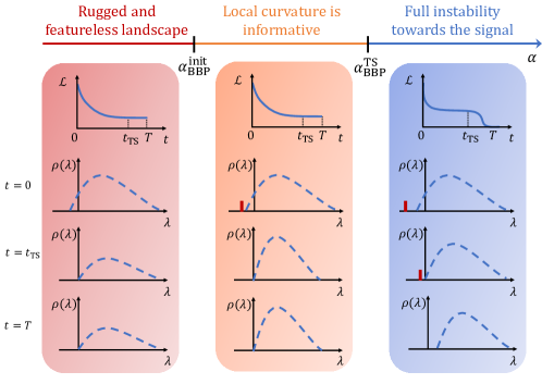
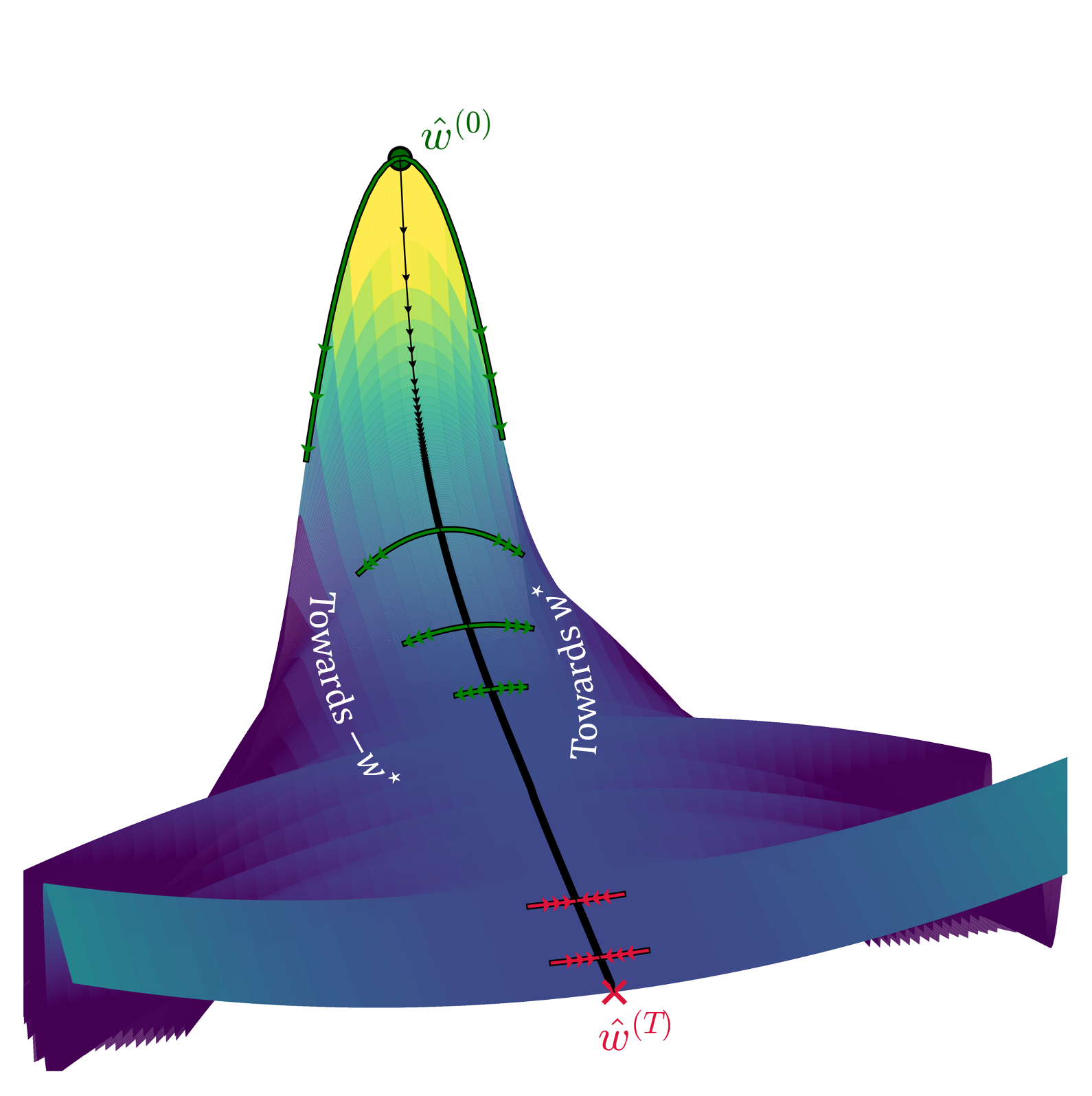
Figure 1: (Left) Phases of the gradient descent dynamics in the phase retrieval loss landscape for $N\rightarrow\infty$. (Right) Evolution of the local curvature: dynamics projected in the direction of least stability of the Hessian matrix (black arrows) for $\alpha=2\in\left[\alpha_{\mathrm{BBP}}^{\mathrm{init}}=1.13;\alpha_{\mathrm{BBP}}^{\mathrm{TS}}=6.55\right]$ and $N=256$. Starting from a random initial state $\hat{\bm{w}}^{(0)}$, gradient descent moves towards a threshold state at time $T$ that contains no information about the signal. The green arrows indicate downward directions towards the signal $\pm\bm{w}^{\star}$ with a decreasing amplitude as the descent goes. At $T$ the curvature has become positive. This description, valid for $N\rightarrow\infty$, drastically changes at finite $N$: the system benefits from the negative local curvature and starts to descend towards the signal well before $\alpha_{\mathrm{BBP}}^{\mathrm{TS}}$.

Contributions

We investigate the change in the spectral properties of the loss Hessian during gradient descent dynamics, in the high-dimensional regime $N,M\to\infty$ at fixed ratio $\alpha=M/N$. We show the existence of different regimes depending on the value of $\alpha$, that we summarize in the left panel of Fig. 1:

1. Rugged and featureless landscape: When $\alpha<\alpha_{\mathrm{BBP}}^{\mathrm{init}}$, the initial Hessian does not carry any information about the signal. Gradient descent initialized randomly is unable to find the signal and gets stuck into high-loss minima that are marginally stable (i.e., with a vanishingly small eigenvalue) called threshold states;

2. Local curvature is informative: When $\alpha\in\left[\alpha_{\mathrm{BBP}}^{\mathrm{init}};\alpha_{\mathrm{BBP}}^{\mathrm{TS}}\right]$, any initial condition sits in a region of the landscape with a downward direction pointing towards the signal. However, this direction is not the one followed by gradient descent. Instead, the dynamics gets once again trapped into a minimum (a threshold state) that does not generalize well. The initial information is therefore lost during the descent, as illustrated in the right panel of Fig. 1.

3. Full instability towards the signal: When $\alpha>\alpha_{\mathrm{BBP}}^{\mathrm{TS}}$, the threshold states turn from local minima to saddle-points that have exactly one negative direction pointing towards the signal, making gradient descent converge to a well-generalizing (global) minimum.

These findings have important consequences for finite but large dimensions, as we show later. In regime 2 the local curvature towards the good minima is negative at the beginning of the dynamics and positive at the very end (see right panel of Fig. 1). In this case, for any finite but large dimension, the system can descend along the negative curvature and recover the signal before the algorithmic transition taking place at $\alpha_{\mathrm{BBP}}^{\mathrm{TS}}$. We expect that this effect disappears for $N\rightarrow\infty$, as the system takes a time of order $\log N$ to escape the equator (defined as the set of states $\hat{\bm{w}}$ with zero overlap with the signal). Hence, before being able to escape, the system gets trapped in the threshold states for $\alpha<\alpha_{\mathrm{BBP}}^{\mathrm{TS}}$. Nevertheless, for finite and even very large $N$, this phenomenon is at play and disappears only logarithmically with $N$ (i.e., it should lead to an effective algorithmic transition growing with $\log N$). It is therefore very relevant for practical applications and explains the large gap reported in [31] between the value of $\alpha$ computed analytically and the empirical success rates obtained from numerical simulations. It also highlights the importance of a good initialization for optimization in high-dimensional non-convex landscapes, in particular by spectral methods (the Hessian initialization being a particular case). In order to find this effect, it was crucial to study a model with a complex landscape such as phase retrieval since it is not present in simpler problems like the matrix-tensor PCA [30].

Our results are established by a detailed analytical study of the spectral properties of the Hessian, in particular the associated BBP transition (presented in Sect. 3) and confirmed by suitably designed numerical experiments in Sect. 4.

Reproducibility

The code used to run the simulations and produce the figures will be made available upon acceptance.

2 A motivating example

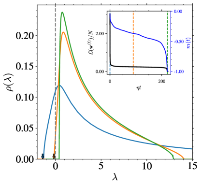
Figure 2: Hessian eigenvalues of a successful simulation with $N=2048$, $\alpha=3.1$, and $a=1$. The inset shows the evolution of the rescaled loss function $\mathcal{L}(\bm{w}^{(t)})/N$ and the overlap $m(t)=\bm{w}^{(t)}\cdot\bm{w}^{\star}/N$. Colored lines refer to different times shown in the inset. Arrows indicates the minimum eigenvalue when it is isolated from the bulk.

To illustrate the phenomenon we will analyze later, let us first describe a numerical example of a trajectory in regime 2. Figure 2 shows the evolution of the eigenspectrum at several timesteps during a successful realization of gradient descent initialized randomly for $\alpha=3.1$ with the loss function $\ell_{a=1}$. The inset highlights two phases: First, the loss function quickly decreases to reach a plateau in which the system gets stuck for most of the simulation time. Second, a descent phase where it finally escapes the saddle-point and the loss reaches zero. While the system iteratively moves towards a low loss value, the Hessian displays a single negative eigenvalue in the direction of the signal (blue and orange arrows). As the local curvature towards the signal is negative from the beginning of the dynamics, the system exploits this direction and eventually reaches a global minimum with all positive eigenvalues (green curve) and an overlap $m(T)=-1$, before getting trapped in the threshold states that would be stable at this value of $\alpha$. More details on the evolution of $m(t)$, shown in the inset, will be discussed at the end of Sect. 3.

3 Theory of the BBP transitions in the descent of the phase retrieval loss landscape

3.1 Method: Hessian eigenspectrum and BBP condition

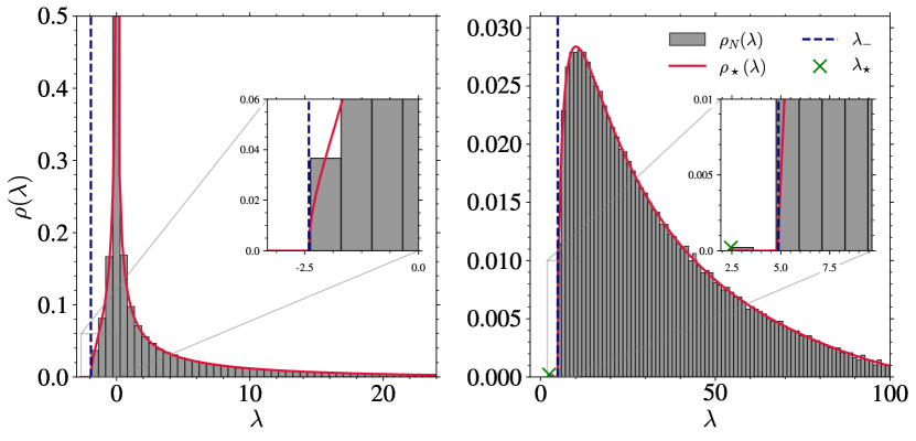
Figure 3: Illustrative comparison of the eigenspectrum properties analytically predicted from Eqs. (5), (8), and (9) with empirical spectra. Eigenvalues are obtained at $t=0$ (initialization) for $N=4096$, $a=1$, and (Left) $\alpha=1$ or (Right) $\alpha=10$.

The Hessian matrix associated to the minimization of Eq. (2) is of the form

$$\mathcal{H}(\bm{w})=\sum_{i=1}^{M}f_{i}\bm{x}_{i}\bm{x}_{i}^{\mkern-1.5mu\mathsf{T}}-\mu\bm{I}_{N},$$ (4)

with $f_{i}=\partial^{2}_{\hat{y}_{i}}\ell_{a}(y_{i},\hat{y}_{i})$, and $\bm{I}_{N}$ the identity matrix of size $N\times N$. In what follows, we omit the spherical constraint without any loss of generality since it simply induces a shift of the eigensupport by $\mu$. When considering the data vectors $\bm{x}_{i}$ as i.i.d. Gaussian, $\mathcal{H}(\bm{w})$ is a random matrix drawn from the non-white Wishart ensemble [43]. In the case where $\forall i\in\llbracket 1,\ldots,M\rrbracket,f_{i}=1$, the spectrum of $\mathcal{H}(\bm{w})$ would follow the well-known Marchenko-Pastur distribution [34]. However, when $f_{i}$ is drawn from another distribution, $\mathcal{H}(\bm{w})$ is a weighted version of a Wishart matrix. An additional complexity of our setup lies in the fact that $f_{i}$ are also correlated with the sensing vectors $\bm{x}_{i}$ through $y_{i}$ and $\hat{y}_{i}$. We devise the problem into two parts by arguing that the global shape of the Hessian spectrum, in the large $N$ and $M$ limits, should behave as if the weights $f_{i}$ were independant from the entries. In the language of random matrix theory, the $M$ matrices appearing in the sum are hence free and we can use the properties of the R-transform to deduce the shape of the continuous bulk of the Hessian spectrum. By doing so (see Appendix A), we end up with the self-consistent equation for the limiting Stieltjes transform of $\mathcal{H}(\bm{w})$, noted $\mathcal{S}_{\mathcal{H}}(z)$, expressed as

$$\mathcal{S}_{\mathcal{H}}(z)^{-1}=z-\alpha\mathbb{E}_{y,\hat{y}}\left[\frac{f}{1-f\mathcal{S}_{\mathcal{H}}(z)}\right],$$ (5)

where the expectation is taken over the joint probability distribution at time $t$ of $y$ and $\hat{y}$ that we denote $p(y,\hat{y},t)$. One can then invert the limiting Stieltjes transform to recover for instance the limiting spectral density $\rho_{\star}(\lambda)$.
In the presence of an outlier eigenvalue due to the signal, the Hessian can be written as the sum of two contributions: one component independent from the signal – the continuous bulk characterized by Eq. (5) – and another component aligned with the signal. Using the rotational invariance of the problem it yields that the outlier eigenvalue $\lambda_{\star}$ fulfills [24]

$$\lambda_{\star}=\Sigma(\lambda_{\star}),$$ (6)

with

$$\Sigma(z)=\alpha\mathbb{E}_{y,\hat{y}}\left[\frac{fy^{2}}{1-f\mathcal{S}_{\mathcal{H}}(z)}\right].$$ (7)

This holds as long as $\lambda_{\star}<\lambda_{-}$, with $\lambda_{-}$ the left edge of the continuous part of the spectrum.

Equipped with Eqs. (5) and (6), we are now able to fully describe the Hessian spectrum of the phase retrieval optimization problem at any time $t$. In the following, we first show numerical confirmations of the accuracy of our approach. Figure 3 shows two realizations of matrices in the form of Eq. (4) for $N=4096$ with either $\alpha=1$ on the left panel or $\alpha=10$ on the right panel. The limiting spectra obtained using the previous equations are plotted as solid red lines and are perfectly fitting the two empirical distributions, together with their left-most edge characterized by the vertical dashed blue lines (see later for how to implement the expectation over $p(y,\hat{y})$). The figure also depicts two regimes. In the left panel, the value of $\alpha$ is too small to observe an outlier outside of the bulk. In the right panel, an eigenvalue pops out of the continuous part of the Hessian spectrum and is correctly predicted by Eq. (6) as shown by the green cross on the figure. From the above two equations, it is possible to characterize the transition value of $\alpha$, noted $\alpha_{\mathrm{BBP}}$ at which the outlier $\lambda_{\star}$ exists, a phenomenon called the BBP transition. By equating the left edge and the outlier eigenvalue equations, we obtain the BBP condition

$$\lambda_{\star}=\alpha_{\mathrm{BBP}}\mathbb{E}_{y,\hat{y}}\left[\frac{fy^{2}}{1-f\mathcal{S}_{-}}\right],$$ (8)

with again $f=\partial^{2}_{\hat{y}_{i}}\ell(y_{i},\hat{y}_{i})$ and

$$\mathcal{S}_{-}=\alpha_{\mathrm{BBP}}\mathbb{E}_{y,\hat{y}}\left[\frac{f^{2}}{\left(1-f\mathcal{S}_{-}\right)^{2}}\right].$$ (9)

When $\alpha>\alpha_{\mathrm{BBP}}$, the eigenvector $\bm{v}_{1}$ associated to the smallest eigenvalue $\lambda_{1}=\lambda_{\star}$ of the Hessian matrix $\mathcal{H}(\bm{w}^{(t)})$ therefore displays a non-zero overlap with the signal $\pm\bm{w}^{\star}$ that can be derived analytically as

$$(\bm{v}_{1}^{\mkern-1.5mu\mathsf{T}}\bm{w_{\star}})^{2}=\frac{1}{1-\partial_{z}\Sigma(z)_{|z=\lambda_{\star}}}.$$ (10)

The BBP condition, as well as the squared overlap $(\bm{v}_{1}^{\mkern-1.5mu\mathsf{T}}\bm{w_{\star}})^{2}$, are consequently expressed in terms of expectations computed over the joint probability distribution of the true and estimated labels at time $t$, $p(y,\hat{y},t)$. Once this latter is known, one can solve the self-consistent Eqs. (8) and (9) to obtain the value of $\alpha_{\mathrm{BBP}}$. The whole purpose of the rest of this section is to analyze two peculiar moments of the gradient descent dynamics and compute the corresponding probability distribution: at initialization ($t=0$) and on threshold states ($t=t_{\mathrm{TS}})$.

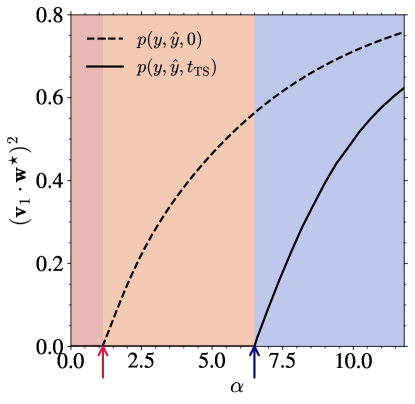
Figure 4: Evolution of the predicted squared overlap computed from Eq. 10 between the eigenvector associated to the smallest eigenvalue and the signal, namely $(\bm{v}_{1}\cdot\bm{w}^{\star})^{2}$. Two relevant times of the dynamics are shown: at initialization (dashed line) and on threshold states (solid line). The red (resp. blue) arrow indicates $\alpha_{\mathrm{BBP}}^{\mathrm{init}}=1.13$ (resp. $\alpha_{\mathrm{BBP}}^{\mathrm{TS}}=6.55$). The background colors refer to the three different regimes described in the left panel of Fig. 1.

3.2 BBP transition at initialization

In the setup described in the introduction, and before operating the gradient descent, $p(y,\hat{y},0)$ is the product of two Gaussian distributions. The aforementioned equations characterizing the BBP transition can therefore be solved to obtain the value $\alpha_{\mathrm{BBP}}^{\mathrm{init}}=1.13$ for the considered loss function $\ell_{a=1}$. As a consequence, whenever $\alpha>\alpha_{\mathrm{BBP}}^{\mathrm{init}}$, any initial condition $\bm{w}^{(0)}$ is characterized by a Hessian spectrum with an isolated left-most eigenvalue and an eigenvector $\bm{v}_{1}$ pointing towards the signal. More precisely, it has a finite overlap with the signal that grows with the value of $\alpha$ and which can be computed analytically from Eq. 10 (see the dashed line in Fig. 4).

3.3 BBP transition on threshold states

The characterization of $p(y,\hat{y},t_{\mathrm{TS}})$ is more involved than at initialization (note that $t_{\mathrm{TS}}=\infty$ for $N=\infty$). Indeed, right after a single step of gradient descent, $y$ and $\hat{y}$ are correlated. To pursue our analysis, we employ two methods allowing to approximate this joint distribution: (i) through adapted numerical simulations (described more precisely in Sect. 4) allowing to sample the threshold states. One can then evaluate empirically the expectations of Eqs. (8) and (9); (ii) through the statistical physics of disordered systems and the replica method (see Appendix B), as performed in [18, 31]. Those two methods grant us two consistent but different values of the BBP transition on threshold states that are respectively $\alpha_{\mathrm{BBP}}^{\mathrm{TS}}=6.55$ and $\alpha_{\mathrm{BBP}}^{\mathrm{1RSB,TS}}=6.9$. We expect the gap between these two to vanish when moving to more accurate RSB schemes and we adopt $\alpha_{\mathrm{BBP}}^{\mathrm{TS}}$ as the BBP threshold for the rest of the paper. In a similar way to initial states, for $\alpha>\alpha_{\mathrm{BBP}}^{\mathrm{TS}}$, the threshold states develop a negative direction and therefore turn from minima to saddles pointing towards $\pm\bm{w}^{\star}$ with an overlap shown as the solid line in Fig. 4.

3.4 Dynamics and dynamical BBP transitions

Comparing the results from $t=0$ and $t=t_{\mathrm{TS}}$ in Fig. 4, we find that gradient descent transports the initial state towards a location that is in an even rougher part of the landscape, and that does not allow recovery. For a given $\alpha$ such that $\alpha_{\mathrm{BBP}}^{\mathrm{init}}<\alpha<\alpha_{\mathrm{BBP}}^{\mathrm{TS}}$ and at a finite time $t_{\mathrm{BBP}}(\alpha)$, a BBP transition takes place during the descent as the informative isolated eigenvalue enters the bulk distribution (see Appendix C). The two ideal limits discussed above corresponds to $t_{\mathrm{BBP}}(\alpha_{\mathrm{BBP}}^{\mathrm{init}})=0$ and $t_{\mathrm{BBP}}(\alpha_{\mathrm{BBP}}^{\mathrm{TS}})=\infty$. In this regime, at finite $N$, the initial projection at $t=0$ in the downward direction towards the signal is of order $1/\sqrt{N}$. The component along this direction is therefore expected to grow exponentially (due to the negative curvature) but with a prefactor $1/\sqrt{N}$. In consequence, a time of order $\log N$ is needed to acquire a component of order one in this direction, and hence in the direction of the signal. For $N\rightarrow\infty$, and $\alpha_{\mathrm{BBP}}^{\mathrm{init}}<\alpha<\alpha_{\mathrm{BBP}}^{\mathrm{TS}}$, this time diverges, and the system looses the negative local curvature before actually being able to use it. However, this happens only in the strict large $N$ limit. Since this is a logarithmic effect in $N$, we expect the system to acquire a component of order one in the direction of the signal on moderate timescales and below $\alpha_{\mathrm{BBP}}^{\mathrm{TS}}$, even for very large $N$.
Once the system moves away from the equator, the loss landscape is expected to become more benign [44], therefore allowing for strong recovery. This phenomenon, which is expected to play a crucial role in practice, is already hinted in the inset of Fig. 2 where $m(t)$ grows on the loss plateau, therefore enabling the recovery at $\alpha<\alpha_{\mathrm{BBP}}^{\mathrm{TS}}$. We further test it by numerical experiments in the following.

4 Numerical analysis of the gradient descent dynamics

In this section, we run multiple experiments to analyze the behavior of gradient descent initialized both randomly and spectrally at finite values of $N$. To do so, we solve Eqs. (1) and (2) at fixed learning rate $\eta=6\times 10^{-3}$ for $T=9000\log_{2}(N)$ steps starting from different states depending on the initialization scheme. We also consider a system to perform strong recovery (or generalize well) whenever $\hat{\bm{w}}^{(T)}\cdot\bm{w}^{\star}/N\geq 0.99$.

Let us focus first on randomly initialized weights $\bm{w}^{(0)}\sim\mathcal{N}(\bm{0}_{N},\bm{I}_{N})$, leading to the strong recovery rates shown as solid lines in Fig. 5 for $N\in\{512,1024,2048\}$. We observe, in agreement with the previous arguments, that the simulations achieve strong recovery well before $\alpha_{\mathrm{BBP}}^{\mathrm{TS}}$ without clearly intersecting each other. This gap between the simulations and the BBP prediction was also observed in [31]. As discussed in the previous section, it is due to the displacement of the effective transition logarithmically with $N$ (see Appendix C). This shift is itself due to the initial local curvature and small but finite overlap $m(0)$ of the initial condition $\hat{\bm{w}}^{(0)}$ with the signal at finite $N$. In what follows, we devise more elaborated ways of exploring the landscape to bypass this effect.

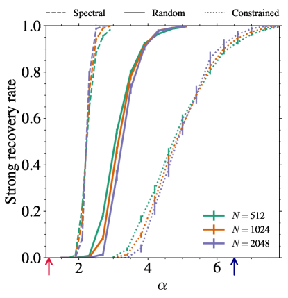
Figure 5: Strong recover rates as a function of $\alpha$ for several values of $N$ and different types of simulations: spectral, random, or constrained initializations. The red (resp. blue) arrow indicates $\alpha_{\mathrm{BBP}}^{\mathrm{init}}=1.13$ (resp. $\alpha_{\mathrm{BBP}}^{\mathrm{TS}}=6.55$). The error bars represent $95\%$ confidence intervals on the average.

4.1 A constrained optimization to probe threshold states

Efficiently sampling the threshold states numerically at finite $N$ is a critical aspect of our numerical analysis to show that:

1. These states exist in the phase retrieval loss landscape,

2. Gradient descent initialized randomly can find them,

3. They shift the BBP transition towards a larger value of $\alpha$, closer to the $N\to\infty$ prediction.

In order to sample the threshold states we propose a two-step procedure in which the estimate $\hat{\bm{w}}^{(t)}$ is first enforced to remain at the equator, and then free the optimization from the constraint to let the estimate evolve as described by Eq. (1). During this first step, we project the estimate at each time step $t$ in the subspace orthogonal to $\bm{w}^{\star}$ as

$$\hat{\bm{w}}^{(t+1)}_{\perp}=\left(\bm{I}_{N}-{\bm{w}^{\star}}^{\mkern-1.5mu\mathsf{T}}\bm{w}^{\star}\right)\hat{\bm{w}}^{(t+1)},$$ (11)

where $\hat{\bm{w}}^{(t+1)}$ is defined in Eq. (1). While sticking to the equator, the loss is still gradually decreased until it reaches a plateau, similarly to the inset of Fig. (2), but now with an enforced overlap of zero. In practice, we perform $t_{\mathrm{c}}=60000$ gradient descent steps with the constraint and converge to a state $\hat{\bm{w}}^{(t_{\mathrm{c}})}$ that we use as initialization for the standard gradient descent in a procedure called constrained initialization. Note however that this numerical scheme is not properly speaking sampling the threshold states since the gradient cannot be zero in the direction of the signal (its component is however $\sqrt{N}$ smaller than the gradient norm). We have checked numerically that the states we visit have the expected properties (marginal Hessian, BBP transition at the right $\alpha$, and eigenvalues behave as expected from Sect. 3).

One can appreciate the strong recovery rates obtained with gradient descent when using the constrained initialization as the dotted lines in Fig. 5. Contrary to what we observed in the case of random initializations, the successes for different values of $N$ now seem to converge at around $\alpha_{\mathrm{cons.}}^{\mathrm{SR}}\approx 5.5$. While this value is still not matching perfectly with the prediction $\alpha_{\mathrm{BBP}}^{\mathrm{TS}}=6.55$, it is much closer than what is observed in the random case. This means in particular that gradient descent is able to reach states that have less correlation with the signal than at initialization, making it harder to converge to a well-generalizing minimum, as predicted from the theory of Fig. 4. We leave to future works to solve the numerical discrepancy found above, which could be due to additional strong finite size effects.

4.2 Spectral initialization, weak recovery and loss landscape away from the equator

As stated in Sect. 3, when $\alpha>\alpha_{\mathrm{BBP}}^{\mathrm{init}}$, the Hessian matrix of any random configuration $\hat{\bm{w}}^{(0)}$ has a direction of least stability $\bm{v}_{1}$ displaying a non-zero overlap with the signal. This idea is at the heart of what is called spectral initialization proposed and studied in many previous works [14, 52, 25, 39]. By initializing the descent at $\hat{\bm{w}}^{(0)}=\bm{v}_{1}$, hence away from the equator where the landscape is less rough, one expects the system to avoid the bad minima, or at least to reach threshold states of larger latitudes that may exhibit a BBP transition at a smaller $\alpha$. From the perspective discussed in the previous sections, initializing along $\bm{v}_{1}$ is like taking advantage of the negative local curvature from the very beginning. The dashed lines of Fig. 5 support numerically these intuitions with a strong recovery transition occurring around $\alpha^{\mathrm{SR}}_{\mathrm{spec.}}\approx 2.14<\alpha^{\mathrm{SR}}_{\mathrm{random}}$. This is also emphasized by Fig. 6 in which we plot the evolution of the averaged overlaps both at initialization (crosses) and after $T$ steps of gradient descent (dots and solid lines).

There are several important findings associated to Fig. 6. First, there is a regime $\alpha_{\mathrm{BBP}}^{\mathrm{init}}<\alpha<\alpha^{\mathrm{SR}}_{\mathrm{spec.}}$ in which Hessian initialization leads to weak recovery, and a regime $\alpha>\alpha^{\mathrm{SR}}_{\mathrm{spec.}}$ in which it leads to strong recovery. This hints at a complex characterization of the loss landscape away from the equator, with minima still trapping the dynamics at low $\alpha$ but having a finite overlap with the signal, see [37] for related results and [44] for a Kac-Rice perspective on simpler models. Second, the spectral initialization shows that indeed by using the initial local negative curvature the system can achieve strong recovery well below $\alpha_{\mathrm{BBP}}^{\mathrm{TS}}$. Third, these results highlight the importance of a good initialization for gradient descent dynamics, especially in regimes as the ones found here in which the landscape is more benign at the beginning of the dynamics than later on.

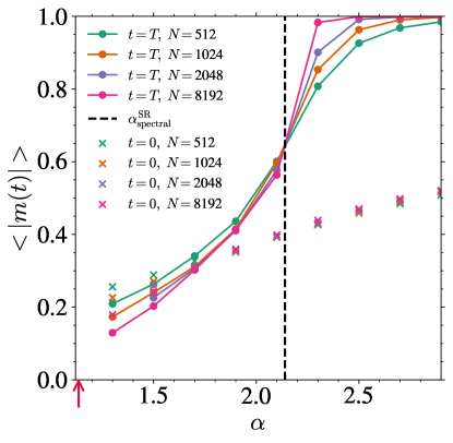
Figure 6: Evolution of the averaged overlap $\langle|m(t)|\rangle$ with $\alpha$ for several values of $N$ at times $0$ and $T$ using spectral initialization along $\bm{v}_{1}$. The red arrow denotes $\alpha_{\mathrm{BBP}}^{\mathrm{init}}$ and the vertical dashed black line corresponds to the strong recovery threshold $\alpha_{\mathrm{spec.}}^{\mathrm{SR}}$.

5 Discussion and perspectives

We provide in this paper a theoretical study analyzing the behavior of gradient descent in a high-dimensional and non-convex landscape through the noiseless phase retrieval problem with Gaussian measurements and in a teacher-student setup. Based on the analytical description of the Hessian at different relevant times of the gradient descent dynamics, i.e. on the initial and threshold states, we are able to understand the main condition of success and failure of gradient descent in the high-dimensional limit $N,M\to\infty$ with respect to $\alpha=M/N\sim O(1)$. From this analysis, we draw several conclusions and perspectives for phase retrieval.

The local landscape is more benign and informative at the beginning of the dynamics.

The value of $\alpha$ required to induce a BBP transition of the Hessian matrix towards the signal is larger on threshold states than at initialization. However, for very large $N$, although there exists one descending direction going towards $\pm\bm{w}^{\star}$ at $t=0$, gradient descent ignores it and is trapped by the threshold states when $\alpha\in\left[\alpha_{\mathrm{BBP}}^{\mathrm{init}},\alpha_{\mathrm{BBP}}^{\mathrm{TS}}\right]$. A much larger signal-to-noise ratio is required to render the latter unstable.

Finite $N$ random initializations benefit from this phenomenon.

Due to the BBP transition at initialization occurring at $\alpha_{\mathrm{BBP}}^{t=0}=1.13<\alpha_{\mathrm{BBP}}^{\mathrm{TS}}$, and to the finite value of $N$ used in practice, the overlap $m(t)$ between the estimate and the signal is able to grow during the descent. This enables the system to escape the equator on a timescale of order $\log N$ by leaving the rough part of the landscape and join benign regions. This is the mechanism that allows for successful optimization in practice, well before the algorithmic threshold corresponding to the high-dimensional limit $N\to\infty$ (the effect being logarithmic in $N$).

The importance of spectral initializations.

Given that the landscape is more benign at the beginning of the dynamics, spectral initializations can be very useful to escape from the equator before reaching the bad region. This phenomenon provides a showcase for a strong advantage of spectral initializations and, more generally, of spectral properties to improve optimization in non convex high-dimensional landscape – a research axis that received a lot of attention recently in the context of deep learning [20, 48, 54].
Our theoretical analysis of the BBP transitions holds at the equator, where $m=0$. To get a better understanding of spectral initializations, one must study the topological properties of the landscape as a function of both $\alpha$ and $m$. This could be done using the Kac-Rice method for loss functions in the form of Eq. (3) as proposed in [28].

The values of $\alpha$ at which the dynamical BBP transitions occur depend strongly on the choice of the loss function. Thus, it would be interesting to find losses that enhance this phenomenon and lead to an earlier signal recovery, as done in [39] for spectral initializations and in [11, 13] for landscape trivialization. Finally, it would be worth characterizing this phenomenon for a broader class of loss functions. We show a first case study by varying $a$ in Eq. (3) (see Appendix D).

Acknowledgments

The authors thank Stefano Sarao Mannelli for sharing his code used in [31]. T.B. further thanks Aurélien Decelle and Bruno Loureiro for useful discussions on the topic. G.B. acknowledges support from the French government under the management of the Agence Nationale de la Recherche as part of the “Investissements d’avenir” program, reference ANR-19-P3IA0001 (PRAIRIE 3IA Institute). C.C. acknowledges financial support from PNRR MUR project PE0000013-FAIR and from MUR through PRIN2022 project 202234LKBW-Land(e)scapes.

Appendix A Random matrix analysis of the Hessian

A.1 Characterizing the eigenspectrum bulk

Omitting the spherical constraint – which is just a translation of the eigensupport – the Hessian matrix can be written as a sum of $M$ free matrices (when ignoring the potential outlier eigenvalue),

$$\mathcal{H}(\bm{w})=\sum_{i=1}^{M}\bm{X}^{(i)},$$ (12)

with $\bm{X}^{(i)}=f_{i}\bm{x}_{i}\bm{x}_{i}^{\mkern-1.5mu\mathsf{T}}$. To evaluate the limiting Stieltjes transform of $\mathcal{H}$, denoted $\mathcal{S}_{\mathcal{H}}$, we use the properties of the R-transform for free random matrices

$$R_{\mathcal{H}}=\sum_{i=1}^{M}R^{(i)},$$ (13)

with $R^{(i)}$ the R-transform of $\bm{X}^{(i)}$ which is given by

$$\mathcal{S}^{(i)}(z)=\frac{1}{N}\sum_{i=1}^{N}\frac{1}{z-\gamma_{i}},$$ (14)

where $\gamma_{i}$ are the eigenvalues of $\bm{X}^{(i)}$. Since it is a rank-one matrix, its eigenvalues are $0$ with multiplicity $N-1$ and $f_{i}$ with multiplicity one, leading to

$$\mathcal{S}^{(i)}(z) =\frac{1}{z}-\frac{1}{Nz}+\frac{1}{N\left(z-f_{i}\right)}.$$ (15)

We now need to reverse this relation to obtain $z$ as a function of $\mathcal{S}$. In the large $N$ limit, $\mathcal{S}^{(i)}(z)=1/z$ and we use this to reverse the relation in the high-dimensional limit as

$$z =\frac{1}{\mathcal{S}^{(i)}\left(1+\frac{1}{N}\left[1-\frac{1}{1-f_{i}\mathcal{S}^{(i)}}\right]\right)}.$$ (16)

At first order in $1/N$, we can hence write

$$z =\frac{1}{\mathcal{S}^{(i)}}+\frac{1}{N}\left[\frac{f_{i}}{1-f_{i}\mathcal{S}^{(i)}}\right]+O\left(\frac{1}{N}\right).$$ (17)

The R-transform of $\bm{X}^{(i)}$ is therefore

$$R^{(i)}=\frac{1}{N}\left[\frac{f_{i}}{1-f_{i}\mathcal{S}^{(i)}}\right].$$ (18)

When $N\to\infty$, the R-transform is expected to concentrate around its mean and we obtain

$$R_{\mathcal{H}}\underset{N\rightarrow\infty}{\rightarrow}\alpha\mathbb{E}_{y,\hat{y}}\left[\frac{f}{1-f\mathcal{S}_{\mathcal{H}}(z)}\right].$$ (19)

This finally leads to the self-consistent equation given in the main text Eq. (5)

$$\mathcal{S}_{\mathcal{H}}(z)^{-1}=z-\alpha\mathbb{E}_{y,\hat{y}}\left[\frac{f}{1-f\mathcal{S}_{\mathcal{H}}(z)}\right],$$ (20)

that fully characterizes the bulk of the eigenspectrum through the Sokhotski–Plemelj formula.

The left edge of the bulk $\lambda_{-}$ can be found through the maximum of $z(\mathcal{S})$, satisfying

$$\frac{\partial z(\mathcal{S})}{\partial\mathcal{S}}_{\rvert_{\mathcal{S}=\mathcal{S}_{-}}}=0.$$ (21)

Since $z(\mathcal{S})=R_{\mathcal{H}}(\mathcal{S})+1/\mathcal{S}$, we find that

$$\mathcal{S}_{-}=\left(\mathbb{E}_{y,\hat{y}}\left[\frac{\alpha^{2}f^{2}}{\left(1-f\mathcal{S}_{-}\right)^{2}}\right]\right)^{-1/2},$$ (22)

which is the left-edge condition given in Eq. (9).

A.2 Derivation of the overlap

To compute the squared overlap, let us first remark that the problem is invariant by rotation, hence we can focus only on computing the first component of the Stieltjes transform and we can decompose $\mathcal{S}_{11}(z)$ using the eigenvector $\bm{v}_{i}$ of $\mathcal{H}$ as

$$\mathcal{S}_{11}(z)=\sum_{i=1}^{N}\frac{|\left[\bm{v}_{i}\right]_{1}|^{2}}{z-\lambda_{i}}.$$ (23)

Noting $\bm{v}_{1}$ the eigenvector associated to the outlier eigenvalue $\lambda_{\star}$, we have

$$\lim_{z\rightarrow\lambda_{\star}}\mathcal{S}_{11}(z)=\frac{\left(\bm{v}_{1}^{\mkern-1.5mu\mathsf{T}}\bm{w}_{\star}\right)^{2}}{z-\lambda_{\star}}.$$ (24)

By l’Hospital’s rule,

$$\left(\bm{v}_{1}^{\mkern-1.5mu\mathsf{T}}\bm{w}_{\star}\right)^{2}=\lim_{z\rightarrow\lambda_{\star}}\frac{z-\lambda_{\star}}{z-\Sigma(z)}=\frac{1}{1-\partial_{z}\Sigma(z)_{|z=\lambda_{\star}}},$$ (25)

where $\Sigma(z)$ is given in Eq. (7).

Appendix B Replica method for the computation of $p(y,\hat{y},t_{\mathrm{TS}})$

Let us first write the Boltzmann distribution associated to the system as

$$P(\bm{w})=\frac{1}{Z(\beta)}\exp{-\beta\mathcal{L}(\bm{w})},$$ (26)

where $Z(\beta)$ is the partition function and $\mathcal{L}(\bm{w})$ is the energy or cost function. The corresponding free energy per particle is

$$\phi(\beta)=-\frac{1}{N\beta}\log Z(\beta),$$ (27)

which is tightly coupled with some interesting macroscopic quantities of the system, like the average loss function, the expected overlap, but also to the joint probability distribution $p(y,\hat{y})$ of true and estimated labels. As first explained in [18] and also exploited in [33], the typical distribution is given by $p(y,\hat{y})=\mathbb{E}_{\bm{w}}\left[\overline{\hat{p}(y,\hat{y})}\right]$, where $\hat{p}$ denotes the empirical measure, the overline is the average over the disorder (here the dataset $\{\bm{x}_{i}\}_{m=1}^{M}$), and the expectation is taken over the Boltzmann measure. The partition function can be written in terms of $\hat{p}(y,\hat{y})$ as

$$\overline{Z(\beta)} =\overline{\int_{\mathbb{S}^{N-1}}\differential\bm{w}\exp{-\beta\mathcal{L}(\bm{w})}},$$ (28)

$$=\overline{\int_{\mathbb{S}^{N-1}}\differential\bm{w}\exp{-\frac{\beta}{2}\sum_{i=1}^{M}\ell(y_{i},\hat{y}_{i})}},$$ (29)

$$=\overline{\int_{\mathbb{S}^{N-1}}\differential\bm{w}\exp{-\frac{\beta M}{2}\int\differential y\differential\hat{y}\ell(y,\hat{y})\hat{p}(y,\hat{y})}},$$ (30)

for a loss function of the form Eq. (2).

From this last expression, the distribution $p(y,\hat{y})$ is accessible through the functional derivative of the free energy as

$$\frac{\delta\overline{\phi}}{\delta\ell(y,\hat{y})}=-\frac{1}{N\beta}\frac{\delta\overline{\log Z(\beta)}}{\delta\ell(y,\hat{y})}=\frac{\alpha}{2}\mathbb{E}_{\bm{w}}\left[\overline{\hat{p}(y,\hat{y})}\right]=\frac{\alpha}{2}p(y,\hat{y}).$$ (31)

This gives us some motivation for the computation of the log partition function, and more precisely its first moment if we can expect large deviation principle to apply to obtain the ”typical” behavior of the system.

B.1 Replicated partition function

To compute the average free energy per particle, we can use the replica method stating that

$$\overline{\log Z}=\lim_{n\rightarrow 0}\frac{\overline{Z^{n}}-1}{n}.$$ (32)

In practice, we will compute $\overline{Z^{n}}$ for $n\in\mathbb{N}$ and then analytically continue it to $n\in\mathbb{R}$ in order to finally take the $n\rightarrow 0$ limit. The problem now boils down to compute $\overline{Z^{n}}$ which can be expressed as the partition function associated to the product of $n$ independent systems with the partition function $Z(\beta)$ and gives

$$Z(\beta)^{n}=\int_{\mathbb{S}^{N-1}}\prod_{a=1}^{n}\left[\differential\bm{w}\exp{-\beta\sum_{m=1}^{M}\ell\left(\bm{x}_{m}\cdot\bm{w}^{\star},\bm{x}_{m}\cdot\bm{w}\right)}\right].$$ (33)

Let us introduce $r_{m}^{(a)}=\bm{x}_{i}\cdot\bm{w}^{(a)}$, the overlap between the entries and the state of the $a$^th system, reserving the index zero for the overlap with the ground truth, meaning with $r_{m}^{(0)}=\bm{x}_{i}^{\mkern-1.5mu\mathsf{T}}\bm{w}^{\star}$. These new variables are introduced through delta functions that we replace by their Fourier representation. We therefore get

$$Z(\beta)^{n}\propto\int_{\mathbb{S}^{N-1}}\prod_{a=1}^{n}\differential\bm{w}^{(a)}\int\prod_{a=0}^{n}\prod_{m=1}^{M}\differential r_{m}^{(a)}\int\prod_{a=0}^{n}\prod_{m=1}^{M}\differential\hat{r}_{m}^{(a)}\\ \exp{-\beta\sum_{a=1}^{n}\sum_{m=1}^{M}\ell\left(r_{m}^{(0)},r_{m}^{(a)}\right)+i\sum_{a=0}^{n}\sum_{m=1}^{M}\hat{r}_{m}^{(a)}r_{m}^{(a)}+i\sum_{a=0}^{n}\sum_{m=1}^{M}\hat{r}_{m}^{(a)}\bm{x}_{i}\cdot\bm{w}^{(a)}}.$$ (34)

This allows us to compute the expectation over the disorder since, now, it only acts on the last term in the exponential. This integral can be evaluated using the Hubbard-Stratonovich identity as

$$E(X) =\mathbb{E}_{\bm{X}}\left[\exp{i\sum_{a=0}^{n}\sum_{m=1}^{M}\hat{r}_{m}^{(a)}\bm{x}_{i}\cdot\bm{w}^{(a)}}\right],$$ (35)

$$\propto\exp{-\frac{1}{2N}\sum_{a,b=0}^{n}\sum_{m=1}^{M}\hat{r}_{m}^{(a)}\hat{r}_{m}^{(b)}\bm{w}^{(a)}\cdot\bm{w}^{(b)}}.$$ (36)

Let us now consider the overlap between two replicas, $q_{ab}=\frac{1}{N}\bm{w}^{(a)}\cdot\bm{w}^{(b)}$. Similar to previously, we use the index zero for the overlap with the signal $\bm{w}^{\star}$ such that $\forall a\in\left[1,n\right],q_{0a}=m$ and we also have $\forall a\in\left[0,n\right],q_{aa}=1$. All these overlaps are regrouped in an $(n+1)\times(n+1)$ matrix $\bm{Q}$ and are introduced through a delta function again. It then reads

$$\overline{Z(\beta)^{n}}\propto\int\prod_{0\leq a\leq b\leq n}\differential q_{ab}\int\prod_{a=0}^{n}\prod_{m=1}^{M}\differential r_{m}^{(a)}\int\prod_{a=0}^{n}\prod_{m=1}^{M}\differential\hat{r}_{m}^{(a)}\underbrace{\int_{\mathbb{S}^{N-1}}\prod_{a=1}^{n}\differential\bm{w}^{(a)}\prod_{0\leq a\leq b\leq n}\delta(Nq_{ab}-\bm{w}^{(a)}\cdot\bm{w}^{(b)})}_{J(\bm{Q})}\\ \exp{-\beta\sum_{a=1}^{n}\sum_{m=1}^{M}\ell\left(r_{m}^{(0)},r_{m}^{(a)}\right)+i\sum_{a=0}^{n}\sum_{m=1}^{M}\hat{r}_{m}^{(a)}r_{m}^{(a)}-\frac{1}{2}\sum_{a,b=0}^{n}\sum_{m=1}^{M}\hat{r}_{m}^{(a)}\hat{r}_{m}^{(b)}q_{ab}},$$ (37)

with $J(\bm{Q})=|\bm{Q}|^{N/2}$ in the large $N$ limit [55], consequently giving, after factorizing the $M$ integrals

$$\overline{Z(\beta)^{n}}\propto\int\prod_{0\leq a\leq b\leq n}\differential q_{ab}\exp{\frac{N}{2}\log|\bm{Q}|}\Bigg{[}\int\prod_{a=0}^{n}\differential r^{(a)}\int\prod_{a=0}^{n}\differential\hat{r}^{(a)}\\ \exp{-\beta\sum_{a=1}^{n}\ell\left(r^{(0)},r^{(a)}\right)+i\sum_{a=0}^{n}\hat{r}^{(a)}r^{(a)}-\frac{1}{2}\sum_{a,b=0}^{n}\hat{r}^{(a)}\hat{r}^{(b)}q_{ab}}\Bigg{]}^{M}.$$ (38)

Performing the integral over $\hat{r}$ using the Hubbard-Stratonovich identity again and setting $N\to\infty$, we finally obtain the replicated partition function

$$\overline{Z(\beta)^{n}}\propto\exp{N\operatorname*{extr}_{\bm{Q}}S(\bm{Q})},$$ (39)

with

$$S(\bm{Q}) =\frac{1}{2}\log|\bm{Q}|+\alpha\log\int\prod_{a=0}^{n}\frac{\differential r^{(a)}}{\left(2\pi\right)^{n/2}\sqrt{|\bm{Q}|}}\exp{-\beta\sum_{a=1}^{n}\ell\left(r^{(0)},r^{(a)}\right)-\frac{1}{2}\sum_{a,b}r^{(a)}\bm{Q}^{-1}_{ab}r^{(b)}},$$ (40)

$$=S_{1}+S_{2}$$ (41)

where $S_{1}$ is an entropic factor counting the number of spherical couplings that satisfies the constraints $q_{ab}=\bm{w}^{(a)}\cdot\bm{w}^{(a)}/N$ and $S_{2}$ is the energetic contribution specific to the learning rule in which appears the energy function.

B.2 One-step replica symmetry breaking (1RSB)

Notice that we turned the initial problem of computing a high-dimensional integral into a high-dimensional optimization over $(n+1)^{2}$ variables in Eq. (40). Although this may seem doomed, we can purse our analytical treatment by using an ansatz on the form of $\bm{Q}$. The simplest form of hypothesis is replica symmetry assuming $q_{ab}=q_{0}$ everywhere. However, this assumption breaks in the regime we are in and one needs to break the symmetry. In our case, we use the first level of symmetry breaking (1RSB) assuming

$$\bm{Q}_{\mathrm{1RSB}}=\left(\begin{array}[]{ c | c c c c c c }1&\lx@intercol\hfil m\hfil\lx@intercol&\lx@intercol\hfil\cdots\hfil\lx@intercol&\lx@intercol\hfil m\hfil\lx@intercol\\ \cline{1-7}\cr&\lx@intercol\hfil\raisebox{7.20007pt}[0.0pt][0.0pt]{}\hfil\lx@intercol\vrule\lx@intercol&q_{0}&q_{0}&q_{0}&q_{0}\\ \raisebox{7.20007pt}[0.0pt][0.0pt]{$m$}&\lx@intercol\hfil\raisebox{7.20007pt}[0.0pt][0.0pt]{$\tilde{\bm{Q}}$}\hfil\lx@intercol\vrule\lx@intercol&q_{0}&q_{0}&q_{0}&q_{0}\\ \cline{2-5}\cr&q_{0}&q_{0}&\vrule\lx@intercol\hfil\hfil\lx@intercol&\lx@intercol\hfil\hfil\lx@intercol\vrule\lx@intercol&q_{0}&q_{0}\\ \raisebox{7.20007pt}[0.0pt][0.0pt]{$\vdots$}&q_{0}&q_{0}&\vrule\lx@intercol\hfil\raisebox{7.20007pt}[0.0pt][0.0pt]{$\tilde{\bm{Q}}$}\hfil\lx@intercol\vrule\lx@intercol&q_{0}&q_{0}\\ \cline{4-7}\cr&q_{0}&q_{0}&q_{0}&q_{0}&\vrule\lx@intercol\hfil\hfil\lx@intercol&\lx@intercol\hfil\hfil\lx@intercol\vrule\lx@intercol\\ \raisebox{7.20007pt}[0.0pt][0.0pt]{$m$}&q_{0}&q_{0}&q_{0}&q_{0}&\vrule\lx@intercol\hfil\raisebox{7.20007pt}[0.0pt][0.0pt]{$\tilde{\bm{Q}}$}\hfil\lx@intercol\vrule\lx@intercol\\ \cline{6-7}\cr\end{array}\hskip 1.42271pt\right)\in\mathbb{R}^{(n+1)\times(n+1)},$$ (42)

with $\tilde{\bm{Q}}$ a matrix of size $p\times p$ with one on the diagonal and $q_{1}$ everywhere else. Under this assumption, the action can be written in terms of the four parameters $n$, $m$, $p$, $q_{0}$ and $q_{1}$. This hence reduces the saddle point method to extremize over those parameters only in Eq. 39. This type of matrix was heavily studied in the statistical physics literature and one result of particular interest for us is to remark that $\bm{Q}_{\mathrm{1RSB}}$ has three eigenvalues $\tilde{\lambda}_{i}$ with multiplicities $d_{i}$ given by [15]

$$\begin{cases}\tilde{\lambda}_{1}=1-q_{1},&d_{1}=n\left(1-\frac{1}{p}\right),\\ \tilde{\lambda}_{2}=p(q_{1}-q_{0})+(1-q_{1}),&d_{2}=\frac{n}{p}-1,\\ \tilde{\lambda}_{3}=p(q_{1}-q_{0})+(1-q_{1})+n(q_{0}-m^{2}),&d_{3}=1.\\ \end{cases}\,$$ (43)

Using these eigenvalues, we can evaluate the entropy in the action as

$$S_{1}^{\mathrm{1RSB}}(q_{0},q_{1},m,p)=\frac{n}{2}\left[\log(1-q_{1})+\frac{1}{p}\log\frac{1-q_{1}+p(q_{1}-q_{0})}{1-q_{1}}+\frac{q_{0}-m^{2}}{1-q_{1}+p(q_{1}-q_{0})}\right]+O(n^{2}).$$ (44)

For the energetic term, one has to use the form of $\bm{Q}_{\mathrm{1RSB}}$ to work out that

$$-\frac{1}{2}\sum_{a,b}\hat{r}^{(a)}\hat{r}^{(b)}q_{ab}=-\frac{1}{2}\Bigg{[}\hat{r}^{(0)}\hat{r}^{(0)}+(1-q_{1})\sum_{a=1}^{n}\hat{r}^{(a)}\hat{r}^{(a)}\\ +(q_{1}-q_{0})\sum_{P_{a}=1}^{n/p}\left(\sum_{a\in P_{a}}\hat{r}^{(a)}\right)^{2}+q_{0}\left(\sum_{a=1}^{n}\hat{r}^{(a)}\right)^{2}+2m\sum_{a=1}^{n}r^{(a)}r^{(0)}\Bigg{]}.$$ (45)

Substuting it into $S_{2}$ gives

$$S_{2}^{\mathrm{1RSB}}(q_{0},q_{1},m,p)\underset{n\rightarrow 0^{+}}{\approx}\frac{\alpha n}{p}\int\differential\eta\int\differential r^{(0)}D(r^{(0)},\eta)\log\Bigg(\int\frac{\differential\eta_{P}}{\sqrt{2\pi(q_{1}-q_{0})}}\exp{-\frac{\eta_{P}^{2}}{2(q_{1}-q_{0})}}{\\ }\left[\int\frac{\differential r}{\sqrt{2\pi}}\exp{-\beta\Psi(r^{(0)},r,\eta_{P},\eta,q_{1})}\right]^{p}\Bigg{missing}),$$ (46)

where

$$\Psi(r^{(0)},r,\eta_{P},\eta,q_{1})=\ell(r^{(0)},r)+\frac{(\eta_{P}+\eta-r)^{2}}{2\beta(1-q_{1})}.$$ (47)

B.3 Zero-temperature limit and free energy

The 1RSB free energy is defined as the zero temperature limit ($\beta\to\infty$) of the extremum of the 1RSB action $S^{\mathrm{1RSB}}=S(\bm{Q}_{\mathrm{1RSB}})$

$$\phi_{\mathrm{1RSB}} =\lim_{\beta\rightarrow+\infty}\lim_{n\rightarrow 0^{+}}-\frac{1}{n\beta}S_{1}^{\mathrm{1RSB}}(q_{0},q_{1},m,p)-\frac{1}{n\beta}S_{2}^{\mathrm{1RSB}}(q_{0},q_{1},m,p).$$ (48)

While taking the $\beta\rightarrow+\infty$ limit, we set $q_{1}\rightarrow 1$ keeping both $\chi=\beta(1-q_{1})$ and $z=\beta p$ of order one. Putting it all together, and setting $m$ to zero by remarking it satisfies the saddle-point $\partial_{m}S^{\mathrm{1RSB}}=0$, we end up with the 1RSB free energy

$$\phi_{\mathrm{1RSB}}(\chi,z,q_{0})=-\frac{1}{2z}\log\frac{\chi+z(1-q_{0})}{\chi}-\frac{1}{2}\frac{q_{0}}{\chi+z(1-q_{0})}-\frac{\alpha}{z}\int\differential\eta\int\differential r^{(0)}D(r^{(0)},\eta)\\ \log\left(\int\frac{\differential\eta_{P}}{\sqrt{2\pi(1-q_{0})}}\exp{-\frac{\eta_{P}^{2}}{2(1-q_{0})}-z\Psi_{0}(r^{(0)},\eta_{P},\eta,\chi)}\right),$$ (49)

with

$$\Psi_{0}(r^{(0)},\eta_{P},\eta,\chi) =\min_{\tilde{r}}\ell(r^{(0)},\tilde{r})+\frac{(\eta_{P}+\eta-\tilde{r})^{2}}{2\chi},$$ (50)

$$D(r^{(0)},\eta) =\frac{1}{2\pi\sqrt{q_{0}}}\exp{-\frac{{r^{(0)}}^{2}q_{0}\eta+\eta^{2}}{2q_{0}}}.$$ (51)

From Eq. (31), we need to take the functional derivative of the free energy with respect to the loss function $\ell(y,\hat{y})$ to obtain the joint distribution of true and estimated labels on threshold states $p(y,\hat{y},t_{\mathrm{TS}})$. This gives

$$p(y,\hat{y},t_{\mathrm{TS}})=\frac{1}{\sqrt{2\pi}}\int\frac{\differential\eta}{\sqrt{2\pi q_{0}}}\exp{-\frac{y^{2}q_{0}+\eta^{2}}{2q_{0}}}\frac{\exp{-\frac{\hat{y}^{2}}{2(1-q_{0})}-z\Psi_{0}(y,\hat{y},\eta,\chi)}}{\int\differential\tilde{y}\exp{-\frac{\tilde{y}^{2}}{2(1-q_{0})}-z\Psi_{0}(y,\tilde{y},\eta,\chi)}},$$ (52)

which is equivalent to the finding of [31] if we set $q_{0}=0$. Finally, the parameters $\chi$, $z$, and $q_{0}$ are fixed via the saddle-point equations obtained from $\partial_{\chi}S^{\mathrm{1RSB}}=0$ and $\partial_{q_{0}}S^{\mathrm{1RSB}}=0$, giving

$$\frac{1}{z}\left(\frac{1}{\chi}-\frac{1}{\chi+z(1-q_{0}))}\right)+\frac{q_{0}}{(\chi+z(1-q_{0}))^{2}}=\alpha\int\differential\eta\int\differential r^{(0)}D(r^{(0)},\eta)\\ \frac{\int\differential\eta_{P}\exp{-\frac{\eta_{P}^{2}}{2(1-q_{0})}-z\Psi_{0}(r^{(0)},\eta_{P},\eta,\chi)}\left(\partial_{\eta_{P}}\Psi_{0}(r^{(0)},\eta_{P},\eta,\chi)\right)^{2}}{\int\differential\eta_{P}\exp{-\frac{\eta_{P}^{2}}{2(1-q_{0})}-z\Psi_{0}(r^{(0)},\eta_{P},\eta,\chi)}},$$ (53)

$$-\frac{q_{0}}{(\chi+z(1-q_{0}))^{2}}=\frac{2\alpha}{z^{2}}\int\differential\eta\int\differential r^{(0)}D(r^{(0)},\eta)\frac{\eta^{2}-q_{0}}{2q_{0}^{2}}\\ \log\left(\int\frac{\differential\eta_{P}}{\sqrt{2\pi(1-q_{0})}}\exp{-\frac{\eta_{P}^{2}}{2(1-q_{0})}-z\Psi_{0}(r^{(0)},\eta_{P},\eta,\chi)}\right)+\frac{\alpha}{z^{2}(1-q_{0})}\\ -\frac{\alpha}{z^{2}(1-q_{0})^{2}}\int\differential\eta\int\differential r^{(0)}D(r^{(0)},\eta)\frac{\int\differential\eta_{P}\exp{-\frac{\eta_{P}^{2}}{2(1-q_{0})}-z\Psi_{0}(r^{(0)},\eta_{P},\eta,\chi)}\eta_{P}^{2}}{\int\differential\eta_{P}\exp{-\frac{\eta_{P}^{2}}{2(1-q_{0})}-z\Psi_{0}(r^{(0)},\eta_{P},\eta,\chi)}}.$$ (54)

On the other hand, $z$ is fixed by the marginality condition of the Hessian spectrum that we assume on threshold states [18, 31]. Using Eq. (52) in Eqs. (8) and (9) yields the value $\alpha_{\mathrm{BBP}}^{\mathrm{TS,1RSB}}=6.9$. We expect that breaking further the symmetry by assuming substructures in $\bm{Q}_{\mathrm{1RSB}}$ would reduce the gap with the $\alpha_{\mathrm{BBP}}^{\mathrm{TS}}=6.55$ obtained from the sampling of threshold states but leave this aspect for further investigations.

Appendix C Details of the numerical experiments

Effects of hyperparameters on the numerical results.

All the figures of the main text are obtained by fixing $\eta=6\times 10^{-3}$ and performing $t_{\mathrm{c}}=60\,000$ steps for the constrained initialization. Our analysis focuses on gradient flow with $\eta\to 0$. In practice, we set $\eta$ sufficiently small not to have any impact on the presented phenomena. The left panel of Fig. 7 illustrates for instance the strong recovery rates obtained when $\eta$ is decreased to $6\times 10^{-4}$ but keeping the total simulation time $\eta T$ constant (with $10t_{\mathrm{c}}$ steps for the constrained initialization). In this case, the dynamical transition is not displaced significantly and is found at around $\alpha\approx 5.65$, agreeing with the one in the main text under the error bars. In a similar way, we report in the right panel of Fig. 7 the strong recovery rates obtained by fixing $\eta$ to its fiducial value of $0.006$, $N=512$, and varying $t_{\mathrm{c}}$ from $15\,000$ to $120\,000$. The simulations share the same initializations. When $t_{\mathrm{c}}$ is above $30\,000$, we do not see any impact on the strong recovery rates, and hence on the dynamical transition. This shows the robustness of the numerical experiments with respect to those hyperparameters.

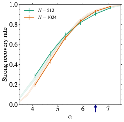
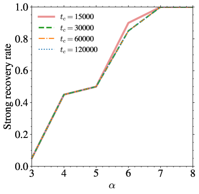
Figure 7: (Left) Effect of decreasing the learning rate by a factor ten ($\eta=6\times 10^{-4}$, solid lines) on the strong recovery rate of the constrained simulations. The shaded areas are the rates obtained with $\eta=6\times 10^{-3}$, the value used in the main text. The blue arrow indicates $\alpha_{\mathrm{BBP}}^{\mathrm{TS}}$ computed for $a=1$. (Right) Effect of varying $t_{\mathrm{c}}$, the number of steps to approach the threshold states in constrained initialization. When $t_{\mathrm{c}}>30\,000$, they all lead to the same strong recovery rates.

Logarithmic scaling of the strong recovery rates.

In Fig. 9 can be found some evidences of the displacement of the strong recovery rates obtained in Fig. 5 for randomly initialized weights. In this case, the effective transition is shown to increase with $\log N$, as a consequence of the local initial curvature coupled with the initial overlap $m(0)$ of order $1/\sqrt{N}$.

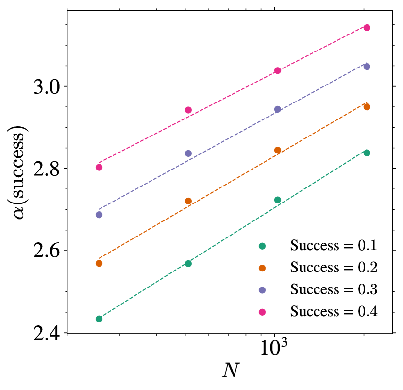
Figure 8: Scaling of $\alpha$ for several fixed strong recovery rates (shown in Fig. 5) for random initializations and $N\in\{256,512,1024,2048\}$.

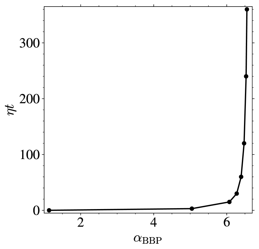
Figure 9: Evolution of the simulation time $\eta t$ at which a BBP transition takes place with $\alpha$ in simulations with constrained initializations. The timesteps run from zero to $t_{\mathrm{c}}=60\,000$.

Numerical estimate of the BBP transition on threshold states.

In Sect. 3 and Sect. 4, we use a numerical approach to extract $p(y,\hat{y},t_{\mathrm{TS}})$ and compute $\alpha_{\mathrm{BBP}}^{\mathrm{TS}}$. The method relies on sampling the threshold states using the constrained initialization (see Sect. 4.1) to then compute the expectations from Eqs. (8), (9), and  (10) by averaging numerically. Of course, this means that we are using finite $N$ simulations to compute expectations derived for $N\to\infty$. In practice, we use $N=\{512,1024,2048\}$ simulations to perform a finite-size scaling analysis of $\alpha_{\mathrm{BBP}}^{(t)}$. We checked that this procedure allows us to retrieve the analytical value of $\alpha_{\mathrm{BBP}}^{\mathrm{init}}=1.13$ with great accuracy and obtain on threshold states the value given in the main text of $\alpha_{\mathrm{BBP}}^{\mathrm{TS}}=6.55$. In order to check the consistency with larger values of $N$, we also compared this result with hundreds of numerical simulations with $N=8192$ leading to the same value.

Time evolution of the BBP transition.

It is possible to extend the approach described above to other times than the limits $t(\alpha_{\mathrm{BBP}}^{\mathrm{init}})=0$ and $t(\alpha_{\mathrm{BBP}}^{\mathrm{TS}})=\infty$ by computing averages over $p(y,\hat{y},t)$. This is shown in Fig. 9 with the evolution of the simulation time below which a BBP transition takes place with $\alpha$. After this time, the outlier eigenvalue enters the bulk. For intermediate values of $\alpha_{\mathrm{BBP}}^{\mathrm{init}}<\alpha<\alpha_{\mathrm{BBP}}^{\mathrm{TS}}$, the BBP transition occurs in finite times.

Appendix D Impact of the loss function on the BBP transitions

In the main text, we focused on the loss function $\ell_{a}(y,\hat{y})$ from Eq.(3) with $a=1$. The precise values of the BBP transitions however depend on the choice of $\ell$ and some other choice may lead to more favorable landscapes enabling earlier strong recovery. To illustrate this, we plot in the left panel of Fig. 10 the evolution of $\alpha_{\mathrm{BBP}}^{\mathrm{init}}$ computed for several values of $a$. Lowering $a$ leads to larger $\alpha_{\mathrm{BBP}}^{\mathrm{init}}$ meaning more samples are required to start having the local curvature towards the signal at initialization. Considering $a=0.1$, we find for instance $\alpha_{\mathrm{BBP}}^{\mathrm{init}}=2.16$ and $\alpha_{\mathrm{BBP}}^{\mathrm{TS}}=4.65$. Even though the initial states have a downward direction towards the signal at larger values of the signal-to-noise ratio than for $a=1$, threshold states on their side develop an instability earlier. This is clearly seen in right panel of Fig. 10 where the algorithmic transition occurs earlier than in Fig. 5 for both random and constrained initializations. In this case, we also report a logarithmic scaling of success rates with $N$ for random initializations while the curves intersect nicely with the constrained initializations at around $\alpha_{\mathrm{cons.}}\approx 4.5$. This value is also much closer to the $N\to\infty$ prediction than for $a=1$ used in the main text.

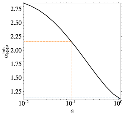
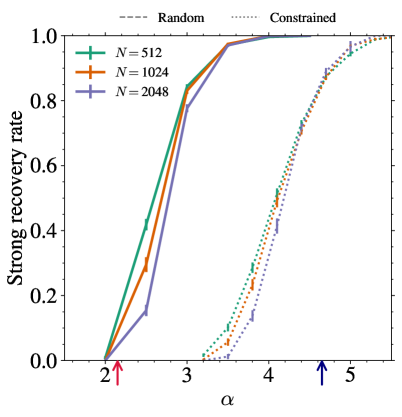
Figure 10: (Left) Evolution of $\alpha_{\mathrm{BBP}}^{\mathrm{init}}$ with $a$, the normalization of the loss function (3). The lower $\alpha_{\mathrm{BBP}}^{\mathrm{init}}$, the more favorable the landscape at initialization. The two colored dashed lines refer to the values of $a=1$ and $a=0.1$ discussed throughout the main text and in Appendix D respectively. (Right) Strong recovery rates for the case of a loss function $\ell_{a=0.1}$ with random and constrained initializations. The red (resp. blue) arrow indicates $\alpha_{\mathrm{BBP}}^{\mathrm{init}}=2.15$ (resp. $\alpha_{\mathrm{BBP}}^{\mathrm{TS}}=4.65$) computed in this case.

References

- Annesi et al. [2023] Annesi, B. L., Lauditi, C., Lucibello, C., Malatesta, E. M., Perugini, G., Pittorino, F., and Saglietti, L. Star-shaped space of solutions of the spherical negative perceptron. Phys. Rev. Lett., 131:227301, Nov 2023. doi: 10.1103/PhysRevLett.131.227301. URL https://link.aps.org/doi/10.1103/PhysRevLett.131.227301.
- Arnaboldi et al. [2023] Arnaboldi, L., Krzakala, F., Loureiro, B., and Stephan, L. Escaping mediocrity: how two-layer networks learn hard single-index models with sgd. 5 2023. URL http://arxiv.org/abs/2305.18502.
- Arous et al. [2021] Arous, G. B., Gheissari, R., Arous, B., and Gheissari, J. Online stochastic gradient descent on non-convex losses from high-dimensional inference, 2021.
- Baik et al. [2005] Baik, J., Arous, G. B., and Péché, S. Phase transition of the largest eigenvalue for nonnull complex sample covariance matrices. Annals of Probability, 33:1643–1697, 2005. ISSN 00911798. doi: 10.1214/009117905000000233.
- Baity-Jesi et al. [2019] Baity-Jesi, M., Sagun, L., Geiger, M., Spigler, S., Arous, G. B., Cammarota, C., LeCun, Y., Wyart, M., and Biroli, G. Comparing dynamics: deep neural networks versus glassy systems. Journal of Statistical Mechanics: Theory and Experiment, 12:124013, 2019. ISSN 02017563. doi: 10.1088/1742-5468/ab3281. URL https://ui.adsabs.harvard.edu/abs/2019JSMTE..12.4013B.
- Barbier et al. [2019] Barbier, J., Krzakala, F., Macris, N., Miolane, L., and Zdeborová, L. Optimal errors and phase transitions in high-dimensional generalized linear models. Proceedings of the National Academy of Sciences, 116(12):5451–5460, 2019.
- Belkin et al. [2018] Belkin, M., Ma, S., and Mandal, S. To understand deep learning we need to understand kernel learning. In Dy, J. and Krause, A. (eds.), Proceedings of the 35th International Conference on Machine Learning, volume 80 of Proceedings of Machine Learning Research, pp. 541–549. PMLR, 10–15 Jul 2018. URL https://proceedings.mlr.press/v80/belkin18a.html.
- Ben Arous et al. [2022] Ben Arous, G., Gheissari, R., and Jagannath, A. High-dimensional limit theorems for SGD: Effective dynamics and critical scaling. In Oh, A. H., Agarwal, A., Belgrave, D., and Cho, K. (eds.), Advances in Neural Information Processing Systems, 2022. URL https://openreview.net/forum?id=Q38D6xxrKHe.
- Bietti et al. [2022] Bietti, A., Bruna, J., Sanford, C., and Song, M. J. Learning single-index models with shallow neural networks. In Oh, A. H., Agarwal, A., Belgrave, D., and Cho, K. (eds.), Advances in Neural Information Processing Systems, 2022. URL https://openreview.net/forum?id=wt7cd9m2cz2.
- Bruna et al. [2023] Bruna, J., Pillaud-Vivien, L., and Zweig, A. On single index models beyond gaussian data, 2023.
- Cai et al. [2022] Cai, J., Huang, M., Li, D., and Wang, Y. Solving phase retrieval with random initial guess is nearly as good as by spectral initialization. Applied and Computational Harmonic Analysis, 58:60–84, 2022. URL http://arxiv.org/abs/2101.03540.
- Cai et al. [2021] Cai, J.-F., Huang, M., Li, D., and Wang, Y. The global landscape of phase retrieval ii: quotient intensity models. arXiv e-prints, pp. 1–41, 2021. URL http://arxiv.org/abs/2112.07997.
- Cai et al. [2023] Cai, J.-F., Huang, M., Li, D., and Wang, Y. Nearly optimal bounds for the global geometric landscape of phase retrieval. IOP Publishing, 39:075011, 2023. doi: 10.1088/1361-6420/acdab7. URL http://arxiv.org/abs/2204.09416http://dx.doi.org/10.1088/1361-6420/acdab7.
- Candès et al. [2015] Candès, E. J., Li, X., and Soltanolkotabi, M. Phase retrieval via wirtinger flow: Theory and algorithms. IEEE Transactions on Information Theory, 61:1985–2007, 2015. ISSN 00189448. doi: 10.1109/TIT.2015.2399924.
- Castellani & Cavagna [2005] Castellani, T. and Cavagna, A. Spin-glass theory for pedestrians. Journal of Statistical Mechanics: Theory and Experiment, pp. 215–266, 2005. ISSN 17425468. doi: 10.1088/1742-5468/2005/05/P05012.
- Chen & Candès [2017] Chen, Y. and Candès, E. J. Solving random quadratic systems of equations is nearly as easy as solving linear systems. Communications on Pure and Applied Mathematics, 70:822–883, 2017. ISSN 10970312. doi: 10.1002/cpa.21638.
- Fienup [2019] Fienup, J. R. Phase retrieval for image reconstruction. pp. CM1A.1. Optica Publishing Group, 2019. doi: 10.1364/COSI.2019.CM1A.1. URL http://opg.optica.org/abstract.cfm?URI=COSI-2019-CM1A.1.
- Franz et al. [2017] Franz, S., Parisi, G., Sevelev, M., Urbani, P., and Zamponi, F. Universality of the sat-unsat (jamming) threshold in non-convex continuous constraint satisfaction problems. SciPost Physics, 2:1–37, 2017. ISSN 25424653. doi: 10.21468/SciPostPhys.2.3.019.
- Fyodorov [2004] Fyodorov, Y. V. Complexity of random energy landscapes, glass transition, and absolute value of spectral determinant of random matrices. Physical Review Letters, 93:149901–149901, 2004. ISSN 00319007. doi: 10.1103/PhysRevLett.93.149901.
- Ghorbani et al. [2019] Ghorbani, B., Krishnan, S., and Xiao, Y. An investigation into neural net optimization via hessian eigenvalue density. In Chaudhuri, K. and Salakhutdinov, R. (eds.), Proceedings of the 36th International Conference on Machine Learning, volume 97 of Proceedings of Machine Learning Research, pp. 2232–2241. PMLR, 09–15 Jun 2019. URL https://proceedings.mlr.press/v97/ghorbani19b.html.
- Harrison [1993] Harrison, R. W. Phase problem in crystallography. Journal of the Optical Society of America Part A, 10:1046–1055, 5 1993. doi: 10.1364/JOSAA.10.001046. URL http://opg.optica.org/josaa/abstract.cfm?URI=josaa-10-5-1046.
- Li et al. [2020] Li, Z., Cai, J. F., and Wei, K. Toward the optimal construction of a loss function without spurious local minima for solving quadratic equations. IEEE Transactions on Information Theory, 66:3242–3260, 2020. ISSN 15579654. doi: 10.1109/TIT.2019.2956922.
- Liu et al. [2020] Liu, S., Papailiopoulos, D., and Achlioptas, D. Bad global minima exist and sgd can reach them. In Larochelle, H., Ranzato, M., Hadsell, R., Balcan, M., and Lin, H. (eds.), Advances in Neural Information Processing Systems, volume 33, pp. 8543–8552. Curran Associates, Inc., 2020. URL https://proceedings.neurips.cc/paper_files/paper/2020/file/618491e20a9b686b79e158c293ab4f91-Paper.pdf.
- Lu & Li [2020] Lu, Y. M. and Li, G. Phase transitions of spectral initialization for high-dimensional non-convex estimation. Information and Inference: A Journal of the IMA, 9:507–541, 2020. ISSN 2049-8772. doi: 10.1093/imaiai/iaz020.
- Luo et al. [2021] Luo, Q., Lin, S., and Wang, H. A composite initialization method for phase retrieval. Symmetry, 13, 2021. ISSN 20738994. doi: 10.3390/sym13112006. URL https://www.mdpi.com/2073-8994/13/11/2006/htm.
- Luo et al. [2019] Luo, W., Alghamdi, W., and Lu, Y. M. Optimal spectral initialization for signal recovery with applications to phase retrieval. IEEE Transactions on Signal Processing, 67:2347–2356, 2019. doi: 10.1109/TSP.2019.2904918. URL https://arxiv.org/abs/1811.04420.
- Ma et al. [2018] Ma, S., Bassily, R., and Belkin, M. The power of interpolation: Understanding the effectiveness of sgd in modern over-parametrized learning. In International Conference on Machine Learning, pp. 3325–3334. PMLR, 2018.
- Maillard et al. [2019] Maillard, A., Arous, G. B., and Biroli, G. Landscape complexity for the empirical risk of generalized linear models. 107:287–327, 2019. URL http://arxiv.org/abs/1912.02143.
- Mannelli et al. [2019a] Mannelli, S. S., Biroli, G., Cammarota, C., Krzakala, F., and Zdeborová, L. Who is afraid of big bad minima? analysis of gradient-flow in a spiked matrix-tensor model. Advances in Neural Information Processing Systems, 32:1–28, 2019a. ISSN 10495258.
- Mannelli et al. [2019b] Mannelli, S. S., Krzakala, F., Urbani, P., and Zdeborova, L. Passed and spurious: Descent algorithms and local minima in spiked matrix-tensor models. In Chaudhuri, K. and Salakhutdinov, R. (eds.), Proceedings of the 36th International Conference on Machine Learning, volume 97 of Proceedings of Machine Learning Research, pp. 4333–4342. PMLR, 09–15 Jun 2019b. URL https://proceedings.mlr.press/v97/mannelli19a.html.
- Mannelli et al. [2020a] Mannelli, S. S., Biroli, G., Cammarota, C., Krzakala, F., Urbani, P., and Zdeborová, L. Complex dynamics in simple neural networks: Understanding gradient flow in phase retrieval. Advances in Neural Information Processing Systems, pp. 1–17, 2020a. ISSN 10495258.
- Mannelli et al. [2020b] Mannelli, S. S., Biroli, G., Cammarota, C., Krzakala, F., Urbani, P., and Zdeborová, L. Marvels and pitfalls of the langevin algorithm in noisy high-dimensional inference. Physical Review X, 10:1–45, 2020b. ISSN 21603308. doi: 10.1103/PhysRevX.10.011057.
- Mannelli et al. [2020c] Mannelli, S. S., Vanden-Eijnden, E., and Zdeborová, L. Optimization and generalization of shallow neural networks with quadratic activation functions. Advances in Neural Information Processing Systems, 2020-Decem:1–26, 2020c. ISSN 10495258.
- Marcenko & Pastur [1967] Marcenko, V. and Pastur, L. Distribution of eigenvalues for some sets of random matrices. Mathematics of the USSR-Sbornik, 1:457, 1967. doi: 10.1070/SM1967v001n04ABEH001994. URL https://documents.epfl.ch/groups/i/ip/ipg/www/2011-2012/Random_Matrices_and_Communication_Systems/marchenko_pastur.pdf.
- Martin et al. [2023] Martin, S., Bach, F., and Biroli, G. On the impact of overparameterization on the training of a shallow neural network in high dimensions. arXiv preprint arXiv:2311.03794, 2023.
- Miao et al. [2008] Miao, J., Ishikawa, T., Shen, Q., and Earnest, T. Extending x-ray crystallography to allow the imaging of noncrystalline materials, cells, and single protein complexes. Annual Review of Physical Chemistry, 59:387–410, 2008. ISSN 0066426X. doi: 10.1146/annurev.physchem.59.032607.093642.
- Mignacco et al. [2021] Mignacco, F., Urbani, P., and Zdeborová, L. Stochasticity helps to navigate rough landscapes: Comparing gradient-descent-based algorithms in the phase retrieval problem. Machine Learning: Science and Technology, 2, 2021. ISSN 26322153. doi: 10.1088/2632-2153/ac0615.
- Millane [1990] Millane, R. P. Phase retrieval in crystallography and optics. Journal of the Optical Society of America Part A, 7:394–411, 3 1990. doi: 10.1364/JOSAA.7.000394. URL http://opg.optica.org/josaa/abstract.cfm?URI=josaa-7-3-394.
- Mondelli & Montanari [2019] Mondelli, M. and Montanari, A. Fundamental limits of weak recovery with applications to phase retrieval. Foundations of Computational Mathematics, 19:703–773, 2019. ISSN 16153383. doi: 10.1007/s10208-018-9395-y.
- Netrapalli et al. [2015] Netrapalli, P., Jain, P., and Sanghavi, S. Phase retrieval using alternating minimization. IEEE Transactions on Signal Processing, 63:4814–4826, 2015. ISSN 1053587X. doi: 10.1109/TSP.2015.2448516. URL https://arxiv.org/abs/1306.0160.
- Neyshabur et al. [2017] Neyshabur, B., Bhojanapalli, S., McAllester, D., and Srebro, N. Exploring generalization in deep learning. In Proceedings of the 31st International Conference on Neural Information Processing Systems, NIPS’17, pp. 5949–5958, Red Hook, NY, USA, 2017. Curran Associates Inc. ISBN 9781510860964.
- Pardalos & Vavasis [1991] Pardalos, P. M. and Vavasis, S. A. Quadratic programming with one negative eigenvalue is np-hard. Journal of Global Optimization, 1:15–22, 1991. ISSN 09255001. doi: 10.1007/BF00120662. URL https://doi.org/10.1007/BF00120662.
- Péché [2006] Péché, S. Non-white wishart ensembles. Journal of Multivariate Analysis, 97:874–894, 2006. ISSN 0047259X. doi: 10.1016/j.jmva.2005.09.001.
- Ros et al. [2019] Ros, V., Arous, G. B., Biroli, G., and Cammarota, C. Complex energy landscapes in spiked-tensor and simple glassy models: Ruggedness, arrangements of local minima, and phase transitions. Physical Review X, 9:11003, 2019. ISSN 21603308. doi: 10.1103/PhysRevX.9.011003. URL https://doi.org/10.1103/PhysRevX.9.011003.
- Shechtman et al. [2014] Shechtman, Y., Eldar, Y. C., Cohen, O., Chapman, H. N., Miao, J., and Segev, M. Phase retrieval with application to optical imaging. arXiv e-prints, pp. 1–25, 2014. URL http://arxiv.org/abs/1402.7350.
- Soudry & Carmon [2016] Soudry, D. and Carmon, Y. No bad local minima: Data independent training error guarantees for multilayer neural networks. arXiv preprint arXiv:1605.08361, 2016.
- Sun et al. [2018] Sun, J., Qu, Q., and Wright, J. A geometric analysis of phase retrieval. Foundations of Computational Mathematics, 18:1131–1198, 2018. ISSN 16153383. doi: 10.1007/s10208-017-9365-9.
- Sun [2020] Sun, R.-Y. Optimization for deep learning: An overview. Journal of the Operations Research Society of China, 8(2):249–294, 2020.
- Venturi et al. [2019] Venturi, L., Bandeira, A. S., and Bruna, J. Spurious valleys in one-hidden-layer neural network optimization landscapes. Journal of Machine Learning Research, 20(133):1–34, 2019. URL http://jmlr.org/papers/v20/18-674.html.
- Waldspurger et al. [2015] Waldspurger, I., D’Aspremont, A., and Mallat, S. Phase recovery, maxcut and complex semidefinite programming. Mathematical Programming, 149:47–81, 2015. ISSN 14364646. doi: 10.1007/s10107-013-0738-9.
- Wang et al. [2017a] Wang, G., Giannakis, G. B., and Chen, J. Solving large-scale systems of random quadratic equations via stochastic truncated amplitude flow. 25th European Signal Processing Conference, EUSIPCO 2017, 2017-Janua:1420–1424, 2017a. doi: 10.23919/EUSIPCO.2017.8081443.
- Wang et al. [2017b] Wang, G., Giannakis, G. B., Saad, Y., and Chen, J. Solving most systems of random quadratic equations. Advances in Neural Information Processing Systems, 2017-Decem:1868–1878, 2017b. ISSN 10495258.
- Wong et al. [2021] Wong, A., Pope, B., Desdoigts, L., Tuthill, P., Norris, B., and Betters, C. Phase retrieval and design with automatic differentiation: tutorial. Journal of the Optical Society of America B, 38:2465, 2021. ISSN 0740-3224. doi: 10.1364/josab.432723.
- Yao et al. [2021] Yao, Z., Gholami, A., Shen, S., Mustafa, M., Keutzer, K., and Mahoney, M. Adahessian: An adaptive second order optimizer for machine learning. Proceedings of the AAAI Conference on Artificial Intelligence, 35(12):10665–10673, May 2021. doi: 10.1609/aaai.v35i12.17275. URL https://ojs.aaai.org/index.php/AAAI/article/view/17275.
- Zamponi [2010] Zamponi, F. Mean-field theory of spin-glasses. arXiv e-prints, 2010. URL https://arxiv.org/abs/1008.4844.
- Zhang et al. [2018] Zhang, C., Wang, M., Chen, Q., Wang, D., and Wei, S. Two-step phase retrieval algorithm using single-intensity measurement. International Journal of Optics, 2018, 2018. ISSN 16879392. doi: 10.1155/2018/8643819.
- Zhang et al. [2017] Zhang, H., Zhou, Y., Liang, Y., and Chi, Y. A nonconvex approach for phase retrieval: Reshaped wirtinger flow and incremental algorithms. Journal of Machine Learning Research, 18:1–35, 2017. ISSN 15337928. URL https://jmlr.org/papers/v18/16-572.html.