Signatures of ultralight bosons in the orbital eccentricity of binary black holes

Abstract

We show that the existence of clouds of ultralight particles surrounding black holes during their cosmological history as members of a binary system can leave a measurable imprint on the distribution of masses and orbital eccentricities observable with future gravitational-wave detectors. Notably, we find that for nonprecessing binaries with chirp masses ${\cal M}\lesssim 10\,M_{\odot}$, formed exclusively in isolation, larger-than-expected values of the eccentricity, i.e. $e\gtrsim 10^{-2}$ at gravitational-wave frequencies $f_{\rm GW}\simeq 10^{-2}\,$Hz, would provide tantalizing evidence for a new particle of mass between $[0.5,2.5]\times 10^{-12}\,$eV in nature. The predicted evolution of the eccentricity can also drastically affect the in-band phase evolution and peak frequency. These results constitute unique signatures of boson clouds of ultralight particles in the dynamics of binary black holes, which will be readily accessible with the Laser Interferometer Space Antenna, as well as future mid-band and Deci-hertz detectors.

Introduction. The birth of gravitational-wave (GW) science [1] heralds a new era of discoveries in astrophysics, cosmology, and particle physics [2]. Measuring the properties of GW signals with current and future observatories, such as the Laser Interferometer Space Antenna (LISA) [3], the Einstein Telescope (ET) [4] and Cosmic Explorer (CE) [5], as well as other Mid-band [6] and Deci-hertz detectors [7], not only will unravel the origins of binary black hole (BBH) mergers, it also opens the possibility to discover (very-weakly-coupled) ultralight particles that are ubiquitous in theories of the early universe [8, 9, 10, 11, 12]. Notably, the mass, spin alignment, and eccentricity are expected to be correlated with formation channels, isolated or dynamical, e.g. [13, 14, 15, 16, 17, 18, 19, 20, 21, 22, 23, 24, 25, 26, 27, 28, 29, 30, 31]; whereas boson clouds (or “gravitational atoms” [8, 9]), formed around black holes via superradiance instabilities [32, 33, 34, 35, 36], can produce a large backreaction on the orbital evolution. Following analogies with atomic physics [37], the cloud may encounter Landau-Zener (LZ) resonances [38], or ionization effects [39, 40, 41]. The presence of a cloud then leads to large finite-size effects [37, 42], floating/sinking orbits [38], as well as other sharp features [40], that become unique signatures of ultralight particles in the BBH dynamics.For the most part, up until now backreaction effects have been studied under the simplified assumption of planar, quasi-circular orbits. The reason is twofold [37]. Firstly, several formation scenarios lead to spins that are parallel to the orbital angular momentum [18]. Secondly, the decay of eccentricity through GW emission in vacuum [43, 44] is expected to have circularized the orbit in the late stages of the BBH dynamics. We retain here the former but relax the latter assumption. As we shall see, adding eccentricity not only introduces a series of overtones [45, 41, 46], it can also have a dramatic influence in the orbital dynamics as the cloud transits a LZ-type transition. Although the strength of the new resonances is proportional to the eccentricity, depending on their position and nature (floating or sinking), a small departure from circularity can lead to transitions that not only would deplete the cloud, but also induce a rapid growth of eccentricity towards a large critical (fixed-point) value: $e_{\rm cr}\in[0.3,0.6]$. As measurements of the eccentricity are correlated with formation channels, the predicted increase can impact the inferred binary’s origins. Measurements of larger-than-expected eccentricities would then provide strong evidence for the existence of a new ultralight particle in nature. In particular, because of the critical fixed point, a fraction of the BBHs undergo a rapid growth of orbital eccentricity to a common value. As a result, the distribution of masses and eccentricities may feature a skewed correlation by the time they reach the detector’s band. Furthermore, for chirp masses ${\cal M}<10M_{\odot}$ and spin(s) aligned with the orbital angular momentum—expected to exclusively form in the field—the presence of a boson cloud at earlier times can shift a fraction of the population towards values of $e\gtrsim 10^{-2}$ at $10^{-2}$Hz, readily accessible to LISA [3]. Furthermore, the GW-evolved eccentricity may also be within reach of the planned mid-band [6] or Deci-hertz [7] observatories. For all such events, a new ultralight boson of mass $[0.5,2.5]\times 10^{-12}$ eV forming a cloud and decaying through a LZ-type transition prior to detection, may be the ultimate culprit.

The more drastic evidence is given when the resonant transition occurs in band with measurable frequency evolution. Plethora of phenomena are discussed in [37, 38] for circular orbits. In addition to overtones, the increase in eccentricity would imply that higher harmonics become more relevant, which in turn affects the peak frequency of the GWs, even for floating orbits. We point out here some salient features and elaborate further on the details elsewhere [46].

The gravitational atom. Ultralight particles of mass $\mu$ can form a cloud around a rotating black hole of mass $M$, via superradiant instabilities [8, 9]. The typical mass of the (initial) cloud scales as $M_{\mathrm{c,0}}/M\simeq\alpha$, whereas its typical size is $r_{c}\simeq\tfrac{r_{g}}{\alpha^{2}}$, with $r_{g}\equiv\tfrac{GM}{c^{2}}$, and

$$\alpha=\frac{GM\mu}{\hbar c}\simeq 0.1\left(\frac{M}{15M_{\odot}}\right)\left(\frac{\mu}{10^{-12}\rm eV}\right)\,.$$ (1)

The (scalar) cloud evolves according to a Schrödinger-like equation [47, 48], with eigenstates $\ket{a}\equiv\ket{n_{a}l_{a}m_{a}}$, and $(n,l,m)$ the principal, orbital and azimuthal angular momentum, “quantum numbers”. (For vector clouds [49, 38, 48], we must include the total angular momentum.)The energy eigenvalues of the cloud scale as $\epsilon_{nlm}=\mu\left(1-\tfrac{\alpha^{2}}{2n^{2}}+f_{nl}\,\alpha^{4}+h_{nl}\,\tilde{a}\,m\,\alpha^{5}\right)$, with $\tilde{a}$ the dimensionless spin of the black hole, see [48]. At saturation, we have $\tilde{a}\simeq\alpha$, whereas the combined system black hole plus cloud may still be rapidly rotating. One of the main difference w.r.t. ordinary atoms, however, is the presence of a decay/growing time, $\Gamma^{-1}_{nlm}\propto\mu\,\alpha^{4l+5}$, for a given eigenstate [47, 50, 9, 48]. The (scalar) cloud may be populated by the dominant growing mode, $\ket{211}$, or an excited state, $\ket{322}$. Depending on $\alpha$, they may be robust to GW emission (from the cloud itself) on astrophysical scales  [9, 51, 52, 53, 54, 55]. They can also deplete through resonant transitions in binaries [37, 38], as we discuss here. In what follows we work with $G=\hbar=c=1$ units.

Gravitational collider goes eccentric. Following  [37, 38] we consider a boson cloud around a black hole of mass $M$ in a bound orbit with a companion object of mass $M_{\star}$, with $q\equiv M_{\star}/M$ the mass ratio. The coordinates are centered at the black hole plus cloud system, with $R_{\star}$ the radial distance to the perturber, and $\varphi_{\star}$ the azimuthal angle. We consider planar motion with the spin parallel to the orbital angular momentum, with the orbit described by the semi-major axis $a$ and the eccentricity $e$, while $\varphi_{\star}$ corresponds to the true anomaly. We take the orbital frequency to be positive such that the two, co-rotating and the counter-rotating, orientations are identified by $\dot{\varphi}_{\star}=s|\dot{\varphi_{\star}}|$, with $s=\pm 1$.The gravitational perturbations of the companion induce mixing of the atomic levels. For a perturber outside of the cloud $r\gg r_{\mathrm{c}}$ the off-diagonal matrix elements of the Hamiltonian, $\bra{b}V_{\star}\ket{a}$, are given by a multipole expansion that can be written as an harmonic series [37, 38]

$$\bra{b}V_{\star}\ket{a}_{l_{\star}}=\sum_{|m_{\star}|\leq l_{\star}}\eta^{(m_{\star})}_{ab}\mathrm{e}^{-im_{\star}\varphi_{\star}}\,,$$ (2)

with $\eta^{(m_{\star})}_{ab}\propto R^{-(l_{\star}+1)}_{\star}$. The matrix elements obey selection rules which determine possible transitions, which we refer as hyperfine (only $\Delta m\neq 0$), fine ($\Delta\ell\neq 0,\Delta n=0$), and Bohr $(\Delta n\neq 0)$, respectively [37, 38].

For illustrative purposes, we consider a two-level model. The Hamiltonian equation is given by

$$i\begin{pmatrix}\dot{c}_{a}\\ \dot{c}_{b}\end{pmatrix}=\begin{pmatrix}-\tfrac{\Delta\epsilon}{2}&&\eta_{0}\left(\tfrac{R_{\star}}{R_{0}}\right)^{-(l_{\star}+1)}\mathrm{e}^{i\Delta m\varphi_{\star}}\\ \\ {\rm c.c.}&&\tfrac{\Delta\epsilon}{2}-i\Gamma_{b}\end{pmatrix}\begin{pmatrix}c_{a}\\ c_{b}\end{pmatrix}\,,\\$$ (3)

with $\Delta\epsilon\equiv\epsilon_{b}-\epsilon_{a}$ the energy split, $\Gamma_{b}$ the width of the decaying mode, and $\eta_{0}$ the value of the perturbation at a reference point $R_{0}$. For the purpose of analytical understanding, we use a small-eccentricity approximation,

$$\varphi_{\star} \simeq\vartheta+2e\sin\vartheta\,,\,R_{*}\simeq a(1-e\cos\vartheta)\,,$$ (4)

$$\dot{\vartheta} \equiv s\Omega\,\,,\,\Omega=\sqrt{M(1+q)/a^{3}}\,,$$ (5)

in terms of $\vartheta$, the mean anomaly [56], and apply the Jacobi-Anger expansion into Bessel functions. Hence, the Hamiltonian in (3) becomes

$$\mathcal{H}=\mathcal{D}+\sum^{\infty}_{k=-\infty}\begin{pmatrix}&&\eta_{k}\mathrm{e}^{-i(k+\Delta m)\vartheta}\\ \\ \eta_{k}\mathrm{e}^{i(k+\Delta m)\vartheta}&&\end{pmatrix}\,,$$ (6)

$$\mathcal{D}=\begin{pmatrix}-\frac{\Delta\epsilon}{2}&&\\ \\ &&\frac{\Delta\epsilon}{2}-i\Gamma_{b}\end{pmatrix}\,,\,\eta_{k}\sim\eta_{0}\mathfrak{f}^{\frac{2}{3}(l_{\star}+1)}\frac{e^{|k|}}{|k|!},\,\,\,\mathfrak{f}\equiv\frac{\Omega}{\Omega_{0}}\,,$$

where we traded distance for orbital frequency. The case $(e,\Gamma_{b})=0$ was studied in [38]. The slow GW-induced evolution of the orbital frequency, $\Omega(t)\simeq\Omega_{0}+\gamma_{0}t$ with $\gamma_{0}=\frac{96}{5}qM^{5/3}\frac{\Omega_{0}^{11/3}}{(1+q)^{1/3}}$, leads to a LZ transition [57, 58] between the energy levels. The transition is triggered for

$$\Omega_{0}=s\frac{\Delta\epsilon}{\Delta m}>0\,.$$ (7)

This value, dictated by the spectrum of the cloud, will serve as our reference point in the evolution. Ignoring backreaction effects (see below), the LZ solution is controlled by $z_{0}\equiv\eta^{2}_{0}/(\gamma_{0}|\Delta m|)$ and $v_{0}\equiv\Gamma_{b}/\sqrt{\gamma_{0}|\Delta m|}$. Yet, somewhat surprisingly [59], starting asymptotically from the $\ket{a}$ state, and independently of the value of $v_{0}$, in the limit $2\pi z_{0}\gg 1$ one then finds a complete population transfer into the (decaying) $\ket{b}$ mode.

For eccentric orbits, the evolution in (6) also features a transition at $\Omega_{0}$ (for $k=0$). However, it introduces a series of overtones

$$\Omega_{k}=\mathfrak{f}_{k}\,\Omega_{0}\,,\quad\mathfrak{f}_{k}=\frac{\Delta m}{\Delta m+k}\,,\quad k\in\mathbb{Z}\,.$$ (8)

Provided each $k$-resonance is sufficiently narrow, we can ignore the other ($k^{\prime}\neq k$) terms in (6). As in [38], we can linearize the orbital evolution near the transition, $\Omega(t)=\Omega_{k}+f(e)\gamma_{k}t$, where $f(e)=\frac{1+\frac{73e^{2}}{24}+\frac{37e^{4}}{96}}{(1-e^{2})^{7/2}}$ and $\gamma_{k}\equiv\gamma_{0}\mathfrak{f}^{11/3}_{k}$, such that the LZ solution now depends on the modified $z_{k}\equiv\frac{\eta_{k}^{2}}{f(e)\gamma_{k}|\Delta m+k|}$ and $v_{k}\equiv\frac{\Gamma_{b}}{\sqrt{f(e)\gamma_{k}|\Delta m+k|}}$, respectively.

Orbital backreaction. Dissipative effects, such as GW emission, from the binary [38, 60] or the cloud itself [51, 52, 53, 54, 55], ionization [39, 40, 41, 60], and decay widths  [59, 61, 62], strongly influence the LZ phenomenology, and vice versa. We focus here on the prevailing case of two-body GW emission, with the companion outside the cloud, thus focusing on (hyper)fine resonances, combined with a two-level LZ transition into a decaying mode.The orbital dynamics is governed by flux-balance equations at infinity [44, 38, 63, 62, 41, 46], and at the black hole’s horizon [8, 64, 64, 65]:

$$\dot{E}_{\mathrm{o}}+\dot{E}_{\mathrm{c}}+\dot{M} = {\cal F}_{\mathrm{GW}}\equiv-\frac{32f(e)}{5}\frac{M^{5}q^{2}(q+1)}{a^{5}}\,,$$ (9)

$$\dot{L}_{\mathrm{o}}+s(\dot{L}_{\mathrm{c}}+\dot{S}) = {\cal T}_{\rm{GW}}\equiv\frac{{\cal F}_{\mathrm{GW}}}{\Omega}\frac{g(e)}{f(e)}\,,$$ (10)

$$\dot{M}=2\Gamma_{b}E_{\mathrm{c}(b)} \,\,\dot{S}=2\Gamma_{b}L_{\mathrm{c}(b)}\,,$$ , (11)

with $g(e)=\tfrac{1+\frac{7e^{2}}{8}}{(1-e^{2})^{2}}$, and $\dot{M}$, $\dot{S}$ the change of mass and spin due to the decay of the $\ket{b}$ state onto the black hole. The orbital energy and angular momentum are given by $E_{\mathrm{o}}=-\tfrac{M^{2}q}{2a}$ and $L^{2}_{\mathrm{o}}=\tfrac{(M^{5}q^{3})(1-e^{2})}{2(q+1)|E_{\mathrm{o}}|}$, while for the cloud is a sum over the populated states, $E_{\mathrm{c}(i)}\equiv(M_{\mathrm{c,0}}/\mu)\epsilon_{i}|c_{i}|^{2}$, and similarly for $L_{\mathrm{c}(i)}$ with $\epsilon_{i}\to m_{i}$.

The above equations can then be rewritten as

$$\frac{d\Omega}{dt} = r\gamma_{0}\mathfrak{f}^{11/3}f(e)\,,$$ (12)

$$r \equiv \frac{\dot{E}_{\mathrm{o}}}{{\cal F}_{\mathrm{GW}}}=1-b\frac{\mathrm{sgn}(s\Delta m)\mathfrak{f}^{-11/6}}{\sqrt{f(e)\gamma_{0}|\Delta m+k|}}\frac{d|c_{a}|^{2}}{dt}\,,$$ (13)

$$\frac{de^{2}}{dt} = \frac{2}{3}\mathfrak{f}^{8/3}\frac{\gamma_{0}}{\Omega_{0}}f(e)\sqrt{1-e^{2}}\times$$

$$\left[r\left(\mathfrak{f}-\sqrt{1-e^{2}}\right)-\mathfrak{f}+\frac{g(e)}{f(e)}\right]\,,$$

in terms of the orbital parameters, where

$$b\equiv\frac{3M_{\mathrm{c,0}}}{M}\frac{|\Delta m|\mathfrak{f}^{-3/2}}{|\Delta m+k|^{-1/2}}\frac{(1+q)^{1/3}}{\alpha q}\frac{\left(M\Omega_{0}\right)^{1/3}\Omega_{0}}{\sqrt{\gamma_{0}}}\,,$$ (15)

parameterises the backreaction effects on the orbit due to the cloud. As anticipated in [38], “effective” LZ parameters emerge: $\zeta_{k}(t)\equiv z_{k}/r(t)$ and $w_{k}(t)\equiv v_{k}/\sqrt{r(t)}$, making it a fully nonlinear system. We can nonetheless estimate the value of the energy-momentum transfer near the resonance by self-consistently solving the condition $\zeta_{k}=z_{k}/r_{k}(\zeta_{k})$. For moderate-to-large population transfer $(\zeta_{k}\gtrsim 1)$, we find the limiting results:

$$r_{k} \simeq\left(1-\operatorname{sgn}(s\Delta m)\frac{b_{k}}{4\sqrt{z_{k}}}\right)^{-1}\,,\quad\quad(w_{k}\ll\zeta_{k})$$ (16)

$$r_{k} \simeq 2\left(1+\sqrt{1-\operatorname{sgn}(s\Delta m)\frac{b_{k}}{z_{k}v_{k}}}\right)^{-1}\,,\,(w_{k}\gg\zeta_{k})\,.$$

As discussed in [38], the orbital evolution branches into either floating $(r\simeq 0)$, for $s\Delta m<0$, or sinking orbits $(r\gtrsim 1)$, for $s\Delta m>0$. However, except for the the trivial case when $\zeta_{k}\ll 1$, due to the nonlinear nature of the problem the transfer of energy and angular momentum from the cloud to the orbit does not simply reduce to the quest for adiabaticity of the LZ transition, not even for $w_{k}\ll\zeta_{k}$. For instance, for extreme cases, with $z_{k}\gg 1$, the (unperturbed) transition spreads over long time scales, $\Delta t_{\mathrm{LZ}}\simeq 4\sqrt{z_{k}/\gamma_{k}}$ [66], which in turn reduces the orbital impact, as we see in (16). As it turns out, in the large backreaction scenario, the sweet spot for floating orbits occurs when $b_{k}\gg\sqrt{z_{k}}$. Even though, due to the properties of the LZ solution, a strong decay width ($w_{k}\gg\zeta_{k}$) does not alter this picture, the impact on the orbit evolution as well as the population transfer becomes suppressed by $1/v_{k}$, as shown in (16). On the other hand, for the sinking case, the largest values of $r_{k}$ are obtained for nonadiabatic transitions.

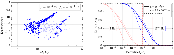
Figure 1: BBH eccentricities at $f_{\rm GW}=10^{-2}$Hz (left), evolved with a uniformly distributed $q\in\left[0.1,1\right]$ and the cloud on the heavier black hole. The pale blue dots account for the values without the cloud [15]. (BBHs with $e\lesssim 10^{-6}$ are not shown.) Cumulative values (right), with (solid) and without (dotted) the cloud, both at $10^{-2}\,\mathrm{Hz}$ (blue) and $1\,\mathrm{Hz}$ (pink), respectively.

Eccentric fixed point. For the GW-dominated epochs, with $r\simeq 1$, the leading order term in (Signatures of ultralight bosons in the orbital eccentricity of binary black holes) vanishes, and the first contribution is at ${\cal O}(e^{2})$. Likewise for the $k=0$ (main) resonance, for which the first term is $\propto\big{(}\tfrac{r}{2}-\tfrac{11}{3}\big{)}e^{2}$. As a result, the eccentricity is damped unless the orbit gets a large kick ($r\gtrsim 7.3$). As the influence of the cloud increases, the RHS of (Signatures of ultralight bosons in the orbital eccentricity of binary black holes) asymptotes (modulo a positive prefactor) to $(\mathfrak{f}_{k}-1)(r-1)$, in which case it enters at leading order. Moreover, the differences in the GW fluxes in (9) and (10) generate a distinction between the early and late resonances. In the floating case, with $r\simeq 0$, the eccentricity grows for the early resonances $(\mathfrak{f}_{k}<1)$ and decays for the late ones $(\mathfrak{f}_{k}>1)$. This can be understood by noticing that, when $\dot{E}_{\mathrm{o}}\simeq 0$, we have $\dot{L}_{\mathrm{o}}\propto\left(\tfrac{\Omega-\Omega_{0}}{\Omega\Omega_{0}}+\mathcal{O}(e^{2})\right),\,$ and using $d(L^{2}_{\mathrm{o}})\propto-d(e^{2})$ the eccentricity grows for $\Omega_{k}<\Omega_{0}$ and decays whenever $\Omega_{k}\geq\Omega_{0}$. This trend is reversed in the sinking case.

Due to the changes in the time evolution of the eccentricity across different resonances, it is instructive to look at the opposite limit $e\to 1$. In that case, the RHS of (Signatures of ultralight bosons in the orbital eccentricity of binary black holes) becomes $\propto\frac{r-1}{(1-e)^{3}}$. Let us consider the case of a floating orbit. Since the sign of $\frac{de}{dt}$ is positive for $\Omega_{k}<\Omega_{0}$, but turns negative when the eccentricity approaches $e\simeq 1$, this implies the existence of a critical “attractor” fixed point, $e_{\rm cr}$, given by the condition $g(e_{\rm cr})/f(e_{cr})=\mathfrak{f}_{k}$ [cf. (Signatures of ultralight bosons in the orbital eccentricity of binary black holes)]. For instance,

$$e_{\rm cr}=\{0.46,0.35,0.29\},\quad{\rm for}\quad|\Delta m|=\{1,2,3\}\,,$$ (17)

with $k=-1$. Similarly, an unstable fixed point develops for the earlier and main sinking resonances.

For the case of floating orbits (with $s\Delta m<0$), if the backreaction is sufficiently effective to enforce $r_{k}\simeq 0$ while the eccentricity approaches the critical point, one can then estimate the floating time $\Delta t_{\mathrm{FL}}\simeq b_{k}/\sqrt{\gamma_{k}}$, left-over population $|c_{a}(\infty)|^{2}\lesssim r_{k}$, and notably the growth of the eccentricity upon exiting the resonant transition,

$$e_{\mathrm{fin}}\simeq e_{\mathrm{cr}}\sqrt{1-\mathrm{e}^{-\mathrm{C_{k}}}}\,,\quad{\rm with}\,\,\mathrm{C_{k}}\sim\tfrac{\sqrt{\gamma_{k}}}{\Omega_{k}}b_{k}\,.$$ (18)

Although we have derived various analytic results under simplifying assumptions, we have demonstrated through numerical studies that the above behavior remains valid for generic (planar) orbits. See [46] and the supplemental material for details.

The cloud’s eccentric fossil. As it was argued in the literature [15, 17, 16], the distribution of masses and eccentricities observed with LISA can in principle distinguish between formation channels. However, the contrast between vacuum evolution and the large eccentricities produced by the cloud’s resonant transition can lead to dramatic changes in the expected evolution of the system. As a proof of concept, we take the stellar-mass BBH population studied in [15], with chirp masses ${\cal M}\lesssim 10M_{\odot}$, expected to form exclusively in isolation. We consider clouds of ultralight bosons of mass between $10^{-13}$ and $10^{-11}$ eV, in a planar (co-rotating) orbit with the parent black hole’s spin aligned with the orbital angular momentum. Superradiance may then excite the $\ket{322}$ state which, depending on black hole’s mass and birth orbital frequency, will experience a series of (hyper)fine transitions. To illustrate the distinct physical effects, and following [15, 14], we consider a birth orbital frequency (for the cloud+BBH system) at $\Omega_{\rm ini}/\pi\simeq 10^{-4}$Hz, and evolve until $f_{\rm GW}=10^{-2}$ and 1 Hz, with [68]

$$f_{\rm GW}\simeq\frac{\Omega}{\pi}\frac{(1+e)^{1.1954}}{(1-e^{2})^{3/2}}\,,$$ (19)

the peak GW frequency. The final distribution is shown on the left panel of Fig. 1. While some of the BBHs experience an early overtone of the hyperfine transition, the majority are affected by transitions through the fine overtones instead. The BBH then float over a period of time while increasing the orbital eccentricity. Moreover, the cloud typically either terminates there or decays later at the $k=0$ resonance. Depending on the parameters, the ultimate decay may either decrease the eccentricity or have a small impact on the orbit. As a result, a wedge-type distribution emerges, with the heavier black holes (within each wedge) subject to the largest increase in eccentricities.The cumulative effect (i.e. the ratio of binaries with $e$ above a reference eccentricity $e_{0}$) is shown on the right panel of Fig. 1, where a significant fraction of the population (with different parent masses) is affected by the resonances, yielding values of the eccentricities at 1Hz that may be within reach of mid-band and Decihertz detectors. As the value of $\mu$ increases (decreases) the location of the wedge in the distribution moves towards lower (higher) masses. The dependence on the value of $\mu$ for this population of BBH (with ${\cal M}\lesssim 10M_{\odot}$), reaching $e\gtrsim 10^{-2}$ at $f_{\rm GW}=10^{-2}\,$Hz, is shown in Fig. 2.

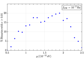
Figure 2: Percentage of binaries with eccentricities above 0.01 at $f_{\mathrm{GW}}=10^{-2}\,$Hz for different values of $\mu$.

Eccentric in band. Due to the connection to formation channels, we discussed a sub-population of BBHs. However, similar conclusions apply to black holes with higher masses [46]. For instance, for a GW170809-type event [69] (${\cal M}\simeq 24M_{\odot})$, with a parent black hole $M\simeq 20M_{\odot}$ and a (heavier) companion $M_{\star}\simeq 40M_{\odot}$, we find $f_{\rm GW}\gtrsim 10^{-2}$ Hz at the $k=-1$ fine transition for $\mu\simeq 1.5\times 10^{-12}$ eV. The BBH reaches the resonance and floats, with approximately constant orbital frequency for about six years, while the eccentricity increases from $e\lesssim 10^{-2}$ to $e\simeq 0.1$, and likewise the peak GW frequency grows, while the cloud depletes. The resulting frequency evolution till merger, which is distinct from the growth of the eccentricity that may occur due to other astrophysical mechanisms [70, 71], is displayed in Fig. 3. In addition to the notable features, higher harmonics would also become more relevant as the eccentricity increases [72]. As for the case of large tidal Love numbers [37, 42], new dedicated templates will be needed to search for these peculiar phenomena in the GW data.

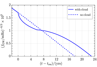
Figure 3: Evolution of the peak frequency through a resonant transition (at $t-t_{\mathrm{res}}=0$) in the LISA band of a GW170809-like event, compared to the evolution without the cloud.

Conclusions. We have shown that the presence of a boson cloud surrounding a black hole in a binary system can impact the distribution of masses and eccentricities observable with GW detectors. We have also found that a greater-than-expected value of the eccentricity, $e\gtrsim 10^{-2}$ at GW frequencies $f_{\rm GW}\simeq 10^{-2}$Hz, develops for a (sub-)population of isolated stellar-mass BBHs (with ${\cal M}\lesssim 10M_{\odot}$), right at the heart of the LISA band. Likewise, these BBHs will decay through GW emission to values of the eccentricities, i.e. $e\simeq 10^{-4}-10^{-3}$, within experimental reach of mid-band [6] and Decihertz [7] detectors. The observation of such GW signals would then provide tantalizing evidence for the existence of an ultralight particle of mass between $5\times 10^{-13}$ and $2.5\times 10^{-12}$ eV in nature. Furthermore, we have also shown that in-band resonance transitions are possible, yielding dramatic changes in the GW frequency evolution, constituting yet another smoking-gun signature of the imprint of a boson cloud in the BBH dynamics.

There are several venues for further exploration. Firstly, we have concentrated here on (co-rotating) transitions that are outside of the cloud, thus ignoring Bohr resonances altogether, which are subject to dynamical friction [40, 41]. Preliminary studies suggest that a similar increase of eccentricity occurs for certain type of transitions at higher frequencies, which would put them within reach of the ET and CE detectors [46], but a more in-depth study is needed. Secondly, we have considered aligned-spin BBHs. This is justified for the isolated populations. However, to encompass also dynamically-formed systems, we must add inclination and new (off-plane) transitions [41]. While our results remain unchanged for quasi-planar motion, we also expect similar conclusions to apply for inclined orbits (see [73] for related work). Finally, identical results can be drawn also for neutron star/black hole binaries. For instance, for those formed in isolation, the parent black hole mass is expected to be near $M\simeq 7M_{\odot}$, and likewise in binaries with negligible eccentricity at $f_{\rm GW}\simeq 1$Hz [13, 25, 31]. The presence of a boson cloud would then also lead to larger-than-expected eccentricities, providing additional circumstantial evidence for a new ultralight particle in nature.

Acknowledgements. While this letter was in preparation we learned of the related work in [73]. We thank G.M. Tomaselli for informative discussions and the authors of [73] for sharing a draft and coordinating the release. The work of MB and MK is supported in part by the Deutsche Forschungsgemeinschaft (DFG, German Research Foundation) under Germany’s Excellence Strategy – EXC 2121 “Quantum Universe” – 390833306. MB and RAP are supported in part by the ERC Consolidator Grant “Precision Gravity: From the LHC to LISA” provided by the European Research Council (ERC) under the European Union’s H2020 research and innovation programme (grant No. 817791).

Supplemental Material

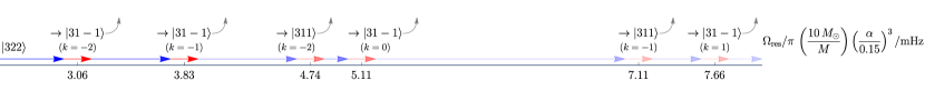
Figure 4: Orbital resonance frequencies of possible (fine) transitions for the $\ket{322}$-component of the cloud. The blue and red arrows represent vacuum and floating BBH evolution, respectively; whereas the grey arrows point to various (rapidly decaying) modes that ultimate deplete the cloud. The thinner the line the smaller the cloud gets.

Appendix A Gravitational atom

The range of ultralight masses that we probe yield a (very) high “axion decay constant” ($f_{a}$), generically suppressing self-interactions [74, 75, 76, 77] and coupling to other species [78, 79, 80, 81, 82]. In addition, for the black hole masses we studied, with $5M_{\odot}\lesssim M\lesssim 50M_{\odot}$, we arrive at small-to-moderate values of $\alpha\lesssim 0.25$, keeping relativistic corrections to the hydrogenic states small [55, 83, 60, 84]. In this regime, the eigenvalues are given by [37, 48]

$$\begin{split}\epsilon_{nlm}=&\,\mu\left(1-\tfrac{\alpha^{2}}{2n^{2}}-\left[\tfrac{1}{8n}+\tfrac{6}{2l+1}-\tfrac{2}{n}\right]\tfrac{\alpha^{4}}{n^{3}}\right.\\ &\left.+\tfrac{16}{2l(2l+1)(2l+2)}\tfrac{\tilde{a}m\alpha^{5}}{n^{3}}\right)\,.\end{split}$$ (20)

Furthermore, from Detweiler’s approximation [47, 48],

$$\Gamma_{nlm}\simeq 2\tilde{r}_{+}C_{nl}g_{lm}(\tilde{a},\alpha,\omega)(m\Omega_{H}-\omega_{nlm})\alpha^{4l+5},$$ (21)

with $C_{nl}\equiv\frac{2^{4l+1}(n+l)!}{n^{2l+4}(n-l-1)!}\left[\frac{l!}{(2l)!(2l+1)!}\right]^{2}$, $g_{lm}(\tilde{a},\alpha,\omega)\equiv\prod_{k=1}^{l}\left(k^{2}(1-\tilde{a}^{2})+(\tilde{a}m-2r_{+}\omega)^{2}\right)$ and $\tilde{r}_{+}\equiv 1+\sqrt{1-\tilde{a}^{2}}$, $\tilde{r}_{+}\equiv r_{+}/M$, and $\Omega_{H}\equiv\tilde{a}/(2r_{+})$; whereas for the cloud itself decaying into GWs, we use the (non-relativistic) approximation in [51].

Appendix B Tidal interactions

For equatorial orbits and resonances triggered away from the cloud, the tidal interaction is given by [37, 38]

$$\bra{b}V_{\star}\ket{a} \equiv \sum^{\infty}_{l_{\star}=2}\sum_{|m_{\star}|\leq l_{\star}}\eta_{ab}^{(\star)}\,,$$ (22)

$$\eta^{(\star)}_{ab} = -\frac{q\alpha}{r_{\mathrm{c}}}\mathsf{R}^{-(l_{\star}+1)}_{\star}\frac{4\pi}{2l_{\star}+1}Y^{\ast}_{(\star)}\left(\frac{\pi}{2},\varphi_{\star}\right)I_{r}I_{\Omega}\,,$$

$$I_{r} \approx \int^{\infty}d\mathsf{r}\mathsf{r}^{2}\hat{\mathcal{R}}_{b}\hat{\mathcal{R}}_{a}\mathsf{r}^{l_{\star}}\,$$ (23)

$$I_{\Omega} \equiv \int d\Omega Y^{\ast}_{b}(\theta,\phi)Y_{(\star)}(\theta,\phi)Y_{a}(\theta,\phi)\,,$$ (24)

where $(\star)\equiv(l_{\star},m_{\star})$, $\mathsf{r}\equiv r/r_{\mathrm{c}}$, $\hat{\mathcal{R}}_{c}=r_{\mathrm{c}}^{3/2}\mathcal{R}_{c}$ is the (dimensionless) hydrogenic radial wavefunction, $Y_{lm}$ is the spherical harmonic. We leave to [46] the discussion on resonances “inside the cloud”, including dipole-mediated transitions [85, 60, 84].

The Jacobi-Anger expansion,

$$e^{\pm i\Delta m(\vartheta+2e\sin(\vartheta))}=\sum_{k=-\infty}^{\infty}(\pm 1)^{k}J_{k}(2e\Delta m)\mathrm{e}^{i(k\pm\Delta m)\vartheta}\,,$$ (25)

can be applied to the off-diagonal terms of the Hamiltonian [cf. (3) in the main text]. Using the properties of the Bessel function , the tidal perturbation [cf. (6) of the main text] becomes

$$\eta^{(\star)}_{ab,k} = \eta_{0}\mathfrak{f}^{\frac{2}{3}(l_{\star}+1)}\frac{(\Delta me)^{|k|}}{|k!|}\left(1+\frac{(l_{\star}+1)k}{2\Delta m}\right)+\mathcal{O}(e^{|k|+1})\,,$$

$$\eta^{(\star)}_{ab,0} = \frac{q\alpha}{r_{\mathrm{c}}}\mathsf{R}^{-(l_{\star}+1)}_{0}\frac{4\pi}{2l_{\star}+1}\left|Y^{\ast}_{(\star)}\left(\frac{\pi}{2},\varphi_{\star}\right)\right|I_{r}I_{\Omega}\,.$$ (26)

This interaction is nonzero only if the selection rules are satisfied [37, 38]: $-m_{b}+m_{\star}+m_{a}=0$, $l_{b}+l_{\star}+l_{a}=2p$, $|l_{a}-l_{b}|\leq l_{\star}\leq l_{a}+l_{b}$. Furthermore, for equatorial orbits, for even (odd) $l_{\star}$ only the spherical harmonics even (odd) in $m_{\star}\neq 0$ are nonzero.

Appendix C Atomic resonances

As the populated state has a maximal azimuthal number $m_{\mathrm{max}}=n-1$, at the (hyper)fine resonances, it can only transition into states with lower $m$. Such transitions are only possible on co-rotating orbits, where they obey $s\Delta m<0$, yielding floating-type motion. From the selection rules for the tidal interactions, the $\ket{211}$ state has only one hyperfine transition to $\ket{21-1}$, while the only possible fine transition, to $\ket{200}$, can only occur inside the cloud. Furthermore, for small values of $\alpha$, we find that the floating time of this transition would take longer than a Hubble time, preventing them to reach the LISA band. At the same time, (barring a precise fine tuning of the birth frequency of the BBH+cloud) for large values of $\alpha$ we expect the $\ket{211}$ component of the cloud to decay through its own GW emission before reaching the resonant transition (see also [62, 86]). On the other hand, the (longer-lived) $\ket{322}$ state may experience various types of resonances. In contrast to early and late resonances with $k=\pm 1$, all of the $k=0$ hyperfine transitions to $\ket{32m}$ happen at the same frequency ($\Delta m$ drops out of the ratio). The dominant main (hyperfine) transition is the one to $\ket{320}$, with $l_{\star}=2$ [as the $\ket{322}\to\ket{32-2}$ resonance can only be mediated by the hexadecapole ($l_{\star}=4$), making it extremely weak and nonadiabatic]. Transitions to the $\ket{32\pm 1}$ states are not possible for equatorial orbits. The fine resonances from the excited state are (octopolar) to the $\ket{31-1}$, $\ket{311}$ and (quadrupolar) $\ket{300}$ states, in that order in the frequency domain. We show a succession of transitions in Fig. 4. We ignored the (sinking) high-$l_{\star}$ Bohr resonances that can overlap with the range of frequencies that we consider here, since they do not significantly affect the dynamical evolution. We postpone the general analysis of Bohr transitions to [46].

Appendix D Nonlinear Landau-Zener transition

Linear solution

The solution of the (linear) LZ transition with $\dot{\Omega}_{k}\simeq f(e)\gamma_{k}$ $\simeq\mathrm{const}$, including a decaying width, is given by [59, 61, 62] (see also [58, 38])

$$|c_{a}|^{2} = \exp\left(-v_{k}\tau-\frac{\pi}{2}z_{k}\right)\left|D_{iz_{k}}\left(e^{i\frac{3\pi}{4}}\left(\tau-iv_{k}\right)\right)\right|^{2}$$ (27)

$$|c_{b}|^{2} = \exp\left(-v_{k}\tau-\frac{\pi}{2}z_{k}\right)z_{k}\left|D_{iz_{k}-1}\left(e^{i\frac{3\pi}{4}}\left(\tau-iv_{k}\right)\right)\right|^{2}\,,$$

where $D$ are parabolic cylinder functions [58], and we introduced a dimensionless time

$$\tau\equiv t\sqrt{|\Delta m+k|f(e)\gamma_{k}}\,.$$ (28)

Remarkably, the transition probability at infinity, $|c_{a}(\infty)|^{2}=\mathrm{e}^{-2\pi z_{k}}$, is independent of $v_{k}$.

In general, the presence of a decay width tends to smooth the LZ transition, by transferring a fraction of the initial state earlier than the case with $v_{k}=0$, and also by damping late-time oscillations. Consequently, for large widths, $\tfrac{d}{d\tau}|c_{a}|^{2}$ peaks earlier than the $v_{k}=0$ case. In the limit $v_{k}\gg z_{k}$, the LZ solution acquires a simple form [61, 62]

$$|c_{a}|^{2} = \exp\left[-2z_{k}\left(\arctan\left(\frac{\tau}{v_{k}}\right)+\frac{\pi}{2}\right)\right]\,,$$ (29)

$$|c_{b}|^{2} = |c_{a}|^{2}\frac{z_{k}}{\tau^{2}+v_{k}^{2}}\,.$$ (30)

In this regime, $\tfrac{d}{d\tau}|c_{a}|^{2}$ peaks at $\tau_{\mathrm{max}}\simeq-z_{k}v_{k}$, and the width of the transition roughly scales as

$$\frac{\Delta\Omega}{\sqrt{|\Delta m+k|f(e)\gamma}}\simeq 2v_{k}\sqrt{1+2z_{k}^{2}}\,.$$ (31)

Balance equations

In the two-level system with a decaying mode, we can relate the total energy and the angular momentum of the $\ket{a,b,\mathrm{BH}}$ state as [cf. (9)-(11) in the main text]

$$(\dot{L}_{\mathrm{c}}+\dot{S}) = (\dot{E}_{\mathrm{c}}+\dot{M})\frac{\Delta m}{\Delta\epsilon}\times\frac{\rho_{\epsilon}(t)}{\rho_{m}(t)}$$ (32)

$$\rho_{x} \equiv \frac{x_{a}}{\Delta x}\frac{d}{dt}|c_{a}|^{2}-\Gamma_{a}|c_{a}|^{2}-\sum\hat{\Gamma}_{a}|c_{a}|^{2}$$ (33)

$$+(a\to b)\,,$$

where $x\equiv\left\{\epsilon,m\right\}$, and the $\hat{\Gamma}$ represents other sources of dissipation, such as GW emission from the cloud [9, 51, 52, 53, 54, 55] or ionization [39, 40, 41]. From the Schrödinger equation [cf. (3)], we find

$$\rho_{x}=\frac{d}{dt}|c_{a}|^{2}+2|c_{a}|^{2}\Gamma_{a}+2\frac{x_{b}}{\Delta x}\sum\left(\hat{\Gamma}_{a}|c_{a}|^{2}+\hat{\Gamma}_{b}|c_{b}|^{2}\right)\,,$$

and a similar equation applies with $a\leftrightarrow b$. After superradiance saturates the growth of the cloud in the $\ket{a}$ state, we have $\Gamma_{a}\simeq 0$. Moreover, for the floating time of the resonances we consider here, we can ignore other sources of dissipation during the LZ transition (setting $\hat{\Gamma}\simeq 0$) [46]. Hence, $\rho_{x}=(d/dt)|c_{a}|^{2}$, which implies $\rho_{\epsilon}/\rho_{m}=1$, yielding the expression in (12)-(Signatures of ultralight bosons in the orbital eccentricity of binary black holes) of the main text.

Nonlinear backreaction effects

Because of the backreaction on the orbital frequency, which in turns controls the LZ transition, the problem becomes nonlinear, and it depends on the level-occupancy through the derivative of the parent state occupancy [cf. (13) in the main text]. We plot the this derivative for the linear LZ problem in Fig. 5. In the parts of the parameter space where it has compact support, the backreaction simply renormalizes the parameters $(z_{k},v_{k})\to$ $(\zeta_{k},w_{k})$ [cf. (Signatures of ultralight bosons in the orbital eccentricity of binary black holes) of the main text] near the maximum value, as

$$\zeta_{k}=\frac{\eta_{k}^{2}}{|\Delta m+k|\dot{\Omega}_{k}}=\frac{\eta_{k}^{2}}{|\Delta m+k|\gamma_{k}f(e)r}=\frac{z_{k}}{r_{k}(\zeta_{k})}\,,$$ (34)

and with the energy transfer itself depending on the level-occupancy of the cloud. The solution can, nonetheless, be found self-consistently in terms of the relevant parameters.

This mapping provides a useful indicator, even in the regime of strong backreaction, to evaluate whether, e.g., floating can occur, by indicating the breakdown of the linearization of the full problem. From the self-consistency condition (34) the “true” time scale for the nonlinear problem follows $\mathrm{T}=\sqrt{r_{k}}\tau$ . The LZ function derivatives can now be expressed in terms these quantities,

$$\frac{d|c_{i}|^{2}}{d\tau}=\sqrt{\frac{z_{k}}{\zeta_{k}}}\frac{d|c_{i}|^{2}}{d\mathrm{T}}\,,$$ (35)

leading to

$$-\frac{d|c_{a}|^{2}}{d\tau}\Big{|}_{\tau=-\zeta_{k}w_{k}}=\sqrt{\frac{z_{k}}{\zeta_{k}}}\psi_{k}(\zeta_{k},w_{k})\,,$$ (36)

$$\psi_{k}\equiv\frac{1}{2}e^{-\frac{1}{2}(\pi\zeta_{k})}\Bigg{[}2w_{k}\left|\mathcal{C}H_{i\zeta}\left(\frac{\mathcal{C}w_{k}\Delta w_{k}}{2}\right)\right|^{2}-$$

$$\quad\left(\mathcal{C}H_{1-i\zeta}\left(\frac{\mathcal{C}^{\ast}\Delta w_{k}^{\ast}}{2}\right)H_{i\zeta}\left(\frac{\mathcal{C}\Delta w_{k}}{2}\right)+\mathrm{c.c.}\right)\Bigg{]}\,,$$

where $\mathcal{C}=1+i$, $\Delta w_{k}=w_{k}(1-i\zeta_{k})$ and $H$ is the Hermite function. In what follows, for the sake of notation brevity, we take the small-eccentricity approximation, with $f(e)\simeq 1$. This is also justified by the fact that the eccentricity before the LZ transition is typically small across the parameter space, which we use to evaluate the type of transition the cloud will experience.

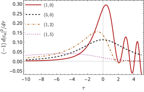
Figure 5: (Negative) derivative of the parent state occupancy, evaluated for a linear LZ transition. Brackets in the legend correspond to $(z_{k},v_{k})$. Note the decrease, and shift to the left, of the amplitude, as well as the widening of the function and damping of the late-time oscillations, as the ratio $v_{k}/z_{k}$ increases.

Negligible-decay regime

The $\psi_{k}$ function simplifies in the asymptotic regime

$$\lim_{\zeta\to 0}\psi_{k}\sim\sqrt{\pi}\zeta\,,\,\,\And\,\,\lim_{\zeta\to\infty}\psi_{k}\sim\frac{1}{4\sqrt{\zeta}}\,\quad(w_{k}\ll\zeta_{k})\,,$$

in which

$$\zeta_{k}\sim z_{k}\left(1-\mathrm{sgn}(s\Delta m)\frac{b_{k}}{4\sqrt{z_{k}}}\right)\,,$$ (37)

and the value of $r_{k}$ given in (16) of the main text. As advertised, the energy transfer for the adiabatic floating $(s\Delta m<0)$, is extremised by large values of $b_{k}$ with moderate $z_{k}$ parameters. In contrast, sinking $(s\Delta m>0)$ is consistent with large adiabaticity only for moderate backreaction $b_{k}<4\sqrt{z}_{k}$. Furthermore, the large backreaction limit $(b_{k}\gg 1)$ of the weakly-adiabatic regime

$$\zeta_{k}\sim\mathrm{sgn}(s\Delta m)\left(\frac{z_{k}}{b^{2}_{k}\pi}\right)^{1/3}\,,\,r_{k}\sim\mathrm{sgn}(s\Delta m)(\pi b^{2}_{k}z^{2}_{k})^{1/3}\,,$$

is only possible for sinking orbits. In such scenarios, the strong backreaction then mostly leads to nonadiabatic sinking transitions, with a potentially significant impact on the orbit

Strong-decay regime

In general, the impact of the decay width depends on the dynamical timescale of the LZ transition and should be compared with the strength of the coupling. Moreover, for eccentric orbits, even if $z_{0}>v_{0}$ at $\mathfrak{f}_{0}=1$, this hierarchy may be reversed for $\mathfrak{f}_{k}\neq 1$, due to the $e^{2|k|}$ suppression in $z_{k}$. Similarly to the case of negligible decay, we can also obtain approximate relations in the limit described by (29), yielding

$$\psi_{k} \sim \frac{2\zeta_{k}\mathrm{e}^{-\zeta_{k}\left[\pi-2\arctan(\zeta_{k})\right]}}{w_{k}(\zeta_{k}^{2}+1)}\,,$$ (38)

$$r_{k} \sim 1\pm 2b_{k}z_{k}\frac{\mathrm{e}^{-\zeta_{k}\left[\pi-2\arctan(\zeta_{k})\right]}}{v_{k}(\zeta_{k}^{2}+1)}\,.$$ (39)

In general, this regime shares various qualitative behavior as in the $w_{k}\ll\zeta_{k}$ case, but with the adiabaticity gain/loss and orbital impact suppressed by the ratio $b_{k}/v_{k}$. In particular, large adiabaticity is consistent only for floating orbits, where we have

$$\zeta_{k}\simeq\frac{\sqrt{2}}{\mathrm{e}}\sqrt{\frac{b_{k}z_{k}}{v_{k}}}\,,\quad r_{k}=\frac{z_{k}}{\zeta_{k}}\to 0\,.\quad(b_{k}\gg 1)$$

In contrast, for sinking orbits, the strong backreaction requires a small population transfer, and we find

$$\zeta_{k}\simeq\frac{v_{k}}{2b_{k}}\,,\quad r_{k}\simeq\frac{2b_{k}z_{k}}{v_{k}}\gg 1\,.\quad(b_{k}\gg 1)$$

Notice that, somewhat counter-intuitively, a strong-decay width not only does not necessarily imply the total depletion of the cloud, instead it suppresses $r_{k}$, hence the ability of the system to float, resulting in a lesser amount of the cloud being transferred to the decaying mode (see (48) below).

Appendix E Floating

For values of the energy transfer $r_{k}\lesssim 0.2$, the growth of the orbital frequency is sufficiently suppressed to allow for the possibility of floating. In that case, the growth of (initially small) eccentricity is given, in units of the dynamical time introduced in (31), by

$$e(t) \simeq \sqrt{e^{2}_{\mathrm{in}}+I_{e}\tau(1-\mathfrak{f}_{k})}\,,\quad\quad\quad(\mathfrak{f}_{k}\neq 1)$$ (40)

$$e(t) \simeq e_{\mathrm{in}}\exp{-\frac{11}{6}I_{e}\tau}\,,\quad\quad\quad\,\,(\mathfrak{f}_{k}=1)$$ (41)

$$I_{e} \equiv \frac{2}{3}\frac{\sqrt{\gamma_{0}}}{\Omega_{0}}\frac{\mathfrak{f}^{5/6}_{k}}{|\Delta m+k|^{1/2}}\,.$$

The critical points of the evolution of the eccentricity depend both on $|\Delta m|$ and $|k|$. For the first few values of $|k|$ they are described by the polynomial fit $e_{\mathrm{cr}}=g_{0}+g_{1}k+g_{2}k^{2}$, where $g_{0}=\{0.3,0.2,0.16\}$, $g_{1}=\{0.18,0.16,0.14\}$, $g_{2}=\{2,1.6,1.3\}\times 10^{-2}$, all for $|\Delta m|=\{1,2,3\}$ in respective order.

To calculate the evolution of the eccentricity towards the fixed point, we change the time variable in the evolution equations [cf. (Signatures of ultralight bosons in the orbital eccentricity of binary black holes)], from $t$ to $e^{2}(t)$, yielding

$$\int^{e^{2}_{\mathrm{fin}}}_{e^{2}_{\mathrm{in}}}\frac{d(e^{2})}{\sqrt{1-e^{2}}\left[\frac{g(e)}{f(e)}-\mathfrak{f}_{k}\right]}=I_{e}b_{k}\left(1-|c_{a}(\infty)|^{2}\right)\,,$$ (42)

The result can then be approximated by (18) in the main text, where

$$\mathrm{C}_{k}=c_{\Delta m,k}\left[I_{e}b_{k}\left(1-|c_{a}(\infty)|^{2}\right)+\frac{e^{2}_{\mathrm{in}}}{1-\mathfrak{f}_{k}}\right]\,,$$ (43)

and $c_{\Delta m,-1}=$ $\{2.37,2,1.37\}$ for $\Delta m=\{-1,-2,-3\}$. From the value of $e^{2}_{\mathrm{fin}}$ in (42), we can also estimate the duration of the floating period

$$\Delta\tau_{\mathrm{Fl}} = \frac{1}{I_{e}}\int^{e^{2}_{\mathrm{fin}}}_{e^{2}_{\mathrm{in}}}d(e^{2})\frac{1}{\sqrt{f(e)}\sqrt{1-e^{2}}\left[\frac{g(e)}{f(e)}-\mathfrak{f}_{k}\right]}\,,$$ (44)

$$\simeq \frac{\mathrm{C}_{k}}{\tilde{c}_{\Delta m,k}I_{e}}\,,\quad\frac{c_{\Delta m,k}}{\tilde{c}_{\Delta m,k}}=\frac{1}{\sqrt{f(e_{\mathrm{cr}})}}\,.$$

An exemplary parameter space of final eccentricity and floating time is shown in Fig. 6.

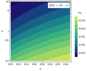
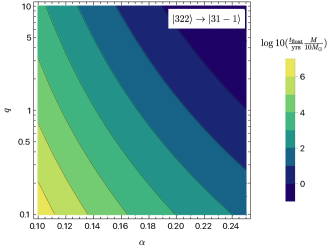
Figure 6: Final eccentricity (left) and floating time (right), for the $\ket{322}\to\ket{31-1}$ transition with $k=-1$, assuming initial conditions that lead to a (long-lasting) floating orbit ($r_{-1}\simeq 0$) and $e_{\mathrm{in}}\ll 1$.

Strong floating provides a distinct phase of the non-linear LZ transition, during which typically most of the population transfer occurs. From (12) of the main text, we have

$$\frac{d|c_{a}|^{2}}{d\tau}=\frac{r(\tau)-1}{b_{k}}\,,$$ (45)

yielding a linear-in-time decay of the population during floating, and a transfer of population given by

$$|c_{a}(\infty)|^{2}\simeq|c_{a}(\tau<\mathrm{Fl})|^{2}-(1-r_{k})\frac{\Delta\tau_{\rm Fl}}{b_{k}}\,.$$ (46)

In the strong decay regime, the condition $r(t)\to 0$ at the resonance is necessary at each point in time, but not sufficient to guarantee a steady floating-type period. In addition, there must be enough of the cloud left to sustain a small $r(t)$. Following [62], one can estimate the sufficient condition by considering the minimum amount of cloud needed to “startjump” a floating period. Applying the linear LZ solution (29) in  (13) of the main text, we find

$$|c_{a}|^{2}_{\mathrm{min}}\simeq\frac{v_{k}\sqrt{f(e_{\mathrm{in}})}}{2b_{k}z_{k}(e_{\rm in})}(1-r_{k})\,.$$ (47)

The left hand side can be interpreted as the minimal amount of cloud needed to start floating at a particular resonance. In turn, if the right hand side is larger than one, floating cannot start. The same condition can also be used to estimate the amount of cloud left when floating stops, by matching into the linear LZ solution backwards, from the end of the floating time,

$$|c_{a}(\infty)|^{2}\simeq\frac{v_{k}\sqrt{f(e_{\mathrm{fin}})}}{2b_{k}z_{k}(e_{\mathrm{fin}})}(1-r_{k})\,,$$ (48)

which then becomes the portion of the cloud surviving after floating stops. Strong decay and small $z_{k}$ could in principle interrupt the floating period and leave a moderate amount of the cloud intact.

However, at the overtones we have $z_{k}\sim e^{|2k|}$, which is increasing during floating. Hence, as the eccentricity approaches the critical point, for instance at the $k=-1$ overtone, the value of $z_{k}$ increases by a factor $\left(e_{\rm cr}/e_{\rm in}\right)^{2}\simeq 10^{2}-10^{3}$, thus significantly extending the floating period, and reducing the amount of cloud left after the transition, in comparison with the naïve estimate in (47).

In general, the equations in (42), (44) and (48) must be solved self-consistently in order to determine the end state of floating. As an estimate, we may apply (40) to (48), and assuming $e_{\mathrm{in}}\ll 1$, we have

$$\frac{\Delta\tau_{\mathrm{Fl}}}{b_{k}/\sqrt{f(e_{\mathrm{cr}})}}\simeq\left(\frac{x-1}{2x}+\sqrt{\frac{(x+1)^{2}}{4x^{2}}-\frac{\lambda}{x}}\right)\,,$$ (49)

$$\lambda=\frac{v_{k}}{2b_{k}z_{k}(e_{\mathrm{in}})}\,,\quad x=\frac{I_{e}b_{k}(1-f_{k})}{e^{2}_{\mathrm{in}}}\,.$$

Notice that for the $k=-1$ overtone, the dependence on $e_{\mathrm{in}}$ drops out from the ratio $\lambda/x$. In this case $\lambda\ll x$, and we find the longest periods of floating, $\Delta\tau_{\rm Fl}\simeq b_{k}/\sqrt{f(e_{\rm cr})}$, and largest depletion of the $|c_{a}(\infty)|^{2}\lesssim r_{k}$. Depending on the resonances and the parameter space, such hierarchy may be also valid for higher overtones.

Appendix F Numerical validation

For generic orbits, the instantaneous position can be expressed as $R_{\star}=a(1-e\cos{u})$, as a function of the eccentric anomaly $u$. The eccentric anomaly is then related to the mean anomaly via Kepler’s equation $u-e\sin(u)=\vartheta$ (e.g. [56]). We have validated the analytic results obtained using the small-eccentricity approximation by numerically solving the Schrödinger equation for arbitrary (planar) orbits, coupled with the energy-momentum balance equations [cf. (3),(9)-(11) of the main text], for a number of representative examples. We use the NDSolve routine in Mathematica [87], monitoring the violation of unitarity in the $\Gamma_{b}=0$ regime, residual for $\Gamma_{b}\geq 0$, as well as the state occupation numbers (27). We have also checked the consistency of our results by comparing with the values in [48] for $(e,\Gamma_{b})=0$.

In general, the numerical results are broadly consistent with the analytical arguments. As expected, the largest discrepancy occurs for the estimates of $r(t)$ and $|c_{a}(\infty)|^{2}$. For the floating regime, the analytic results tend to overestimate their respective values by a factor of few to an order of magnitude. Hence, our conclusions based on the analytic approximations err on the side of caution. In Fig.  7 we present (left) the numerical eccentricity evolution of a two-level system with $\Delta m=2$ for values $\{z_{0}=4,v_{0}=2,b_{0}=200,e_{0}=10^{-2}\}$, at the main resonance. For these parameters, we have $\{z_{-1}=7\cdot 10^{-3},v_{-1}=3.4,b_{-1}=450,I_{e}=2\cdot 10^{-4}\}$ at the $k=-1$ overtone, for which one finds a strong-decay regime: $v_{-1}/z_{-1}=512$. We start the numerical evaluation before the first overtone, following also the case $v_{-1}=0$. Away from the resonance, the orbital evolution closely follows standard GW evolution in vacuum. The approximations from Sec. D then correctly predict the strong floating that occurs (in both setups) at the frequency given by (8). Notice that, modulo small deviations, both cases follow the $r_{k}\simeq 0$ prediction for the eccentricity growth in (42). Furthermore, broadly consistent with our estimates, the left-over occupancy of the inital state is given by $|c_{a}(\infty)|^{2}\simeq 10^{-4}$ and $|c_{a}(\infty)|^{2}\simeq 10^{-3}$, with and without the decay, respectively. Finally, reducing the backreaction to $b_{0}=25$ (Fig. 7, right), the decaying case does not develop floating as $r_{k}\simeq 0.8$, although as expected, eccentricity will still grow slightly and the transfer of population is somewhat increased compared to the linear LZ transition. In contrast, the non-decaying case still exhibits a strong floating, follows the predicted growth of the eccentricity and transfers the parent state up to $|c_{a}(\infty)|^{2}\simeq 5\times 10^{-3}$.

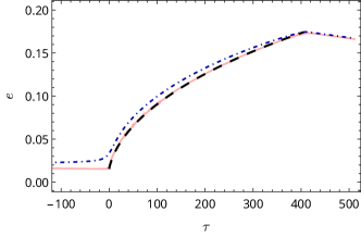
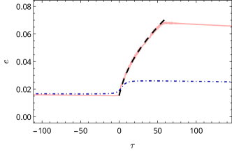
Figure 7: Full numerical evolution of the two examples described in App. F. The two figures correspond to the same $z_{k}$ but different values for $b_{k}$ (on the left is a few times larger than on the right). The curves show the evolution in the regime of vanishing (pink), and large decay $v_{k}\gg z_{k}$ (blue, dot-dashed), contrasted against the semi-analytic solution for the eccentricity evolution in the $r_{k}=0$ limit (black, dashed) [cf. (Signatures of ultralight bosons in the orbital eccentricity of binary black holes) in the main text].

Appendix G Eccentricity distribution

To evaluate the distribution of eccentricities in the population from [15], we order (in frequency) all possible hyperfine and fine resonances with the corresponding overtones, up to $|k|=5$. (A subset is displayed in Fig. 1.) We then calculate the corresponding parameters $(z_{k},v_{k},b_{k})$ for every resonance the cloud may encounter. The condition that the initial state had enough time to reach the resonance is imposed, constrained by the lifetime imposed by its own GW emission. We evolve in vacuum via [43, 44] between transitions. At every resonance, we estimate $r_{k}$ as explained in App. D, and from there the floating time, eccentricity growth, and left-over cloud, as explained in App. E. We use a cutoff at $10^{-3}$ of the initial $M_{c,0}/M$, to estimate when the cloud’s influence on the orbital dynamics becomes negligible.

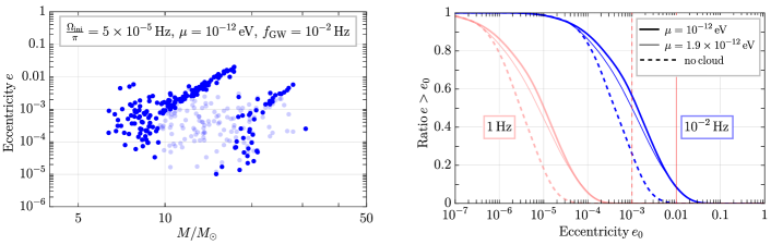
Figure 8: Same as Fig. 1, but with $\Omega_{\mathrm{ini}}/\pi=5\times 10^{-5}$ as the birth orbital frequency for the BBH+cloud system.

For the BBHs shown in Fig. 1, only a few percent experience a floating transition $\ket{322}\to\ket{31-1}$ with $k<-1$, while $25\,\%$ float at the $k=-1$ resonance, making it the dominant one. Approximately $15\,\%$ of the population float at the $k=0$ transition. Only a few experience resonances to $\ket{311}$ or $\ket{300}$ states. The black holes with the largest masses, hence largest values of $\alpha$ for fixed $\mu$, can float at the $\ket{320}$ hyperfine transition, where of the order of $5\,\%$ (each), see the main or $k=1$ resonance and decrease eccentricity there; or see an earlier resonance, and increase eccentricity instead. In general, hyperfine transitions correspond to the weak-decay regime, while fine transitions are typically of the strong-decay type.

Birth frequency

Similar to Fig. 1, we show in Fig. 8 the eccentricity distribution at $f_{\rm GW}=10^{-2}\,$Hz, but with a lower birth frequency for the BBH+cloud system, at $\Omega_{\mathrm{ini}}/\pi=5\times 10^{-5}\,$Hz. Although the number of larger-than-expected eccentricity points is somewhat lower, the plot illustrates the robustness of our predictions against changes in the initial conditions. In general, a large portion of BBHs that merge within a Hubble time will be born with orbital frequencies between $[0.5,1]\times 10^{-5}$Hz  [14]. Moreover, BBHs that are formed through a common-envelope mechanism that can bring the binary closer, e.g. [67], at the same time may produce a (younger) secondary black hole that can ultimately carry the boson cloud, pushing the cloud’s birth frequency towards higher values, thus avoiding altogether ($k=0$) hyperfine transitions that can decrease the eccentricity. Overall, our findings demonstrate that a skewed-type distribution and larger-than-expected eccentricities are robust predictions of the presence of boson clouds in the BBH dynamics.

References

- Abbott et al. [2023] R. Abbott et al. (KAGRA, VIRGO, LIGO Scientific), Open Data from the Third Observing Run of LIGO, Virgo, KAGRA, and GEO, Astrophys. J. Suppl. 267, 29 (2023), arXiv:2302.03676 [gr-qc] .
- Alves Batista et al. [2021] R. Alves Batista et al., EuCAPT White Paper: Opportunities and Challenges for Theoretical Astroparticle Physics in the Next Decade, (2021), arXiv:2110.10074 [astro-ph.HE] .
- Arun et al. [2022] K. G. Arun et al. (LISA), New horizons for fundamental physics with LISA, Living Rev. Rel. 25, 4 (2022), arXiv:2205.01597 [gr-qc] .
- Maggiore et al. [2020] M. Maggiore et al., Science Case for the Einstein Telescope, JCAP 03, 050, arXiv:1912.02622 [astro-ph.CO] .
- Reitze et al. [2019] D. Reitze et al., Cosmic Explorer: The U.S. Contribution to Gravitational-Wave Astronomy beyond LIGO, Bull. Am. Astron. Soc. 51, 035 (2019), arXiv:1907.04833 [astro-ph.IM] .
- Baum et al. [2023] S. Baum, Z. Bogorad, and P. W. Graham, Gravitational Wave Science in the Mid-Band with Atom Interferometers, (2023), arXiv:2309.07952 [gr-qc] .
- Kawamura et al. [2021] S. Kawamura et al., Current status of space gravitational wave antenna DECIGO and B-DECIGO, PTEP 2021, 05A105 (2021), arXiv:2006.13545 [gr-qc] .
- Arvanitaki et al. [2010] A. Arvanitaki, S. Dimopoulos, S. Dubovsky, N. Kaloper, and J. March-Russell, String Axiverse, Phys. Rev. D 81, 123530 (2010), arXiv:0905.4720 [hep-th] .
- Arvanitaki and Dubovsky [2011] A. Arvanitaki and S. Dubovsky, Exploring the String Axiverse with Precision Black Hole Physics, Phys. Rev. D 83, 044026 (2011), arXiv:1004.3558 [hep-th] .
- Marsh [2016] D. J. E. Marsh, Axion Cosmology, Phys. Rept. 643, 1 (2016), arXiv:1510.07633 [astro-ph.CO] .
- Demirtas et al. [2020] M. Demirtas, C. Long, L. McAllister, and M. Stillman, The Kreuzer-Skarke Axiverse, JHEP 04, 138, arXiv:1808.01282 [hep-th] .
- Mehta et al. [2021] V. M. Mehta, M. Demirtas, C. Long, D. J. E. Marsh, L. McAllister, and M. J. Stott, Superradiance in string theory, JCAP 07, 033, arXiv:2103.06812 [hep-th] .
- Belczynski et al. [2001] K. Belczynski, V. Kalogera, and T. Bulik, A Comprehensive study of binary compact objects as gravitational wave sources: Evolutionary channels, rates, and physical properties, Astrophys. J. 572, 407 (2001), arXiv:astro-ph/0111452 .
- Kowalska et al. [2011] I. Kowalska, T. Bulik, K. Belczynski, M. Dominik, and D. Gondek-Rosinska, The eccentricity distribution of compact binaries, Astronomy & Astrophysics 527, A70 (2011).
- Breivik et al. [2016] K. Breivik, C. L. Rodriguez, S. L. Larson, V. Kalogera, and F. A. Rasio, Distinguishing Between Formation Channels for Binary Black Holes with LISA, Astrophys. J. Lett. 830, L18 (2016), arXiv:1606.09558 [astro-ph.GA] .
- Nishizawa et al. [2016] A. Nishizawa, E. Berti, A. Klein, and A. Sesana, eLISA eccentricity measurements as tracers of binary black hole formation, Phys. Rev. D 94, 064020 (2016), arXiv:1605.01341 [gr-qc] .
- Nishizawa et al. [2017] A. Nishizawa, A. Sesana, E. Berti, and A. Klein, Constraining stellar binary black hole formation scenarios with eLISA eccentricity measurements, Mon. Not. Roy. Astron. Soc. 465, 4375 (2017), arXiv:1606.09295 [astro-ph.HE] .
- Rodriguez et al. [2016] C. L. Rodriguez, M. Zevin, C. Pankow, V. Kalogera, and F. A. Rasio, Illuminating Black Hole Binary Formation Channels with Spins in Advanced LIGO, Astrophys. J. Lett. 832, L2 (2016), arXiv:1609.05916 [astro-ph.HE] .
- Rodriguez et al. [2018a] C. L. Rodriguez, P. Amaro-Seoane, S. Chatterjee, and F. A. Rasio, Post-Newtonian Dynamics in Dense Star Clusters: Highly-Eccentric, Highly-Spinning, and Repeated Binary Black Hole Mergers, Phys. Rev. Lett. 120, 151101 (2018a), arXiv:1712.04937 [astro-ph.HE] .
- Rodriguez et al. [2018b] C. L. Rodriguez, P. Amaro-Seoane, S. Chatterjee, K. Kremer, F. A. Rasio, J. Samsing, C. S. Ye, and M. Zevin, Post-Newtonian Dynamics in Dense Star Clusters: Formation, Masses, and Merger Rates of Highly-Eccentric Black Hole Binaries, Phys. Rev. D 98, 123005 (2018b), arXiv:1811.04926 [astro-ph.HE] .
- Lower et al. [2018] M. E. Lower, E. Thrane, P. D. Lasky, and R. Smith, Measuring eccentricity in binary black hole inspirals with gravitational waves, Phys. Rev. D 98, 083028 (2018), arXiv:1806.05350 [astro-ph.HE] .
- Randall and Xianyu [2021] L. Randall and Z.-Z. Xianyu, Eccentricity without Measuring Eccentricity: Discriminating among Stellar Mass Black Hole Binary Formation Channels, Astrophys. J. 914, 75 (2021), arXiv:1907.02283 [astro-ph.HE] .
- Fang et al. [2019] X. Fang, T. A. Thompson, and C. M. Hirata, The Population of Eccentric Binary Black Holes: Implications for mHz Gravitational Wave Experiments, Astrophys. J. 875, 75 (2019), arXiv:1901.05092 [astro-ph.HE] .
- Romero-Shaw et al. [2020] I. M. Romero-Shaw, P. D. Lasky, E. Thrane, and J. C. Bustillo, GW190521: orbital eccentricity and signatures of dynamical formation in a binary black hole merger signal, Astrophys. J. Lett. 903, L5 (2020), arXiv:2009.04771 [astro-ph.HE] .
- Sedda [2020] M. A. Sedda, Dissecting the properties of neutron star - black hole mergers originating in dense star clusters, Commun. Phys. 3, 43 (2020), arXiv:2003.02279 [astro-ph.GA] .
- Glanz and Perets [2021] H. Glanz and H. B. Perets, Common envelope evolution of eccentric binaries, Monthly Notices of the Royal Astronomical Society 507, 2659 (2021), arXiv:2105.02227 [astro-ph.SR] .
- Zevin et al. [2021] M. Zevin, I. M. Romero-Shaw, K. Kremer, E. Thrane, and P. D. Lasky, Implications of Eccentric Observations on Binary Black Hole Formation Channels, Astrophys. J. Lett. 921, L43 (2021), arXiv:2106.09042 [astro-ph.HE] .
- Gualandris et al. [2022] A. Gualandris, F. M. Khan, E. Bortolas, M. Bonetti, A. Sesana, P. Berczik, and K. Holley-Bockelmann, Eccentricity evolution of massive black hole binaries from formation to coalescence, Monthly Notices of the Royal Astronomical Society 511, 4753–4765 (2022).
- Garg et al. [2023] M. Garg, S. Tiwari, A. Derdzinski, J. G. Baker, S. Marsat, and L. Mayer, The minimum measurable eccentricity from gravitational waves of LISA massive black hole binaries, (2023), arXiv:2307.13367 [astro-ph.GA] .
- Saini [2023] P. Saini, Resolving the eccentricity of stellar mass binary black holes with next generation ground-based gravitational wave detectors 10.1093/mnras/stae037 (2023), arXiv:2308.07565 [astro-ph.HE] .
- Dhurkunde and Nitz [2023] R. Dhurkunde and A. H. Nitz, Search for eccentric NSBH and BNS mergers in the third observing run of Advanced LIGO and Virgo, (2023), arXiv:2311.00242 [astro-ph.HE] .
- Zel’Dovich [1971] Y. B. Zel’Dovich, Generation of Waves by a Rotating Body, Soviet Journal of Experimental and Theoretical Physics Letters 14, 180 (1971).
- Zel’Dovich [1972] Y. B. Zel’Dovich, Amplification of Cylindrical Electromagnetic Waves Reflected from a Rotating Body, Soviet Journal of Experimental and Theoretical Physics 35, 1085 (1972).
- Press and Teukolsky [1972] W. H. Press and S. A. Teukolsky, Floating Orbits, Superradiant Scattering and the Black-hole Bomb, Nature 238, 211 (1972).
- East [2018] W. E. East, Massive Boson Superradiant Instability of Black Holes: Nonlinear Growth, Saturation, and Gravitational Radiation, Phys. Rev. Lett. 121, 131104 (2018), arXiv:1807.00043 [gr-qc] .
- Brito et al. [2015a] R. Brito, V. Cardoso, and P. Pani, Superradiance: New Frontiers in Black Hole Physics, Lect. Notes Phys. 906, pp.1 (2015a), arXiv:1501.06570 [gr-qc] .
- Baumann et al. [2019a] D. Baumann, H. S. Chia, and R. A. Porto, Probing Ultralight Bosons with Binary Black Holes, Phys. Rev. D 99, 044001 (2019a), arXiv:1804.03208 [gr-qc] .
- Baumann et al. [2020] D. Baumann, H. S. Chia, R. A. Porto, and J. Stout, Gravitational Collider Physics, Phys. Rev. D 101, 083019 (2020), arXiv:1912.04932 [gr-qc] .
- Baumann et al. [2022a] D. Baumann, G. Bertone, J. Stout, and G. M. Tomaselli, Ionization of gravitational atoms, Phys. Rev. D 105, 115036 (2022a), arXiv:2112.14777 [gr-qc] .
- Baumann et al. [2022b] D. Baumann, G. Bertone, J. Stout, and G. M. Tomaselli, Sharp Signals of Boson Clouds in Black Hole Binary Inspirals, Phys. Rev. Lett. 128, 221102 (2022b), arXiv:2206.01212 [gr-qc] .
- Tomaselli et al. [2023] G. M. Tomaselli, T. F. M. Spieksma, and G. Bertone, Dynamical friction in gravitational atoms, JCAP 07, 070, arXiv:2305.15460 [gr-qc] .
- Chia et al. [2023a] H. S. Chia, T. D. P. Edwards, D. Wadekar, A. Zimmerman, S. Olsen, J. Roulet, T. Venumadhav, B. Zackay, and M. Zaldarriaga, In Pursuit of Love: First Templated Search for Compact Objects with Large Tidal Deformabilities in the LIGO-Virgo Data, (2023a), arXiv:2306.00050 [gr-qc] .
- Peters and Mathews [1963] P. C. Peters and J. Mathews, Gravitational radiation from point masses in a Keplerian orbit, Phys. Rev. 131, 435 (1963).
- Peters [1964] P. C. Peters, Gravitational Radiation and the Motion of Two Point Masses, Phys. Rev. 136, B1224 (1964).
- Berti et al. [2019] E. Berti, R. Brito, C. F. B. Macedo, G. Raposo, and J. L. Rosa, Ultralight boson cloud depletion in binary systems, Phys. Rev. D 99, 104039 (2019), arXiv:1904.03131 [gr-qc] .
- [46] M. Boskovic, M. Koschnitzke, and R. A. Porto, In preparation, .
- Detweiler [1980] S. L. Detweiler, KLEIN-GORDON EQUATION AND ROTATING BLACK HOLES, Phys. Rev. D 22, 2323 (1980).
- Baumann et al. [2019b] D. Baumann, H. S. Chia, J. Stout, and L. ter Haar, The Spectra of Gravitational Atoms, JCAP 12, 006, arXiv:1908.10370 [gr-qc] .
- East [2017] W. E. East, Superradiant instability of massive vector fields around spinning black holes in the relativistic regime, Phys. Rev. D 96, 024004 (2017), arXiv:1705.01544 [gr-qc] .
- Dolan [2007] S. R. Dolan, Instability of the massive Klein-Gordon field on the Kerr spacetime, Phys. Rev. D 76, 084001 (2007), arXiv:0705.2880 [gr-qc] .
- Yoshino and Kodama [2014] H. Yoshino and H. Kodama, Gravitational radiation from an axion cloud around a black hole: Superradiant phase, PTEP 2014, 043E02 (2014), arXiv:1312.2326 [gr-qc] .
- Brito et al. [2015b] R. Brito, V. Cardoso, and P. Pani, Black holes as particle detectors: evolution of superradiant instabilities, Class. Quant. Grav. 32, 134001 (2015b), arXiv:1411.0686 [gr-qc] .
- Arvanitaki et al. [2015] A. Arvanitaki, M. Baryakhtar, and X. Huang, Discovering the QCD Axion with Black Holes and Gravitational Waves, Phys. Rev. D 91, 084011 (2015), arXiv:1411.2263 [hep-ph] .
- Brito et al. [2017] R. Brito, S. Ghosh, E. Barausse, E. Berti, V. Cardoso, I. Dvorkin, A. Klein, and P. Pani, Gravitational wave searches for ultralight bosons with LIGO and LISA, Phys. Rev. D 96, 064050 (2017), arXiv:1706.06311 [gr-qc] .
- Siemonsen et al. [2023] N. Siemonsen, T. May, and W. E. East, Modeling the black hole superradiance gravitational waveform, Phys. Rev. D 107, 104003 (2023), arXiv:2211.03845 [gr-qc] .
- Tremaine [2023] S. Tremaine, Dynamics of Planetary Systems (2023).
- Landau [1932] L. Landau, Zur theorie der energieubertragung. ii (1932).
- Zener [1932] C. Zener, Nonadiabatic crossing of energy levels, Proc. Roy. Soc. Lond. A 137, 696 (1932).
- Akulin and Schleich [1992] V. M. Akulin and W. P. Schleich, Landau-zener transition to a decaying level, Phys. Rev. A 46, 4110 (1992).
- Brito and Shah [2023] R. Brito and S. Shah, Extreme mass-ratio inspirals into black holes surrounded by scalar clouds, Phys. Rev. D 108, 084019 (2023), arXiv:2307.16093 [gr-qc] .
- Vitanov and Stenholm [1997] N. V. Vitanov and S. Stenholm, Pulsed excitation of a transition to a decaying level, Phys. Rev. A 55, 2982 (1997).
- Takahashi et al. [2023] T. Takahashi, H. Omiya, and T. Tanaka, Evolution of binary systems accompanying axion clouds in extreme mass ratio inspirals, Phys. Rev. D 107, 103020 (2023), arXiv:2301.13213 [gr-qc] .
- Takahashi et al. [2022] T. Takahashi, H. Omiya, and T. Tanaka, Axion cloud evaporation during inspiral of black hole binaries: The effects of backreaction and radiation, PTEP 2022, 043E01 (2022), arXiv:2112.05774 [gr-qc] .
- Ficarra et al. [2019] G. Ficarra, P. Pani, and H. Witek, Impact of multiple modes on the black-hole superradiant instability, Phys. Rev. D 99, 104019 (2019), arXiv:1812.02758 [gr-qc] .
- Hui et al. [2023] L. Hui, Y. T. A. Law, L. Santoni, G. Sun, G. M. Tomaselli, and E. Trincherini, Black hole superradiance with dark matter accretion, Phys. Rev. D 107, 104018 (2023), arXiv:2208.06408 [gr-qc] .
- Vitanov [1999] N. V. Vitanov, Transition times in the Landau-Zener model, Phys. Rev. A 59, 988 (1999), arXiv:quant-ph/9811066 .
- Belczynski et al. [2020] K. Belczynski et al., Evolutionary roads leading to low effective spins, high black hole masses, and O1/O2 rates for LIGO/Virgo binary black holes, Astron. Astrophys. 636, A104 (2020), arXiv:1706.07053 [astro-ph.HE] .
- Wen [2003] L. Wen, On the eccentricity distribution of coalescing black hole binaries driven by the Kozai mechanism in globular clusters, Astrophys. J. 598, 419 (2003), arXiv:astro-ph/0211492 .
- Abbott et al. [2019] B. P. Abbott et al. (LIGO Scientific, Virgo), GWTC-1: A Gravitational-Wave Transient Catalog of Compact Binary Mergers Observed by LIGO and Virgo during the First and Second Observing Runs, Phys. Rev. X 9, 031040 (2019), arXiv:1811.12907 [astro-ph.HE] .
- Randall and Xianyu [2018] L. Randall and Z.-Z. Xianyu, An Analytical Portrait of Binary Mergers in Hierarchical Triple Systems, Astrophys. J. 864, 134 (2018), arXiv:1802.05718 [gr-qc] .
- Randall and Xianyu [2019] L. Randall and Z.-Z. Xianyu, Observing Eccentricity Oscillations of Binary Black Holes in LISA, (2019), arXiv:1902.08604 [astro-ph.HE] .
- Wadekar et al. [2023] D. Wadekar, J. Roulet, T. Venumadhav, A. K. Mehta, B. Zackay, J. Mushkin, S. Olsen, and M. Zaldarriaga, New black hole mergers in the LIGO-Virgo O3 data from a gravitational wave search including higher-order harmonics, (2023), arXiv:2312.06631 [gr-qc] .
- [73] G. M. Tomaselli, T. F. M. Spieksma, and G. Bertone, To appear, .
- Yoshino and Kodama [2015] H. Yoshino and H. Kodama, The bosenova and axiverse, Class. Quant. Grav. 32, 214001 (2015), arXiv:1505.00714 [gr-qc] .
- Gruzinov [2016] A. Gruzinov, Black Hole Spindown by Light Bosons, (2016), arXiv:1604.06422 [astro-ph.HE] .
- Baryakhtar et al. [2021] M. Baryakhtar, M. Galanis, R. Lasenby, and O. Simon, Black hole superradiance of self-interacting scalar fields, Phys. Rev. D 103, 095019 (2021), arXiv:2011.11646 [hep-ph] .
- Chia et al. [2023b] H. S. Chia, C. Doorman, A. Wernersson, T. Hinderer, and S. Nissanke, Self-interacting gravitational atoms in the strong-gravity regime, JCAP 04, 018, arXiv:2212.11948 [gr-qc] .
- Rosa and Kephart [2018] J. a. G. Rosa and T. W. Kephart, Stimulated Axion Decay in Superradiant Clouds around Primordial Black Holes, Phys. Rev. Lett. 120, 231102 (2018), arXiv:1709.06581 [gr-qc] .
- Boskovic et al. [2019] M. Boskovic, R. Brito, V. Cardoso, T. Ikeda, and H. Witek, Axionic instabilities and new black hole solutions, Phys. Rev. D 99, 035006 (2019), arXiv:1811.04945 [gr-qc] .
- Fukuda and Nakayama [2020] H. Fukuda and K. Nakayama, Aspects of Nonlinear Effect on Black Hole Superradiance, JHEP 01, 128, arXiv:1910.06308 [hep-ph] .
- Spieksma et al. [2023] T. F. M. Spieksma, E. Cannizzaro, T. Ikeda, V. Cardoso, and Y. Chen, Superradiance: Axionic couplings and plasma effects, Phys. Rev. D 108, 063013 (2023), arXiv:2306.16447 [gr-qc] .
- Chen et al. [2023] Y. Chen, X. Xue, and V. Cardoso, Black Holes as Neutrino Factories, (2023), arXiv:2308.00741 [hep-ph] .
- Cannizzaro et al. [2024] E. Cannizzaro, L. Sberna, S. R. Green, and S. Hollands, Relativistic Perturbation Theory for Black-Hole Boson Clouds, Phys. Rev. Lett. 132, 051401 (2024), arXiv:2309.10021 [gr-qc] .
- Duque et al. [2023] F. Duque, C. F. B. Macedo, R. Vicente, and V. Cardoso, Axion Weak Leaks: extreme mass-ratio inspirals in ultra-light dark matter, (2023), arXiv:2312.06767 [gr-qc] .
- Detweiler and Poisson [2004] S. L. Detweiler and E. Poisson, Low multipole contributions to the gravitational selfforce, Phys. Rev. D 69, 084019 (2004), arXiv:gr-qc/0312010 .
- Cao and Tang [2023] Y. Cao and Y. Tang, Signatures of ultralight bosons in compact binary inspiral and outspiral, Phys. Rev. D 108, 123017 (2023), arXiv:2307.05181 [gr-qc] .
- [87] W. R. Inc., Mathematica, Version 13.2, champaign, IL, 2022.