Spatio-Temporal Field Neural Networks for Air Quality Inference
Abstract
The air quality inference problem aims to utilize historical data from a limited number of observation sites to infer the air quality index at an unknown location. Considering the sparsity of data due to the high maintenance cost of the stations, good inference algorithms can effectively save the cost and refine the data granularity. While spatio-temporal graph neural networks have made excellent progress on this problem, their non-Euclidean and discrete data structure modeling of reality limits its potential. In this work, we make the first attempt to combine two different spatio-temporal perspectives, fields and graphs, by proposing a new model, Spatio-Temporal Field Neural Network, and its corresponding new framework, Pyramidal Inference. Extensive experiments validate that our model achieves state-of-the-art performance in nationwide air quality inference in the Chinese Mainland, demonstrating the superiority of our proposed model and framework.
1 Introduction
Real-time monitoring of air quality information, such as the concentrations of PM2.5, PM10, and \chemfigNO_2, holds paramount significance in bolstering efforts for air pollution control and safeguarding human well-being from the deleterious effects of airborne pollutants. According to the World Health Organization (WHO), air pollution stands as a foremost contributor to global mortality, responsible for a staggering seven million fatalities annually Vallero (2014).
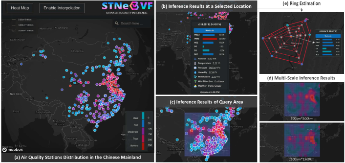
Nonetheless, the deployment of air quality stations within urban environments is usually scarce (see Figure 2(a)), hindered by the prohibitively high costs associated with station establishment and maintenance. Specifically, the establishment of a station necessitates a huge land footprint, entailing a non-trivial financial investment, around 200,000 USD for construction and an annual maintenance cost of 30,000 USD Zheng et al. (2013). The sustained operation also requires dedicated human resources for routine upkeep. This resource-intensive nature of traditional monitoring stations exacerbates the scarcity of these installations in urban landscapes.
In the past decade, substantial research endeavors have been directed towards air quality inference Han et al. (2023), seeking to infer real-time air quality in locations devoid of monitoring stations by leveraging data gleaned from existing sites, as shown in Figure 2(b)-(c). Traditional methods Hasenfratz et al. (2014); Jumaah et al. (2019) rely on linear spatial assumptions, but this approach falls short due to non-linear variations influenced by factors like meteorology, traffic, population density, and land use, which constrain the effectiveness in capturing the complexities of air quality data. With recent advancements in deep learning, Graph Neural Networks (GNN) Kipf and Welling (2016a) have become dominant for non-Euclidean data representation, particularly in learning complex spatial correlations among air quality monitoring stations. Integrating GNNs with temporal learning modules(e.g., RNN Graves (2013), TCN Bai et al. (2018)) has led to the development of Spatio-Temporal Graph Neural Networks (STGNN)Wang et al. (2020); Jin et al. (2023), addressing the dynamic nature of air quality data across spatial and temporal dimension. STGNNs, exemplified in studies like Han et al. (2021); Hu et al. (2023b) offer superior representation extraction and flexibility in cross-domain data fusion.
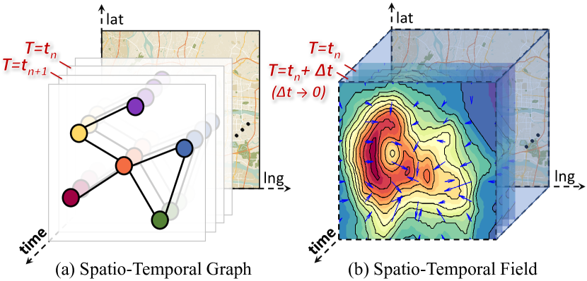
Though promising, STGNNs simply treat air quality data as a Spatio-Temporal Graph (STG), as shown in Figure 1(a). However, these models overlook a crucial property – continuity, which manifests across both spatial and temporal dimensions. In reality, air quality readings of stations are sampled from a continuous Euclidean space and cannot be fully encapsulated by a discrete graph structure using GNNs. Meanwhile, the temporal modules (e.g., RNN, TCN) in STGNNs exhibit the discrete nature as well, rendering them incapable of capturing continuous-time dynamics within data. To better represent the continuous and evolving nature of real-world air quality phenomena, a more powerful approach is needed, surpassing the discrete representation of STGNNs.
In this paper, we draw inspiration from Field Theory McMullin (2002) and innovatively formulate air quality inference from a field perspective, where air quality data is a physical quantity that can be conceptualized by a new concept called Spatio-Temporal Fields (STF), as depicted in Figure 1(b). These fields encompass three dimensions (i.e., latitude, longitude, time), assigning a distinct value to each point in spacetime. In contrast to STGs, STFs are characterized by being regular, continuous, and unified111It implies that the field representation accounts for variations not only across different locations in space but also over different points in time, emphasizing the comprehensive treatment of both spatial and temporal aspects within the unified framework., offering a representation more aligned with reality. Under this perspective, we can transform the air quality inference problem to reconstruct STFs from available readings using coordinate-based neural networks, particularly Implicit Neural Representations (INR) Sitzmann et al. (2020); Xie et al. (2022).
While INRs effectively handle the continuity property of air quality data, they inevitably confront two primary challenges. Firstly, the generation process of air quality data is extremely complex and influenced by various factors (such as humidity and wind speed/direction), which poses a challenge for reconstructing the underlying STFs through neural representation methods. Secondly, empirical studies Xu et al. (2019); Sitzmann et al. (2020) verify that INRs always exhibit a bias towards learning low-frequency functions, which will disregard locally varying high-frequency information and higher-order derivatives even with dense supervision.
To this end, we for the first time present Spatio-Temporal Field Neural Networks (STFNN), opening new avenues for modeling spatio-temporal fields and achieving state-of-the-art performance in nationwide air quality inference in the Chinese Mainland. Targeting the first challenge, we pivot our focus from reconstructing the value of each entry in STFs to learning the derivative (i.e., gradient) of each entry. This strategic shift is inspired by learning the residual is often easier than learning the original value directly, as exemplified in ResNet He et al. (2016). Such vector field can not only show how the pollutant concentration varies across time and space but also the direction of diffusion. To tackle the second challenge, we endeavor to augment our STFNN with local context knowledge during air quality inference at a specific location. Specifically, we combine the STGNN’s capability to capture local spatio-temporal dependencies with STFNN’s ability to learn global spaito-temporal unified representations. This integration results in what we term Pyramid Inference, a hybrid framework that leverages the strengths of both models to achieve a more comprehensive inference of air quality dynamics with both high-frequency and low-frequency components. Overall, our contributions lie in three aspects:
-
•
A Field Perspective. We formulate air quality as spatio-temporal fields with the first shot. Compared to STGs, our STFs not only adeptly capture the continuity and Euclidean structure of air quality data, but also achieves a unified representation across both space and time.
-
•
Spatio-Temporal Field Neural Networks. We propose a groundbreaking network called STFNN to model STF data. STFNN pioneers an implicit representation of the STF’s gradient, deviating from conventional direct estimation approaches. Moreover, it preserves high-frequency information via Pyramid Inference.
-
•
Empirical Evidence. We conduct extensive experiments to evaluate the effectiveness of our STFNN. The results valiadte that STFNN outperforms prior arts by a significant margin and exhibits compelling properties. A system in Figure 2 has been deployed to show its practicality in the Chinese Mainland.
2 Preliminary
Definition 1 Air Quality Reading We use and to denote the air quality readings and the concentration of PM2.5, which is the most important air pollutant, from the -th monitoring stations at time separately. Here encompasses various measurements, such as concentrations of other air pollutants (e.g., PM10, \chemfigNO_2), and meteorological properties (e.g. humidity, weather and wind speed). denotes the observations of all stations at a specified time . denotes the observations of all stations at all time. Similar definitions apply to and , mirroring and , respectively.
Definition 2 (Coordinates) A coordinate is used to represent the spatial and temporal properties of an air quality reading or a location, including longitude, latitude, and timestamp. These coordinates are categorized into two types: source coordinate , associated with readings or locations with existing air quality monitoring stations, while target coordinate , corresponding to unobserved locations requiring inference. Notably, represents the coordinate of the corresponding and . Parallel definitions apply to and in relation to and , respectively, which are not reiterated here.
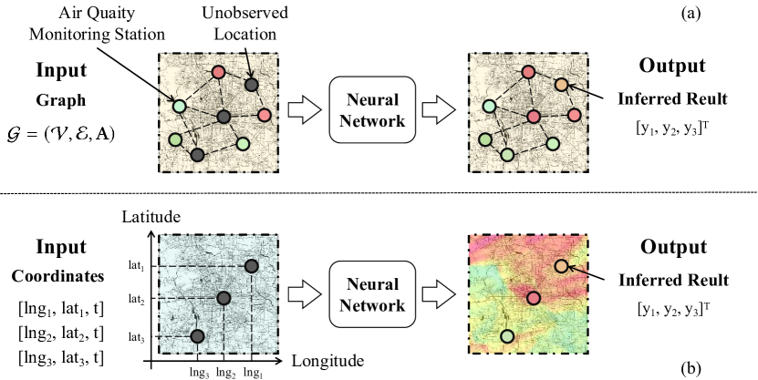
Problem Definition The air quality inference problem addresses the utilization of historical data and real-time readings from a limited number of air quality monitoring stations to infer the real-time air quality anywhere (especially unobserved location). The conventional strategies Hou et al. (2022); Hu et al. (2023a) involve designating the location to be inferred as the masked node and constructing a graph to capture relationships between stations and locations, as shown in Figure 3 (a). The task is then framed as a node recovery problem, focusing on restoring the masked nodes. In this paper, we revisit the problem from the field perspective, as shown in Figure 3 (b). Specifically, our goal is to reconstruct a spatio-temporal field for air quality that is capable of mapping any arbitrary coordinate, especially , to the corresponding concentration of PM2.5 , which can be formulated as
| (1) |
Additional parameters, such as , are allowed to enhance the inference process.
3 Methodology
In this section, we elucidate fundamental concepts underlying two distinct spacetime perspectives: the Spatio-Temporal Field and the Spatio-Temporal Graph. Subsequently, we integrate these perspectives to formulate our proposed hybrid framework, the Pyramidal Inference.
3.1 Global View: Spatio-Temporal Field
A Spatio-Temporal Field (STF) is a global modeling of air quality that encompasses all stations and observation times. The STF function, denoted as , assigns a unique physical quantity to each coordinate. When is a scalar, represents a scalar field. Conversely, if is a vector, with magnitude and direction, it denotes a vector field.
Specifically, our focus lies on a scalar field for air quality inference, where maps the coordinates to the corresponding PM2.5 concentration. This representation facilitates a continuous and unified spacetime perspective, allowing for the inference of air quality at any location and time by inputting the coordinates.
Directly modeling is challenging due to its intricate complexity and nonlinearity. Alternatively, it is often more feasible to learn its derivative, which refers to the gradient field of in spacetime. We denote the gradient field as which is a vector field. Notably, given a specific , an array of solutions exists unless an initial value is specified. We use and to denote the PM2.5 concentration on and , respectively. Our primary focus lies in inferring since the true value of is known and recorded, while remains undisclosed. To infer , we utilize a as the initial value and assume is a piecewise smooth curve in that point from to , then we have
| (2) |
where is the dot product, and represents the position vector, serving as a bijective parametrization of the curve . The endpoints of are given by and , with . Seeking an Implicit Neural Representation (INR) becomes the objective to fit as is usually intricate to the extent that it cannot be explicitly formulated. More details are introduced in the Appendix B.
3.2 Local View: Spatio-Temporal Graph
The formulation presented in Eq. (2) ensures the recoverability of across arbitrary coordinates through curve integration, utilizing solely a single initial value. However, this approach yields an excessively coarse representation of the entire STF, resulting in the loss of numerous local details and high-frequency components, thereby introducing significant errors. The impact is particularly pronounced when is situated at a considerable distance from as the increase in the length of introduces a significant cumulative error.
In response to this limitation, we leverage the potent learning capabilities of STGNN to capture local spatio-temporal correlations effectively. Building upon the foundational workSong et al. (2020), we employ the local spatio-temporal graph (STG) to model the spatio-temporal dependencies of the given coordinates and their neighboring air monitoring stations with their histories. To avoid trivializing the description, we put the details in Appendix C.
3.3 Hybrid Framework: Pyramidal Inference
We intend to integrate the continuous and uniform global modeling of spacetime provided by STF with the local detailing capabilities of STG, thereby establishing a hybrid framework that leverages the strengths of both approaches. Within the local STG, the estimation of is achieved by leveraging information from its neighboring nodes through Eq. (2). By calculating estimates of from these neighbors and assigning a learnable weight to each estimation (), we enhance the precision of the inference result for a specific coordinate. This operation can be formulated as
| (3) |
where is the joint estimation of by neighbors. and represent the weight and PM2.5 concentration of the neighbor, respectively. is the integral path in that points from the coordinates of the neighbor to the target coordinate.
We call the inference strategy represented by Eq. (3) Pyramidal Inference, which is the framework of the STFNN we propose. To demonstrate its sophistication, we deconstruct Eq. (3) into two steps:
| (4) |
and
| (5) |
where is the estimate of by the neighbor, and represent the vector form of and , respectively. These two operations can be viewed as follows. In Eq. (4), a curve integral is used over the gradient field to estimate from each neighbor in a continuous and spatio-temporally uniform way, which takes advantage of the STF. In Eq. (5), the information from the neighbors is aggregated through , which considers the spatio-temporal dependencies between the nodes and takes advantage of the STG. In this way, the Pyramidal Inference framework combines the two different spacetime perspectives into a distinctive new paradigm.
4 IMPLEMENTATION
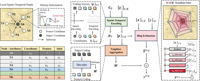
Upon introducing the formulation of Pyramidal Inference, we proceed to its implementation through a meticulously designed model architecture, depicted in Figure 4. The model comprises three pivotal components:
-
•
Spatio-Temporal Encoding. This component transforms coordinates into coded vectors endowed with representational meaning, enhancing the network’s ability to comprehend and leverage the spatio-temporal characteristics of coordinates.
-
•
Ring Estimation: Implementation of Eq. (4), mapping the encoded vector to the gradient of the STF. This process yields each neighbor’s estimate of the PM2.5 concentration for the target coordinates through a path integral.
-
•
Neighbor Aggregation: Implementation of Eq. (5), utilizing the coded vectors of neighbors and target coordinates as inputs to derive the estimated weights for each neighbor concerning the target coordinates.
In the following parts, we will provide a detailed exposition of each module, elucidating their functionalities step by step.
4.1 Spatio-Temporal Encoding
We revisit the previously introduced local STG, which amalgamates nodes across different time steps into a unified graph, potentially obscuring the inherent temporal properties of individual nodes. In essence, this local STG places nodes from diverse time steps into a shared environment without discerning their temporal distinctions. However, This issue can be mitigated through meticulous positional coding of nodesGehring et al. (2017); Song et al. (2020).
We use to denote the coding vector, essential for accurately describing the spatio-temporal characteristics of a node or coordinate. This vector is expressed as the concatenation , where represents spatial coding and represents temporal coding. In the spatial dimension, a node’s properties can be captured by its absolute position, represented by z-normalized longitude and latitude , forming . For encoding temporal information , sinusoidal functions with different periods are employed, reflecting the periodic nature of temporal phenomena. We utilize a set of periods , with as the scaling index, to represent days, weeks, months, and years. The temporal coding is then represented as:
| (6) |
where denotes the value of the dimension () of , denotes dividing by 2 and rounding down, and is the period of . Consequently, comprises a two-dimensional spatial code and an eight-dimensional temporal code .
4.2 Ring Estimation
Motivation. We employ the continuous approach of curve integration over the gradient to determine the PM2.5 concentration at the target coordinate in Eq. (4). However, due to inherent limitations in numerical accuracy within computing systems, achieving true continuity in STF becomes unattainable. Therefore, we have adopted an incremental approach. We set the integral path to be a straight line from the neighbors’ coordinate to the target coordinate for convenience, then the unit direction vector in the path can be written as . After that, we replace the integral operation with a summation operation and modify Eq. (4) to a discrete form
| (7) |
where represents the step size of the summation and is the coordinate of the node in the local STG. represents the difference at the step of the node, which is the discrete approximation of the gradient. Our objective is to build a module for estimating , which is the only unknown in Eq. (7).
Overview. Towards this objective, we introduce a pivotal module named Ring Estimation, designed for the joint estimation of the differences at the step of all neighbors. We posit that simultaneous estimation of enhances inference efficiency and captures correlations between them, thereby reducing estimation errors compared to individually estimating for a single neighbor times. Specifically, the Ring Estimation module divides the polygon surrounded by neighbors around the target coordinate into ring zones from the outermost to the innermost, with total of transition nodes (coordinates) uniformly spaced along the inference path. The inner edge of the ring zone serves as the outer edge for the zone. Like the target coordinate, the transition nodes lack features and labels (PM2.5 concentration). They serve as the intermediary states and springboards in the process of estimating . By increasing the value of , the Ring Estimation block facilitates the inference in an approximately continuous manner. In consideration of space constraints, the implementation details of Ring Estimation are provided in the Appendix E.1.
4.3 Neighbor Aggregation.
It is advisable to assign varying weights to the estimations of the target nodes based on the different spatio-temporal scenarios in which they are situated. To this end, we present the Neighbor Aggregation module, which takes into account the coding of the coordinates of the neighbors and the target coordinate and employs end-to-end learning to compute the estimation weights of each neighbor on the target node. The Transformer-Decoder structure mentioned in Appendix D and E.1 is still being followed due to its numerous benefits. Due to space constraints, a comprehensive elaboration of Neighbor Aggregation is provided in Appendix E.2.
5 Experiments
In this section, we delve into our experimental methodology aimed at evaluating the performance and validating the efficacy of the STFNN. We present a detailed account of the experimental setup, data collection procedures, evaluation metrics, and results obtained, aiming to demonstrate the performance, robustness, and scalability of our approach. Specifically, our experiments are designed to explore the following research questions, elucidating key aspects of our approach and its applicability in real-world scenarios:
-
•
RQ1: How does STFNN’s approach, focusing on inferring concentration gradients for indirect concentration value prediction, outperform traditional methods in terms of accuracy and effectiveness?
-
•
RQ2: What specific contributions do the individual components of STFNN make to its effectiveness in predicting air pollutant concentrations?
-
•
RQ3: How do variations in each hyperparameter impact the overall performance of STFNN?
-
•
RQ4: Do the three-dimensional hidden states learned by the model accurately represents the gradient of the spatio-temporal field?
-
•
RQ5: Can our model demonstrate proficient performance in inferring concentrations of various air pollutants, including \chemfigNO_2?
Due to the page limit, more details about the experiments are provided in the Appendix F.
5.1 Experimental Settings
5.1.1 Datasets
Our study procured a nationwide air quality datasetLiang et al. (2023) spanning a comprehensive temporal scope from January 1st, 2018, to December 31st, 2018. The spatial distribution of monitoring stations is shown in Figure 2(a), demonstrating extensive coverage that exceeds previous datasets in scale and breadth. This dataset not only includes air quality data but also meteorological data. The input data can be divided into two classes: continuous and categorical data. Continuous data include critical parameters such as air pollutant concentrations (e.g., PM2.5, CO), temperature, wind speed, and others. Categorical data include variables such as weather conditions, wind direction, and time indicators. In the face of unforeseen circumstances, such as force majeure events or operational disruptions (e.g., power outages, monitoring station maintenance), certain data instances have missing values.
5.2 Model Comparison (RQ1)
In addressing RQ1, we conduct a meticulous comparative analysis among models based on the evaluation metrics of MAE, RMSE, and MAPE. The empirical outcomes derived from this analysis are systematically presented across the expansive spectrum of the nationwide air quality dataset, meticulously documented within Table 1.
| Model | Year | #Param(M) | Mask Ratio = 25% | Mask Ratio = 50% | Mask Ratio = 75% | |||||||||
|---|---|---|---|---|---|---|---|---|---|---|---|---|---|---|
| MAE | RMSE | MAPE | MAE | RMSE | MAPE | MAE | RMSE | MAPE | ||||||
| KNN | 1967 | - - | 30.50 | +146.0% | 65.40 | 1.36 | 30.25 | +145.5% | 72.23 | 0.71 | 34.07 | +194.0% | 74.55 | 0.64 |
| RF | 2001 | 29.22 | +135.6% | 68.95 | 0.76 | 29.71 | +141.2% | 71.61 | 0.75 | 29.82 | +157.3% | 70.99 | 0.74 | |
| MCAM | 2021 | 0.408 | 23.94 | +93.1% | 36.25 | 0.95 | 25.01 | +103.0% | 37.94 | 0.92 | 25.19 | +117.3% | 37.82 | 1.04 |
| SGNP | 2019 | 0.114 0.108 | 23.60 | +90.3% | 37.58 | 0.83 | 24.06 | +95.3% | 37.08 | 0.93 | 21.68 | +87.1% | 33.68 | 0.84 |
| STGNP | 2022 | 23.21 | +87.2% | 38.13 | 0.62 | 21.95 | +78.2% | 37.13 | 0.67 | 19.58 | +68.9% | 31.95 | 0.69 | |
| VAE | 2013 | 0.011 0.073 0.073 | 28.49 | +129.8% | 67.11 | 0.94 | 28.92 | +134.7% | 69.67 | 0.94 | 29.00 | +150.2% | 69.11 | 0.93 |
| GAE | 2016 | 12.63 | +1.9% | 23.80 | 0.46 | 12.78 | +3.7% | 24.11 | 0.46 | 12.57 | +8.5% | 23.73 | 0.46 | |
| GraphMAE | 2022 | 12.40 | - | 23.20 | 0.46 | 12.32 | - | 23.11 | 0.46 | 11.59 | - | 21.51 | 0.43 | |
| STFNN | - | 0.208 | 11.14 | -10.2% | 19.75 | 0.23 | 11.32 | -8.1% | 19.91 | 0.24 | 11.27 | -2.8% | 19.86 | 0.24 |
The results indicate that STFNN consistently demonstrates enhanced efficacy across various evaluation metrics, surpassing existing baseline models. Table 1 shows that our approach reduces MAE under three different mask ratios (25%, 50%, and 75%) in comparison to GraphMAE, establishing a new State-of-the-Art (SOTA) in nationwide PM2.5 concentration inference in the Chinese Mainland. In our view, there are two main reasons for this. Firstly, the adoption of the gradient field as a more intrinsic representation enhances the network’s ability to learn the inherent dynamical processes of spatial and temporal evolution, aligning more closely with the reality of physical quantities. Secondly, the unified and continuous nature of STFNN’s spatial and temporal modules enables simultaneous capture of both types of information, avoiding bias or information loss inherent in separate delivery. Lastly, the Pyramidal Inference framework we proposed adeptly captures global and local spatio-temporal properties, facilitating more accurate modeling of the pollutant concentration field.
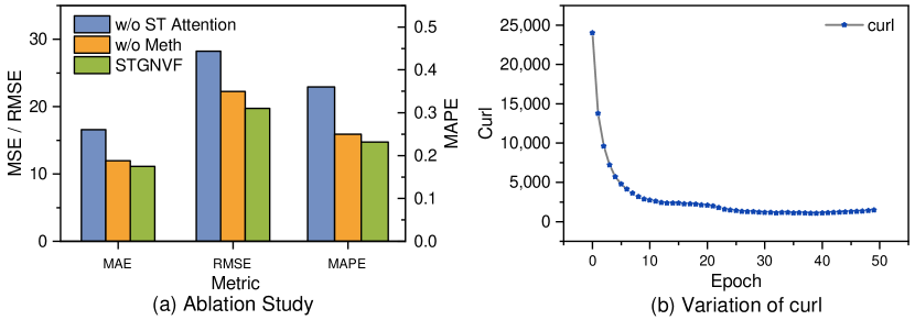
5.3 Ablation Study (RQ2)
To assess the contributions of individual components to the performance of our model and address RQ2, we conducted ablation studies. The findings from these studies are presented in Figure 5 (a). Each study involved modifying only the relevant component while keeping other settings constant.
Effects of meteorological features. To analyze the impact of meteorological features on the accuracy of the final model, we removed them from the raw data. Therefore, the gradient was obtained solely from the spatio-temporal coordinates of neighboring stations fed into the gradient encoder. The figure demonstrates that removing the meteorological features resulted in some improvement in the model’s mean absolute error (MAE), which still outperformed all baseline models. This phenomenon demonstrates that STFNN’s learning capability is powerful enough to restore the entire STF through the scalar’s information, which shows the superiority of our proposed framework.
Effects of Neighbor Aggregation. To investigate the impact of a dynamic and learnable implicit graph structure on the model, we substituted the model’s Neighbor Aggregation module with IDW and SES, a non-parametric approach inspired by Zheng et alZheng et al. (2013). This approach employs implicit graph relations that are static. The results depicted in Figure 5 (a) demonstrate that utilizing the Neighbor Aggregation module results in a significant decrease in MAE.
5.4 Hyperparameters Study (RQ3)
In this section, we comprehensively explore the effects of various hyperparameters on the model’s performance, thereby addressing RQ3.
Effects of Hidden & FFD Dimension. We adjusted the hidden layer dimension of the Spatio-Temporal Encoding module and the forward propagation of the Transformer-Decoder structure used by the Ring Estimation and Neighbor Aggregation modules from 16 to 64. The results in Figure 6 (a-b) show that adjusting the hidden layer dimension has little effect on the absolute values of MAE and RMSE, but it significantly decreases MAPE. This improvement is mainly due to the small value of the air pollutant concentration itself.
Effects of Step Size. We vary the value of the accumulation step size of the Ring Estimation in . The result is shown in Figure 6 (c). It has been observed that as the step size increases, the model’s performance initially declines before improving. Additionally, when comparing 2 steps to 16 steps, we note that the model’s training time per round is approximately 50% longer for 16 steps. However, this increase in step size enables us to obtain a more precise gradient at each point on the integration path, resulting in a more intricate representation of the spatio-temporal field.
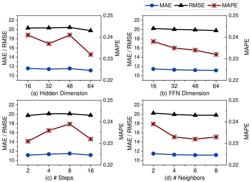
Effects of Neighbors Number. We vary the number of neighbors from 2 to 8, and the result is shown in Figure 6 (d). We observe that the performance of our model improved as the number of neighbors increased. Notably, our proposed STFNN exhibited excellent performance even with a small number of neighbors. Due to its ability to learn global spatio-temporal patterns, the model can use global information for inference even in scenarios where there are only a few neighbors present. When the number of neighbors increases, STFNN can utilize local information for inference, resulting in reduced error.
5.5 Interpretability (RQ4)
To confirm that the network’s learned vector is the gradient of the spatio-temporal field, we calculate the curl variation with the number of training epochs. We use Yang et al.’s methodYang et al. (2023) to quantify the curl and present the experimental results in Figure 5 (b). It is evident that the curl of the vector field obtained by the network decreases as the training progresses, indicating successful learning of the gradient field.
5.6 Generalizability (RQ5)
Our model not only excels in predicting PM2.5 but also establishes a new benchmark, achieving the SOTA in inferring the concentration of \chemfigNO_2, as shown in Table 2. This noteworthy outcome underscores the versatility of our model across distinct air quality parameters. In comparison to the baseline, our model demonstrates a significant advantage, showcasing its capability to handle diverse pollutants effectively and outperforming established methods in inference for \chemfigNO_2.
| Model | Mask Ratio = 25% | Mask Ratio = 50% | Mask Ratio = 75% | |||
|---|---|---|---|---|---|---|
| MAE | RMSE | MAE | RMSE | MAE | RMSE | |
| KNN | 18.10 | 62.51 | 18.47 | 64.22 | 20.18 | 62.86 |
| RF | 16.90 | 61.25 | 17.60 | 64.91 | 17.36 | 63.70 |
| MCAM | 18.25 | 27.80 | 17.75 | 27.42 | 21.17 | 29.41 |
| SGNP | 17.66 | 25.43 | 19.17 | 26.36 | 16.57 | 24.11 |
| STGNP | 16.43 | 27.85 | 15.62 | 26.06 | 15.70 | 26.23 |
| VAE | 29.85 | 112.81 | 31.43 | 119.59 | 30.82 | 117.33 |
| GAE | 12.80 | 30.16 | 12.77 | 30.16 | 12.77 | 30.00 |
| GraphMAE | 12.76 | 30.25 | 12.60 | 29.53 | 12.48 | 29.30 |
| STFNN | 11.34 | 23.65 | 11.52 | 24.93 | 11.97 | 25.81 |
6 Conclusion
In this work, we introduced a novel perspective for air quality inference, framing it as a problem of reconstructing Spatio-Temporal Fields (STFs) to better capture the continuous and unified nature of air quality data. Our proposed Spatio-Temporal Field Neural Network (STFNN) breaks away from the limitations of Spatio-Temporal Graph Neural Networks (STGNNs) by focusing on implicit representations of gradients, offering a more faithful representation of the dynamic evolution of air quality phenomena. As we exploring the intricate dynamics of air quality, this work sets the stage for further advancements in environmental monitoring and predictive modeling.
References
- Ba et al. [2016] Jimmy Lei Ba, Jamie Ryan Kiros, and Geoffrey E Hinton. Layer normalization. arXiv preprint arXiv:1607.06450, 2016.
- Bai et al. [2018] Shaojie Bai, J Zico Kolter, and Vladlen Koltun. An empirical evaluation of generic convolutional and recurrent networks for sequence modeling. arXiv preprint arXiv:1803.01271, 2018.
- Bai et al. [2020] Lei Bai, Lina Yao, Can Li, Xianzhi Wang, and Can Wang. Adaptive graph convolutional recurrent network for traffic forecasting. Advances in neural information processing systems, 33:17804–17815, 2020.
- Cheng et al. [2018] Weiyu Cheng, Yanyan Shen, Yanmin Zhu, and Linpeng Huang. A neural attention model for urban air quality inference: Learning the weights of monitoring stations. In Proceedings of the AAAI conference on artificial intelligence, volume 32, 2018.
- Fawagreh et al. [2014] Khaled Fawagreh, Mohamed Medhat Gaber, and Eyad Elyan. Random forests: from early developments to recent advancements. Systems Science & Control Engineering: An Open Access Journal, 2(1):602–609, 2014.
- Gehring et al. [2017] Jonas Gehring, Michael Auli, David Grangier, Denis Yarats, and Yann N Dauphin. Convolutional sequence to sequence learning. In International conference on machine learning, pages 1243–1252. PMLR, 2017.
- Geng et al. [2019] Xu Geng, Yaguang Li, Leye Wang, Lingyu Zhang, Qiang Yang, Jieping Ye, and Yan Liu. Spatiotemporal multi-graph convolution network for ride-hailing demand forecasting. In Proceedings of the AAAI conference on artificial intelligence, volume 33, pages 3656–3663, 2019.
- Graves [2013] Alex Graves. Generating sequences with recurrent neural networks. arXiv preprint arXiv:1308.0850, 2013.
- Guo et al. [2003] Gongde Guo, Hui Wang, David Bell, Yaxin Bi, and Kieran Greer. Knn model-based approach in classification. In On The Move to Meaningful Internet Systems 2003: CoopIS, DOA, and ODBASE: OTM Confederated International Conferences, CoopIS, DOA, and ODBASE 2003, Catania, Sicily, Italy, November 3-7, 2003. Proceedings, pages 986–996. Springer, 2003.
- Han et al. [2021] Qilong Han, Dan Lu, and Rui Chen. Fine-grained air quality inference via multi-channel attention model. In IJCAI, pages 2512–2518, 2021.
- Han et al. [2023] Jindong Han, Weijia Zhang, Hao Liu, and Hui Xiong. Machine learning for urban air quality analytics: A survey. arXiv preprint arXiv:2310.09620, 2023.
- Hasenfratz et al. [2014] David Hasenfratz, Olga Saukh, Christoph Walser, Christoph Hueglin, Martin Fierz, and Lothar Thiele. Pushing the spatio-temporal resolution limit of urban air pollution maps. In 2014 IEEE International Conference on Pervasive Computing and Communications (PerCom), pages 69–77. IEEE, 2014.
- He et al. [2016] Kaiming He, Xiangyu Zhang, Shaoqing Ren, and Jian Sun. Deep residual learning for image recognition. In Proceedings of the IEEE conference on computer vision and pattern recognition, pages 770–778, 2016.
- Hou et al. [2022] Zhenyu Hou, Xiao Liu, Yukuo Cen, Yuxiao Dong, Hongxia Yang, Chunjie Wang, and Jie Tang. Graphmae: Self-supervised masked graph autoencoders, 2022.
- Hu et al. [2023a] Junfeng Hu, Yuxuan Liang, Zhencheng Fan, Hongyang Chen, Yu Zheng, and Roger Zimmermann. Graph neural processes for spatio-temporal extrapolation. arXiv preprint arXiv:2305.18719, 2023.
- Hu et al. [2023b] Junfeng Hu, Yuxuan Liang, Zhencheng Fan, Li Liu, Yifang Yin, and Roger Zimmermann. Decoupling long-and short-term patterns in spatiotemporal inference. IEEE Transactions on Neural Networks and Learning Systems, 2023.
- Jiang et al. [2021] Renhe Jiang, Du Yin, Zhaonan Wang, Yizhuo Wang, Jiewen Deng, Hangchen Liu, Zekun Cai, Jinliang Deng, Xuan Song, and Ryosuke Shibasaki. Dl-traff: Survey and benchmark of deep learning models for urban traffic prediction. In Proceedings of the 30th ACM international conference on information & knowledge management, pages 4515–4525, 2021.
- Jin et al. [2023] Guangyin Jin, Yuxuan Liang, Yuchen Fang, Jincai Huang, Junbo Zhang, and Yu Zheng. Spatio-temporal graph neural networks for predictive learning in urban computing: A survey. arXiv preprint arXiv:2303.14483, 2023.
- Jumaah et al. [2019] Huda Jamal Jumaah, Mohammed Hashim Ameen, Bahareh Kalantar, Hossein Mojaddadi Rizeei, and Sarah Jamal Jumaah. Air quality index prediction using idw geostatistical technique and ols-based gis technique in kuala lumpur, malaysia. Geomatics, Natural Hazards and Risk, 10(1):2185–2199, 2019.
- Kingma and Welling [2022] Diederik P Kingma and Max Welling. Auto-encoding variational bayes, 2022.
- Kipf and Welling [2016a] Thomas N Kipf and Max Welling. Semi-supervised classification with graph convolutional networks. arXiv preprint arXiv:1609.02907, 2016.
- Kipf and Welling [2016b] Thomas N. Kipf and Max Welling. Variational graph auto-encoders, 2016.
- Li et al. [2017] Yaguang Li, Rose Yu, Cyrus Shahabi, and Yan Liu. Diffusion convolutional recurrent neural network: Data-driven traffic forecasting. arXiv preprint arXiv:1707.01926, 2017.
- Liang et al. [2023] Yuxuan Liang, Yutong Xia, Songyu Ke, Yiwei Wang, Qingsong Wen, Junbo Zhang, Yu Zheng, and Roger Zimmermann. Airformer: Predicting nationwide air quality in china with transformers. In Proceedings of the AAAI Conference on Artificial Intelligence, volume 37, pages 14329–14337, 2023.
- McMullin [2002] Ernan McMullin. The origins of the field concept in physics. Physics in Perspective, 4:13–39, 2002.
- Salim and Haque [2015] Flora Salim and Usman Haque. Urban computing in the wild: A survey on large scale participation and citizen engagement with ubiquitous computing, cyber physical systems, and internet of things. International Journal of Human-Computer Studies, 81:31–48, 2015.
- Singh et al. [2019] Gautam Singh, Jaesik Yoon, Youngsung Son, and Sungjin Ahn. Sequential neural processes, 2019.
- Sitzmann et al. [2020] Vincent Sitzmann, Julien Martel, Alexander Bergman, David Lindell, and Gordon Wetzstein. Implicit neural representations with periodic activation functions. Advances in neural information processing systems, 33:7462–7473, 2020.
- Song et al. [2020] Chao Song, Youfang Lin, Shengnan Guo, and Huaiyu Wan. Spatial-temporal synchronous graph convolutional networks: A new framework for spatial-temporal network data forecasting. In Proceedings of the AAAI conference on artificial intelligence, volume 34, pages 914–921, 2020.
- Sun et al. [2020] Junkai Sun, Junbo Zhang, Qiaofei Li, Xiuwen Yi, Yuxuan Liang, and Yu Zheng. Predicting citywide crowd flows in irregular regions using multi-view graph convolutional networks. IEEE Transactions on Knowledge and Data Engineering, 34(5):2348–2359, 2020.
- Vallero [2014] Daniel A Vallero. Fundamentals of air pollution. Academic press, 2014.
- Vaswani et al. [2017] Ashish Vaswani, Noam Shazeer, Niki Parmar, Jakob Uszkoreit, Llion Jones, Aidan N Gomez, Łukasz Kaiser, and Illia Polosukhin. Attention is all you need. Advances in neural information processing systems, 30, 2017.
- Wang et al. [2020] Senzhang Wang, Jiannong Cao, and S Yu Philip. Deep learning for spatio-temporal data mining: A survey. IEEE transactions on knowledge and data engineering, 34(8):3681–3700, 2020.
- Wang et al. [2021] Huandong Wang, Qiaohong Yu, Yu Liu, Depeng Jin, and Yong Li. Spatio-temporal urban knowledge graph enabled mobility prediction. Proceedings of the ACM on interactive, mobile, wearable and ubiquitous technologies, 5(4):1–24, 2021.
- Wu et al. [2019] Zonghan Wu, Shirui Pan, Guodong Long, Jing Jiang, and Chengqi Zhang. Graph wavenet for deep spatial-temporal graph modeling. arXiv preprint arXiv:1906.00121, 2019.
- Xie et al. [2022] Yiheng Xie, Towaki Takikawa, Shunsuke Saito, Or Litany, Shiqin Yan, Numair Khan, Federico Tombari, James Tompkin, Vincent Sitzmann, and Srinath Sridhar. Neural fields in visual computing and beyond. In Computer Graphics Forum, volume 41, pages 641–676. Wiley Online Library, 2022.
- Xu et al. [2019] Zhi-Qin John Xu, Yaoyu Zhang, Tao Luo, Yanyang Xiao, and Zheng Ma. Frequency principle: Fourier analysis sheds light on deep neural networks. arXiv preprint arXiv:1901.06523, 2019.
- Yang et al. [2023] Xianghui Yang, Guosheng Lin, Zhenghao Chen, and Luping Zhou. Neural vector fields: Generalizing distance vector fields by codebooks and zero-curl regularization. arXiv preprint arXiv:2309.01512, 2023.
- Yu et al. [2017] Bing Yu, Haoteng Yin, and Zhanxing Zhu. Spatio-temporal graph convolutional networks: A deep learning framework for traffic forecasting. arXiv preprint arXiv:1709.04875, 2017.
- Zheng et al. [2013] Yu Zheng, Furui Liu, and Hsun-Ping Hsieh. U-air: When urban air quality inference meets big data. In Proceedings of the 19th ACM SIGKDD international conference on Knowledge discovery and data mining, pages 1436–1444, 2013.
Appendix A Related Works
A.1 Air Quality Inference
Air quality inference is a task that involves inferring the air quality value of a target area based on known information. Previous studies used statistical machine learning methods, such as K-Nearest Neighbors (KNN) and Random Forest (RF) Fawagreh et al. [2014], to tackle this problem. KNN techniques rely on linear relationships between data points, while RF can understand non-linear relationships. However, these models only consider simple spatial relationships and do not adapt to complex changes in air quality. Recently, Neural Networks(NNs) have become the leading approach. The attention mechanism is introduced to integrate the features of sensors Cheng et al. [2018]; Han et al. [2021]. This enhances the model to accurately understand and use data from multiple sources over temporal and spatial. However, these NNs can overfit on datasets with limited data and may fail to accurately represent complex, non-linear interactions between various air pollutants and external factors. On the contrary, our model is capable of accomplishing both objectives.
A.2 Spatio-Temporal Graph Neural Networks
In recent times, there’s been a growing interest in studying Spatio-Temporal Graphs (STGs) to understand the intricate relationship that involves both spatial and temporal. STGNNsJiang et al. [2021]; Salim and Haque [2015]; Wang et al. [2020]; Sun et al. [2020]; Wang et al. [2021], which integrate the strengths of GNNs, have emerged as the leading approach for uncovering intricate relationships in STG data. Some follow-ups Li et al. [2017]; Yu et al. [2017]; Geng et al. [2019] introduce temporal components such as Recurrent Neural Networks (RNN) Graves [2013] and Temporal Convolutional Networks (TCN) Bai et al. [2018] to better address the spatio-temporal dependencies. Recent progress in this area includes the development of Graph WaveNet Wu et al. [2019] and AGCRN Bai et al. [2020], which use adaptive adjacency matrices to improve their performance. Variants incorporating self-attention mechanisms Vaswani et al. [2017] adaptively capture dynamic spatio-temporal dependencies within air quality data, enhancing predictive performance Liang et al. [2023]. However, The limitation of STGNNs lies in their lack of consideration for contiguity and Euclidean spatial structures, which is inconsistent with the actual essence of air diffusion.
Appendix B Curl of the Gradient Field
Importantly, the recovered gradients possess real physical significance, manifesting in special properties such as a constant zero-curl, which can be formulated as
| (8) |
and it will be theoretically proven in the following:
Theorem 1.
Proof.
Let be a scalar-valued function. Then its gradient
| (9) |
is a vector field, which we denote by . We can easily calculate that the curl of is zero. We use the formula for curl in terms of its components
| (10) |
Since each components of is a derivative of , we can rewrite the curl as
| (11) |
If is twice continuously differentiable, then its second derivatives are independent of the order in which the derivatives are applied. All the terms cancel in the expression for curl , and we conclude that curl . ∎
Additionally, we have experimentally demonstrated it in Section 5.5. This property holds substantial importance in accurately characterizing the three-dimensional vectors representing the STF’s gradient, enhancing the overall interpretability of our model.
Another way to express Equation (8) is that is conservative, which means that the result of the curve integration is only dependent on the start and end points of the integration path, and not on the shape of the path itself. For convenience, we set to be a straight line from the start to the end.
Appendix C Local Spatio-Temporal Graph
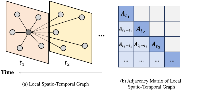
To achieve the local STG, during each time within the past period , we consider coordinates and their nearest stations as nodes. By using edges to connect stations and their previous moments with the coordinate, we can get the local STG, which we denote as , where is the node set, is the edge set and is the adjacency matrix of the local STG.
It’s noteworthy that coordinates can denote both source and target coordinates. To distinguish, we assume and as the number of source and target coordinates, respectively. We use and to denote all source and target coordinates at time , and the number of nodes can be calculated by . The new index of the -th station in the local STG can be calculated as , where denotes the time step number in the local STG. If two nodes connect with each other in this local STG, the corresponding value in the adjacency matrix is set to be 1. Thus, The adjacency matrix can be formulated as:
| (12) |
where denotes the node in the local STG. The rows of represent the starting nodes of the edges, while the columns represent the terminating nodes. Elements on the column of are summed to , as each node has spatio-temporal neighbors in the graph.
Emphasis must be placed on the causal nature of the local STG, wherein influences between nodes are restricted to emanate solely from the current and preceding temporal instances, not the future. Furthermore, the graph exhibits a directed structure, signifying that only can serve as neighbors to other nodes or be the starting nodes of edges, as opposed to . This distinction arises from the presence of stations and readings only in , rendering them capable of influencing neighboring nodes. In this perspective, the inference of is achieved by assimilating the most pertinent information from neighboring nodes, mitigating the accumulation of errors, which is instrumental in restoring crucial local details.
Appendix D Details of Transformer-Decoder
D.1 Formulation
The Transformer-Decoder networksVaswani et al. [2017] typically consist of multiple decoding layers, each of which contains three sub-layers: self-attention, cross-attention, and a feed-forward network (FFN). All sub-layers are coupled with the residual connectionHe et al. [2016] and their inputs are also preprocessed by the layer normalizationBa et al. [2016] first. In the following sections, we will omit the formulae for these two operations for brevity.
The Transformer decoder layer has two inputs:
-
•
TARGET. The Target represents the partial output sequence generated so far. It is the input to the current decoding step.
-
•
MEMORY. The Memory contains the output of the encoder, representing the contextual information from the entire input sequence, which helps the decoder make informed decisions based on the complete input.
Here, is the sequence length and is the dimension of the hidden representation. Here we denote the Transformer-Decoder networks as the form of a function , where the first formal parameter is the TARGET input and the second formal parameter is the MEMORY input.
The self-attention takes the output of the previous sub-layer or as its input and produces a tensor with the same size as its output. It can be formulated as
| (13) |
where is the output and .
Similar to self-attention, cross-attention is another type of attention mechanism that requires two inputs: , which is the output of the self-attention, and . Then we can formulate the cross-attention as
| (14) |
where .
The FFN applies non-linear transformation to the output of the cross-attention , which can be written as
| (15) |
where is the final output of the decoder layer, , , and . is a hyperparameter.
Appendix E Addition to Implementation
E.1 Implementation of Ring Estimation
The Ring Estimation module operates on ring zones, utilizing outer edge information and transition node coordinates to estimate of the inner edge. Pseudo-code in Algorithm 1 outlines the process. In the first operation, is obtained by concatenating and the encoding of the source node , compressed to three dimensions using a three-layer MLP (row 3).
Considering that the coding of difference and coordinate of a node are in the same vector space , the Transformer-Decoder is a suitable structure for the Ring Estimation as it can capture the correlation between nodes and utilize information from the last inference. We first use the spatio-temporal encoding module (noted as ) mentioned in Section 4.1 to encode the coordinates of the inner edges and the difference from the outer edges as and , respectively, where is used as the TARGET input of the Transformer-Decoder (noted as ) and is used as the MEMORY input (row 9-10). The output of is processed to obtain the difference, multiplied by after passing through the activation function (row 11).
To obtain the residual between and , we use a queue to store the difference obtained from each operation (row 5). The final is computed by summing up differences and projecting them onto their respective unit direction vectors (row 15). Here, represents the concatenation of all unit direction vectors of neighbors.
E.2 Implementation of Neighbor Aggregation
We use to denote the Transformer-Decoder network we utilized in Neighbor Aggregation. In order to make sure that the dimensions of the TARGET and the MEMORY input are the same, we copy the target coordinates times to make them match the dimensions of the source coordinates, and then we encode them in , act as the TARGET input, and , act as the MEMORY input. To obtain , we first multiplied the output by to transform it into a Logit score. Then, we applied the operation to ensure that the weights sum up to one. In this end, the formulation of the Neighbor Aggregation can be written as
| (16) |
Input:
Output:
Appendix F Addition to Experiment
F.1 Baselines for Comparison
We compare our STFNN with the following baselines that belong to the following four categories:
-
•
Statistical models: KNN Guo et al. [2003] utilizes non-parametric, instance-based learning, inferring air quality by considering data from the nearest neighbors. Random Forest (RF) Fawagreh et al. [2014] aggregates interpolation from diverse decision trees, each trained on different dataset subsets, providing robust results.
-
•
Neural Network based models: MCAM Han et al. [2021] introduces multi-channel attention blocks capturing static and dynamic correlations.
-
•
Neural Processes based models: SGNP, a modification of Sequential Neural Processes (SNP) Singh et al. [2019], incorporates a cross-set graph network before aggregation, enhancing air quality inference. STGNP Hu et al. [2023a] employing a Bayesian graph aggregator for context aggregation considering uncertainties and graph structure.
-
•
AutoEncoder based models: VAE Kingma and Welling [2022] applies variational inference to air quality inference, utilizing reconstruction for target node inference. GAE Kipf and Welling [2016b] reconstructs node features within a graph structure, while GraphMAE Hou et al. [2022] introduces a masking strategy for innovative node feature reconstruction.
Details of the model settings are as follows:
-
•
KNN: Utilizing scikit-learn library with a leaf size of 30 and 5 neighbors.
-
•
RF: Implemented using scikit-learn library with 100 estimators.
-
•
MCAM: Source code from Hu et al. [2023a], using a hidden size of 128 and 2 LSTM layers.
-
•
STGNP: Authors’ implementation222https://github.com/hjf1997/STGNP with specific configurations for deterministic and stochastic learning stages.
-
•
SGNP: Employing source code from Hu et al. [2023a] with hyperparameters identical to STGNP.
-
•
VAE: Independently implemented with a three-layer MLP for encoder and decoder, using channel numbers of [16, 32, 64], and a linear layer for mean and variation values.
-
•
GraphMAE: Official release on GitHub333https://github.com/THUDM/GraphMAE utilizing Graph Convolutional Network (GCN) with 4 attention heads, 4 layers, and a hidden size of 128.
-
•
GAE: Settings aligned with GraphMAE, except for mask tokens.
F.1.1 Evaluation Metrics
In our comprehensive evaluation of Air Quality Inference models, we utilized diverse metrics, including Mean Absolute Error (MAE), Root Mean Square Error (RMSE), and Mean Absolute Percentage Error (MAPE). MAE provides a direct measure of the average absolute disparity between predicted and actual values, offering insights into overall accuracy. Similarly, RMSE, by computing the square root of mean squared errors, emphasizes larger deviations. MAPE, measured in percentage terms, aids in understanding average relative errors.
F.2 Hyperparameters & Setting
To mitigate their impact, instances exceeding a 50% threshold of missing data at any given time were prudently omitted from our analysis. Our dataset was carefully partitioned into three segments: a 60% training set, a 20% validation set, and a 10% test set. During training, in each epoch, we randomly select stations with ratio , mask their features and historical information, and let them act as the target node. We ignore all locations where PM2.5 (or \chemfigNO_2 in the case of RQ5) is missing. To fully utilize the data from all stations, our task is to infer the air pollutant concentrations at the source and target coordinates and use a weighted MSE function as the loss function:
| (17) | ||||
where .
The model is trained with an Adam optimizer, starting with a learning rate of 1E-3, reduced by half every 40 epochs during the 200 training epochs. The batch size for training is set to 32. The hidden dimension of MLP and all the Transformer-Decoder networks is fixed at 64. For Ring Estimation, the neighbor number is set to 6, incorporating the past 6 timesteps, and the iteration step is defined as 16.
Our model implementation harnesses PyTorch version 2.1.0, executed on a computational infrastructure featuring 12 vCPU Intel(R) Xeon(R) Platinum 8352V CPUs clocked at 2.10GHz, bolstered by NVIDIA’s RTX4090 GPU. We will release our source code upon paper notification.