Cosmic evolution of Kantowski-Sachs universe in the context of bulk viscous string in teleparallel gravity

Abstract

In the present work, we have analysed the Kantowski-Sachs cosmological model with teleparallel gravity, where a bulk viscous fluid containing one-dimensional cosmic strings serves as the source for the energy-momentum tensor. To obtain the deterministic solution of the field equations, we employed the proportionality condition linking the shear scalar $(\sigma)$ and the expansion scalar $(\theta)$, which establishes a relationship between metric potentials. Another approach employed was the utilisation of the Hybrid Expansion Law (HEL). The discussion focuses on the behaviour of the accelerating universe concerning the specific choice of a highly non-linear form of teleparallel gravity $f(T)=\alpha T+\beta T^{m}$, where $T$ is torsion scalar, $\alpha$, $\beta$ are model parameter and $m$ is a positive integer. The equation of state parameter $(\omega)$ in this model supports the acceleration behaviour of the universe. We observed that the null energy condition and weak energy condition are obeyed while violating the strong energy condition as per the present accelerating expansion. It has been observed that, under specific model parameter constraints, the universe transitions from a decelerating to an accelerated phase.

Keywords: Kantowski-Sachs, universe, bulk viscous string, $f(T)$ gravity, (HEL).

1 Introduction

Albert Einstein presented the General Theory of Relativity (GR) in $1915$. Even though GR has performed incredibly well in experiments conducted on the solar system, it cannot explain every occurrence of gravity that has been seen yet. Numerous cosmological studies over the last 20 years have come together to suggest that our universe is presently going through an accelerated expansion phase. The current universe is speeding rapidly, as evidenced by data gathered from Type Ia supernovae [1, 2]. Strong observational evidence for this rapid expansion is provided by Baryon Acoustic Oscillations (BAO) [3, 4], large-scale structure [5, 6], galaxy redshift survey [7], and Cosmic Microwave Background Radiations (CMBR) [8, 9]. They have presented remarkable proof that two unknown types of matter and energy, which we term dark matter (DM) and dark energy (DE) with negative pressure, contribute to 95 % of the universe’s contents [10]. The vacuum energy (also known as the cosmological constant, $\Lambda$) with a constant equation of state parameter (EoS) $\omega_{\Lambda}=-1$ is the simplest and most appealing candidate for dark energy (DE) [11]. Although this model is generally consistent with current astronomical observations, it encounters challenges in reconciling the observed small value of DE density with that predicted by quantum field theories. This is known as the cosmological constant problem [12]. The late-time acceleration of the universe, as detected, continues to be one of the fundamental mysteries in theoretical physics, and the mechanism accountable for this expansion remains an open question.

Recently, it was demonstrated that the $\Lambda$CDM model may also encounter an age problem [13]. Consequently, it is therefore logical to pursue alternate possibilities to explain the current acceleration of the universe. Examining the slight deviations for the EoS parameter from $-1$ requires a depiction of the DE that permits the EoS to evolve across the phantom divide line $-1$ conceivably multiple times. The current data appear to marginally prefer an evolving DE with the EoS parameter crossing $-1$ from above to below in the recent past [14]. One may interpret the observed accelerating expansion as an indication of the breakdown of our understanding of the laws of gravitation. Although this model aligns reasonably well with observational data, it is afflicted by several significant challenges. Among these, the two primary obstacles are the cosmic coincidence problem and the fine-tuning problem [15].

Several models have been put forward in the literature to account for this current acceleration. Fundamentally, two approaches have been adopted to interpret this recent acceleration of the universe. The first approach involves hypothesising the presence of a mysterious force with a raised negative pressure, commonly referred to as dark energy (DE), which is accountable for the current acceleration of the universe. To overcome this problem, time-varying dark energy models have been proposed in the literature, such as quintessence [16, 17], k-essence [18, 19], and perfect fluid models (such as the Chaplygin gas model) [20, 21]. The second approach to clarifying the current acceleration of the universe is to alter the geometry of spacetime. This can be accomplished by modifying the left-hand side of the Einstein equation. Modified theories of gravity represent the geometric extensions of Einstein’s general theory of relativity in which universe acceleration can be accomplished through modifications to the Einstein-Hilbert action of GR. Recently, cosmologists have shown keen interest in modified theories of gravity for understanding the role of dark energy. Within modified gravity, the source of dark energy is acknowledged as a modification of gravity [22]. A considerable amount of research indicates that modified theories of gravity can account for both the early and late-time acceleration of the universe. Consequently, there are abundant motivations to discover theories surpassing the standard formulation of GR thus, modification of the gravity theory is needed. Numerous modified theories have been proposed in the literature.

Some of the modified theories include the $f(R)$ theory of gravity, the modification of GR, introduced in [23], the $f(R,T)$ theory, an extension of $f(R)$ gravity coupled with the trace of energy-momentum tensor $T$ [24, 25, 26], the $f(G)$ gravity [27, 28, 29], $f(R,G)$ theory [30, 31], $f(T)$ theory [32, 33, 34], $f(T,B)$ theory [35], $f(Q,T)$ theory [36, 37, 38], $f(G)$ theory [39]. etc. We are going to use teleparallel gravity for this work, The literature survey of $f(T)$ gravity is as follows: It was first introduced by Einstein himself as an equivalent alternative to GR [40]. Due to the features of translations, gauge theories including these transformations differ from the standard internal gauge models in several ways. S. Bhoyar et al. studied Bianchi type-I space-time with the linear equation of state filled with a perfect fluid within the framework of $f(T)$ gravity [41]. D.D. Pawar et al. have investigated two-fluid cosmological models in $f(T)$ framework [42]. R. Myrzakulov et al. reconstructed some explicit examples of $f(T)$ from the background FRW expansion history [43]. Baojiu Li et al. gave a numerical solution that shows that the extra degree of freedom of such $f(T)$ gravity models generally decays as one goes to smaller scales, and consequently, its effects on scales such as galaxies and galaxy clusters are small [44]. M. E. Rodrigues et al. explore different cosmological models, such as Bianchi type-I, Bianchi type-III, and Kantowski-Sachs, in the context of $f(T)$ gravity. This can contribute to the development of alternative theories of gravity and expand our understanding of the fundamental laws governing the universe[45].

It has been demonstrated that viscosity is one of the most important aspects of exploring the evolution of the universe. According to current understanding, the expansion of the universe is an outcome of negative pressure in the cosmic fluid. This has led to refreshed curiosity regarding the fluid as a two-component mixture: a regular fluid component and a dark energy component [46]. A significant role is played by dissipative processes such as heat transport, bulk viscosity, and shear viscosity in cosmic expansion [10]. In the early universe, the viscosity may originate due to various processes, for example, the decoupling of matter from radiation during the recombination era, particle collisions involving gravitons, and the formation of galaxies [47]. It is evident that the bulk viscosity contributes unfavourably to the total pressure, and thus a dissipative fluid appears to be a potential dark energy nominee [48].

Several researchers have explored the impact of bulk viscous content in different cosmological situations such as viscous dark energy [49, 48, 14], viscous dark matter [50, 51], inflation in a dense fluid model [52], late-time cosmic acceleration [53, 54], and so on. Brevik et al. [55, 56] established the crucial role of viscosity in explaining the era of inflation and the current epoch of the universe. Subsequently, Padmanabhan and Chitre [57] employed the notion of bulk viscosity to characterise inflation in the early universe. Furthermore, the connection between the modified equation of state of viscous cosmological models, scalar fields, and extended theories of gravity is being examined [54, 58]. Deng et al. [59] introduced innovative models of viscous dark energy that were constrained by current cosmic observations. Mark and Harko [60] closely examined the impact of bulk viscosity in the Brans-Dicke gravitational theory. Bali and Pradhan [61] investigated string cosmological models of Bianchi type III with a bulk viscous fluid for massive strings. Cosmic strings are topologically stable entities that may manifest during a phase transition in the early universe [62]. Cosmic strings play a pivotal role in the study of the early universe. These emerge during the phase transition after the explosion of the Big Bang as the temperature decreases below a certain critical temperature, as predicted by grand unified theories [63, 64, 65, 66]. These cosmic strings possess stress energy and are coupled with the gravitational field. Thus, it is interesting to examine the gravitational effects arising from strings. The general relativistic treatment of strings was initiated by Letelier [67, 68] and Stachel [69]. Letelier [67] has derived the solution to Einstein’s field equations for a cloud of strings with spherical, planar, and cylindrical symmetry. Subsequently, in 1983, he resolved Einstein’s field equations for a cloud of massive strings and acquired cosmological models in Bianchi I and Kantowski-Sachs space-times. [70] examined an axially symmetric Bianchi type I string dust cosmological model in the presence and absence of a magnetic field. The effect of a magnetic field on string cosmological models was also explained by [71]. Carminati and McIntosh unveiled new exact solutions for string cosmology with and without a source-free magnetic field for a Bianchi type I spacetime, constructing upon the work [72]. [73] examined charged strange quark matter connected to the string cloud in a spherically symmetric spacetime admitting a one-parameter group of conformal motion.

In this work, we have focused on studying the cosmic acceleration of the universe in $f(T)$ gravity in the presence of bulk viscous fluid. The motivation for working in the $f(T)$ gravity is that in this framework, the motion equations are in the high-order nonlinear form. In this article, we investigate the cosmological model with bulk viscosity in the framework of the highly non-linear form of teleparallel gravity. Our motivation for this study stems from the above-mentioned discussions and analyses. The structure of this paper is as follows: Firstly, we derive the field equations employing the hybrid expansion law, which leads to a deceleration parameter that varies with time, from the observed data. Moreover, it is noteworthy to mention that this law is a broader formulation encompassing both the exponential and power law cosmologies. We dedicate the subsequent sections to the comprehensive examination of Physical Parameters and Kinematical Parameters. The final section contains the energy conditions of the model, and at last, we conclude the paper.

2 f(T) gravity

The dynamical object employed in teleparallelism is a Vierbein field $e_{i}(x^{\mu}),\quad i=0,1,2,3$ representing an orthonormal basis for the tangent space at each point $x^{\mu}$ of the manifold. This Vierbein field satisfies the condition, $e_{i}.e_{j}=\eta_{ij}=diag(1,-1,-1,-1)$. The components of each vector $e_{i}$ can be expressed as $e_{i}^{\mu}$, $\mu=0,1,2,3$ in a coordinate basis, denoted as $e_{i}=e_{i}^{\mu}\partial_{\mu}$. It is important to note that Latin indices relate to the tangent space, while Greek indices indicate coordinates on the manifold. The metric tensor, $g_{\mu\nu}(x)$ is derived from the dual Vierbein by $g_{\mu\nu}(x)=\eta_{ij}e{{}^{i}_{\mu}}(x)e{{}^{j}_{\nu}}(x)$. In contrast to general relativity, which employs the torsionless Levi-Civita connection, teleparallelism utilises the curvature-less Weitzenböck connection, which possesses a non-zero torsion.

$$T{{}^{\alpha}{}_{\mu\nu}}=\Gamma{{}^{\alpha}{}_{\mu\nu}}-\Gamma{{}^{\alpha}{}_{\nu\mu}}=e{{}^{\alpha}_{i}}(\partial_{\mu}e{{}^{i}_{\nu}}-\partial_{\nu}e{{}^{i}_{\mu}})\$$ (1)

This tensor encompasses all the information about the gravitational field. The e teleparallel equivalent of general relativity (TEGR) Lagrangian is built with the torsion equation (1) and its dynamical equations for the vierbein imply the Einstein equations for the metric. The torsion scalar $(T)$ is given as

$$T=T{{}^{\alpha}{}_{\mu\nu}}S{{}_{\alpha}{}^{\mu\nu}}$$ (2)

where,

$$S{{}_{\alpha}{}^{\mu\nu}}=\frac{1}{2}(K{{}^{\mu\nu}{}_{\alpha}}+\delta{{}^{\mu}_{\alpha}}T{{}^{\beta\nu}{}_{\beta}}-\delta{{}^{\nu}_{\alpha}}T{{}^{\beta\mu}{}_{\beta}})$$ (3)

and $K{{}^{\mu\nu}{}_{\alpha}}$ is contorsion tensor

$$K{{}^{\mu\nu}{}_{\alpha}}=-\frac{1}{2}(T{{}^{\mu\nu}{}_{\alpha}}-T{{}^{\nu\mu}{}_{\alpha}}-T{{}_{\alpha}{}^{\mu\nu}})$$ (4)

which equals the difference between Weitzenböck and Levi-Civita connections.

The action in $f(T)$ gravity is defined as

$$S=\int[f(T)+L_{M}]d^{4}x\sqrt{-g}$$ (5)

where $\ f(T)$ denotes an algebraic function of the torsion scalar $T$, $L_{M}$ represents the matter Lagrangian, and $\sqrt{-g}=det[e{{}^{i}_{\mu}}]=e$. The equation of motion is obtained by the functional variation of action equation $\eqref{5}$ concerning tetrad as

$$S{{}_{\mu}{}^{\nu\rho}}(\partial_{\rho}T)f_{TT}+[e^{-1}e{{}^{i}_{\mu}}\partial_{\rho}(ee{{}^{\alpha}_{i}}S{{}_{\alpha}{}^{\nu\rho}})T{{}^{\alpha}{}_{\lambda\mu}}S{{}_{\alpha}{}^{\nu\lambda}}]f_{T}+\frac{1}{4}\delta{{}^{\nu}_{\mu}}f=4\pi T{{}^{\nu}_{\mu}}$$ (6)

Where the energy-momentum tensor $T{{}^{\nu}_{\mu}}$ is considered as bulk viscous fluid coupled with a one-dimensional cosmic string. $f_{T}$ and $f_{TT}$ represents the first and second order derivative of $f(T)$ with respect to torsion scalar $T$.

The source is bulk viscous fluid coupled with a one-dimensional cosmic string given by

$$T{{}^{\nu}_{\mu}}=(\rho+\overline{p})u_{\mu}u^{\nu}-\overline{p}g{{}^{\nu}_{\mu}}-\lambda x_{\mu}x^{\nu}$$ (7)

$$\overline{p}=p-3\xi H$$ (8)

where $\rho=\rho_{p}+\lambda$ is the proper string energy density with particles attached to them and $\rho_{p}$ is the particle energy density, $\lambda$ is the string tension density, $p-3\xi H$ is the bulk viscous pressure, $\xi(t)$ is the coefficient of bulk viscosity, $H$ is Hubble’s parameter, $x^{\nu}$ is a unit space-like vector for cloud string and $u^{\nu}$ denotes the four-velocity satisfying the conditions $u^{\nu}u_{\nu}=1=-x^{\nu}x_{\nu}$ and $u_{\nu}x^{\nu}=0$.

In the co-moving coordinate system, we have

$$u^{\nu}=(0,0,0,1),\quad x^{\nu}=(A^{-1},0,0,0)$$ (9)

3 Kantowski-Sachs universe

The Kantowski-Sachs geometry can be viewed as the anisotropic extension of the closed Friedmann Lemaître–Robertson–Walker (FLRW) geometry. The metric of this geometry is dependent on two crucial scale factors in the spacelike hypersurface. By employing Misner-like variables [74, 75], one scale factor represents the radius of the spacelike hypersurface, while the second scale factor characterises the anisotropy. When the anisotropy remains constant, the Kantowski-Sachs spacetime exhibits a six-dimensional Lie algebra as killing vector fields, and it reaches the limit of the closed FLRW geometry [76]. The Kantowski-Sachs space is closely linked to the Bianchi spacetime [74]. The Kantowski-Sachs geometry arises from a Lie contraction in the locally rotational spacetime (LRS) Bianchi type-$IX$.

Various studies have been conducted on the Kantowski-Sachs geometries due to their importance. The cosmological constant’s effects in general relativity were studied [77, 78], while the case of a perfect fluid obeying the barotropic equation of state was examined by C.B. Collins et al. [79]. The presence of the cosmological constant leads the Kantowski-Sachs universe to become a de Sitter universe in the future [77], making it suitable for describing the pre-inflationary era [78]. In [79], it was discovered that models with a fluid source exhibit a past asymptotic behaviour resulting in a big-bang singularity and a future attractor leading to a big crunch. The effects of the electromagnetic field were explored in [80, 81, 82]. The significance of the Kantowski-Sachs geometry can be observed in inhomogeneous models. For silent universes, this importance is clear [83]. In the case of Szekeres spacetimes, [84] the field equations of the Kantowski-Sachs restrict the dynamical variables of the field equations system. This means that there are silent inhomogeneous and anisotropic universes that reduce to the anisotropic Kantowski-Sachs geometry when homogenised [85].

In this case, we consider the spatially homogeneous and anisotropic Kantowski–Sachs spacetime of the form

$$ds^{2}=dt^{2}-A^{2}(t)dr^{2}-B^{2}(t)(d\theta^{2}-\sin^{2}{\theta}d\phi^{2})$$ (10)

where the metric potentials $A$ and $\ B$ are functions of cosmic time $t$ only. Now the set of the diagonal tetrads is related to the metric equation $\eqref{10}$ and is given as

$$[e{{}^{i}_{\mu}}]=diag[1,A,B,B\sin{\theta}]$$ (11)

The determinant of equation (10) is

$$e=AB^{2}\sin{\theta}$$ (12)

The torsion scalar $T$ is derived from equation (2)

$$T=-2\biggl{(}\frac{2\dot{A}\dot{B}}{AB}+\frac{\dot{B}^{2}}{B^{2}}\biggr{)}$$ (13)

The field equation for Kantowski-Sachs Model equation(10) from equations (5)-(9) in $f(T)$ gravity is given as

$$\begin{split}f-4\biggl{(}\frac{\dot{B}}{B}\biggr{)}\dot{T}f_{TT}+4\biggl{(}\frac{\dot{A}\dot{B}}{AB}-\frac{\ddot{B}}{B}-\frac{\dot{B}^{2}}{B^{2}}\biggr{)}f_{T}=-16\pi(\bar{p}-\lambda)\end{split}$$ (14)

$$\begin{split}f-2\biggl{(}\frac{\dot{A}}{A}+\frac{\dot{B}}{B}\biggr{)}\dot{T}f_{TT}-2\biggl{(}\frac{\dot{A}\dot{B}}{AB}+\frac{\ddot{A}}{A}+\frac{\ddot{B}}{B}-\frac{\dot{B}^{2}}{B^{2}}\biggr{)}f_{T}=-16\pi\bar{p}\end{split}$$ (15)

$$f+4\biggl{(}2\frac{\dot{A}\dot{B}}{AB}+\frac{\dot{B}^{2}}{B^{2}}\biggr{)}f_{T}=16\pi\rho$$ (16)

Where the overhead dot $(.)$ represents the derivative concerning cosmic time $t$. $f_{T}$ and $f_{TT}$ are the first and second order derivative of $f(T)$ with respect to $t$ respectively. We have three non-linear differential equations and six unknowns, namely $f$, $A$, $B$, $\bar{p}$, $\rho$ and $\lambda$. The Volume $V$ and average scale factor $a(t)$ is defined as

$$V=[a(t)]^{3}=AB^{2}$$ (17)

The Anisotropic parameter $(A_{m})$ is given by

$$A_{m}=\frac{1}{3}\sum_{i=1}^{3}\biggl{(}\frac{H_{i}-H}{H}\biggr{)}^{2}$$ (18)

Where $H_{1}=\frac{\dot{A}}{A}$, $H_{2}=\frac{\dot{B}}{B}=H_{3}$ are directional Hubble’s parameters and mean Hubble’s parameter is defined as

$$H=\frac{\dot{a}}{a}=\frac{1}{3}\biggl{(}\frac{\dot{A}}{A}+2\frac{\dot{B}}{B}\biggr{)}$$ (19)

The expansion scalar $(\theta)$ and shear scalar $(\sigma)$ are defined as

$$\theta=u^{i}_{;i}=\frac{\dot{A}}{A}+2\frac{\dot{B}}{B}$$ (20)

$$\sigma^{2}=\frac{3}{2}H^{2}A_{m}$$ (21)

The deceleration parameter $(q)$ is given as

$$q=-\frac{\ddot{a}a}{\dot{a}^{2}}=-1+\frac{d}{dt}\biggl{(}\frac{1}{H}\biggr{)}$$ (22)

4 Solution of field equations

To solve highly non-linear differential field equations (14)-(16) The following physically conceivable scenarios have been taken into consideration.

• We consider the Hybrid Expansion Law (HEL) proposed by [86] as

  $$a(t)=a_{0}\biggl{(}\frac{t}{t_{0}}\biggr{)}^{n}e^{b(\frac{t}{t_{0}}-1)}$$ (23)

  Where $a_{0}$ and $t_{0}$ respectively denote the scale factor and age of the universe today and $n>0$, $b>0$ are the free parameters.

The HEL, also known as the generalised form of scale factor, gives rise to the power-law cosmology for $b=0$ and exponential-law for $n=0$, while the combination of $n>0$ and $b>0$ results in a new cosmology arising from the HEL. Therefore, the HEL cosmology encompasses both the power-law and exponential law cosmologies as special cases. By choosing this scale factor, we obtain a time-dependent deceleration parameter [equation (36) and figure (1(b))]that exhibits inflation and a radiation/matter-dominated era before the dark energy era, followed by a transition from deceleration to acceleration. Consequently, our choice of scale factor is deemed physically acceptable. Recently, Bhoyar et al. [87], explored certain characteristics of a nonstatic plane-symmetric universe filled with magnetised anisotropic dark energy using HEL.

• $$A=B^{k},\quad k>1$$ (24)

As observed velocity of the redshift relation for beyond galactic sources suggests that the Hubble expansion of the universe is isotropic within a range of 30$\%$. In a more precise manner, studies on redshifts establish a limit of $(\frac{\sigma}{H})\leq 0.3$ on the ratio of shear $(\sigma)$ to the Hubble constant $H$ in the vicinity of our galaxy. It has been highlighted by Collin et al. [88] and Y. Aditya et al. [89] that for a spatially homogeneous metric, the normal congruence to the homogeneous expansion fulfils the condition that $(\frac{\sigma}{\theta})$ remains constant. In other words, the expansion scalar is directly proportional to the shear scalar. This provides the relationship between the metric potentials (24).

• As pointed out by [90] and [91] the combined effect of bulk viscous pressure and proper pressure is expressed as

  $$\bar{p}=p-3\xi H=\epsilon\rho,$$ (25)

where

$$\epsilon=\varepsilon_{0}-\gamma\quad(0\leq\varepsilon_{0}\leq 1),\quad p=\varepsilon_{0}\rho$$ (26)

$\epsilon_{0}$, $\gamma$ are constant. The highly non-linear form of $f(T)$ [92] gravity as

$$f(T)=\alpha T+\beta T^{m},\quad m>2$$ (27)

where $\alpha\geq 0$ and $\beta\geq 0$ are model parameters.

Now utilizing equation (24) in equations (14)$-$(16) we obtained

$$f-4\biggl{(}\frac{\dot{B}}{B}\biggr{)}\dot{T}f_{TT}+4\biggl{(}-\frac{B\ddot{B}}{B}+(k-1)\frac{\dot{B^{2}}}{B^{2}}\biggr{)}f_{T}=-16\pi(\bar{p}-\lambda)$$ (28)

$$f-2\biggl{(}\frac{(k+1)\dot{B}}{B}\biggr{)}\dot{T}f_{TT}-2\biggl{(}\frac{B\ddot{B}(k+1)+\dot{B}^{2}(k^{2}-1)}{B^{2}}\biggr{)}f_{T}=-16\pi\bar{p}$$ (29)

$$f+4\biggl{(}(2k+1)\frac{\dot{B^{2}}}{B^{2}}\biggr{)}f_{T}=16\pi\rho$$ (30)

The Values of metric potentials $A$ and $\ B$ are obtained from equations (17), (23) and (24) are obtained as

$$A=\biggl{[}a_{0}\biggl{(}\frac{t}{t_{0}}\biggr{)}^{n}e^{b(\frac{t}{t_{0}}-1)}\biggr{]}^{\frac{3k}{k+2}}$$ (31)

$$B=\biggl{[}a_{0}\biggl{(}\frac{t}{t_{0}}\biggr{)}^{n}e^{b(\frac{t}{t_{0}}-1)}\biggr{]}^{\frac{3}{k+2}}$$ (32)

Now the metric equation (10) is written with the help of equations (31) and (32) as

$$\begin{split}ds^{2}=dt^{2}-\biggl{[}a_{0}\biggl{(}\frac{t}{t_{0}}\biggr{)}^{n}e^{b(\frac{t}{t_{0}}-1)}\biggr{]}^{\frac{3k}{k+2}}dr^{2}-\biggl{[}a_{0}\biggl{(}\frac{t}{t_{0}}\biggr{)}^{n}e^{b(\frac{t}{t_{0}}-1)}\biggr{]}^{\frac{3}{k+2}}\biggl{(}d\theta^{2}-\sin^{2}{\theta}d\phi^{2}\biggr{)}\end{split}$$ (33)

The Volume $(V)$ of the model is given by equations (17) and (23) as

$$V=\biggl{[}a_{0}\biggl{(}\frac{t}{t_{0}}\biggr{)}^{n}e^{b(\frac{t}{t_{0}}-1)}\biggr{]}^{3}$$ (34)

The mean Hubble’s parameter $(H)$ and deceleration $(q)$ are given by equations (19), (22) and (23) as

$$H=\frac{n}{t}+\frac{b}{t_{0}}$$ (35)

$$q=-\frac{b^{2}t^{2}+2bntt_{0}+n(n-1)t^{2}_{0}}{(bt+nt_{0})^{2}}$$ (36)

The graphical depictions in figure (1(a)) (left panel) showcase the behaviour of Hubble’s parameter $H$. The Hubble parameter exhibits a discernible trend, its values diminish as cosmic time $t$ progresses. The consistently positive values of $H$ throughout the cosmic evolution unequivocally signify the ongoing expansion of the universe. The Hubble parameter gradually converges towards zero.

The deceleration parameter $q$. shown by figure (1(b)) (right panel) changes over time, showing a transition from the early decelerating phase to the current acceleration phase. This pattern nicely matches what we observe in Type-I supernovae, we observe that as $q<0$ for $\frac{t_{0}(\sqrt{n}-n)}{b}<t$. The paper showed that our current universe entered an accelerating phase with a deceleration parameter ranging between $-1\leq q\leq 0$. These results agree well with [93, 94, 95, 96].

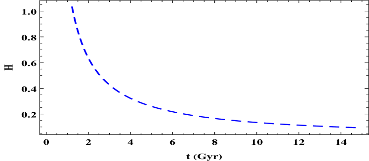
(a) $n=1.25$, $b=0.20$, $t_{0}=0.57$

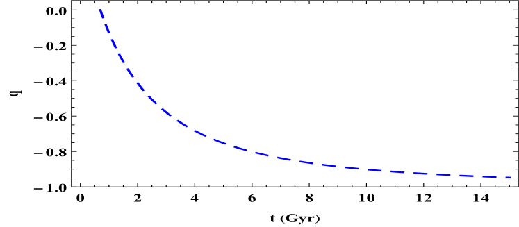
(b) $n=1.25,b=0.20,t_{0}=0.57$

Figure 1: The plot of Hubble’s parameter $(H)$ and Deceleration parameter $(q)$ Vs cosmic time $(t)$

5 Geometrical and physical significance of the model

From equations (23), (27), (30) and (32) we have obtained the energy density as

$$\rho=\frac{-1}{16\pi}\biggl{\{}-18\alpha E-18^{m}(2m-1)\beta E^{m}\biggr{\}}$$ (37)

where,

$$E=\biggl{[}\frac{-(1+2k)(bt+nt_{0})^{2}}{(k+2)^{2}t^{2}t_{0}^{2}}\biggr{]}$$

The coefficient of bulk viscosity parameter $(\xi)$ is obtained from equations (25) and(26) as

$$\xi=\frac{\rho\gamma}{3H}$$ (38)

The bulk viscosity coefficient $\xi$ consistently decreases with time, maintaining a positive value throughout cosmic evolution as per figure (4(a)) (left panel). They are ultimately leading to the emergence of inflationary models. Additionally, the models do not exhibit an initial singularity, supporting Murphy’s [97] conclusion that the introduction of bulk viscosity successfully avoids such singularities. This observed behaviour aligns well with the anticipated physical characteristics of $\xi$, and these reports are in good agreement with [98, 99].

The bulk viscous pressure $(\bar{p})$ is obtained from equations (27), (29) and (32) as

$$\begin{split}\bar{p}=&\frac{1}{16\pi(2+k)^{2}t^{2}t_{0}^{2}}\Bigg{\{}18\alpha(1+2k)(bt+nt_{0})^{2}+mn\beta t_{0}(2+k)(1+k)(1-m)^{2}2^{(1+m)}3^{(-1+2m)}\\ &\ E^{(-1+m)}-18^{m}t^{2}\beta t_{0}^{2}(2+k)^{2}E^{m}+6(1+k)\biggl{(}3b^{2}kt^{2}+6bkntt_{0}+n(-2+k(-1+3n))t_{0}^{2}\biggr{)}\\ &\ \biggl{(}\alpha+18^{(-1+m)}m\beta E^{(-1+m)}\biggr{)}\Biggr{\}}\end{split}$$ (39)

The string tension density ($\lambda$) is obtained from equations (27), (28), (32) and (39) as

$$\begin{split}\lambda=&\frac{(-1+k)}{8\pi(2+k)^{2}t^{2}t_{0}^{2}}\Biggl{\{}mn\beta t_{0}^{2}(2+k)(1-m)2^{m}3^{(-1+2m)}E^{(-1+m)}+3\biggl{(}3b^{2}(4+k)t^{2}+6b(4+k)ntt_{0}\\ &\ +n(-2-k+3(4+k)n)t_{0}^{2}\biggr{)}\biggl{(}\alpha+18^{(-1+m)}m\beta E^{(-1+m)}\biggr{)}\Biggr{\}}\end{split}$$ (40)

We have noted that the string tension density $\lambda$ exhibits a positive correlation with time, always maintaining a negative value until it eventually converges to zero at a subsequent point in time. Letelier [68] highlighted the potential occurrence of both positive and negative values for $\lambda$. In the case where $\lambda<0$, the string phase of the universe ceases to exist, resulting in the presence of an anisotropic fluid comprised of particles. This characteristic behaviour of $\lambda$ is also depicted in figure (6(a)) (left panel). Our findings show comparable outcomes with [100, 101].

The particle energy density $(\rho_{p})$ is calculated from equations (39) and (40) as

$$\begin{split}\rho_{p}=&\frac{1}{16\pi(2+k)^{2}t^{2}t_{0}^{2}}\Biggl{\{}18\alpha(1+2k)(bt+nt_{0})^{2}+18^{m}\beta t^{2}t_{0}^{2}(2+k)^{2}(1-2m)E^{m}+2(1-k)\Biggl{[}mn\beta\\ &\ t_{0}^{2}(2+k)(1-m)2^{m}3^{(-1+2m)}E^{(-1+m)}+3\biggl{(}3b^{2}(4+k)t^{2}+6b(4+k)ntt_{0}+n(-2-k+3(4\\ &\ +k)n)t_{0}^{2}\biggr{)}\biggl{(}\alpha+18^{(-1+m)}m\beta E^{(-1+m)}\biggr{)}\Biggr{]}\Biggr{\}}\end{split}$$ (41)

The proper energy density $\rho$ and particle density $\rho_{p}$ exhibit a swift decline from positive values to the same constant as shown in figures (2(a)) (left panel) and (2(b)) (right panel). The substantial initial values of $\rho$ and $\rho_{p}$ figure (2) signify the domination of densities during the early stages, diminishing significantly as time progresses. Importantly, $\rho$ and $\rho_{p}$ maintain positive values throughout the entire evolution of the universe. This trend underscores the expansive nature of the universe. According to [41] $\rho\rightarrow 0$, $\rho_{p}\rightarrow 0$ for $t\rightarrow\infty$ thus the universe approaches a flat universe at late time. As a result, our model is in good agreement with the recent observation, these respondents have strong agreement with [102, 103, 104].

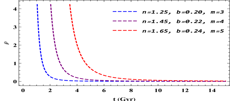
(a) $\alpha=0.01,\beta=0.056,k=1.2,t_{0}=0.57$

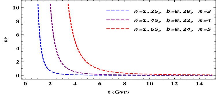
(b) $\alpha=0.01,\beta=0.056,k=1.2,t_{0}=0.57$

Figure 2: Plot of energy density $(\rho)$ and particle energy density $(\rho_{p})$ conditions Vs cosmic time $(t)$

From equations (25), (35), (38) and (39) The proper pressure $(p)$ is calculated as

$$\begin{split}p=&\frac{1}{16\pi(2+k)^{2}t^{2}t_{0}^{2}}\Bigg{\{}18\alpha(1+2k)(bt+nt_{0})^{2}+mnt_{0}^{2}(2+k)(1+k)(1-m)2^{(1+m)}3^{(-1+2m)}\\ &\ E^{(-1+m)}\beta-18^{m}\beta(2+k)^{2}t^{2}t_{0}^{2}E^{m}+6(1+k)\biggl{(}3b^{2}kt^{2}+6bkntt_{0}+n(-2+k(-1+3n))t_{0}^{2}\biggr{)}\\ &\ \biggl{(}\alpha+18^{(-1+m)}m\beta E^{(-1+m)}\biggr{)}+\beta\Biggl{(}18\alpha(1+2k)(bt+nt_{0})^{2}\alpha+18^{m}\beta(2+k)^{2}(1-2m)t^{2}t_{0}^{2}\\ &\ E^{m}\Biggr{)}\Biggr{\}}\end{split}$$ (42)

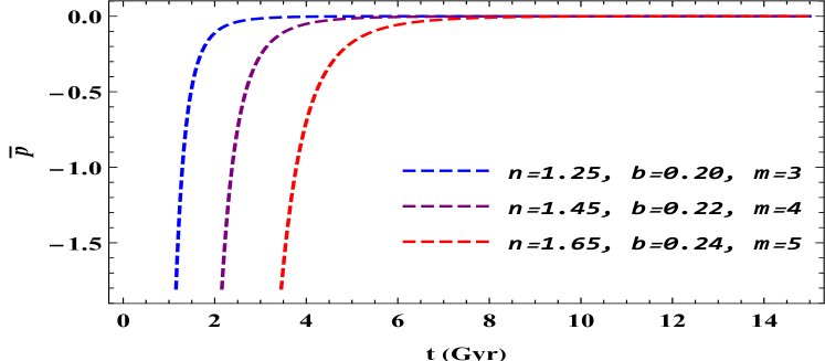
(a) $\alpha=0.01,\beta=0.056,k=1.2,t_{0}=0.57$

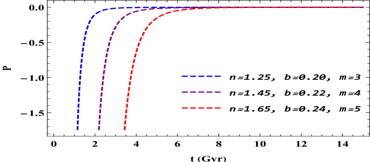
(b) $\alpha=0.01,\beta=0.056,k=1.2,t_{0}=0.57$

Figure 3: Plot of pressure $(\bar{p})$ and bulk viscous pressure particle energy density $(p)$ conditions Vs cosmic time $(t)$

The examination of figures (3(a)) (left panel) and (3(b)) (right panel) reveals a noteworthy trend in the behaviour of bulk viscous ${\bar{p}}$ pressure and pressure $p$ across cosmic evolution. Both parameters ${\bar{p}}$ and $p$ figure (3) consistently exhibit a negative trajectory throughout this evolution, beginning with substantial negative values and at the present epoch $\bar{p}\rightarrow 0$ and $p\rightarrow 0$ this characteristic behaviour implies a phase of accelerated expansion in the universe. The persistent negativity in pressure and bulk viscous pressure signifies a sustained repulsive effect, contributing to the observed cosmic acceleration, these arguments hold similar results with [102, 103, 104, 100, 101].

The equation of state parameter (EoS) is given by

$$\omega=\frac{p}{\rho}$$ (43)

Currently one of the largest endeavours in observational cosmology is the measurement of the EoS parameter for dark energy (DE). The traditional description of the DE model is provided by the EoS parameter $\omega=\frac{p}{\rho}$, which not necessarily be constant. Figure (4(b)) (right panel) portrays the behaviour of the EoS parameter along with cosmic time using hybrid expansion law for some fixed values of $n$, $b$ and $m$. It is clear that at the present epoch $-1\leq\omega<0$ and $\omega\leq-1$ in the recent past thus the model shows a phase transition from the phantom era to the quintessence era and this holds a good agreement with [104, 105, 106].

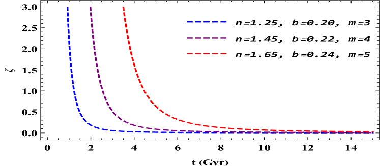
(a) $\alpha=0.01,\beta=0.056,k=1.2,t_{0}=0.57$

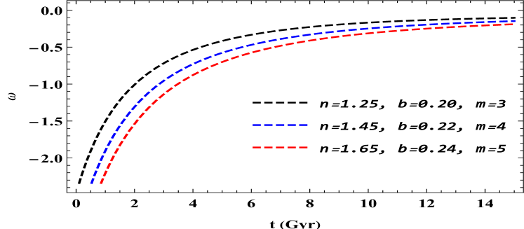
(b) $\alpha=0.01,\beta=0.056,k=1.2,t_{0}=0.57$

Figure 4: Plot of coefficient of bulk viscosity $(\xi)$ and EoS parameter $(\omega)$ Vs cosmic time $(t)$

The anisotropic parameter $(A_{m})$, expansion scalar $(\theta)$, shear scalar $(\sigma^{2})$ are given as

$$A_{m}=\frac{2(k-1)^{2}}{(k+2)^{2}}$$ (44)

$$\theta=\frac{3(bt+nt_{0})}{tt_{0}}$$ (45)

$$\sigma^{2}=\frac{3(k-1)(bt+nt_{0})^{2}}{(k+2)^{2}t^{2}t_{0}^{2}}$$ (46)

From equations (45) and (46), it is seen that $\theta\rightarrow 0$ and $\sigma^{2}\rightarrow 0$ as $t\rightarrow\infty$ and they both get diverges as $t\rightarrow 0$ as shown in figure (5(a)) (left panel) and (5(b)) (right panel). It is observed from equation (44) that for $k\neq 1$ we got $A_{m}\neq 0$ this infers that our constructed model of the universe remains anisotropic throughout cosmic evolution.

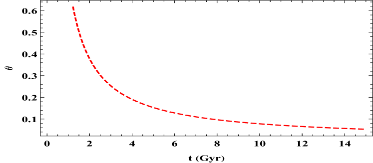
(a) $\alpha=0.01,\beta=0.056,k=1.2,t_{0}=0.57$

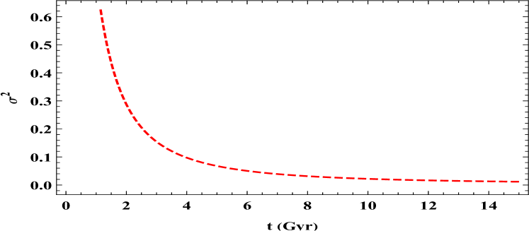
(b) $\alpha=0.01,\beta=0.056,k=1.2,t_{0}=0.57$

Figure 5: Plot of expansion scalar $(\theta)$ and shear scalar $(\sigma^{2})$ conditions Vs cosmic time $(t)$

5.1 Energy conditions

Numerous methods are employed to figure out the universe’s history and are used in many approaches to understanding the evolution of the universe. Energy conditions play a crucial role in confirming hypotheses about the singularity of space-time and black holes [107], including those put forth by Roger Penrose and Stephen Hawking [108]. Verifying the universe’s expansion is the primary goal of these energy conditions in this context. Energy conditions can take many different forms, including dominant energy condition (DEC), weak energy condition (WEC), null energy condition (NEC), and strong energy condition these conditions are given as [109].

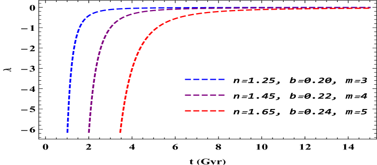
(a) $\alpha=0.01,\beta=0.056,k=1.2,t_{0}=0.57$

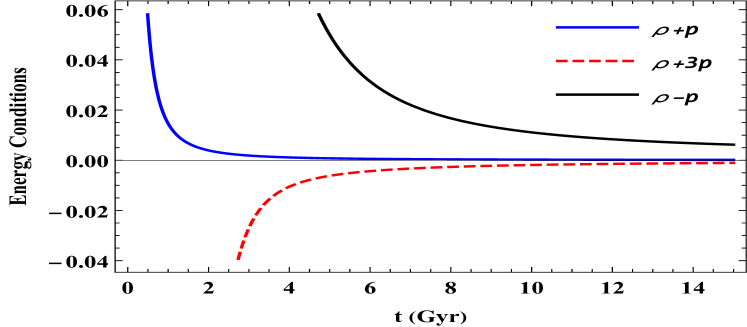
(b) $\alpha=0.01,\beta=0.056,k=1.2,t_{0}=0.57$

Figure 6: Plot of string energy density $(\lambda)$ and energy conditions conditions Vs cosmic time $(t)$

1). $\rho\geq 0,$  $\rho\pm\bar{p}\geq 0$, (DEC)   2). $\rho\geq 0$,  $\rho-\bar{p}\geq 0$ (WEC)   3). $\rho+\bar{p}\geq 0$,  $\rho+3\bar{p}\geq 0$ (SEC)

From figure (6(b)) (right panel) the weak energy condition (WEC) and dominant energy condition (DEC) are satisfied for the constructed model. However, the strong energy condition (SEC) is violated. There is a reverse gravitational impact when the (SEC) is violated. The cosmos jerks as a result, and the current acceleration phase gives way to the previous deceleration phase [110]. As a result, the model proposed in this research appears to be a good fit for explaining the universe’s late temporal acceleration.

6 Conclusion

Here we have discussed spatially homogeneous and anisotropic Kantowski-Sachs space-time in the presence of bulk viscous fluid with one-dimensional cosmic strings in $f(T)$ gravity by modifying general relativity to explain the challenging problem of late time acceleration of the universe. To obtain a definite solution to the highly non-linear field equations (14)$-$(16) of this theory, we have taken the help of the special law of variation (23)$-$(25). It is interesting to observe that,

• The Hubble parameter $(H)$ figure (1(a)) (left panel) diminishes and ultimately approaches a small value with the passage of cosmic time. The deceleration parameter $(q)$ figure (1(b)) (right panel) shows phase transition as its value changes from positive to negative. It shows early deceleration to late time acceleration, hence for the late time our model shows $H>0$, $q<0$ implies the model shows the expanding and accelerating nature of the universe.

• Figure (2) represent the behaviour of proper energy density $(\rho)$ and particle energy density $(\rho_{p})$. It is observed that both are positive decreasing functions of time which shows the expansion nature of the universe.

• Eventually, we arrive at an inflationary model since the bulk viscosity $(\xi)$ diminishes with time (4(a)).

• The negative pressure $(p)$ and $(\bar{p})$ figure (3) corresponds to cosmic acceleration according to standard cosmology. Therefore, constructed models of the universe show an accelerated expansion phase at present as well as in future.

• The string energy density $(\lambda)$ is negative throughout cosmic evolution figure (6(a)) (left panel) and at the late time it approaches zero this means at the present epoch we get string free model. When $\lambda<0$, the string phase of the universe disappears i.e. we have an anisotropic fluid of particles.

• The EoS parameter $(\omega)$ figure (4(b)) (right panel) resembles the dark energy model and behaves like the quintessence model $-1\leq\omega<0$ at present.

• The Energy Conditions figure (6(b)) (right panel) namely WEC, DEC and SEC, we confirmed that WEC and DEC are valid but violate SEC. The violation of SEC gives an anti-gravitational effect for which the universe gets jerked and thus our Universe exhibits a transition from early decelerating to the present accelerating Universe.

References

- Riess et al. [(1998] A. G. Riess, A. V. Filippenko, P. Challis, A. Clocchiatti, A. Diercks, P. M. Garnavich, R. L. Gilliland, C. J. Hogan, S. Jha, R. P. Kirshner et al., The astronomical journal, (1998), 116, 1009.
- Perlmutter et al. [(1999] S. Perlmutter, G. Aldering, G. Goldhaber, R. Knop, P. Nugent, P. G. Castro, S. Deustua, S. Fabbro, A. Goobar, D. E. Groom et al., The Astrophysical Journal, (1999), 517, 565.
- Eisenstein et al. [(2005] D. J. Eisenstein, I. Zehavi, D. W. Hogg, R. Scoccimarro, M. R. Blanton, R. C. Nichol, R. Scranton, H.-J. Seo, M. Tegmark, Z. Zheng et al., The Astrophysical Journal, (2005), 633, 560.
- Percival et al. [(2010] W. J. Percival, B. A. Reid, D. J. Eisenstein, N. A. Bahcall, T. Budavari, J. A. Frieman, M. Fukugita, J. E. Gunn, Ž. Ivezić, G. R. Knapp et al., Monthly Notices of the Royal Astronomical Society, (2010), 401, 2148–2168.
- Koivisto and Mota [(2006] T. Koivisto and D. F. Mota, Physical Review D, (2006), 73, 083502.
- Daniel et al. [(2008] S. F. Daniel, R. R. Caldwell, A. Cooray and A. Melchiorri, Physical Review D, (2008), 77, 103513.
- Fedeli et al. [(2009] C. Fedeli, L. Moscardini and M. Bartelmann, Astronomy & Astrophysics, (2009), 500, 667–679.
- Caldwell and Doran [(2004] R. R. Caldwell and M. Doran, Physical Review D, (2004), 69, 103517.
- Huang et al. [(2006] Z.-Y. Huang, B. Wang, E. Abdalla and R.-K. Su, Journal of Cosmology and Astroparticle Physics, (2006), 2006, 013.
- Gadbail et al. [(2021] G. N. Gadbail, S. Arora and P. Sahoo, The European Physical Journal C, (2021), 81, 1088.
- Capozziello et al. [(2011] S. Capozziello, V. Cardone, H. Farajollahi and A. Ravanpak, Physical Review D, (2011), 84, 043527.
- Tsujikawa [(2011] S. Tsujikawa, in Dark Matter and Dark Energy: A Challenge for Modern Cosmology, Springer, (2011), pp. 331–402.
- Yang and Zhang [(2010] R.-J. Yang and S. N. Zhang, Monthly Notices of the Royal Astronomical Society, (2010), 407, 1835–1841.
- Feng et al. [(2005] B. Feng, X. Wang and X. Zhang, Physics Letters B, (2005), 607, 35–41.
- Copeland et al. [(2006] E. J. Copeland, M. Sami and S. Tsujikawa, International Journal of Modern Physics D, (2006), 15, 1753–1935.
- Carroll [(1998] S. M. Carroll, Physical Review Letters, (1998), 81, 3067.
- Fujii [(1982] Y. Fujii, Physical Review D, (1982), 26, 2580.
- Chiba et al. [(2000] T. Chiba, T. Okabe and M. Yamaguchi, Physical Review D, (2000), 62, 023511.
- Armendariz-Picon et al. [(2000] C. Armendariz-Picon, V. Mukhanov and P. J. Steinhardt, Physical Review Letters, (2000), 85, 4438.
- Bento et al. [(2002] M. Bento, O. Bertolami and A. A. Sen, Physical Review D, (2002), 66, 043507.
- Kamenshchik et al. [(2001] A. Kamenshchik, U. Moschella and V. Pasquier, Physics Letters B, (2001), 511, 265–268.
- Solanki et al. [(2021] R. Solanki, S. Pacif, A. Parida and P. Sahoo, Physics of the Dark Universe, (2021), 32, 100820.
- Buchdahl [(1970] H. A. Buchdahl, Monthly Notices of the Royal Astronomical Society, (1970), 150, 1–8.
- Harko et al. [(2011] T. Harko, F. S. Lobo, S. Nojiri and S. D. Odintsov, Physical Review D, (2011), 84, 024020.
- Shabani and Farhoudi [(2013] H. Shabani and M. Farhoudi, Phys. Rev. D, (2013), 88, 044048.
- Sahoo et al. [(2018] P. Sahoo, P. Moraes and P. Sahoo, The European Physical Journal C, (2018), 78, 1–7.
- De Felice and Tsujikawa [(2009] A. De Felice and S. Tsujikawa, Physics Letters B, (2009), 675, 1–8.
- Goheer et al. [(2009] N. Goheer, R. Goswami, P. K. Dunsby and K. Ananda, Physical Review D, (2009), 79, 121301.
- Bamba et al. [(2017] K. Bamba, M. Ilyas, M. Bhatti and Z. Yousaf, General Relativity and Gravitation, (2017), 49, 1–17.
- Elizalde et al. [(2010] E. Elizalde, R. Myrzakulov, V. V. Obukhov and D. Sáez-Gómez, Classical and Quantum Gravity, (2010), 27, 095007.
- Bamba et al. [(2010] K. Bamba, S. D. Odintsov, L. Sebastiani and S. Zerbini, The European Physical Journal C, (2010), 67, 295–310.
- Ferraro and Fiorini [(2007] R. Ferraro and F. Fiorini, Physical Review D, (2007), 75, 084031.
- Linder [(2010] E. V. Linder, Physical Review D, (2010), 81, 127301.
- Bamba et al. [2011] K. Bamba, C.-Q. Geng, C.-C. Lee and L.-W. Luo, Journal of Cosmology and Astroparticle Physics, 2011, (2011), 021.
- Bahamonde et al. [(2017] S. Bahamonde, S. Capozziello, M. Faizal and R. C. Nunes, The European Physical Journal C, (2017), 77, 1–8.
- Arora et al. [(2021] S. Arora, J. Santos and P. Sahoo, Physics of the Dark Universe, (2021), 31, 100790.
- Xu et al. [(2019] Y. Xu, G. Li, T. Harko and S.-D. Liang, The European Physical Journal C, (2019), 79, 1–19.
- Solanke et al. [(2023] Y. Solanke, A. Kale, D. Pawar and V. Dagwal, Canadian Journal of Physics, (2023), 102, 85–95.
- Nojiri et al. [(2008] S. Nojiri, S. D. Odintsov and P. V. Tretyakov, Progress of Theoretical Physics Supplement, (2008), 172, 81–89.
- Unzicker and Case [(2005] A. Unzicker and T. Case, arXiv preprint physics/0503046, (2005).
- Bhoyar et al. [(2017] S. Bhoyar, V. Chirde and S. Shekh, Astrophysics, (2017), 60, 259–272.
- Dagwal and Pawar [(2020] V. Dagwal and D. Pawar, Modern Physics Letters A, (2020), 35, 1950357.
- Myrzakulov [(2011] R. Myrzakulov, The European Physical Journal C, (2011), 71, 1752.
- Li et al. [(2011] B. Li, T. P. Sotiriou and J. D. Barrow, Physical Review D, (2011), 83, 104017.
- Rodrigues et al. [(2012] M. Rodrigues, M. Houndjo, D. Saez-Gomez and F. Rahaman, Physical Review D, (2012), 86, 104059.
- Brevik et al. [(2012] I. Brevik, R. Myrzakulov, S. Nojiri and S. Odintsov, Physical Review D, (2012), 86, 063007.
- Barrow and Matzner [(1977] J. D. Barrow and R. A. Matzner, Monthly Notices of the Royal Astronomical Society, (1977), 181, 719–727.
- Colistete Jr et al. [(2007] R. Colistete Jr, J. Fabris, J. Tossa and W. Zimdahl, Physical Review D, (2007), 76, 103516.
- Capozziello et al. [(2006] S. Capozziello, V. F. Cardone, E. Elizalde, S. Nojiri and S. D. Odintsov, Physical Review D, (2006), 73, 043512.
- Zimdahl et al. [(2001] W. Zimdahl, D. J. Schwarz, A. B. Balakin and D. Pavon, Physical Review D, (2001), 64, 063501.
- Velten and Schwarz [(2012] H. Velten and D. J. Schwarz, Physical Review D, (2012), 86, 083501.
- Bamba and Odintsov [(2016] K. Bamba and S. D. Odintsov, The European Physical Journal C, (2016), 76, 1–12.
- Arora et al. [(2022] S. Arora, S. Pacif, A. Parida and P. Sahoo, Journal of High Energy Astrophysics, (2022), 33, 1–9.
- Ren and Meng [(2006] J. Ren and X.-H. Meng, Physics Letters B, (2006), 636, 5–12.
- Brevik and Normann [(2020] I. Brevik and B. D. Normann, Symmetry, (2020), 12, 1085.
- Brevik and Grøn [(2013] I. Brevik and Ø. Grøn, Astrophysics and Space Science, (2013), 347, 399–404.
- Padmanabhan and Chitre [(1987] T. Padmanabhan and S. Chitre, Physics Letters A, (1987), 120, 433–436.
- Capozziello et al. [(2006] S. Capozziello, S. Nojiri and S. Odintsov, Physics Letters B, (2006), 632, 597–604.
- Wang et al. [(2017] D. Wang, Y.-J. Yan and X.-H. Meng, The European Physical Journal C, (2017), 77, 660.
- Mak and Harko [(2003] M. Mak and T. Harko, International Journal of Modern Physics D, (2003), 12, 925–939.
- Bali and Pradhan [(2007] R. Bali and A. Pradhan, Chinese Physics Letters, (2007), 24, 585.
- Kibble [(1976] T. W. Kibble, Journal of Physics A: Mathematical and General, (1976), 9, 1387.
- Zel’dovich et al. [(1974] Y. B. Zel’dovich, I. Y. Kobzarev and L. B. Okun, Zh. Eksp. Teor. Fiz., (1974), 40, 3–11.
- Kibble [(1980] T. W. Kibble, Physics Reports, (1980), 67, 183–199.
- Everett [(1981] A. E. Everett, Physical Review D, (1981), 24, 858.
- Vilenkin [(1981] A. Vilenkin, Physical Review D, (1981), 24, 2082.
- Letelier [(1979] P. S. Letelier, Physical Review D, (1979), 20, 1294.
- [68] P. S. Letelier, Physical review D, 28, 2414.
- Stachel [(1980] J. Stachel, Physical Review D, (1980), 21, 2171.
- Banerjee et al. [(1990] A. Banerjee, A. K. Sanyal and S. Chakraborty, Pramana, (1990), 34, 1–11.
- Chakraborty [(1991] S. Chakraborty, Indian Journal of Pure and Applied Physics, (1991), 29, 31–33.
- Ram and Singh [(1995] S. Ram and J. Singh, General Relativity and Gravitation, (1995), 27, 1207–1213.
- Yilmaz [(2006] İ. Yilmaz, General Relativity and Gravitation, (2006), 38, 1397–1406.
- Ryan and Shepley [(2015] M. P. Ryan and L. C. Shepley, Homogeneous relativistic cosmologies, Princeton University Press, (2015), vol. 65.
- Misner [(1968] C. W. Misner, The Astrophysical Journal, (1968), 151, 431.
- Weber [(1984] E. Weber, Journal of mathematical physics, (1984), 25, 3279–3285.
- Weber [(1985] E. Weber, Journal of mathematical physics, (1985), 26, 1308–1310.
- Grøn and Eriksen [(1987] Ø. Grøn and E. Eriksen, Physics Letters A, (1987), 121, 217–220.
- Collins [(1977] C. Collins, Journal of Mathematical Physics, (1977), 18, 2116–2124.
- Dhurandhar et al. [(1980] S. Dhurandhar, C. Vishveshwara and J. M. Cohen, Physical Review D, (1980), 21, 2794.
- Banerjee and Ghosh [(1999] A. Banerjee and T. Ghosh, Classical and Quantum Gravity, (1999), 16, 3981.
- Garcia-Salcedo and Bretón [(2005] R. Garcia-Salcedo and N. Bretón, Classical and Quantum Gravity, (2005), 22, 4783.
- Bruni et al. [(1994] M. Bruni, S. Matarrese and O. Pantano, arXiv preprint astro-ph/9406068, (1994).
- Szekeres [(1975] P. Szekeres, Communications in Mathematical Physics, (1975), 41, 55–64.
- Bonnor and Tomimura [(1976] W. B. Bonnor and N. Tomimura, Monthly Notices of the Royal Astronomical Society, (1976), 175, 85–93.
- Akarsu et al. [(2014] Ö. Akarsu, S. Kumar, R. Myrzakulov, M. Sami and L. Xu, Journal of Cosmology and Astroparticle Physics, (2014), 2014, 022.
- Shekh [(2015] S. B. V. C. S. Shekh, International Journal, (2015), 3, 492–500.
- Collins et al. [(1980] C. Collins, E. Glass and D. Wilkinson, General Relativity and Gravitation, (1980), 12, 805–823.
- Prasanthi and Aditya [(2020] U. D. Prasanthi and Y. Aditya, Results in Physics, (2020), 17, 103101.
- Reddy et al. [2013] D. Reddy, P. Rao, T. Vidyasagar, R. Bhuvana Vijaya et al., Advances in High Energy Physics, 2013, (2013), .
- Naidu et al. [(2013] R. Naidu, D. Reddy, T. Ramprasad and K. Ramana, Astrophysics and Space Science, (2013), 348, 247–252.
- Bhoyar et al. [(2019] S. Bhoyar, V. Chirde and S. Shekh, Journal of Scientific Research, (2019), 11, .
- Vidyasagar et al. [(2014] T. Vidyasagar, R. Naidu, R. Bhuvana Vijaya and D. Reddy, The European Physical Journal Plus, (2014), 129, 1–7.
- Mishra and Dua [(2019] R. Mishra and H. Dua, Astrophysics and Space Science, (2019), 364, 195.
- Yadav [(2012] A. K. Yadav, Research in Astronomy and Astrophysics, (2012), 12, 1467.
- Bharali and Das [(2023] J. Bharali and K. Das, Bulgarian Journal of Physics, (2023), 50, .
- Murphy [(1973] G. L. Murphy, Physical Review D, (1973), 8, 4231.
- Reddy et al. [(2013] D. Reddy, P. Rao, T. Vidyasagar, R. Bhuvana Vijaya et al., Advances in High Energy Physics, (2013), 2013, .
- Pawar and Dabre [(2022] K. Pawar and A. Dabre, Int. J. Sci. Res. in Physics and Applied Sciences Vol, (2022), 10, .
- Amirhashchi et al. [(2011] H. Amirhashchi, H. Zainuddin and A. Pradhan, International Journal of Theoretical Physics, (2011), 50, 2531–2545.
- Amirhashchi [(2013] H. Amirhashchi, Pramana, (2013), 80, 723–738.
- Reddy et al. [(2013] D. Reddy, R. Naidu, K. Dasu Naidu and T. Ram Prasad, Astrophysics and Space Science, (2013), 346, 261–265.
- Moreira and Almeida [(2023] A. Moreira and C. Almeida, General Relativity and Gravitation, (2023), 55, 89.
- Sahoo et al. [(2016] P. Sahoo, B. Mishra, P. Sahoo and S. Pacif, The European Physical Journal Plus, (2016), 131, 1–12.
- Santhi et al. [(2022] M. V. Santhi, A. S. Rao, T. Chinnappalanaidu and S. S. Madhu, Mathematical Statistician and Engineering Applications, (2022), 71, 1056–1072.
- Rodrigues et al. [(2015] M. Rodrigues, A. Kpadonou, F. Rahaman, P. Oliveira and M. Houndjo, Astrophysics and Space Science, (2015), 357, 1–7.
- Wald [(2010] R. M. Wald, General relativity, University of Chicago press, (2010).
- Ellis [(2014] G. F. Ellis, The European Physical Journal H, (2014), 39, 403–411.
- Koussour and Bennai [(2022] M. Koussour and M. Bennai, International Journal of Geometric Methods in Modern Physics, (2022), 19, 2250038.
- Caldwell et al. [(2006] R. R. Caldwell, W. Komp, L. Parker and D. A. Vanzella, Physical Review D, (2006), 73, 023513.