COMMIT: Certifying Robustness of Multi-Sensor Fusion Systems against Semantic Attacks

Abstract

Multi-sensor fusion systems (MSFs) play a vital role as the perception module in modern autonomous vehicles (AVs). Therefore, ensuring their robustness against common and realistic adversarial semantic transformations, such as rotation and shifting in the physical world, is crucial for the safety of AVs. While empirical evidence suggests that MSFs exhibit improved robustness compared to single-modal models, they are still vulnerable to adversarial semantic transformations. Despite the proposal of empirical defenses, several works show that these defenses can be attacked again by new adaptive attacks. So far, there is no certified defense proposed for MSFs. In this work, we propose the first robustness certification framework COMMIT to certify robustness of multi-sensor fusion systems against semantic attacks. In particular, we propose a practical anisotropic noise mechanism that leverages randomized smoothing with multi-modal data and performs a grid-based splitting method to characterize complex semantic transformations. We also propose efficient algorithms to compute the certification in terms of object detection accuracy and IoU for large-scale MSF models. Empirically, we evaluate the efficacy of COMMIT in different settings and provide a comprehensive benchmark of certified robustness for different MSF models using the CARLA simulation platform. We show that the certification for MSF models is at most 48.39% higher than that of single-modal models, which validates the advantages of MSF models. We believe our certification framework and benchmark will contribute an important step towards certifiably robust AVs in practice.

1 Introduction

Autonomous driving (AD) has achieved significant advances in recent years [37, 25, 1, 54, 56, 31, 36, 5], and deep neural networks (DNNs) have been largely deployed as the perception module for AD to process inputs from multiple sources (e.g., camera and LiDAR) to detect objects such as road signs, vehicles, and pedestrians. To make full use of multi-modal inputs, modern AD systems usually adopt the multi-sensor fusion systems (MSFs) as the perception module [34, 6].

Along with the wide deployment of AD systems, the safety of AD systems in the physical world has raised serious concerns [18, 2]. A rich body of research has shown that both adversarial perturbations and natural semantic transformations can mislead the DNN-based perception modules in AD systems with a high success rate [35, 21, 48, 16, 19, 12], so that the AD system may ignore the pedestrians, the traffic signs, or other vehicles with high confidence when the object is slightly rotated or shifted, which can lead to severe consequences such as fatal traffic accidents [33]. Moreover, even though the multi-sensor fusion systems may be intuitively more robust, assuming that the input transformations/perturbations are not adversarial to multiple input modalities at the same time, existing work [2, 17] has falsified such intuition by proposing feasible and highly efficient attacks against multi-sensor fusion systems [2]. In other words, serious robustness issues still exist in existing MSFs, resulting in practical safety vulnerabilities in AD.

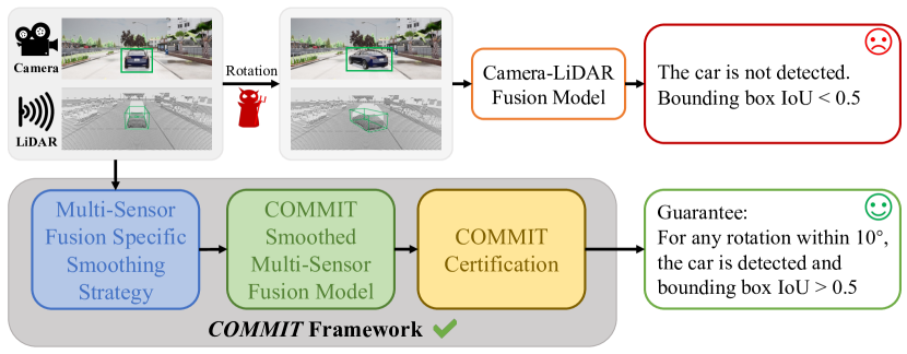
Figure 1: Overview of COMMIT, the first framework that provides certified robustness for multi-sensor fusion systems against semantic transformations.

To mitigate such safety threats, several empirical defenses have been proposed for both single-modal models [32] and multi-sensor fusion systems [55]. However, certified defenses exist only for single-modal models [47, 9, 26, 8]. Recent works have shown that the empirical defenses for MSFs can be adaptively attacked again by stealthy perturbations or transformations [55, 22]. In this paper, we aim to provide the first robustness certification and enhancement framework for multi-sensor fusion systems in AD against various semantic transformations in the physical world.

Our framework leverages the randomized smoothing technique [9], while randomized smoothing cannot directly provide a robustness guarantee against semantic transformations (e.g., object rotation and shifting) for multi-sensor fusion systems due to three main reasons: (1) Heterogeneous input dimensions: In randomized smoothing, the isotropic noise is added to all input dimensions, which is sub-optimal for multi-sensor fusion systems since different input modalities need different noises. (2) Intractable perturbation spaces: Semantic transformations incur large $\ell_{p}$ that cannot be handled by classical randomized smoothing [51], and the transformation function does not have a closed-form expression that is required for semantic-smoothing-based certification [26]. (3) Unsupported certification criterion: Existing randomized smoothing techniques are designed for certifying output consistency for classification [9] and regression [24] tasks. However, multi-sensor fusion systems output 3D bounding boxes for detected objects and use IoU as the evaluation criterion, while randomized smoothing cannot provide worst-case certification for IoU.

To solve these challenges, our framework COMMIT provides the following techniques: (1) We derive an anisotropic noise mechanism that is practical (agnostic to the transformations to be certified) and efficient for randomized smoothing over multi-modal data. (2) Under a mild assumption, we propose a grid-based splitting method to integrate small $\ell_{p}$ certifications and form a holistic certification against complex semantic transformations. (3) We derive the first rigorous lower bounds of detection confidence and lower bounds of IoU for MSF models.

We leverage our framework to certify the state-of-the-art large-scale camera and LiDAR fusion 3D object detection models (CLOCs [34] and FocalsConv [6]) and compare them with a camera-based 3D object detector (MonoCon [30]) as well as one LiDAR-based 3D object detector (SECOND [50]) in CARLA simulator. We consider transformations such as rotation and shifting, which correspond to the turning around and sudden brake cases in the real world. In particular, we are able to achieve 100.00% certified detection accuracy and 53.23% certified IoU under rotation transformations. Compared to single-modal models, the certification improvements are 25.19% and 53.23%, respectively. We demonstrate that the certified robustness depends on both the input and the fusion pipeline structure.

Technical Contributions.

In this paper, we provide the first certification framework for multi-sensor fusion systems against adversarial semantic transformations. We make contributions on both theoretical and empirical fronts.

• We propose the first generic framework for certifying the robustness of multi-sensor fusion systems against practical semantic transformations in the physical world.

• We propose a practical anisotropic noise mechanism to leverage randomized smoothing given multi-modal data, a grid-based splitting method to characterize complex semantic transformations, and efficient algorithms to compute the certification for object detection and IoU lower bounds for large-scale MSF models.

• We construct extensive experiments and provide a benchmark of certified robustness for multi-sensor fusion systems based on COMMIT. We certify several state-of-the-art camera-LiDAR fusion models and compare them with single-modal models. We show that the multi-sensor fusion systems provide nontrivial gains on certified robustness, e.g., achieving 53.23% improvement against the rotation transformation. In addition, we present several interesting observations which would further inspire the development of robust sensor fusion algorithms. The benchmark will be open source upon acceptance and will be continuously expanding to evaluate more AD systems.

2 Related Work

Multi-sensor fusion systems. Multi-sensor fusion DNN systems leverage data of multiple modalities to predict 3D bounding boxes for object detection. In this work, we consider multi-sensor fusion systems that take both image (from a camera) and point clouds (from a LiDAR sensor) for object detection [34, 6], which is one of the most common forms of AD perception module [42]. These fusion systems typically integrate outputs from sub-models for each modality via learning-based methods or aggregation rules. Note that our framework is architecture-agnostic — applicable for any fusion system regardless of their internal architectures.

Adversarial attacks for DNNs. The robustness vulnerabilities of DNNs are manifested by adversarial attacks. A rich body of research shows that DNNs can be attacked by pixel-wise perturbations bounded by small $\ell_{p}$ norm with even 100% success rate [46, 15, 4]. Besides $\ell_{p}$-bounded perturbations, subsequent research shows that spatial transformations [48], occlusions [44], and semantic transformations that naturally exist [35, 19, 14] can also mislead DNNs to make severe incorrect predictions. In particular, several physically realizable and effective adversarial attacks have been proposed against multi-sensor fusion systems [13, 2], posing serious safety threats to modern AD.

Certified robustness for DNNs. To mitigate the robustness vulnerabilities, several defenses are proposed, which can be roughly categorized into empirical and certified defenses. The empirical defenses [32, 40, 41] train DNNs with heuristic approaches, e.g., adversarial training, to defend against adversarial attacks. However, they cannot provide rigorous robustness guarantees against possible future attacks. In contrast, certified defenses can prove that the trained DNNs are certifiably robust against any possible attacks under some perturbation constraints [27]. Certified defenses are mainly based on verification methods like linear relaxations with branch-and-bound [47, 53], Lipschitz DNN architectures [52, 43, 49], and randomized smoothing [9, 51, 7, 28, 45, 3].

For multi-sensor fusion systems, although some empirical defenses have been proposed [29, 55], there is no certified defense that provides robustness guarantees to our best knowledge. Thus, here we aim to provide the first robustness certification and enhancement framework for MSF models.

3 Robustness Certification for Multi-Sensor Fusion Systems

In this section, we introduce our framework COMMIT for certifying the robustness of multi-sensor fusion systems against semantic transformations in detail.

3.1 Threat Model and Certification Goal

Notation. We consider a multi-sensor fusion system that takes an image from a camera and a point cloud from a LiDAR sensor as the input and outputs several labeled 3D bounding boxes for its detected objects. In particular, the image input ${\bm{x}}\in{\mathcal{X}}\subseteq{\mathbb{R}}^{d}$ has $d$ dimensions, and the point cloud input ${\bm{p}}\in{\mathcal{P}}\subseteq{\mathbb{R}}^{3\times N}$ contains $N$ (un-ordered) 3D point coordinates. Note that our framework can be easily extended to handle point clouds with intensity. In the output, each labeled 3D bounding box is a tuple of box coordinates $B=(x,y,z,w,h,l,r)\in{\mathcal{B}}\subseteq{\mathbb{R}}^{6}\times[0,2\pi]$ (where $x,y,z,w,h,l$ are 3D center coordinates and width, height, length respectively, and $r$ is the rotation angle in the $x-z$ plane), label $c\in{\mathcal{C}}$, and confidence score $s\in[0,1]$. Hence, a multi-sensor fusion system can be modeled by a function $g:{\mathcal{X}}\times{\mathcal{P}}\to({\mathcal{B}}\times{\mathcal{C}}\times[0,1])^{n}$ where $n$ is of variable length and stands for the number of output bounding boxes.

Threat model. An adversary can apply a certain parameterized transformation that may alter both the image and point clouds to mislead the model. We formulate a transformation by two functions $T=\{T_{x},T_{p}\}$ where $T_{x}:{\mathcal{X}}\times{\mathcal{Z}}\to{\mathcal{X}}$ transforms images and $T_{p}:{\mathcal{P}}\times{\mathcal{Z}}\to{\mathcal{P}}$ transforms point clouds respectively. Note that ${\mathcal{Z}}\subseteq{\mathbb{R}}^{m}$ is the set of valid and continuous parameters of the transformation, which is usually in a low-dimensional space, i.e., $m$ is small. We consider the strongest adversary that can pick an arbitrary parameter ${\bm{z}}\in{\mathcal{Z}}$ to transform the input $\small\left(\begin{matrix}{\bm{x}}\\ {\bm{p}}\end{matrix}\right)\mapsto\left(\begin{matrix}T_{x}({\bm{x}},{\bm{z}})\\ T_{p}({\bm{p}},{\bm{z}})\end{matrix}\right)$ and feed into the system.

In particular, we will instantiate our robustness certification framework for two common transformations: rotation and shifting. The rotation transformation $T_{\mathrm{rot}}$ takes a scalar rotation angle $r$ as the parameter and rotates the front car in the $x-z$ plane clockwise. The angle can be negative, meaning a counterclockwise rotation. The shifting transformation $T_{\mathrm{sft}}$ takes a scalar distance $\delta\in{\mathbb{R}}_{+}$ as the parameter and places the front car in $\delta$ meters away, i.e., imposes a $\delta$ displacement along the $z$-axis. Figure 2 illustrates these two types of transformations. Note that our framework will require only oracle access to the output of the transformation function to derive robustness certification. Hence, our framework can be readily extended to other transformations, as long as the transformation is measurable, i.e., can be deterministically parameterized.

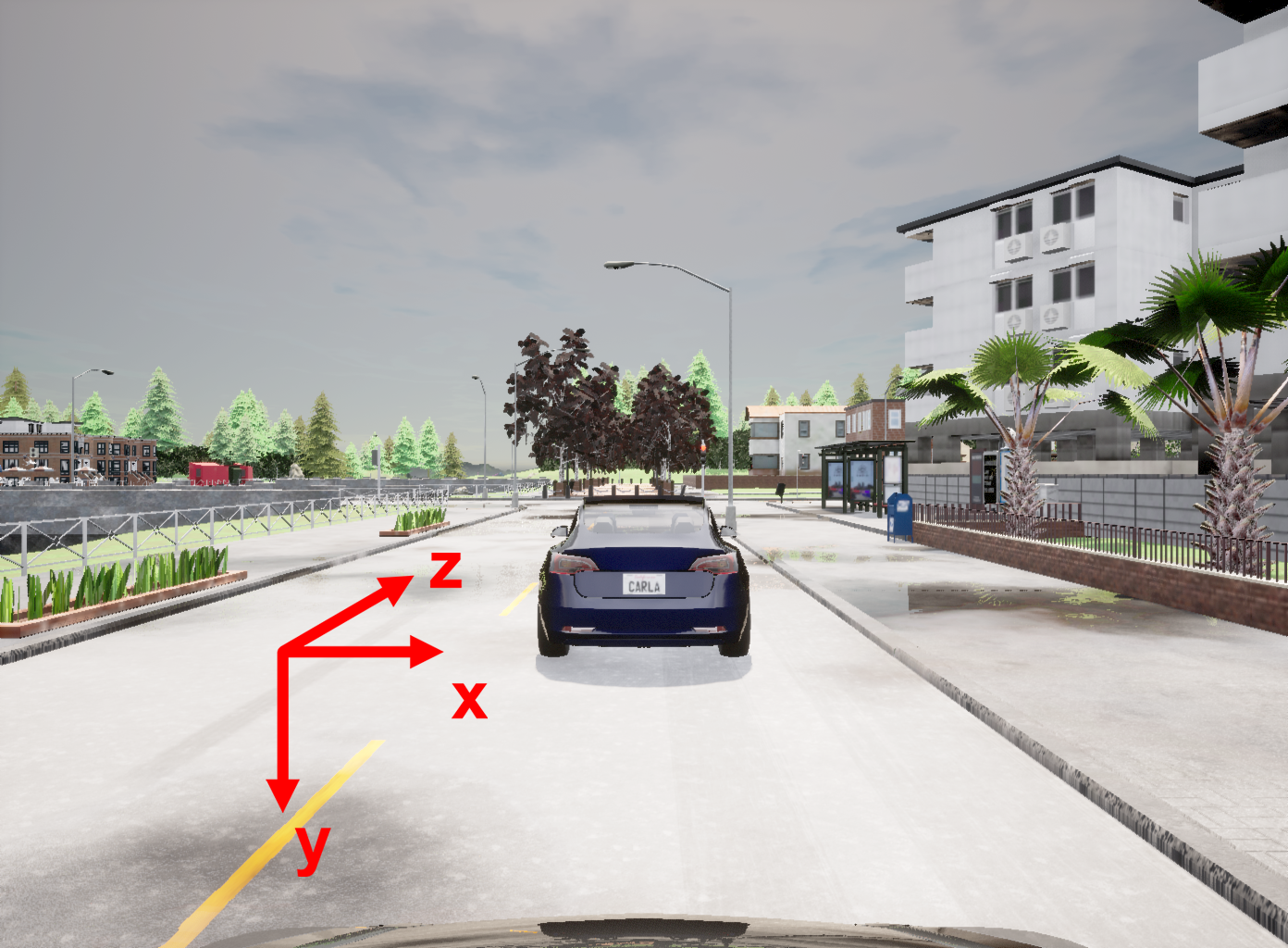
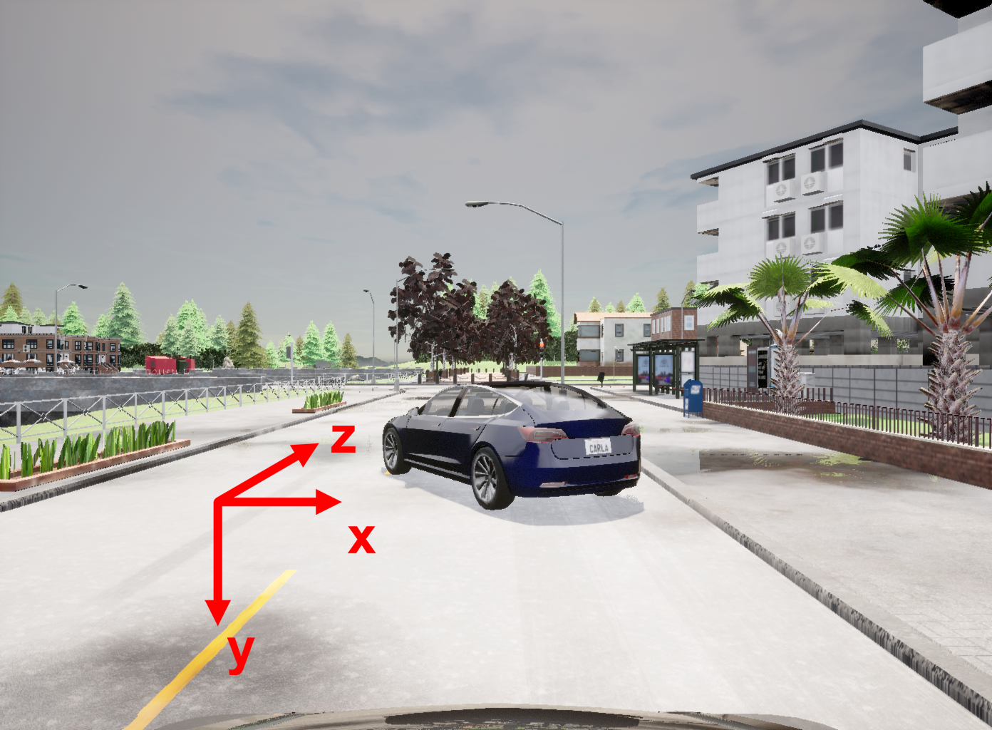
(a) Rotate based on y-axis

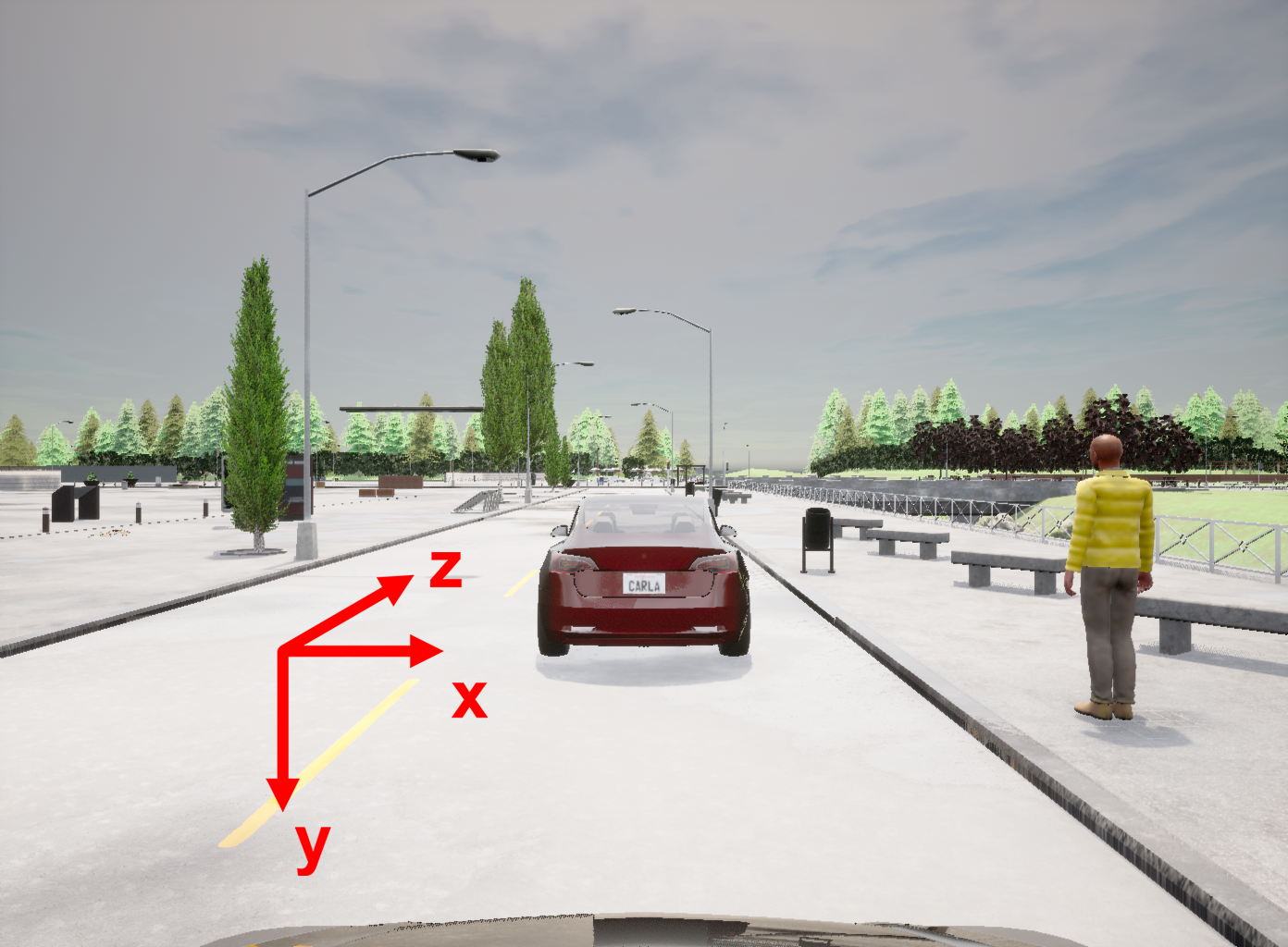
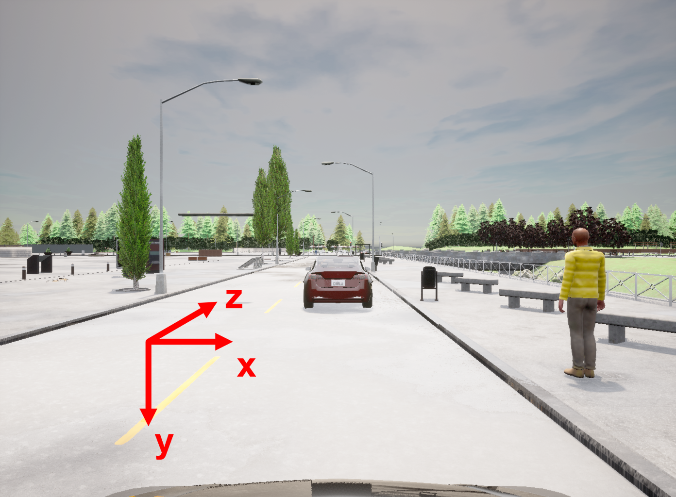
(b) Shift along z-axis

Figure 2: Visualization of the rotation and shifting transformations. The x-axis, y-axis, and z-axis point to the left, down, and forward respectively, while the original point is at the center of the bottom plane for the ego vehicle bounding box.

Fine partition assumption.

For common transformations, we find that when the parameter space is partitioned into tiny subspaces with $\ell_{\infty}$ diameter smaller than some threshold $\tau$, in each subspace bounded by $\ell_{2}$ norm, the distortion incurred by the transformation is upper bounded by the distortion with extreme points as transformation parameter. We formally state such partition assumption and empirically verify it in Appendix A.

Robustness certification goal. Our goal is to certify that, no matter what transformation parameter is chosen by the adversary within a bounded constraint or what transformation strategy is used, the multi-sensor fusion system can always detect the object and locate the object precisely. Here we mainly focus on the task that the multi-sensor fusion system aims to detect the front vehicle when it is present. Extensions to other tasks such as multi-object detection are straightforward via box alignment [7]. Now, we formalize this certification goal by two criteria: Given an input $({\bm{x}},{\bm{p}})$ containing a front vehicle, a transformation $T$, and a constrained parameter space ${\mathcal{S}}$  for any transformed input $(T_{x}({\bm{x}},{\bm{z}}),T_{p}({\bm{p}},{\bm{z}}))$ with ${\bm{z}}\in{\mathcal{S}}$,

• (Detection Certification) the multi-sensor fusion system always outputs a bounding box for the vehicle with confidence $\geq\eta$, where $\eta$ is a pre-defined threshold;

• (IoU Certification) the multi-sensor fusion system always outputs a bounding box for the vehicle whose volume IoU (intersection over union) with the ground-truth bounding box $\geq$ some value $v$.

In the above criteria, $\eta$ determines whether the confidence is high enough to report “vehicle detected”, which is usually set to $0.8$; the IoU is the standard for evaluating bounding box precision (i.e., given two 3D bounding boxes $B_{1},B_{2}\in{\mathcal{B}}$, $\mathrm{IoU}(B_{1},B_{2})=\frac{\mathrm{Vol}(B_{1}\cap B_{2})}{\mathrm{Vol}(B_{1}\cup B_{2})}$ denotes the ratio of intersection volume over the union volume).

3.2 Constructing Certifiably Robust MSFs via Smoothing

Common multi-sensor fusion systems are challenging to be certified due to complex DNN architectures and fusion rules. Hence, we leverage the randomized smoothing [9], in particular, median smoothing [7], as the post-processing protocol to construct a smoothed multi-sensor system. Formally, for each coordinate of the multi-sensor fusion system $g_{i}:{\mathcal{X}}\times{\mathcal{P}}\to\left(({\mathcal{B}}\times{\mathcal{C}}\times[0,1])^{n}\right)_{i}$, we add anisotropic Gaussian noise to the input and define $q$-percentile of the resulting distribution of $g_{i}$:

$$\small{h_{i}}_{q}({\bm{x}},{\bm{p}})=\sup\{y\in\mathbb{R}\ |\ \Pr[g_{i}({\bm{x}}+\delta_{x},{\bm{p}}+\delta_{p})\leq y]\leq q\},$$ (1)

where $\delta_{x}\sim\mathcal{N}(0,\sigma_{x}^{2}{\bm{I}}_{d})$ and $\delta_{p}\sim\mathcal{N}(0,\sigma_{p}^{2}{\bm{I}}_{3\times N})$. We define the resulting smoothed multi-sensor fusion system $h_{q}:=({h_{1}}_{q},{h_{2}}_{q},\dots)$. In practice, we use finite $\delta_{x}$ and $\delta_{p}$ samples to approximate $h_{q}$ by $\hat{h}_{q}$ with high probability and deploy ($q$ is usually set to $0.5$ so it is called median smoothing). For any $q$, we can obtain high-confidence intervals for $h_{q}$ via Monte-Carlo sampling [7].

Though existing work provides robustness certification for smoothed models [9, 7, 26, 8], such certification is limited to single-modal classification or regression against $\ell_{p}$-bounded perturbations. In contrast, our goal is to certify the robustness of multi-sensor fusion systems against semantic transformations under the two aforementioned criteria, where direct applications of prior work are infeasible due to heterogeneous input dimensions, intractable perturbation spaces, and unsupported certification criteria. In the following text, we introduce theoretical results that fulfill our robustness certification goal.

3.3 General Detection Certification

For detection certification, we locate the vehicle bounding box with the highest confidence and consider the confidence of this box as the detection confidence. Hence, for notation simplicity, we let $g:{\mathcal{X}}\times{\mathcal{P}}\to[0,1]$ to represent this detection confidence of the multi-sensor fusion system.

Theorem 3.1.

Let $T=\{T_{x},T_{p}\}$ be a transformation with parameter space $\mathcal{Z}$. Suppose $\mathcal{S}\subseteq\mathcal{Z}$ and $\{\alpha_{i}\}_{i=1}^{M}\subseteq\mathcal{S}$. For detection confidence $g:\mathcal{X}\times\mathcal{P}\to[0,1]$, let $h_{q}({\bm{x}},{\bm{p}})$ be the median smoothing of $g$ as defined in eq. 1. Then for all transformations ${\bm{z}}\in{\mathcal{S}}$, the confidence score of the smoothed detector satisfies:

$$h_{q}(T_{x}({\bm{x}},{\bm{z}}),T_{p}({\bm{p}},{\bm{z}}))\geq\min_{1\leq i\leq M}h_{\underline{q}}(T_{x}({\bm{x}},\alpha_{i}),T_{p}({\bm{p}},\alpha_{i}))$$ (2)

$$\text{where}\quad\underline{q} =\Phi\left(\Phi^{-1}(q)-\sqrt{\frac{M_{x}^{2}}{\sigma_{x}^{2}}+\frac{M_{p}^{2}}{\sigma_{p}^{2}}}\right),$$ (3)

$$M_{x} =\max_{\alpha\in\mathcal{S}}\min_{1\leq i\leq M}\|T_{x}({\bm{x}},\alpha)-T_{x}({\bm{x}},\alpha_{i})\|_{2},\quad M_{p}=\max_{\alpha\in\mathcal{S}}\min_{1\leq i\leq M}\|T_{p}({\bm{p}},\alpha)-T_{p}({\bm{p}},\alpha_{i})\|_{2}.$$ (4)

Remark 3.2.

A full proof for theorem 3.1 is in section B.1. Suppose we have upper bounds for $M_{x}$ and $M_{p}$ (to be given in Lemma 3.3), we can compute a lower bound of $\underline{q}$, and a high-confidence lower bound of $h_{\underline{q}}(T_{x}({\bm{x}},\alpha_{i}),T_{p}({\bm{p}},\alpha_{i}))$ via Monte-Carlo sampling. As a result, we can compute a high-confidence lower bound of detection confidence $h_{q}$. By comparing it with $\eta$ in Section 3.1, we can derive the detection certification.

Lemma 3.3.

If the parameter space to certify ${\mathcal{S}}=[l_{1},u_{1}]\times\cdots\times[l_{m},u_{m}]$ is a hypercube satisfying the finite partition assumption (A.1) with threshold $\tau$, and $\{\alpha_{i}\}_{i=1}^{M}=\{\frac{K_{1}-k_{1}}{K_{1}}l_{1}+\frac{k_{1}}{K_{1}}u_{1}:k_{1}=0,1,\dots,K_{1}\}\times\cdots\times\{\frac{K_{m}-k_{m}}{K_{m}}l_{m}+\frac{k_{m}}{K_{m}}u_{m}:k_{m}=0,1,\dots,K_{m}\}$, where $K_{i}\geq\frac{u_{i}-l_{i}}{\tau}$, then

where $\Delta=\{(k_{1},\dots,k_{m})\in\mathbb{Z}^{m}\ |\ 0\leq k_{i}<K_{i}\}$ and ${\bm{w}}({\bm{k}})=(\frac{K_{1}-k_{1}}{K_{1}}l_{1}+\frac{k_{1}}{K_{1}}u_{1},\cdots,\frac{K_{m}-k_{m}}{K_{m}}l_{m}+\frac{k_{m}}{K_{m}}u_{m})$. $w_{i}=\frac{u_{i}-l_{i}}{K_{i}}{\bm{e}}_{i}$, where ${\bm{e}}_{i}$ is a unit vector at coordinate $i$.

Remark 3.4.

This lemma splits each dimension of ${\mathcal{S}}$ by a $\tau$-cover: $\{\frac{K_{i}-k_{i}}{K_{i}}l_{i}+\frac{k_{i}}{K_{i}}u_{i}:k_{i}=0,1,\dots,K_{i}\}$. Hence, for each tiny subspace defined by $[{\bm{w}}({\bm{k}}),{\bm{w}}({\bm{k}})+(w_{1},\dots,w_{m})]$, we can apply the finite partition assumption (A.1) and the lemma follows. A full proof is in section B.2. The lemma provides feasible upper bounds (via computing maximum of finite terms) for $M_{x}$ and $M_{p}$, so a lower bound of $\underline{q}$ is computable, and hence the robustness certification in Theorem 3.1 is computationally feasible.

3.4 General IoU Certification for 3D Bounding Boxes

Median smoothing for 3D bounding boxes. Given a base 3D bounding box predictor for the front vehicle $g:\mathcal{X}\times\mathcal{P}\to\mathcal{B}$ with $\mathcal{B}\subseteq\mathbb{R}^{6}\times[0,2\pi]$ describing the geometric shape of the bounding box (details in Section 3.1), we denote by $h_{q}({\bm{x}},{\bm{p}})$ the coordinate-wise median smoothing on the outputs of $g$ following Equation 1.

First, by applying Theorem 3.1 on each coordinate of the bounding box from two sides, we obtain the intervals of bounding box coordinates after any possible transformation.

Theorem 3.5.

Let $T=\{T_{x},T_{p}\}$ be a transformation with parameter space $\mathcal{Z}$. Suppose $\mathcal{S}\subseteq\mathcal{Z}$ and $\{\alpha_{i}\}_{i=1}^{N}\subseteq\mathcal{S}$. Let $g_{i}:\mathcal{X}\times\mathcal{P}\to(\mathcal{B})_{i}$ be the $i$-th coordinate of a predicted bounding box of a multi-sensor fusion system, and $h_{iq}({\bm{x}},{\bm{p}})$ be the median smoothing of $g_{i}$ as defined in eq. 1. Then for all transformations $z\in\mathcal{S}$, the $i$-th coordinate of the median smoothed bounding box predictor satisfies:

$$\min_{1\leq i\leq M}h_{i\underline{q}}(T_{x}({\bm{x}},\alpha_{i}),T_{p}({\bm{p}},\alpha_{i})) \leq h_{iq}(T_{x}({\bm{x}},{\bm{z}}),T_{p}({\bm{p}},{\bm{z}}))\leq\max_{1\leq i\leq M}h_{i\overline{q}}(T_{x}({\bm{x}},\alpha_{i}),T_{p}({\bm{p}},\alpha_{i}))$$ (6)

where

$$\underline{q}=\Phi\left(\Phi^{-1}(q)-\sqrt{\frac{M_{x}^{2}}{\sigma_{x}^{2}}+\frac{M_{p}^{2}}{\sigma_{p}^{2}}}\right),\quad\overline{q}=\Phi\left(\Phi^{-1}(q)+\sqrt{\frac{M_{x}^{2}}{\sigma_{x}^{2}}+\frac{M_{p}^{2}}{\sigma_{p}^{2}}}\right).$$ (7)

with $M_{x},M_{p}$ defined as eq. 4.

With the intervals of bounding box coordinates, we propose the following theorem for computing the lower bound of IoU between the output bounding box and the ground truth.

Theorem 3.6.

Let $\mathbf{B}$ be a set of bounding boxes whose coordinates are bounded. We denote the lower bound of each coordinate by $(\underline{x},\underline{y},\underline{z},\underline{w},\underline{h},\underline{l},\underline{r})$ and upper bound by $(\bar{x},\bar{y},\bar{z},\bar{w},\bar{h},\bar{l},\bar{r})$. Let $B_{gt}=(x,y,z,w,h,l,r)$ be the ground truth bounding box. Then for any $B_{i}\in\mathbf{B}$,

$$\mathrm{IoU}(B_{i},B_{gt})\geq\frac{h_{1}\cdot\left(\underline{l}\underline{w}-\mathrm{Vol}(\underline{S}\backslash S_{gt})\right)}{hwl+\bar{h}\bar{w}\bar{l}-h_{2}\cdot\left(\bar{l}\bar{w}-\mathrm{Vol}(\bar{S}\backslash S_{gt})\right)}$$ (8)

where $\underline{S},\bar{S}$ are convex hulls formed by $(\underline{x},\underline{z},\underline{r},\bar{x},\bar{z},\bar{r})$ with respect to $(\underline{w},\underline{l})$ and $(\bar{w},\bar{l})$ (details in section B.3), and $S_{gt}=(x,z,w,l,r)_{gt}$ is the projection of $B_{gt}$ to the $x-z$ plane.

$$h_{1} =\max\big{(}\min_{y^{\prime}\in[\underline{y},\bar{y}]}\min\{h,\underline{h},\frac{h+\underline{h}}{2}-|y^{\prime}-y|\},0\big{)},h_{2}=\max\big{(}\min_{y^{\prime}\in[\underline{y},\bar{y}]}\min\{h,\bar{h},\frac{h+\bar{h}}{2}-|y^{\prime}-y|\},0\big{)}.$$ (9)

Proof Sketch..

To prove a lower bound for the IoU between $B_{i}$ and the ground truth $B_{gt}$, we lower bound the volume of the intersection $B_{i}\cap B_{gt}$ and upper bound the volume of the union $B_{i}\cup B_{gt}$ separately. We estimate the upper bound of union by $\mathrm{Vol}(B_{gt})+\mathrm{Vol}(B_{\max})-\min_{(x,y,z,r)}\mathrm{Vol}(B(x,y,z,\bar{w},\bar{h},\bar{l},r)\cap B_{gt})$. We calculate $h_{1}$ and $h_{2}$ as the smallest possible intersection between $B_{i}$ and $B_{gt}$ along $y$ axis given height $\underline{h}$ and $\bar{h}$, respectively. We then prove the lower bound of their intersection on the $x-z$ plane. We leverage the fact that $\mathrm{Vol}(S\cap S_{gt})=\mathrm{Vol}(S)-\mathrm{Vol}(S\backslash S_{gt})$ and upper bound the volume of $S\backslash S_{gt}$ by considering the convex hull that contains all possible bounding boxes with bounded $(x,z,r)$. The full proof is in Section B.3. ∎

We illustrate the computing procedures for both detection and IoU certification in Appendix C.

3.5 Instantiating Certification for Rotation and Shifting

In this section, we demonstrate how our certification framework works for concrete transformations. Specifically, we discuss two of the most common transformations for vehicles—rotation and shifting. For rotation transformation, we consider a vehicle rotating around the vertical axis based on bounded angle $z$ within a radius $r$, i.e., $z\in[-r,r]$. For shifting transformation, we consider a vehicle moving along the road based on bounded distance $z\in[a,a+2r]$ where $a$ is the original distance.

We instantiate Theorem 3.1 on certifying detection and Theorem 3.6 on certifying IoU against both transformations by computing their interpolation errors $M_{x}$ and $M_{p}$ as defined in Equation 4. We choose $\{\alpha_{i}\}_{i=1}^{K}=\{\frac{2i-K}{K}r\}_{i=1}^{K}$ according to Lemma 3.3 and compute the interpolation errors $M_{x}$ and $M_{p}$ for both transformations. We then leverage $M_{x}$ and $M_{p}$ to derive the lower bound for the detecting confidence score and the IoU regarding the ground-truth bounding box based on Theorems 3.1 and 3.6.

Although the certification procedure can be time-consuming due to space partitioning, the certification cost usually happens before deployment (i.e., pre-deployment verification). After the model is deployed, the inference of smoothed inference is efficient [9]. It is an active field to further reduce the inference cost [20], and our framework can seamlessly integrate these advances.

4 Experimental Evaluation

In this section, we first construct a benchmark for evaluating certified robustness, then systematically evaluate our certification framework COMMIT on several state-of-the-art MSFs.

Dataset. There is no established benchmark for certified robustness evaluation for multi-sensor fusion systems to our knowledge. Hence, we construct a diverse dataset leveraging the CARLA simulator [11]. We consider two types of transformation: 1) Rotation transformation, which is common in the real world since the relative orientation of the car in front of the ego vehicle frequently changes. 2) Shifting transformation, which simulates the scenario where the distance between the front and the ego vehicle changes drastically within a short time.

We provide details of training, testing, and certification data construction as below.

• Training and testing data. We generate our KITTI-CARLA dataset [10] with $5,000$ frames in CARLA Town01 with $50$ pedestrians and $100$ vehicles randomly spawned, in which $3,500$ frames are used for training and $1,500$ frames are used for testing.

• Rotation certification data. We spawn our ego vehicle at 15 spawn points randomly chosen in CARLA Town01, and we then spawn a leading vehicle in front of the ego vehicle within rotation interval $[-30^{\circ},30^{\circ}]$. To study the effect of car color and surrounding objects on the rotation robustness, we collect our rotation certification data with 3 different colors of the leading vehicle in 4 different settings (combination of with or without buildings + with or without pedestrians), which is summarized in Table 3 in Section D.1.

• Shifting certification data. We spawn our ego vehicle at the same 15 spawn points mentioned above and then spawn a leading vehicle facing forward in front of the ego vehicle. We choose $[10,15]$ for the shifting intervals, since according to empirical experiments there is a performance difference among different models at a distance of around 11 meters from the ego vehicle. Similar to the rotation certification data, we use the same environment settings to study the effect of vehicle color, buildings, and pedestrians.

In total, in our benchmark dataset, the certification data contains 62 scenarios for rotation and 62 scenarios for shifting. We set the size of the image input to $64\times 87$ following the standard setting.

Models. We choose two fusion models based on image and point clouds, which are highly ranked on the KITTI leaderboard: FocalsConv [6] and CLOCs [34]. FocalsConv (Voxel R-CNN (Car) + multimodal) achieves 85.22% 3D Average Precision (AP) on the moderate KITTI Car detection task and 100% 3D AP on our KITTI-CARLA dataset. CLOCs (Faster RCNN [38] + SECOND [50]) achieves 80.67% 3D AP on moderate KITTI Car detection task and 100% 3D AP on our KITTI-CARLA dataset.

To compare the performance between fusion models and single-modal models, we select a camera-based model–MonoCon [30], and a LiDAR-based model–SECOND [50], which achieve 19.03% and 78.43% 3D AP respectively on the moderate KITTI Car detection task and 100% on our KITTI-CARLA moderate car detection task.

Metrics. We consider two metrics: detection rate and IoU. In detection certification, attackers aim to reduce the object detection confidence score to fool the detectors to detect nothing. We aim to certify the lower bound of the detection rate under a detection threshold, where Det@80 means the ratio of detected bounding boxes with confidence score larger than 0.8. In IoU certification, we aim to lower bound the IoU between the detected bounding box and the ground truth bounding box when attackers are allowed to attack the IoU in a transformation space. As for the notation in all tables, AP@50 means the ratio of detected bounding boxes whose IoU with the ground truth bounding boxes is larger than 0.5. In Figure 3 and Figure 7, we show corresponding results by choosing different detection or IoU thresholds.

Certification Details. To make the models adapt with Gaussian noise smoothed data, we train two sets of models with Gaussian augmentation [9] using noise variance $\sigma=0.25$ and $\sigma=0.5$. For the ease of robustness certification, for rotation certification, we use models trained with $\sigma=0.25$ to construct smoothed models; for shifting certification, we use models trained with $\sigma=0.5$. Note that our framework allows using different $\sigma$ and sample strategies for image and point cloud data.

Table 1: Certified and empirical robustness of different models against different semantic transformations. Each row represents the corresponding model and attack radius. “Benign”, “Adv (Vanilla)”, “Adv (Smoothed)”, and “Certification” stand for benign performance, vanilla models’ performance under attacks, smoothed models’ performance under attacks, and certified lower bound of performance under bounded transformations. Det@80 and AP@50 mean that we use 0.8 and 0.5 as the thresholds of confidence score and IoU score. Results under other thresholds are in Section D.2.

(a) Rotation

Model	Input	Attack Radius	Benign		Adv (Vanilla)		Adv (Smoothed)		Certification
	Modality		Det@80	AP@50	Det@80	AP@50	Det@80	AP@50	Det@80	AP@50
MonoCon [30]	Image	$|r|\leq 10^{\circ}$	100.00%	100.00%	58.06%	56.45%	80.65%	82.26%	75.81%	0.00%
		$|r|\leq 15^{\circ}$			58.06%	54.84%	80.65%	82.26%	75.81%	0.00%
		$|r|\leq 20^{\circ}$			58.06%	53.23%	80.65%	74.19%	75.81%	0.00%
		$|r|\leq 25^{\circ}$			45.16%	35.48%	80.65%	16.13%	75.81%	0.00%
		$|r|\leq 30^{\circ}$			32.26%	0.00%	80.65%	3.23%	75.81%	0.00%
SECOND [50]	Point Cloud	$|r|\leq 10^{\circ}$	100.00%	100.00%	19.35%	96.77%	0.00%	100.00%	0.00%	100.00%
		$|r|\leq 15^{\circ}$			19.35%	96.77%	0.00%	100.00%	0.00%	100.00%
		$|r|\leq 20^{\circ}$			19.35%	96.77%	0.00%	100.00%	0.00%	100.00%
		$|r|\leq 25^{\circ}$			1.61%	83.87%	0.00%	96.77%	0.00%	0.00%
		$|r|\leq 30^{\circ}$			1.61%	51.61%	0.00%	54.84%	0.00%	0.00%
CLOCs [34]	Image + Point Cloud	$|r|\leq 10^{\circ}$	100.00%	100.00%	100.00%	90.32%	88.71%	100.00%	88.71%	100.00%
		$|r|\leq 15^{\circ}$			100.00%	90.32%	66.13%	98.39%	66.13%	87.10%
		$|r|\leq 20^{\circ}$			100.00%	88.71%	50.00%	98.39%	50.00%	69.35%
		$|r|\leq 25^{\circ}$			20.97%	87.10%	50.00%	98.39%	50.00%	67.74%
		$|r|\leq 30^{\circ}$			3.23%	80.65%	50.00%	98.39%	50.00%	53.23%
FocalsConv [6]	Image + Point Cloud	$|r|\leq 10^{\circ}$	100.00%	100.00%	100.00%	96.77%	100.00%	100.00%	100.00%	0.00%
		$|r|\leq 15^{\circ}$			100.00%	0.00%	100.00%	0.00%	100.00%	0.00%
		$|r|\leq 20^{\circ}$			100.00%	0.00%	100.00%	0.00%	100.00%	0.00%
		$|r|\leq 25^{\circ}$			100.00%	0.00%	100.00%	0.00%	100.00%	0.00%
		$|r|\leq 30^{\circ}$			98.39%	0.00%	100.00%	0.00%	100.00%	0.00%

(b) Shifting

Model	Input	Attack Radius	Benign		Adv (Vanilla)		Adv (Smoothed)		Certification
	Modality		Det@80	AP@50	Det@80	AP@50	Det@80	AP@50	Det@80	AP@50
MonoCon [30]	Image	$10\leq z\leq 11$	100.00%	100.00%	66.13%	77.42%	66.13%	77.42%	64.52%	41.94%
		$10\leq z\leq 12$			62.90%	74.19%	62.90%	74.19%	61.29%	1.61%
		$10\leq z\leq 13$			56.45%	72.58%	56.45%	72.58%	51.61%	0.00%
		$10\leq z\leq 14$			46.77%	33.87%	46.77%	33.87%	41.94%	0.00%
		$10\leq z\leq 15$			27.42%	1.61%	27.42%	1.61%	27.42%	0.00%
SECOND [50]	Point Cloud	$10\leq z\leq 11$	100.00%	100.00%	0.00%	93.55%	0.00%	100.00%	0.00%	0.00%
		$10\leq z\leq 12$			0.00%	80.65%	0.00%	80.65%	0.00%	0.00%
		$10\leq z\leq 13$			0.00%	80.65%	0.00%	80.65%	0.00%	0.00%
		$10\leq z\leq 14$			0.00%	80.65%	0.00%	80.65%	0.00%	0.00%
		$10\leq z\leq 15$			0.00%	80.65%	0.00%	80.65%	0.00%	0.00%
CLOCs [34]	Image + Point Cloud	$10\leq z\leq 11$	100.00%	100.00%	100.00%	93.55%	93.55%	100.00%	67.74%	79.03%
		$10\leq z\leq 12$			100.00%	80.65%	93.55%	80.65%	66.13%	51.61%
		$10\leq z\leq 13$			85.48%	80.65%	88.71%	80.65%	64.52%	48.39%
		$10\leq z\leq 14$			64.52%	80.65%	85.48%	80.65%	62.90%	48.39%
		$10\leq z\leq 15$			64.52%	80.65%	83.87%	80.65%	61.29%	48.39%
FocalsConv [6]	Image + Point Cloud	$10\leq z\leq 11$	100.00%	100.00%	96.77%	0.00%	96.77%	100.00%	54.84%	0.00%
		$10\leq z\leq 12$			96.77%	0.00%	96.77%	100.00%	4.84%	0.00%
		$10\leq z\leq 13$			0.00%	0.00%	0.00%	82.26%	0.00%	0.00%
		$10\leq z\leq 14$			0.00%	0.00%	0.00%	14.52%	0.00%	0.00%
		$10\leq z\leq 15$			0.00%	0.00%	0.00%	8.06%	0.00%	0.00%

4.1 Certification against Rotation Transformation

In this section, we present the evaluations for the certified and empirical results of our framework COMMIT against rotation transformation. In terms of certification, we use small intervals of rotation angles $0.1^{\circ}$ and samples 1000 times with $\sigma_{x}=0.25,\sigma_{p}=0.25$ Gaussian noises for each interval (in total $600\times 1000$ Gaussian noises with certification confidence 95%) to estimate $h_{q}$ (see definition in Section 3.2). Empirically, we split the rotation intervals into small $0.01^{\circ}$ and use the models’ worst empirical performance in these samples as the empirical robustness against rotation attacks, which is equivalent to the PGD attack with step $0.01^{\circ}$. We set the overall confidence of certification to be $95\%$, aligning with the setting in [23].

	$|r|\leq 10^{\circ}$	$|r|\leq 15^{\circ}$	$|r|\leq 20^{\circ}$	$|r|\leq 25^{\circ}$	$|r|\leq 30^{\circ}$
Detection
	$\text{TH}_{\text{conf}}$	$\text{TH}_{\text{conf}}$	$\text{TH}_{\text{conf}}$	$\text{TH}_{\text{conf}}$	$\text{TH}_{\text{conf}}$
IoU
	$\text{TH}_{\text{IoU}}$	$\text{TH}_{\text{IoU}}$	$\text{TH}_{\text{IoU}}$	$\text{TH}_{\text{IoU}}$	$\text{TH}_{\text{IoU}}$

Figure 3: Certified and empirical robustness on detection rate and IoU against rotation transformation (smoothing $\sigma=0.25$) under different thresholds. Solid lines represent the certified bounds, and dashed lines show the empirical performance under PGD attacks. $x$-axis represents the threshold for confidence score ($\text{TH}_{\text{conf}}$) and IoU score ($\text{TH}_{\text{IoU}}$), and $y$-axis represents the ratio of detection whose confidence / IoU score is larger than the confidence / IoU threshold.

Table 1(a) shows the results in the $[-30^{\circ},30^{\circ}]$ rotation interval. We can see that in terms of detection ability, the robustness order is $\text{FocalsConv}>\text{MonoCon}>\text{CLOCs}>\text{SECOND}$, according to both the empirical and certification results. Hence, FocalsConv and MonoCon may be more likely to predict the existence of the object when it exists. Furthermore, we observe that multi-sensor fusion models have better detection robustness compared with single-modal models under the same threshold (e.g., $\text{FocalsConv}>\text{MonoCon},\text{CLOCs}>\text{SECOND}$). In addition, we find that our certification is pretty tight in many cases. In particular, row “Certification" serves as the lower bound of row “Adv (Smoothed)", and in most cases they are very close, indicating the tight robustness certification.

Now we study the IoU metric since we expect that models can predict not only with high confidence but also precise bounding boxes. By comparing the empirical and certified results in IoU metric, CLOCs outperforms all other models. It is easy to understand that CLOCs outperforms single-modal models since it combines the information from both images and point clouds. However, FocalsConv is not as robust as CLOCs even though it is a also camera-LiDAR fusion model, which could be due to the fusion mechanism, and thus more robust fusion algorithms will help improve the model prediction robustness.

We also present some interesting findings of rotation transformation in Section D.2 (e.g., the effect of threshold, the effect of attack radius) and possible reasons for detection failure cases in rotation transformation in Section D.5.

4.2 Certification against Shifting Transformation

Here we present the evaluations for the certified and empirical results of our framework COMMIT against shifting transformation. In terms of the robustness certification, we use small shifting intervals of size 0.01 and samples 1000 times with $\sigma_{x}=0.5,\sigma_{p}=0.5$ Gaussian noises in each interval to estimate $h_{q}$ (see definition in Section 3.2). In the empirical experiments, we divide the shifting intervals into small intervals of size 0.001 and use the worst empirical performance of the model among these samples as the empirical robustness against PGD attacks. We set the overall confidence of certification to be $95\%$ following the standard setting.

Table 1(b) shows the certified and empirical robustness of different models against shifting transformation. The robustness in terms of both detection ability and IoU is $\text{CLOCs}>\text{SECOND}\approx\text{MonoCon}>\text{FocalsConv}$. We also notice that SECOND outperforms MonoCon when the distance is larger while they have a similar performance within short distances, which could be due to the accurate estimation of large distances by LiDAR sensors and the lack of depth information in the 2D camera images. However, this does not mean that image data do not have meaningful features because CLOCs is always more robust than SECOND, which could be caused by the fact that more candidates are proposed by 2D detectors (Faster RCNN in our case) which are ignored by the point cloud detectors. On the other hand, there is an interesting finding that FocalsConv performs poorly against shifting transformation. The reason might be that FocalsConv highly depends on the image features, and shifting transformation can attack the image and point cloud spaces at the same time. This implies that the design of the fusion mechanism is also an important factor on the robustness of multi-modal sensor fusion models.

We also present some interesting findings under shifting transformation in Section D.2 (e.g., the effects of threshold, the effect of attack radius) and possible reasons for detection failure cases in shifting transformation in Section D.5.

5 Conclusion

In this work we provide the first robustness certification framework COMMIT for multi-sensor fusion systems against semantic transformations based on different criteria. Our theoretical certification framework is flexible for different models and transformations. Our evaluations show that current fusion models are more robust than single-modal models, and the design of the fusion mechanism is an important factor in improving the robustness against semantic transformations.

The appendices are organized as follows:

• In Appendix A, we formally present the finite partition assumption (from Section 3.1) and provide an empirical verification of the assumption.

• In Appendix B, we present the detailed proofs for lemmas and theorems in Sections 3.3 and 3.4 of the main paper.

• In Appendix C, we present some additional details of our two certification strategies: Section C.1 for certifying the detection rate, and Section C.2 for certifying the IoU between the detection and the ground truth. We include the detailed algorithm description and the complete pseudocode for each algorithm. We will make our implementation public upon acceptance.

• In Appendix D, we show dataset details (Section D.1), detailed experimental evaluation (Section D.2), some ablation studies on sample strategies (Section D.3) and smoothing parameter $\sigma$ (Section D.4), and failure case analysis (Section D.5).

Appendix A Details of Fine Partition Assumption

As introduced in Section 3.1, we impose the following assumption for the transformation.

Assumption A.1.

For given transformation $T=\{T_{x},T_{p}\}$ with parameter space ${\mathcal{Z}}\subseteq{\mathbb{R}}^{m}$, there exists a small threshold $\tau>0$, for any polytope of the parameter space ${\mathcal{Z}}_{\mathrm{sub}}\subseteq{\mathcal{Z}}$ whose $\ell_{\infty}$ diameter is smaller than $\tau$, i.e., $\mathrm{diam}_{\infty}({\mathcal{Z}}_{\mathrm{sub}})<\tau$, when parameters are picked from the subspace, the pairwise $\ell_{2}$ distance between transformed outputs is upper bounded by maximum pairwise $\ell_{2}$ distance with extreme points picked as parameters. Formally, let $E({\mathcal{Z}}_{\mathrm{sub}})$ be the set of extreme points of ${\mathcal{Z}}_{\mathrm{sub}}$, then $\forall{\bm{z}}_{1},{\bm{z}}_{2}\in{\mathcal{Z}}_{\mathrm{sub}},{\bm{x}}\in{\mathcal{X}},{\bm{p}}\in{\mathcal{P}}$,

$$\|T_{x}({\bm{x}},{\bm{z}}_{1})-T_{x}({\bm{x}},{\bm{z}}_{2})\|_{2}\leq\max_{{\bm{z}}^{\prime}_{1},{\bm{z}}^{\prime}_{2}\in E({\mathcal{Z}}_{\mathrm{sub}})}\|T_{x}({\bm{x}},{\bm{z}}^{\prime}_{1})-T_{x}({\bm{x}},{\bm{z}}^{\prime}_{2})\|_{2},$$ (10)

$$\|T_{p}({\bm{p}},{\bm{z}}_{1})-T_{p}({\bm{p}},{\bm{z}}_{2})\|_{2}\leq\max_{{\bm{z}}^{\prime}_{1},{\bm{z}}^{\prime}_{2}\in E({\mathcal{Z}}_{\mathrm{sub}})}\|T_{p}({\bm{p}},{\bm{z}}^{\prime}_{1})-T_{p}({\bm{p}},{\bm{z}}^{\prime}_{2})\|_{2}.$$

Remark A.2.

Intuitively, the assumption states that, within a tiny subspace of the parameter space, the displacement incurred by the transformation, when measured by Euclidean distance, is proportional to the magnitude between parameters, so the maximum displacement can be upper bounded by the displacement incurred by choosing extreme points as the transformation parameters. Taking the rotation as an example, within a sufficiently small range of rotation angle $[r-\Delta,r+\Delta]$ where $2\Delta<\tau$, the assumption means that, the difference between rotated images $\|T_{x}({\bm{x}},\delta_{1})-T_{x}({\bm{x}},\delta_{2})\|_{2}$ and point clouds $\|T_{p}({\bm{p}},\delta_{1})-T_{p}({\bm{p}},\delta_{2})\|_{2}$ is no larger than $\|T_{x}({\bm{x}},r-\Delta)-T_{x}({\bm{x}},r+\Delta)\|_{2}$ and $\|T_{p}({\bm{p}},r-\Delta)-T_{p}({\bm{p}},r+\Delta)\|_{2}$ respectively.

While it is hard to prove the A.1, we empirically evaluate the A.1 by plotting the distribution of image $\ell_{2}$ norm with different interval sizes ($0.001^{\circ},0.01^{\circ},0.02^{\circ},0.03^{\circ},0.04^{\circ},0.05^{\circ}$ for rotation and $0.001,0.01,0.02,0.03,0.04,0.05$ for shifting) in randomly selected big intervals ($0.06^{\circ}$ for rotation and 0.07 for shifting) in Figure 4.

From Table 3(a) and Table 3(b), we can notice that with larger rotation and shifting intervals, the image $\ell_{2}$ norm becomes larger and larger, and the $\ell_{2}$ distance between the endpoints of each big interval can bound the $\ell_{2}$ distance between randomly chosen points in that big interval, which means that the pairwise $\ell_{2}$ distance picks the maximum value with extreme points when the transformation intervals are sufficiently small, and thus A.1 is empirically confirmed.

$\ell_{2}$ norm
	Interval size	Interval size	Interval size	Interval size	Interval size	Interval size

(a) Image $\ell_{2}$ norm distribution in rotation transformation.

$\ell_{2}$ norm
	Interval size	Interval size	Interval size	Interval size	Interval size	Interval size

(b) Image $\ell_{2}$ norm distribution in shifting transformation.

Figure 4: Image $\ell_{2}$ norm distribution in rotation and shift transformation. Images are from spawn point 15, 30, 43, 46, 57 and 86 from dataset with building and without pedestrian. The scatter plots show the $\ell_{2}$ distance of randomly chosen pairs in randomly chosen big intervals. The black line is the $\ell_{2}$ distance between the endpoints of big intervals.

Appendix B Proofs

B.1 Proof of theorem 3.1: Detection Certification

In this section, we present the full proof of theorem 3.1, which provides generic certification for multi-sensor fusion detection against an abstract transformation. We first restate this theorem from the main text.

Theorem 3.1 (restated).

Let $T=\{T_{x},T_{p}\}$ be a transformation with parameter space $\mathcal{Z}$. Suppose $\mathcal{S}\subseteq\mathcal{Z}$ and $\{\alpha_{i}\}_{i=1}^{M}\subseteq\mathcal{S}$. For detection confidence $g:\mathcal{X}\times\mathcal{P}\to[0,1]$, let $h_{q}({\bm{x}},{\bm{p}})$ be the median smoothing of $g$ as defined in eq. 1. Then for all transformations ${\bm{z}}\in{\mathcal{S}}$, the confidence score of the median smoothed detector satisfies:

$$h_{q}(T_{x}({\bm{x}},{\bm{z}}),T_{p}({\bm{p}},{\bm{z}}))\geq\min_{1\leq i\leq M}h_{\underline{q}}(T_{x}({\bm{x}},\alpha_{i}),T_{p}({\bm{p}},\alpha_{i}))$$ (11)

where

$$\underline{q} =\Phi\left(\Phi^{-1}(q)-\sqrt{\frac{M_{x}^{2}}{\sigma_{x}^{2}}+\frac{M_{p}^{2}}{\sigma_{p}^{2}}}\right),$$ (12)

$$M_{x} =\max_{\alpha\in\mathcal{S}}\min_{1\leq i\leq M}\|T_{x}({\bm{x}},\alpha)-T_{x}({\bm{x}},\alpha_{i})\|_{2},$$ (13)

$$M_{p} =\max_{\alpha\in\mathcal{S}}\min_{1\leq i\leq M}\|T_{p}({\bm{p}},\alpha)-T_{p}({\bm{p}},\alpha_{i})\|_{2}.$$ (14)

Proof.

We first recall the median smoothed classifier $h_{q}({\bm{x}},{\bm{p}})=\sup\{y\in\mathbb{R}\ |\ \Pr[g({\bm{x}}+\delta_{x},{\bm{p}}+\delta_{p})\leq y]\leq q\}$, where $\delta_{x}\sim{\mathcal{N}}(0,\sigma_{x}^{2}\mathbf{I}_{d})$ and $\delta_{p}\sim{\mathcal{N}}(0,\sigma^{2}_{p}\mathbf{I}_{3\times N})$.

Consider a function $f:\mathbb{R}^{d}\times\mathbb{R}^{3\times N}\to[0,1]$ with $f({\bm{x}},{\bm{p}})=\Pr[g({\bm{x}}+\delta_{x},{\bm{p}}+\delta_{p})\leq h_{\underline{q}}({\bm{x}},{\bm{p}})]$. We define $\tilde{g}:{\mathcal{X}}\times{\mathcal{P}}\to[0,1]$ as $\tilde{g}({\bm{x}},{\bm{p}})=g({\bm{x}},\frac{\sigma_{p}}{\sigma_{x}}{\bm{p}})$. Then

$$f({\bm{x}},{\bm{p}})=\Pr[\tilde{g}({\bm{x}}+\delta_{x},{\bm{p}}^{\prime}+\delta_{p}^{\prime})\leq h_{\underline{q}}({\bm{x}},{\bm{p}})],\ \text{where}\ {\bm{p}}^{\prime}=\frac{\sigma_{x}}{\sigma_{p}}{\bm{p}},\ \delta_{p}^{\prime}\sim{\mathcal{N}}(0,\sigma_{x}^{2}\mathbf{I}_{3\times N}).$$ (15)

We now introduce a lemma from [39](Lemma 2) and [7](Corollary 1).

Lemma B.1.

For any $g:\mathbb{R}^{d}\to[l,u]$, let $f(x)=\mathbb{E}[g(x+G)]$ where $G\sim{\mathcal{N}}(0,\sigma^{2}\mathbf{I})$. Then the map $\eta(x)=\sigma\cdot\Phi^{-1}(\frac{f(x)-l}{u-l})$ is 1-Lipschitz.

Note that $f({\bm{x}},{\bm{p}}^{\prime})=\mathbb{E}\left(\mathbbm{1}[\tilde{g}({\bm{x}}+\delta_{x},{\bm{p}}^{\prime}+\delta_{p}^{\prime})\leq h_{\underline{q}}({\bm{x}},{\bm{p}})]\right)$, which means $\sigma_{x}\cdot\Phi^{-1}(f({\bm{x}},{\bm{p}}^{\prime}))$ is 1-Lipschitz.

Now let us consider an arbitrary transformation ${\bm{z}}\in{\mathcal{S}}$, by the definition of $M_{x}$ and $M_{p}$ we have

$$\forall{\bm{z}}\in{\mathcal{S}},\ \exists\alpha_{i},\ \|T_{x}({\bm{x}},{\bm{z}})-T_{x}({\bm{x}},\alpha_{i})\|_{2}\leq M_{x},\|T_{p}({\bm{p}},{\bm{z}})-T_{p}({\bm{p}},\alpha_{i})\|_{2}\leq M_{p}.$$ (16)

Then

$$\sigma_{x} \Phi^{-1}\Big{(}\Pr\Big{[}g(T_{x}({\bm{x}},{\bm{z}})+\delta_{x},T_{p}({\bm{p}},{\bm{z}})+\delta_{p})\leq h_{\underline{q}}({\bm{x}},{\bm{p}})\Big{]}\Big{)}=\sigma_{x}\Phi^{-1}\left(f(T_{x}({\bm{x}},{\bm{z}}),\frac{\sigma_{x}}{\sigma_{p}}T_{p}({\bm{p}},{\bm{z}}))\right)$$ (17)

$$\geq\sigma_{x}\Phi^{-1}\left(f\Big{(}T_{x}({\bm{x}},\alpha_{i}),\frac{\sigma_{x}}{\sigma_{p}}T_{p}({\bm{p}},\alpha_{i})\Big{)}\right)-\sqrt{M_{x}^{2}+\frac{\sigma_{x}^{2}}{\sigma_{p}^{2}}M_{p}^{2}}$$ (18)

$$\geq\sigma_{x}\Phi^{-1}\Big{(}\Pr\Big{[}g(T_{x}({\bm{x}},\alpha_{i})+\delta_{x},T_{p}({\bm{p}},\alpha_{i})+\delta_{p})\leq h_{\underline{q}}({\bm{x}},{\bm{p}})\Big{]}\Big{)}-\sqrt{M_{x}^{2}+\frac{\sigma_{x}^{2}}{\sigma_{p}^{2}}M_{p}^{2}}$$ (19)

$$=\sigma_{x}\Phi^{-1}(\underline{q})-\sqrt{M_{x}^{2}+\frac{\sigma_{x}^{2}}{\sigma_{p}^{2}}M_{p}^{2}}$$ (20)

$$=\sigma_{x}\Phi^{-1}(q).$$ (21)

Since that $\Phi(\cdot)$ is monotonic, we conclude that

$$\forall{\bm{z}}\in{\mathcal{S}},\ \exists\alpha_{i},\mathrm{s.t.}\ h_{q}(T_{x}({\bm{x}},{\bm{z}}),T_{p}({\bm{p}},{\bm{z}}))\geq h_{\underline{q}}({\bm{x}},{\bm{p}}).$$ (22)

∎

B.2 Proof of lemma 3.3: Upper Bound for the Interpolation Error

Lemma 3.3 (restated).

If the parameter space to certify ${\mathcal{S}}=[l_{1},u_{1}]\times\cdots\times[l_{m},u_{m}]$ is a hypercube satisfying A.1 with threshold $\tau$, and $\{\alpha_{i}\}_{i=1}^{M}=\{\frac{K_{1}-k_{1}}{K_{1}}l_{1}+\frac{k_{1}}{K_{1}}u_{1}:k_{1}=0,1,\dots,K_{1}\}\times\cdots\times\{\frac{K_{m}-k_{m}}{K_{m}}l_{m}+\frac{k_{m}}{K_{m}}u_{m}:k_{m}=0,1,\dots,K_{m}\}$, where $K_{i}\geq\frac{u_{i}-l_{i}}{\tau}$, then

$$M_{x} \leq\sum_{i=1}^{m}\max_{{\bm{k}}\in\Delta}\Big{\|}T_{x}({\bm{x}},{\bm{w}}({\bm{k}}))-T_{x}({\bm{x}},{\bm{w}}({\bm{k}})+w_{i})\Big{\|}_{2},$$ (23)

$$M_{p} \leq\sum_{i=1}^{m}\max_{{\bm{k}}\in\Delta}\Big{\|}T_{p}({\bm{p}},{\bm{w}}({\bm{k}}))-T_{p}({\bm{p}},{\bm{w}}({\bm{k}})+w_{i})\Big{\|}_{2}$$ (24)

where $\Delta=\{(k_{1},\dots,k_{m})\in\mathbb{Z}^{m}\ |\ 0\leq k_{i}<K_{i}\}$ and ${\bm{w}}({\bm{k}})=(\frac{K_{1}-k_{1}}{K_{1}}l_{1}+\frac{k_{1}}{K_{1}}u_{1},\cdots,\frac{K_{m}-k_{m}}{K_{m}}l_{m}+\frac{k_{m}}{K_{m}}u_{m})$. $w_{i}=\frac{u_{i}-l_{i}}{K_{i}}{\bm{e}}_{i}$, where ${\bm{e}}_{i}$ is a unit vector at coordinate $i$.

Proof.

Let ${\bm{z}}\in{\mathcal{S}}\subseteq\mathbb{R}^{m}$ be a parameter in the parameter space to certify and ${\bm{z}}=(z_{1},\dots,z_{m})$. There must be $(k_{1},k_{2},\dots,k_{m})$ with $k_{i}\in\{0,1,\dots,K_{i}-1\}$, such that

$$\frac{K_{i}-k_{i}}{K_{i}}l_{i}+\frac{k_{i}}{K_{i}}u_{i}\leq z_{i}\leq\frac{K_{i}-k_{i}-1}{K_{i}}l_{i}+\frac{k_{i}+1}{K_{i}}u_{i},\ \forall i=1,2,\dots,m.$$ (25)

Let ${\bm{k}}=(k_{1},k_{2},\dots,k_{m})$. Consider the small polytope ${\mathcal{Z}}_{\mathrm{sub}}={\bm{k}}+[0,1]^{m}\cdot(w_{1},\dots,w_{m})$. By A.1,

$$\|T_{x}({\bm{x}},{\bm{z}})-T_{x}({\bm{x}},{\bm{w}}(k))\|_{2} \leq\max_{\alpha,\beta\in E({\mathcal{Z}}_{\mathrm{sub}})}\|T_{x}({\bm{x}},\alpha)-T_{x}({\bm{x}},\beta)\|_{2}$$ (26)

$$=\|T_{x}({\bm{x}},{\bm{z}}_{1})-T_{x}({\bm{x}},{\bm{z}}_{2})\|_{2}$$ (27)

where ${\bm{z}}_{1}={\bm{k}}+I_{1}\cdot(w_{1},\dots,w_{m})$ and ${\bm{z}}_{2}={\bm{k}}+I_{2}\cdot(w_{1},\dots,w_{m})$ for some $I_{1},I_{2}\in\{0,1\}^{m}$. Let $\{\alpha_{1},\alpha_{2},\dots,\alpha_{n}\}$ be a shortest path from ${\bm{z}}_{1}$ to ${\bm{z}}_{2}$ such that $\alpha_{i}\in\{0,1\}^{m}\cdot(w_{1},\dots,w_{m})+{\bm{k}}$, $\alpha_{1}={\bm{k}}_{1}$, and $\alpha_{n}={\bm{k}}_{2}$. Moreover, $\alpha_{j}$ and $\alpha_{j+1}$ differ on exactly 1 non-repeating coordinate $c_{j}$. Then

$$\|T_{x}({\bm{x}},{\bm{z}}_{1})-T_{x}({\bm{x}},{\bm{z}}_{2})\|_{2} =\|\sum_{j=1}^{n-1}T_{x}({\bm{x}},\alpha_{j})-T_{x}(x,\alpha_{j+1})\|_{2}$$ (28)

$$\leq\sum_{j=1}^{n-1}\|T_{x}({\bm{x}},\alpha_{j})-T_{x}({\bm{x}},\alpha_{j+1})\|_{2}$$ (29)

$$\leq\sum_{j=1}^{n-1}\max_{{\bm{k}}\in\Delta}\|T_{x}({\bm{x}},{\bm{w}}({\bm{k}}))-T_{x}({\bm{x}},{\bm{w}}({\bm{k}})+w_{c_{j}})\|_{2},$$ (30)

$$\leq\sum_{i=1}^{m}\max_{{\bm{k}}\in\Delta}\|T_{x}({\bm{x}},{\bm{w}}({\bm{k}}))-T_{x}({\bm{x}},{\bm{w}}({\bm{k}})+w_{i})\|_{2}.$$ (31)

which implies eq. 23. eq. 24 also holds, following exactly the same argument for point clouds. ∎

B.3 Proof of theorem 3.6: General IoU Certification for 3D Bounding Boxes

We first recall theorem 3.6 from the main paper. Note that we omit details for the convex hulls $\underline{S},\bar{S}$ in the main paper version for simplicity. Here we provide a complete version with a formal description for $\underline{S},\bar{S}$.

Theorem 3.6 (restated).

Let $\mathbf{B}$ be a set of bounding boxes whose coordinates are bounded. We denote the lower bound of each coordinate by $(\underline{x},\underline{y},\underline{z},\underline{w},\underline{h},\underline{l},\underline{r})$ and upper bound by $(\bar{x},\bar{y},\bar{z},\bar{w},\bar{h},\bar{l},\bar{r})$. Let $B_{gt}=(x,y,z,w,h,l,r)$ be the ground truth bounding box. Then for any $B_{i}\in\mathbf{B}$,

$$\mathrm{IoU}(B_{i},B_{gt})\geq\frac{h_{1}\cdot\left(\underline{l}\underline{w}-\mathrm{Vol}(\underline{S}\backslash S_{gt})\right)}{hwl+\bar{h}\bar{w}\bar{l}-h_{2}\cdot\left(\bar{l}\bar{w}-\mathrm{Vol}(\bar{S}\backslash S_{gt})\right)}$$ (32)

where $S_{gt}=(x,z,w,l,r)_{gt}$ is the projection of $B_{gt}$ to the $x-z$ plane.

$$h_{1} =\max\big{(}\min_{y^{\prime}\in[\underline{y},\bar{y}]}\min\{h,\underline{h},\frac{h+\underline{h}}{2}-|y^{\prime}-y|\},0\big{)},$$

$$h_{2} =\max\big{(}\min_{y^{\prime}\in[\underline{y},\bar{y}]}\min\{h,\bar{h},\frac{h+\bar{h}}{2}-|y^{\prime}-y|\},0\big{)}.$$ (33)

$\underline{S},\bar{S}$ are convex hulls formed by $(\underline{x},\underline{z},\underline{r},\bar{x},\bar{z},\bar{r})$ with respect to $(\underline{w},\underline{l})$ and $(\bar{w},\bar{l})$. Here we formally define $C(\underline{x},\underline{z},\underline{r},\bar{x},\bar{z},\bar{r},w,l)$. Let $\varphi=\arctan(\frac{l}{w})$, we first define

$$\Delta x_{\max,k} =\max_{\theta\in[\underline{r},\bar{r}]}\sqrt{w^{2}+l^{2}}\cos(\theta+k\varphi),$$ (34)

$$\Delta x_{\min,k} =\min_{\theta\in[\underline{r},\bar{r}]}\sqrt{w^{2}+l^{2}}\cos(\theta+k\varphi),$$ (35)

$$\Delta z_{\max,k} =\max_{\theta\in[\underline{r},\bar{r}]}\sqrt{w^{2}+l^{2}}\sin(\theta+k\varphi),$$ (36)

$$\Delta z_{\min,k} =\min_{\theta\in[\underline{r},\bar{r}]}\sqrt{w^{2}+l^{2}}\sin(\theta+k\varphi).$$ (37)

where $k\in\{-1,1\}$. The range for each of the four coordinates can be expressed as

$$P_{1,1} =\{\underline{x}+\frac{\Delta x_{\min,1}}{2},\bar{x}+\frac{\Delta x_{\max,1}}{2}\}\otimes\{\underline{z}+\frac{\Delta z_{\min,1}}{2},\bar{z}+\frac{\Delta z_{\max,1}}{2}\},$$ (38)

$$P_{1,-1} =\{\underline{x}+\frac{\Delta x_{\min,-1}}{2},\bar{x}+\frac{\Delta x_{\max,-1}}{2}\}\otimes\{\underline{z}+\frac{\Delta z_{\min,-1}}{2},\bar{z}+\frac{\Delta z_{\max,-1}}{2}\},$$ (39)

$$P_{-1,1} =\{\underline{x}-\frac{\Delta x_{\max,-1}}{2},\bar{x}-\frac{\Delta x_{\min,-1}}{2}\}\otimes\{\underline{z}-\frac{\Delta z_{\max,-1}}{2},\bar{z}-\frac{\Delta z_{\min,-1}}{2}\},$$ (40)

$$P_{-1,-1} =\{\underline{x}-\frac{\Delta x_{\max,1}}{2},\bar{x}-\frac{\Delta x_{\min,1}}{2}\}\otimes\{\underline{z}-\frac{\Delta z_{\max,1}}{2},\bar{z}-\frac{\Delta z_{\min,1}}{2}\}.$$ (41)

The convex hull $C(\underline{x},\underline{z},\underline{r},\bar{x},\bar{z},\bar{r},w,l)$ is

$$C(\underline{x},\underline{z},\underline{r},\bar{x},\bar{z},\bar{r},w,l)=\mathrm{Conv}\left(P_{1,1}\cup P_{1,-1}\cup P_{-1,1}\cup P_{-1,-1}\right).$$ (42)

The convex hull $\underline{S}=C(\underline{x},\underline{z},\underline{r},\bar{x},\bar{z},\bar{r},\underline{w},\underline{l})$, and $\bar{S}=C(\underline{x},\underline{z},\underline{r},\bar{x},\bar{z},\bar{r},\bar{w},\bar{l})$.

Proof.

Let $B_{i}\in\mathbf{B}$ be a bounding box whose coordinates are lower bounded by $(\underline{x},\underline{y},\underline{z},\underline{w},\underline{h},\underline{l},\underline{r})$ and upper bounded by $(\bar{x},\bar{y},\bar{z},\bar{w},\bar{h},\bar{l},\bar{r})$. Let $B_{gt}=(x,y,z,w,h,l,r)$ be the ground truth.

$$\mathrm{IoU}(B_{i},B_{gt})=\frac{\mathrm{Vol}(B_{i}\cap B_{gt})}{\mathrm{Vol}(B_{i}\cup B_{gt})}$$ (43)

Given a fixed center $(x,y,z)_{i}$ and a rotation angle $r_{i}$ for $B_{i}$, the volumes $\mathrm{Vol}(B_{i}\cap B_{gt})$ and $\mathrm{Vol}(B_{i}\cup B_{gt})$ are both monotonic in terms of the size of $B_{i}$, $(w,h,l)_{i}$. Hence

$$\mathrm{IoU}(B_{i},B_{gt})\geq\frac{\min_{x,y,z,r}\mathrm{Vol}(B_{i}(x,y,z,\underline{w},\underline{h},\underline{l},r)\cap B_{gt})}{\max_{x,y,z,r}\mathrm{Vol}(B_{i}(x,y,z,\bar{w},\bar{h},\bar{l},r)\cup B_{gt})}$$ (44)

Note that

$$\mathrm{Vol}(B_{i}(x_{i},y_{i},z_{i},\bar{w},\bar{h},\bar{l},r_{i})\cup B_{gt})$$ (45)

$$= \mathrm{Vol}(B_{i}(x_{i},y_{i},z_{i},\bar{w},\bar{h},\bar{l},r_{i}))+\mathrm{Vol}(B_{gt})-\mathrm{Vol}(B_{i}(x_{i},y_{i},z_{i},\bar{w},\bar{h},\bar{l},r_{i})\cap B_{gt})$$

$$= \bar{w}\bar{h}\bar{l}+whl-\mathrm{Vol}(B_{i}(x_{i},y_{i},z_{i},\bar{w},\bar{h},\bar{l},r_{i})\cap B_{gt}).$$ (46)

Therefore,

$$\max_{x,y,z,r}\mathrm{Vol}\big{(}B_{i}(x,y,z,\bar{w},\bar{h},\bar{l},r)\cup B_{gt}\big{)}=\bar{w}\bar{h}\bar{l}+whl-\min_{x,y,z,r}\mathrm{Vol}(B_{i}(x,y,z,\bar{w},\bar{h},\bar{l},r)\cap B_{gt}).$$ (47)

Combine eqs. 44 and 47, we are left with the work of estimating $\min_{x,y,z,r}\mathrm{Vol}(B_{i}(x,y,z,w_{i},h_{i},l_{i},r)\cap B_{gt})$ for some fixed $(w_{i},h_{i},l_{i})=(\underline{w},\underline{h},\underline{l})$ or $(\bar{w},\bar{h},\bar{l})$. Notice that 3D bounding boxes can be arbitrarily rotated along the y-axis, we consider the intersection on the y-axis and on the x-z plane separately.

Intersection on the y-axis. Projecting $B_{i}$ and $B_{gt}$ to the y-axis, we want to lower bound the intersection between an interval $I_{1}$ with length $h_{i}$ centered at $y_{i}\in[\underline{y},\bar{y}]$ and the ground truth interval $I_{2}=[y-\frac{h}{2},y+\frac{h}{2}]$.

Suppose $h_{i}<h$. If $|y_{i}-y|<\frac{h-h_{i}}{2}$, $|I_{1}(y_{i})\cap I_{2}|=h_{i}$; otherwise $|I_{1}(y_{i})\cap I_{2}|=\max\{\frac{h+h_{i}}{2}-|y_{i}-y|,0\}$. In this case we conclude that $|I_{i}(y_{i})\cap I_{2}|=\max\{\min\{h_{i},\frac{h+h_{i}}{2}-|y^{\prime}-y|\},0\}$. By the exact same argument, when $h_{i}\geq h$, $|I_{1}(y_{i})\cap I_{2}|=\max\{\min\{h,\frac{h+h_{i}}{2}-|y_{i}-y|\},0\}$. Thus,

$$|I_{1}(y_{i})\cap I_{2}|\geq\max\{\min_{y_{i}\in[\underline{y},\bar{y}]}\min\{h,h_{i},\frac{h+h_{i}}{2}-|y_{i}-y|\},0\}.$$ (48)

In particular, when $h_{i}=\underline{h}$ and $h_{i}=\bar{h}$, the intersection between $B_{i}$ and $B_{gt}$ on y-axis is larger than $h_{1}$ and $h_{2}$, respectively, where

$$h_{1} =\max\big{(}\min_{y^{\prime}\in[\underline{y},\bar{y}]}\min\{h,\underline{h},\frac{h+\underline{h}}{2}-|y^{\prime}-y|\},0\big{)},$$

$$h_{2} =\max\big{(}\min_{y^{\prime}\in[\underline{y},\bar{y}]}\min\{h,\bar{h},\frac{h+\bar{h}}{2}-|y^{\prime}-y|\},0\big{)}.$$ (49)

Note that both $h_{1}$ and $h_{2}$ can be precisely numerically computed, where the pseudocode is in Algorithm 3.

Intersection on the x-z plane. Next, we consider the projection of $B_{i}$ and $B_{gt}$ on the x-z plane, denoted by $S_{i}$ and $S_{gt}$, respectively. We have

$$\min_{x,z,r}\mathrm{Vol}(S_{i}(x,z,w_{i},l_{i},r)\cap S_{gt}) =\mathrm{Vol}(S_{i}(x,z,w_{i},l_{i},r))-\min_{x,z,r}\mathrm{Vol}(S_{i}(x,z,w_{i},l_{i},r)\backslash S_{gt})$$ (50)

$$=w_{i}l_{i}-\min_{x,z,r}\mathrm{Vol}(S_{i}(x,z,w_{i},l_{i},r)\backslash S_{gt})$$ (51)

$$\geq w_{i}l_{i}-\mathrm{Vol}(C(\underline{x},\underline{z},\underline{r},\bar{x},\bar{z},\bar{r},w_{i},l_{i})\backslash S_{gt})$$ (52)

where $C(\underline{x},\underline{z},\underline{r},\bar{x},\bar{z},\bar{r},w_{i},l_{i})$ is an envelop that contains all possible x-z bounding boxes $S_{i}$ with $(\underline{x},\underline{z},\underline{r})\leq(x,z,r)\leq(\bar{x},\bar{z},\bar{r})$ and a fixed size $(w_{i},l_{i})$.

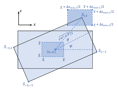
Figure 5: Illustration of $C(\underline{x},\underline{z},\underline{r},\bar{x},\bar{z},\bar{r},w,l)$ on $x-z$ plane.

As shown in fig. 5, we calculate the possible range for each of the four vertices of bounding box $S_{i}$. For example, fig. 5 illustrates that the $x-z$ coordinate of the upper-right vertex is $s_{1,1}=(x_{i}+\frac{\sqrt{w^{2}+l^{2}}}{2}\cos(\theta+\varphi),z_{i}+\frac{\sqrt{w^{2}+l^{2}}}{2}\sin(\theta+\varphi))$. Therefore, its $x,z$ coordinate of $s_{1,1}$satisfies

$$\underline{x}+\min_{\theta\in[\underline{r},\bar{r}]}\frac{1}{2}\sqrt{w^{2}+l^{2}}\cos(\theta+\varphi)\leq x_{1,1}\leq\bar{x}+\max_{\theta\in[\underline{r},\bar{r}]}\frac{1}{2}\sqrt{w^{2}+l^{2}}\cos(\theta+\varphi)$$ (53)

$$\underline{z}+\min_{\theta\in[\underline{r},\bar{r}]}\frac{1}{2}\sqrt{w^{2}+l^{2}}\sin(\theta+\varphi)\leq z_{1,1}\leq\bar{z}+\max_{\theta\in[\underline{r},\bar{r}]}\frac{1}{2}\sqrt{w^{2}+l^{2}}\sin(\theta+\varphi).$$ (54)

which means $s_{1,1}=(x_{1,1},z_{1,1})$ is contained by the rectangle formed by the four points in $S_{1,1}$, i.e., $s_{1,1}\in\mathrm{Conv}(P_{1,1})$. Similar arguments also hold for rest of vertices: $s_{1,-1}\in\mathrm{Conv}(P_{1,-1})$, $s_{-1,1}\in\mathrm{Conv}(P_{-1,1})$, and $s_{-1,-1}\in\mathrm{Conv}(P_{-1,-1})$. Finally, we conclude that

$$S_{i}=\mathrm{Conv}(s_{1,1},s_{1,-1},s_{-1,1},s_{-1,-1})\subseteq\mathrm{Conv}(P_{1,1},P_{1,-1},P_{-1,1},P_{-1,-1})$$ (55)

Note that $\underline{S}=C(\underline{x},\underline{z},\underline{r},\bar{x},\bar{z},\bar{r},\underline{w},\underline{l})$, and $\bar{S}=C(\underline{x},\underline{z},\underline{r},\bar{x},\bar{z},\bar{r},\bar{w},\bar{l})$. By eqs. 52 and 55,

$$\min_{x,z,r}\mathrm{Vol}(S_{i}(x,z,\underline{w},\underline{l},r)\cap S_{gt})\geq\underline{w}\underline{l}-\mathrm{Vol}(\underline{S}\backslash S_{gt})$$ (56)

and

$$\min_{x,z,r}\mathrm{Vol}(S_{i}(x,z,\bar{w},\bar{l},r)\cap S_{gt})\geq\bar{w}\bar{l}-\mathrm{Vol}(\bar{S}\backslash S_{gt}).$$ (57)

Combining the above, we have

$$\mathrm{IoU}(B_{i},B_{gt})\geq\frac{h_{1}(\underline{w}\underline{l}-\mathrm{Vol}(\underline{S}\backslash S_{gt}))}{hwl+\bar{h}\bar{w}\bar{l}-h_{2}(\bar{w}\bar{l}-\mathrm{Vol}(\bar{S}\backslash S_{gt}))}.$$ (58)

∎

Appendix C Additional Details of Certification Strategies

In this section, we present the details of our detection (Section C.1) and IoU (Section C.2) certification algorithms for camera and LiDAR fusion models, including the pseudocode and some details of our implementation. Note that our algorithms can be adapted to any fusion framework and single-modality model by doing smoothing inference and certification for corresponding modules.

C.1 Detection Certification

Algorithm 1 presents the pseudocode of our detection certification (function Certify) and median smoothing detection (function Inference). In our implementation, we directly sample on the left endpoints of each interval and do smoothing inference, which can also be replaced by a random point in each small interval.

Input: clean image input ${\bm{x}}_{0}\in{\mathcal{X}}\subseteq{\mathbb{R}}^{d}$, clean point cloud input ${\bm{p}}_{0}\in{\mathcal{P}}\subseteq{\mathbb{R}}^{3\times N}$, multi-sensor fusion pipeline $F:{\mathcal{X}}\times{\mathcal{P}}\to([C]\times[0,1])_{n}$, ground truth label $y$, image Gaussian noise variance $\sigma_{x}^{2}$, point Gaussian noise variance $\sigma_{p}^{2}$, transformation space $[{\bm{z}}_{l},{\bm{z}}_{u}]$, transformation function $T$, detection threshold $\gamma_{0}$

Output: smoothed confidence score of ground truth label $c_{median}$, lower bound and upper bound of confidence score of ground truth $c_{u},c_{l}$, whether the object is robustly detected as a boolean variable $b$

1 function Inference($F,{\bm{x}}_{0},{\bm{p}}_{0},y_{k},\sigma_{x},\sigma_{p},n,\gamma_{0}$):

2       $\hat{x}\leftarrow$ AddGaussianNoise $({\bm{x}}_{0},\sigma_{x},n)$

3       $\hat{p}\leftarrow$ AddGaussianNoise $({\bm{p}}_{0},\sigma_{p},n)$

4       $\hat{c}\leftarrow$ ComputeConfidenceScores $(F,\hat{x},\hat{p},y_{k})$

5       $\hat{c}\leftarrow$ Sort $(\hat{c})$

6       $c_{median}\leftarrow\hat{c}_{\lfloor 0.5n\rfloor}$

7       $b\leftarrow{\mathbb{I}}[c_{median}\geq\gamma_{0}]$

8       return $c_{median},b$

9 function Certify($F,{\bm{x}}_{0},{\bm{p}}_{0},y_{k},\sigma_{x},\sigma_{p},n,[{\bm{z}}_{l},{\bm{z}}_{u}],c,\alpha,\gamma_{0}$):

10       $interval\_list\leftarrow$ SplitInterval ($[{\bm{z}}_{l},{\bm{z}}_{u}]$)

11       $c_{median}\_list$, $c_{u}\_list$, $c_{l}\_list\leftarrow$ [], [], []

12       for $[z_{sl},z_{su}]\in$ interval_list do

             $\epsilon\leftarrow$ ComputeEps ($T,{\bm{x}}_{0},{\bm{p}}_{0},\sigma_{x},\sigma_{p},{\bm{z}}_{sl},{\bm{z}}_{su}$)

              $\triangleright$ compute ${\epsilon}$ according to equation (13)

13            

             $q_{u},q_{l}\leftarrow$ GetEmpiricalPerc $(n,\epsilon,c,\alpha/|\text{interval\_list}|)$

              $\triangleright$ compute $q_{u},q_{l}$ according to equation (10)

14            

15             $\hat{x}\leftarrow$ AddGaussianNoise $(T_{x}({\bm{x}}_{0},{\bm{z}}_{sl}),\sigma_{x},n)$

            

              $\triangleright$ sample $n$ Gaussian noises $\mathbf{\delta}_{x}\sim{\mathcal{N}}(0,\sigma_{x}^{2}{\bm{I}}_{d})$ and add to $T_{x}({\bm{x}}_{0},{\bm{z}}_{sl})$ to get $n$ noisy samples $\hat{x}$

16            

17             $\hat{p}\leftarrow$ AddGaussianNoise $(T_{p}({\bm{p}}_{0},{\bm{z}}_{sl}),\sigma_{p},n)$

            

              $\triangleright$ sample $n$ Gaussian noises $\mathbf{\delta}_{p}\sim{\mathcal{N}}(0,\sigma_{p}^{2}{\bm{I}}_{3\times N})$ and add to $(T_{p}({\bm{p}}_{0},{\bm{z}}_{sl})$ to get $n$ noisy samples $\hat{p}$

18            

19             $\hat{c}\leftarrow$ ComputeConfidenceScores $(F,\hat{x},\hat{p},y)$

            

              $\triangleright$ collect the confidence score of $y$ for each $({\bm{x}},{\bm{p}})\in(\hat{x},\hat{p})$ based on $F({\bm{x}},{\bm{p}})=\max_{1\leq k\leq\ell:y_{k}=y}c_{k}$

20            

21             $\hat{c}\leftarrow$ Sort $(\hat{c})$

22             $c_{median}\leftarrow\hat{c}_{\lfloor 0.5n\rfloor}$

23             if $q_{l}=-1$ then

                   $c_{l}\leftarrow-\infty$

                    $\triangleright$ $-\infty$ means cannot certify

24                  

25            else

26                   $c_{l}\leftarrow\hat{c}_{q_{l}}$

27            if $q_{u}=\infty$ then

                   $c_{u}\leftarrow\infty$

                    $\triangleright$ $\infty$ means cannot certify

28                  

29            else

30                   $c_{u}\leftarrow\hat{c}_{q_{u}}$

31            $c_{median}\_list$ add $c_{median}$, $c_{u}\_list$ add $c_{u}$, $c_{l}\_list$ add $c_{l}$

32      $b\leftarrow{\mathbb{I}}[\min c_{l}\_list\geq\gamma_{0}]$

33       return $\min c_{l}\_list$, $\max c_{u}\_list$, $b$

34      

35 function GetEmpiricalPerc $(n,\epsilon,c,\alpha)$:

36       $\underline{p}\leftarrow\Phi\left(\Phi^{-1}(p)-\epsilon\right)$

       $q_{l}\leftarrow\textnormal{{{BinarySearchLeft}}}(BinomialCDF(n,\underline{p}),1-\alpha)$

        $\triangleright$ do binary search and choose the left endpoint

37      

38       if $\text{BinomialCDF}(q_{l},\underline{p})>1-\alpha$ then

39             $q_{l}\leftarrow-1$

40      $\overline{p}\leftarrow\Phi\left(\Phi^{-1}(p)+\epsilon\right)$

       $q_{u}\leftarrow\textnormal{{{BinarySearchRight}}}(BinomialCDF(n,\overline{p}),\alpha)$

        $\triangleright$ do binary search and choose the right endpoint

41      

42       if $\text{BinomialCDF}(q_{u},\overline{p})<\alpha$ then

43             $q_{u}\leftarrow\infty$

44      return $q_{u},q_{l}$

Algorithm 1 0/1 Detection and Certification

C.2 IoU Certification

Algorithm 2 presents the pseudocode of our IoU certification (function Certify) and smoothing bounding box detection (function Inference). As in the detection certification framework, we also do sampling on the lower endpoint of each small interval. Algorithm 3 presents the pseudocode of IoU lower bound computation given the bounding box parameter intervals and the ground truth bounding box, and Algorithm 4 presents the pseudocode for computing the $x,z$ coordinate intervals for bounding box endpoints. Note that our framework focuses on the 7-parameter representation of bounding boxes ($x,y,z$, height, width, length, rotation angle), which can be adapted to other representation formats easily (e.g. 8 parameter representation, endpoint representation).

Input: clean image input ${\bm{x}}_{0}\in{\mathcal{X}}\subseteq{\mathbb{R}}^{d}$, clean point cloud input ${\bm{p}}_{0}\in{\mathcal{P}}\subseteq{\mathbb{R}}^{3\times N}$, multi-sensor fusion pipeline $F:{\mathcal{X}}\times{\mathcal{P}}\to([X]\times[Y]\times[Z]\times[W]\times[H]\times[L]\times[R]\times[C]\times[0,1])_{n}$, image Gaussian noise $\mathbf{\delta}_{x}\sim{\mathcal{N}}(0,\sigma_{x}^{2}{\bm{I}}_{d})$, point Gaussian noise $\mathbf{\delta}_{p}\sim{\mathcal{N}}(0,\sigma_{p}^{2}{\bm{I}}_{3\times N})$, transformation space $[{\bm{z}}_{l},{\bm{z}}_{u}]$.

Output: smoothed prediction $bbox_{median}$, lower bound of IoU between predicted bounding boxes and ground truth bounding boxes $\underline{IoU}$

1 function Inference($F,{\bm{x}}_{0},{\bm{p}}_{0},\sigma_{x},\sigma_{p},n$):

2       $\hat{x}\leftarrow$ AddGaussianNoise $({\bm{x}}_{0},\sigma_{x},n)$

3       $\hat{p}\leftarrow$ AddGaussianNoise $({\bm{p}}_{0},\sigma_{p},n)$

4       $\hat{bbox}\leftarrow$ ComputeBBoxParams ($F(\hat{x},\hat{p}))$

       $\hat{bbox}\leftarrow$ Sort $(\hat{bbox})$

        $\triangleright$ sort on each parameter

5      

       $bbox_{median}\leftarrow\hat{bbox}_{\lfloor 0.5n\rfloor}$

        $\triangleright$ take the median of each parameter

6      

7       return $bbox_{median}$

8 function Certify($F,{\bm{x}}_{0},{\bm{p}}_{0},\sigma_{x},\sigma_{p},n,[{\bm{z}}_{sl},{\bm{z}}_{su}],c,\alpha$):

9       $interval\_list\leftarrow$ SplitInterval ($[{\bm{z}}_{sl},{\bm{z}}_{su}]$)

10       $IoU\_list\leftarrow$ []

11       for $[z_{sl},z_{su}]\in$ interval_list do

             $\epsilon\leftarrow$ ComputeEps ($T,{\bm{x}}_{0},{\bm{p}}_{0},\sigma_{x},\sigma_{p},{\bm{z}}_{l},{\bm{z}}_{u}$)

              $\triangleright$ compute ${\epsilon}$ according to equation (13)

12            

             $q_{u},q_{l}\leftarrow$ GetEmpiricalPerc $(n,\epsilon,c,\alpha/|\text{interval\_list}|)$

              $\triangleright$ compute $q_{u},q_{l}$ according to equation (10)

13            

14             $\hat{x}\leftarrow$ AddGaussianNoise $(T_{x}({\bm{x}}_{0},{\bm{z}}_{sl}),\sigma_{x},n)$

            

              $\triangleright$ sample $n$ Gaussian noises $\mathbf{\delta}_{x}\sim{\mathcal{N}}(0,\sigma_{x}^{2}{\bm{I}}_{d})$ and add to $T_{x}({\bm{x}}_{0},{\bm{z}}_{sl})$ to get $n$ noisy samples $\hat{x}$

15            

16             $\hat{p}\leftarrow$ AddGaussianNoise $(T_{p}({\bm{p}}_{0},{\bm{z}}_{sl}),\sigma_{p},n)$

            

              $\triangleright$ sample $n$ Gaussian noises $\mathbf{\delta}_{p}\sim{\mathcal{N}}(0,\sigma_{p}^{2}{\bm{I}}_{3\times N})$ and add to $(T_{p}({\bm{p}}_{0},{\bm{z}}_{sl})$ to get $n$ noisy samples $\hat{p}$

17            

18             $\hat{bbox}\leftarrow$ ComputeBBoxParams ($F(\hat{x},\hat{p}))$

             $\hat{bbox}\leftarrow$ Sort $(\hat{bbox})$

              $\triangleright$ sort on each parameter

19            

20             if $q_{l}=-1$ then

                   $\underline{IoU}\leftarrow-\infty$

                    $\triangleright$ $-\infty$ means cannot certify

21                  

22                   return $\underline{IoU}$

23            else

24                   $bbox_{l}\leftarrow\hat{bbox}_{q_{l}}$

25            if $q_{u}=\infty$ then

                   $\underline{IoU}\leftarrow\infty$

                    $\triangleright$ $\infty$ means cannot certify

26                  

27                   return $\underline{IoU}$

28            else

29                   $bbox_{u}\leftarrow\hat{bbox}_{q_{u}}$

30            $\underline{IoU}\leftarrow$ IoULowerBound ($\underline{bbox},\overline{bbox},bbox$)

31             $IoU\_list$ add $\underline{IoU}$

32      return $\min(IoU\_list)$

33function GetEmpiricalPerc $(n,\epsilon,c,\alpha)$:

34       $\underline{p}\leftarrow\Phi\left(\Phi^{-1}(p)-\epsilon\right)$

       $q_{l}\leftarrow\textnormal{{{BinarySearchLeft}}}(BinomialCDF(n,\underline{p}),1-\alpha)$

        $\triangleright$ do binary search and choose the left endpoint

35      

36       if $\text{BinomialCDF}(q_{l},\underline{p})>1-\alpha$ then

37             $q_{l}\leftarrow-1$

38      $\overline{p}\leftarrow\Phi\left(\Phi^{-1}(p)+\epsilon\right)$

       $q_{u}\leftarrow\textnormal{{{BinarySearchRight}}}(BinomialCDF(n,\overline{p}),\alpha)$

        $\triangleright$ do binary search and choose the right endpoint

39      

40       if $\text{BinomialCDF}(q_{u},\overline{p})<\alpha$ then

41             $q_{u}\leftarrow\infty$

42      return $q_{u},q_{l}$

Algorithm 2 Bounding Box Detection and Certification

Input: upper bound of bounding boxes’ parameters $\overline{bbox}$, lower bound of bounding boxes’ parameters $\underline{bbox}$, ground truth bounding boxes’ parameters $bbox$

Output: lower bound of IoU between predicted bounding boxes and ground truth bounding boxes $\underline{IoU}$

1 function IoULowerBound($\overline{bbox},\underline{bbox},bbox$):

2       $\underline{V_{I}}\leftarrow$ IntersectionLowerBound ($\overline{bbox},\underline{bbox},bbox$)

3       $\overline{V_{U}}\leftarrow$ UnionUpperBound ($\overline{bbox},\underline{bbox},bbox$)

4       return $\underline{V_{I}}/\overline{V_{U}}$

5function IntersectionLowerBound $(\overline{bbox},\underline{bbox},bbox)$:

6       if $y<(\overline{y}+\underline{y})/2$ then

7             $y_{l}=\overline{y}$

8      else

9             $y_{l}=\underline{y}$

10      if $y\leq y_{l}-\underline{h}$ $\mathbf{or}$ $y_{l}\leq y-h$ then

11             return $0$

12      else

13             $h_{I}=\min(y_{l},y)-\max(y_{l}-\underline{h},y-h)$

14      $xz_{l},xz_{u}\leftarrow$ CornerXZIntervals ($\underline{l},\underline{w},\underline{x},\underline{z},\underline{r},\overline{x},\overline{z},\overline{r}$)

15       $\underline{S_{overlap}}\leftarrow$ OverlapAreaLower ($xz_{l},xz_{u},bbox$)

16       if $\underline{S_{overlap}}\leq 0$ then

17             return $0$

18      else

19             return $h_{I}\cdot\underline{S_{overlap}}$

20      

21function UnionUpperBound $(\overline{bbox},\underline{bbox},bbox)$:

22       if $y<(\overline{y}+\underline{y})/2$ then

23             $y_{u}=\underline{y}$

24      else

25             $y_{u}=\overline{y}$

26      if $y\leq y_{u}-\overline{h}$ $\mathbf{or}$ $y_{u}\leq y-h$ then

27             return $0$

28      else

29             $h_{I}=\min(y_{u},y)-\max(y_{u}-\overline{h},y-h)$

30      $xz_{l},xz_{u}\leftarrow$ CornerXZIntervals ($\overline{l},\overline{w},\underline{x},\underline{z},\underline{r},\overline{x},\overline{z},\overline{r}$)

31       $\underline{S_{overlap}}\leftarrow$ OverlapAreaLower ($xz_{l},xz_{u},bbox$)

32       if $\underline{S_{overlap}}\leq 0$ then

33             return $h\cdot w\cdot l+\overline{h}\cdot\overline{w}\cdot\overline{l}$

34      else

35             return $h\cdot w\cdot l+\overline{h}\cdot\overline{w}\cdot\overline{l}-h_{I}\cdot\underline{S_{overlap}}$

36      

Algorithm 3 IoU Lower Bound

Input: bounding box length $l$, width $w$, $x$ lower bound $\underline{x}$, $z$ lower bound $\underline{z}$, rotation angel lower bound $\underline{r}$, $x$ upper bound $\overline{x}$, $z$ upper bound $\overline{z}$, rotation upper bound $\overline{r}$

Output: bounding box corners’ $xz$ coordinates lower bound $xz_{l}$, bounding box corners’ xz coordinates upper bound $xz_{u}$

1 function CornerXZIntervals ($l,w,\underline{x},\underline{z},\underline{r},\overline{x},\overline{z},\overline{r}$):

2       $xzCoorsList\leftarrow\left[\right]$

3       for $x,z$ $\mathbf{in}$ $\left[\left[\underline{x},\underline{z}\right],\left[\overline{x},\overline{z}\right]\right]$  do

4             for $r$ $\mathbf{in}$ $\underline{r},\overline{r}$ do

5                   $xzCoors\leftarrow$ ComputeXZ ($x,z,r$)

6                   $xzCoorsList$ add $xzCoors$

7            

      $xz_{l},xz_{u}\leftarrow$ ComputeXZInterval ($xzCoorsList$)

        $\triangleright$ compute $x,z$ intervals roughly

8      

      

       $\triangleright$ consider extremum cases

9       $\alpha\leftarrow\arctan(w/l)$

10       $d\leftarrow\sqrt{\left(l/2\right)^{2}+\left(w/2\right)^{2}}$

11       if $\pi-\alpha\geq\underline{r}$ $\mathbf{and}$ $\pi-\alpha\leq\overline{r}$ then

12             $xz_{l}[0]\leftarrow\underline{x}-d$

13             $xz_{u}[4]\leftarrow\overline{x}+d$

14      if $2\pi-\alpha\geq\underline{r}$ $\mathbf{and}$ $2\pi-\alpha\leq\overline{r}$ then

15             $xz_{u}[0]\leftarrow\overline{x}+d$

16             $xz_{l}[4]\leftarrow\underline{x}-d$

17      if $\pi/2-\alpha\geq\underline{r}$ $\mathbf{and}$ $\pi/2-\alpha\leq\overline{r}$ then

18             $xz_{u}[1]\leftarrow\overline{z}+d$

19             $xz_{l}[5]\leftarrow\underline{z}-d$

20      if $3\pi/2-\alpha\geq\underline{r}$ $\mathbf{and}$ $3\pi/2-\alpha\leq\overline{r}$ then

21             $xz_{l}[1]\leftarrow\underline{z}-d$

22             $xz_{u}[5]\leftarrow\overline{z}+d$

23      if $\alpha\geq\underline{r}$ $\mathbf{and}$ $\alpha\leq\overline{r}$ then

24             $xz_{u}[2]\leftarrow\overline{x}+d$

25             $xz_{l}[6]\leftarrow\underline{x}-d$

26      if $\pi+\alpha\geq\underline{r}$ $\mathbf{and}$ $\pi+\alpha\leq\overline{r}$ then

27             $xz_{l}[2]\leftarrow\underline{x}-d$

28             $xz_{u}[6]\leftarrow\overline{x}+d$

29      if $\pi/2+\alpha\geq\underline{r}$ $\mathbf{and}$ $\pi/2+\alpha\leq\overline{r}$ then

30             $xz_{u}[3]\leftarrow\overline{z}+d$

31             $xz_{l}[7]\leftarrow\underline{z}-d$

32      if $3\pi/2+\alpha\geq\underline{r}$ $\mathbf{and}$ $3\pi/2+\alpha\leq\overline{r}$ then

33             $xz_{l}[3]\leftarrow\underline{z}-d$

34             $xz_{u}[7]\leftarrow\overline{z}+d$

35      

return $xz_{l},xz_{u}$

Algorithm 4 Corners’ $x,z$ Intervals

Appendix D Additional Experimental Details

D.1 Dataset

Table 3: Certification data. Each row stands for one setting, and the columns “vehicle color", “building", “pedestrian", and “amount" represent the color of the car, whether buildings exist, whether a pedestrian exists, and the number of corresponding data respectively.

vehicle color	building	pedestrian	amount
blue	yes	no	15
red	yes	no	4
red	yes	yes	4
black	yes	no	4
black	yes	yes	4
blue	no	no	15
red	no	no	4
red	no	yes	4
black	no	no	4
black	no	yes	4

As introduced in Section 4, we generate the certification data via spawning the ego vehicle at a few randomly chosen spawn points. For settings with 15 spawn points in Table 3, the randomly-chosen spawn point index in the CARLA Town01 map is 15, 30, 43, 46, 57, 86, 102, 11, 136, 14, 29, 6, 61, 81, and 88. For settings with 4 spawn points in Table 3, the randomly-chosen spawn point index is 15, 30, 43, and 46.

Certification setup.

As reflected in Lemma 3.3, to certify the robustness, we need to partition the transformation’s parameter space. For rotation certification, we split the rotation angle interval $[-30^{\circ},30^{\circ}]$ uniformly into 600 tiny intervals of 0.1 degree; for shifting certification, we split the distance interval $[10,15]$ uniformly into 500 tiny intervals of 0.01 meter.

Empirical attack setup.

In Section 4, we evaluate the empirical robustness, i.e., the robustness under attacks, to show vanilla models’ vulnerability and estimate the certification tightness. For rotation, we conduct the attack by enumerating the lowest detection rate and IoU score among 6000 parameters uniformly sampled with a distance 0.01 degree (distance = $60^{\circ}/6000=0.01^{\circ}$); for shifting, we conduct the attack by enumerating the lowest detection rate and IoU score among 5000 parameters uniformly sampled with a distance of 0.001 meter (distance = $5/5000=0.001$).

D.2 Detailed Experimental Evaluation

In this section, we present the complete experimental results, which include rotation transformation (Table 4(b)) and shifting transformation (Table 5(b)) considering different thresholds for detection and IoU certification.

Certification against rotation transformation.

As shown in Table 4(b) and discussed in Section 4.1, the order of robustness against rotation transformation in the detection metric is $\text{FocalsConv}>\text{MonoCon}>\text{CLOCs}>\text{SECOND}$, but the most robust model in the IoU metric is CLOCs. Moreover, with experimental results in different thresholds (Table 4(b), Table 6(a) and Figure 3), the performance of models all drop when the threshold or attack radius increase, and all models’ certified IoU drop to 0 when $\text{TH}_{\text{IoU}}\approx 0.6$ , which reflects the problem of models’ robustness against rotation transformation. We can also find that the performance difference between models increases when the threshold or attack radius increases.

Certification against shifting transformation.

As shown in Table 5(b) and discussed in Section 4.2, the order of robustness against shifting transformation in the detection metric is $\text{CLOCs}>\text{SECOND}\approx\text{MonoCon}>\text{FocalsConv}$, and the order in the IoU metric is $\text{CLOCs}>\text{MonoCon}>\text{SECOND}>\text{FocalsConv}$. This shows the advantage of fusion models (e.g. CLOCs) on the one hand but also shows this makes the attack space larger on another hand (e.g. FocalsConv), which leads to a new question of robust fusion mechanism design.

Table 4: Overview of rotation transformation experiment results (smoothing $\sigma=0.25$). Each row represents the corresponding model and attack radius. “Benign”, “Adv (Vanilla)”, “Adv (Smoothed)”, and “Certification” stands for benign performance, vanilla models’ performance under attacks, smoothed models’ performance under attacks, and certified lower bound of smoothed model performance under attacks. Each column represents the results under different thresholds.

(a) Detection rate under rotation transformation

Model	Attack Radius	Benign			Adv (Vanilla)			Adv (Smoothed)			Certification
		Det@20	Det@50	Det@80	Det@20	Det@50	Det@80	Det@20	Det@50	Det@80	Det@20	Det@50	Det@80
MonoCon [30]	$|r|\leq 10^{\circ}$	100.00%	100.00%	100.00%	70.97%	70.97%	58.06%	98.39%	98.39%	80.65%	95.16%	95.16%	75.81%
	$|r|\leq 15^{\circ}$				70.97%	70.97%	58.06%	98.39%	98.39%	80.65%	95.16%	95.16%	75.81%
	$|r|\leq 20^{\circ}$				70.97%	70.97%	58.06%	98.39%	98.39%	80.65%	95.16%	95.16%	75.81%
	$|r|\leq 25^{\circ}$				70.97%	70.97%	45.16%	98.39%	98.39%	80.65%	95.16%	95.16%	75.81%
	$|r|\leq 30^{\circ}$				70.97%	70.97%	32.26%	96.77%	96.77%	80.65%	91.94%	91.94%	75.81%
SECOND [50]	$|r|\leq 10^{\circ}$	100.00%	100.00%	100.00%	100.00%	100.00%	0.00%	100.00%	100.00%	0.00%	100.00%	100.00%	0.00%
	$|r|\leq 15^{\circ}$				100.00%	100.00%	0.00%	100.00%	100.00%	0.00%	100.00%	100.00%	0.00%
	$|r|\leq 20^{\circ}$				100.00%	100.00%	0.00%	100.00%	100.00%	0.00%	100.00%	100.00%	0.00%
	$|r|\leq 25^{\circ}$				100.00%	12.90%	0.00%	100.00%	100.00%	0.00%	100.00%	100.00%	0.00%
	$|r|\leq 30^{\circ}$				67.74%	3.23%	0.00%	100.00%	100.00%	0.00%	100.00%	62.90%	0.00%
CLOCs [34]	$|r|\leq 10^{\circ}$	100.00%	100.00%	100.00%	100.00%	100.00%	100.00%	100.00%	100.00%	88.71%	100.00%	100.00%	88.71%
	$|r|\leq 15^{\circ}$				100.00%	100.00%	100.00%	98.39%	79.03%	66.13%	98.39%	77.42%	66.13%
	$|r|\leq 20^{\circ}$				100.00%	100.00%	100.00%	98.39%	69.35%	50.00%	98.39%	67.74%	50.00%
	$|r|\leq 25^{\circ}$				100.00%	91.94%	20.97%	98.39%	69.35%	50.00%	98.39%	67.74%	50.00%
	$|r|\leq 30^{\circ}$				100.00%	74.19%	3.23%	98.39%	69.35%	50.00%	98.39%	67.74%	50.00%
FocalsConv [6]	$|r|\leq 10^{\circ}$	100.00%	100.00%	100.00%	100.00%	100.00%	100.00%	100.00%	100.00%	100.00%	100.00%	100.00%	100.00%
	$|r|\leq 15^{\circ}$				100.00%	100.00%	100.00%	100.00%	100.00%	100.00%	100.00%	100.00%	100.00%
	$|r|\leq 20^{\circ}$				100.00%	100.00%	100.00%	100.00%	100.00%	100.00%	100.00%	100.00%	100.00%
	$|r|\leq 25^{\circ}$				100.00%	100.00%	100.00%	100.00%	100.00%	100.00%	100.00%	100.00%	100.00%
	$|r|\leq 30^{\circ}$				100.00%	100.00%	98.39%	100.00%	100.00%	100.00%	100.00%	100.00%	100.00%

(b) IoU with ground truth under rotation transformation

Model	Attack Radius	Benign			Adv (Vanilla)			Adv (Smoothed)			Certification
		AP@30	AP@50	AP@80	AP@30	AP@50	AP@80	AP@30	AP@50	AP@80	AP@30	AP@50	AP@80
MonoCon [30]	$|r|\leq 10^{\circ}$	100.00%	100.00%	100.00%	56.45%	56.45%	0.00%	82.26%	82.26%	0.00%	75.81%	0.00%	0.00%
	$|r|\leq 15^{\circ}$				54.84%	54.84%	0.00%	82.26%	82.26%	0.00%	74.19%	0.00%	0.00%
	$|r|\leq 20^{\circ}$				54.84%	53.23%	0.00%	82.26%	74.19%	0.00%	6.45%	0.00%	0.00%
	$|r|\leq 25^{\circ}$				51.61%	16.13%	0.00%	80.65%	16.13%	0.00%	0.00%	0.00%	0.00%
	$|r|\leq 30^{\circ}$				46.77%	0.00%	0.00%	79.03%	3.23%	0.00%	0.00%	0.00%	0.00%
SECOND [50]	$|r|\leq 10^{\circ}$	100.00%	100.00%	100.00%	96.77%	96.77%	0.00%	100.00%	100.00%	100.00%	100.00%	100.00%	0.00%
	$|r|\leq 15^{\circ}$				96.77%	96.77%	0.00%	100.00%	100.00%	100.00%	100.00%	100.00%	0.00%
	$|r|\leq 20^{\circ}$				96.77%	96.77%	0.00%	100.00%	100.00%	54.84%	100.00%	100.00%	0.00%
	$|r|\leq 25^{\circ}$				83.87%	83.87%	0.00%	100.00%	96.77%	0.00%	100.00%	0.00%	0.00%
	$|r|\leq 30^{\circ}$				51.61%	51.61%	0.00%	54.84%	54.84%	0.00%	11.29%	0.00%	0.00%
CLOCs [34]	$|r|\leq 10^{\circ}$	100.00%	100.00%	100.00%	90.32%	90.32%	90.32%	100.00%	100.00%	98.39%	100.00%	100.00%	0.00%
	$|r|\leq 15^{\circ}$				90.32%	90.32%	90.32%	98.39%	98.39%	85.48%	98.39%	87.10%	0.00%
	$|r|\leq 20^{\circ}$				88.71%	88.71%	77.42%	98.39%	98.39%	67.74%	98.39%	69.35%	0.00%
	$|r|\leq 25^{\circ}$				87.10%	87.10%	0.00%	98.39%	98.39%	67.74%	98.39%	67.74%	0.00%
	$|r|\leq 30^{\circ}$				80.65%	80.65%	0.00%	98.39%	98.39%	67.74%	98.39%	53.23%	0.00%
FocalsConv [6]	$|r|\leq 10^{\circ}$	100.00%	100.00%	100.00%	96.77%	96.77%	0.00%	100.00%	100.00%	0.00%	100.00%	0.00%	0.00%
	$|r|\leq 15^{\circ}$				96.77%	0.00%	0.00%	100.00%	0.00%	0.00%	0.00%	0.00%	0.00%
	$|r|\leq 20^{\circ}$				96.77%	0.00%	0.00%	100.00%	0.00%	0.00%	0.00%	0.00%	0.00%
	$|r|\leq 25^{\circ}$				96.77%	0.00%	0.00%	100.00%	0.00%	0.00%	0.00%	0.00%	0.00%
	$|r|\leq 30^{\circ}$				96.77%	0.00%	0.00%	100.00%	0.00%	0.00%	0.00%	0.00%	0.00%

Table 5: Overview of shifting transformation experiment results. Each row represents the corresponding model and attack radius. “Benign”, “Adv (Vanilla)”, “Adv (Smoothed)”, and “Certification” stands for benign performance, vanilla models’ performance under attacks, smoothed models’ performance under attacks, and certified lower bound of smoothed model performance under attacks. Each column represents the results under different thresholds.

(a) Detection rate under shifting transformation

Model	Attack Radius	Benign			Adv (Vanilla)			Adv (Smoothed)			Certification
		Det@20	Det@50	Det@80	Det@20	Det@50	Det@80	Det@20	Det@50	Det@80	Det@20	Det@50	Det@80
MonoCon [30]	$10\leq z\leq 11$	100.00%	100.00%	100.00%	87.10%	87.10%	66.13%	87.10%	87.10%	66.13%	83.87%	83.87%	64.52%
	$10\leq z\leq 12$				85.48%	85.48%	62.90%	85.48%	85.48%	62.90%	75.81%	75.81%	61.29%
	$10\leq z\leq 13$				82.26%	82.26%	56.45%	82.26%	82.26%	56.45%	72.58%	72.58%	51.61%
	$10\leq z\leq 14$				75.81%	75.81%	46.77%	75.81%	75.81%	46.77%	66.13%	66.13%	41.94%
	$10\leq z\leq 15$				50.00%	50.00%	27.42%	50.00%	50.00%	27.42%	48.39%	48.39%	27.42%
SECOND [50]	$10\leq z\leq 11$	100.00%	100.00%	100.00%	100.00%	70.97%	0.00%	100.00%	70.97%	0.00%	100.00%	0.00%	0.00%
	$10\leq z\leq 12$				100.00%	70.97%	0.00%	100.00%	70.97%	0.00%	100.00%	0.00%	0.00%
	$10\leq z\leq 13$				100.00%	12.90%	0.00%	100.00%	70.97%	0.00%	100.00%	0.00%	0.00%
	$10\leq z\leq 14$				100.00%	12.90%	0.00%	100.00%	70.97%	0.00%	100.00%	0.00%	0.00%
	$10\leq z\leq 15$				100.00%	12.90%	0.00%	100.00%	70.97%	0.00%	100.00%	0.00%	0.00%
CLOCs [34]	$10\leq z\leq 11$	100.00%	100.00%	100.00%	100.00%	100.00%	93.54%	100.00%	100.00%	93.54%	100.00%	100.00%	67.74%
	$10\leq z\leq 12$				100.00%	100.00%	93.54%	100.00%	100.00%	93.54%	100.00%	100.00%	66.13%
	$10\leq z\leq 13$				100.00%	100.00%	85.45%	100.00%	100.00%	88.71%	100.00%	100.00%	64.52%
	$10\leq z\leq 14$				100.00%	100.00%	64.52%	100.00%	100.00%	85.48%	100.00%	100.00%	62.90%
	$10\leq z\leq 15$				100.00%	100.00%	64.52%	100.00%	100.00%	83.87%	100.00%	100.00%	61.29%
FocalsConv [6]	$10\leq z\leq 11$	100.00%	100.00%	100.00%	100.00%	100.00%	96.77%	100.00%	100.00%	96.77%	91.94%	88.71%	54.84%
	$10\leq z\leq 12$				100.00%	100.00%	96.77%	100.00%	100.00%	96.77%	87.10%	79.03%	4.84%
	$10\leq z\leq 13$				82.26%	22.58%	0.00%	82.26%	22.58%	0.00%	4.84%	0.00%	0.00%
	$10\leq z\leq 14$				14.52%	0.00%	0.00%	14.52%	0.00%	0.00%	0.00%	0.00%	0.00%
	$10\leq z\leq 15$				8.06%	0.00%	0.00%	8.06%	0.00%	0.00%	0.00%	0.00%	0.00%

(b) IoU with ground truth under shifting transformation

Model	Attack Radius	Benign			Adv (Vanilla)			Adv (Smoothed)			Certification
		AP@30	AP@50	AP@80	AP@30	AP@50	AP@80	AP@30	AP@50	AP@80	AP@30	AP@50	AP@80
MonoCon [30]	$10\leq z\leq 11$	100.00%	100.00%	100.00%	77.42%	77.42%	41.94%	77.42%	77.42%	41.94%	74.19%	41.94%	0.00%
	$10\leq z\leq 12$				74.19%	74.19%	0.00%	74.19%	74.19%	0.00%	69.35%	1.61%	0.00%
	$10\leq z\leq 13$				72.58%	72.58%	0.00%	72.58%	72.58%	0.00%	61.29%	0.00%	0.00%
	$10\leq z\leq 14$				40.32%	33.87%	0.00%	40.32%	33.87%	0.00%	20.97%	0.00%	0.00%
	$10\leq z\leq 15$				6.45%	1.61%	0.00%	6.45%	1.61%	0.00%	0.00%	0.00%	0.00%
SECOND [50]	$10\leq z\leq 11$	100.00%	100.00%	100.00%	93.55%	93.55%	93.55%	100.00%	100.00%	0.00%	0.00%	0.00%	0.00%
	$10\leq z\leq 12$				93.55%	93.55%	93.55%	100.00%	100.00%	0.00%	0.00%	0.00%	0.00%
	$10\leq z\leq 13$				87.10%	87.10%	87.10%	100.00%	100.00%	0.00%	0.00%	0.00%	0.00%
	$10\leq z\leq 14$				87.10%	87.10%	87.10%	100.00%	100.00%	0.00%	0.00%	0.00%	0.00%
	$10\leq z\leq 15$				87.10%	87.10%	87.10%	100.00%	100.00%	0.00%	0.00%	0.00%	0.00%
CLOCs [34]	$10\leq z\leq 11$	100.00%	100.00%	100.00%	93.55%	93.55%	93.55%	100.00%	100.00%	100.00%	79.03%	79.03%	0.00%
	$10\leq z\leq 12$				80.65%	80.65%	80.65%	80.65%	80.65%	80.65%	51.61%	51.61%	0.00%
	$10\leq z\leq 13$				80.65%	80.65%	77.42%	80.65%	80.65%	77.42%	51.61%	48.39%	0.00%
	$10\leq z\leq 14$				80.65%	80.65%	77.42%	80.65%	80.65%	77.42%	51.61%	48.39%	0.00%
	$10\leq z\leq 15$				80.65%	80.65%	77.42%	80.65%	80.65%	77.42%	51.61%	48.39%	0.00%
FocalsConv [6]	$10\leq z\leq 11$	100.00%	100.00%	100.00%	97.77%	0.00%	0.00%	100.00%	100.00%	0.00%	85.48%	0.00%	0.00%
	$10\leq z\leq 12$				0.00%	0.00%	0.00%	100.00%	100.00%	0.00%	83.87%	0.00%	0.00%
	$10\leq z\leq 13$				0.00%	0.00%	0.00%	82.26%	82.26%	0.00%	4.84%	0.00%	0.00%
	$10\leq z\leq 14$				0.00%	0.00%	0.00%	14.52%	14.52%	0.00%	0.00%	0.00%	0.00%
	$10\leq z\leq 15$				0.00%	0.00%	0.00%	8.06%	8.06%	0.00%	0.00%	0.00%	0.00%

	$\text{TH}_{\text{conf}}=0.2$	$\text{TH}_{\text{conf}}=0.5$	$\text{TH}_{\text{conf}}=0.8$	$\text{TH}_{\text{IoU}}=0.3$	$\text{TH}_{\text{IoU}}=0.5$	$\text{TH}_{\text{IoU}}=0.8$
Detection			IoU
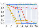
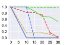
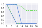
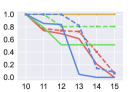
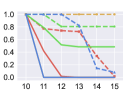
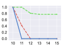
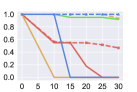
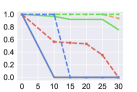
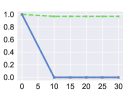
	attack $\epsilon$	attack $\epsilon$	attack $\epsilon$	attack $\epsilon$	attack $\epsilon$	attack $\epsilon$

(a) Robustness certification for rotation transformation (smoothing $\sigma=0.25$)

	$\text{TH}_{\text{conf}}=0.2$	$\text{TH}_{\text{conf}}=0.5$	$\text{TH}_{\text{conf}}=0.8$	$\text{TH}_{\text{IoU}}=0.3$	$\text{TH}_{\text{IoU}}=0.5$	$\text{TH}_{\text{IoU}}=0.8$
Detection			IoU
	attack $\epsilon$	attack $\epsilon$	attack $\epsilon$	attack $\epsilon$	attack $\epsilon$	attack $\epsilon$

(b) Robustness certification for shift transformation

	$\text{TH}_{\text{conf}}=0.2$	$\text{TH}_{\text{conf}}=0.5$	$\text{TH}_{\text{conf}}=0.8$	$\text{TH}_{\text{IoU}}=0.3$	$\text{TH}_{\text{IoU}}=0.5$	$\text{TH}_{\text{IoU}}=0.8$
Detection			IoU
	attack $\epsilon$	attack $\epsilon$	attack $\epsilon$	attack $\epsilon$	attack $\epsilon$	attack $\epsilon$

(c) Robustness certification for rotation transformation (smoothing $\sigma=0.5$)

Figure 6: Robustness certification for rotation and shifting transformation, including detection rate bound and IoU bound. Solid lines represent the certified bounds, and dashed lines show the empirical performance under PGD.

	$10\leq z\leq 11$	$10\leq z\leq 12$	$10\leq z\leq 13$	$10\leq z\leq 14$	$10\leq z\leq 15$
Detection
	$\text{TH}_{\text{conf}}$	$\text{TH}_{\text{conf}}$	$\text{TH}_{\text{conf}}$	$\text{TH}_{\text{conf}}$	$\text{TH}_{\text{conf}}$
IoU
	$\text{TH}_{\text{IoU}}$	$\text{TH}_{\text{IoU}}$	$\text{TH}_{\text{IoU}}$	$\text{TH}_{\text{IoU}}$	$\text{TH}_{\text{IoU}}$

Figure 7: Robustness certification for shifting transformation, including detection rate bound and IoU bound. Solid lines represent the certified bounds, and dashed lines show the empirical performance under PGD.

D.3 Effect of Sample Strategy

To study the effect of sampling strategies, we compare two different sampling strategies and show the results in Table 7(b). The first strategy is fixing the size of intervals (e.g. $0.1^{\circ}$ rotation intervals in out case), which is named “Certification (sparse)” in Table 7(b), and the second strategy is fixing small interval number (e.g. 600 small intervals in each big rotation interval), which is called “Certification (dense)" in Table 7(b).

From certified detection rate Table 7(a) and certified IoU Table 7(b), we can find that the “Certification (sparse)" is already tight enough when the sample number in each small interval stays the same since the certified detection rate and IoU in “Certification (sparse)" is almost the same as those in “Certification (dense)".

Table 7: Overview of rotation transition experiment results with different sampling strategies under the condition “color 1 with buildings without pedestrian”. Each row represents the corresponding model and attack radius. Columns “Certification (sparse)”, and “Certification (dense)” represent the certified lower bound of performance under attacks with intervals of $0.1^{\circ}$ and 600 intervals respectively.

(a) Certified rotation detection rate.

Model	Attack Radius	Certification (sparse)			Certification (dense)
		Det@20	Det@50	Det@80	Det@20	Det@50	Det@80
MonoCon [30]	$r\pm 10^{\circ}$	93.33%	93.33%	86.67%	93.33%	93.33%	86.67%
	$r\pm 20^{\circ}$	93.33%	93.33%	86.67%	93.33%	93.33%	86.67%
	$r\pm 30^{\circ}$	86.67%	86.67%	86.67%	86.67%	86.67%	86.67%
SECOND [50]	$r\pm 10^{\circ}$	100.00%	100.00%	0.00%	100.00%	100.00%	0.00%
	$r\pm 20^{\circ}$	100.00%	100.00%	0.00%	100.00%	100.00%	0.00%
	$r\pm 30^{\circ}$	100.00%	66.67%	0.00%	100.00%	66.67%	0.00%
CLOCs [34]	$r\pm 10^{\circ}$	100.00%	100.00%	100.00%	100.00%	100.00%	100.00%
	$r\pm 20^{\circ}$	100.00%	80.00%	73.33%	100.00%	80.00%	73.33%
	$r\pm 30^{\circ}$	100.00%	80.00%	73.33%	100.00%	80.00%	73.33%
FocalsConv [6]	$r\pm 10^{\circ}$	100.00%	100.00%	100.00%	100.00%	100.00%	100.00%
	$r\pm 20^{\circ}$	100.00%	100.00%	100.00%	100.00%	100.00%	100.00%
	$r\pm 30^{\circ}$	100.00%	100.00%	100.00%	100.00%	100.00%	100.00%

(b) Certified rotation IoU.

Model	Attack Radius	Certification (sparse)			Certification (dense)
		AP@30	AP@50	AP@70	AP@30	AP@50	AP@70
MonoCon [30]	$r\pm 10^{\circ}$	86.67%	0.00%	0.00%	86.67%	0.00%	0.00%
	$r\pm 20^{\circ}$	13.33%	0.00%	0.00%	13.33%	0.00%	0.00%
	$r\pm 30^{\circ}$	0.00%	0.00%	0.00%	0.00%	0.00%	0.00%
SECOND [50]	$r\pm 10^{\circ}$	0.00%	0.00%	0.00%	0.00%	0.00%	0.00%
	$r\pm 20^{\circ}$	0.00%	0.00%	0.00%	0.00%	0.00%	0.00%
	$r\pm 30^{\circ}$	0.00%	0.00%	0.00%	0.00%	0.00%	0.00%
CLOCs [34]	$r\pm 10^{\circ}$	100.00%	100.00%	0.00%	100.00%	100.00%	0.00%
	$r\pm 20^{\circ}$	100.00%	93.33%	0.00%	100.00%	93.33%	0.00%
	$r\pm 30^{\circ}$	100.00%	53.33%	0.00%	100.00%	53.33%	0.00%
FocalsConv [6]	$r\pm 10^{\circ}$	100.00%	0.00%	0.00%	100.00%	0.00%	0.00%
	$r\pm 20^{\circ}$	0.00%	0.00%	0.00%	13.33%	0.00%	0.00%
	$r\pm 30^{\circ}$	0.00%	0.00%	0.00%	0.00%	0.00%	0.00%

D.4 Effect of Smoothing Parameter $\sigma$

To study the effect of smoothing parameter $\sigma$, we test our approach with random Gaussian noise whose $\sigma=0.5$ in our rotation setting to compare the previous results on rotation transformation with noises whose $\sigma=0.25$ (Table 4(b)).

As shown in Table 6(c), Figure 8 and Table 8(b), the models’ performance might degrade in small attack radius with larger smoothing $\sigma$, but smoothing with larger $\sigma$ can also improve the robustness of models against large attack radius, especially for the model which is more stable than others (CLOCs in our case).

	$|r|\leq 10^{\circ}$	$|r|\leq 15^{\circ}$	$|r|\leq 20^{\circ}$	$|r|\leq 25^{\circ}$	$|r|\leq 30^{\circ}$
Detection
	$\text{TH}_{\text{conf}}$	$\text{TH}_{\text{conf}}$	$\text{TH}_{\text{conf}}$	$\text{TH}_{\text{conf}}$	$\text{TH}_{\text{conf}}$
IoU
	$\text{TH}_{\text{IoU}}$	$\text{TH}_{\text{IoU}}$	$\text{TH}_{\text{IoU}}$	$\text{TH}_{\text{IoU}}$	$\text{TH}_{\text{IoU}}$

Figure 8: Robustness certification for rotation transformation (smoothing $\sigma=0.5$), including detection rate bound and IoU bound. Solid lines represent the certified bounds, and dashed lines show the empirical performance under PGD. $x$-axis is the threshold for confidence score ($\text{TH}_{\text{conf}}$) and IoU score ($\text{TH}_{\text{IoU}}$), and $y$-axis is the ratio of detection whose confidence / IoU score is larger than the confidence / IoU threshold.

Table 8: Overview of rotation transformation experiment results (smoothing $\sigma=0.5$). Each row represents the corresponding model and attack radius. “Benign”, “Adv (Vanilla)”, “Adv (Smoothed)”, and “Certification” stands for benign performance, vanilla models’ performance under attacks, smoothed models’ performance under attacks, and certified lower bound of smoothed model performance under attacks. Each column represents the results under different thresholds.

(a) Detection rate under rotation transformation

Model	Attack Radius	Benign			Adv (Vanilla)			Adv (Smoothed)			Certification
		Det@20	Det@50	Det@80	Det@20	Det@50	Det@80	Det@20	Det@50	Det@80	Det@20	Det@50	Det@80
MonoCon [30]	$|r|\leq 10^{\circ}$	100.00%	100.00%	100.00%	70.97%	70.97%	58.06%	70.97%	70.97%	58.06%	70.97%	70.97%	58.06%
	$|r|\leq 15^{\circ}$				70.97%	70.97%	58.06%	70.97%	70.97%	58.06%	70.97%	70.97%	58.06%
	$|r|\leq 20^{\circ}$				70.97%	70.97%	58.06%	70.97%	70.97%	58.06%	70.97%	70.97%	58.06%
	$|r|\leq 25^{\circ}$				70.97%	70.97%	45.16%	70.97%	70.97%	45.16%	70.97%	70.97%	45.16%
	$|r|\leq 30^{\circ}$				70.97%	70.97%	32.26%	70.97%	70.97%	32.26%	70.97%	70.97%	30.65%
SECOND [50]	$|r|\leq 10^{\circ}$	100.00%	100.00%	100.00%	100.00%	100.00%	0.00%	100.00%	58.06%	0.00%	100.00%	33.87%	0.00%
	$|r|\leq 15^{\circ}$				100.00%	100.00%	0.00%	100.00%	58.06%	0.00%	100.00%	25.81%	0.00%
	$|r|\leq 20^{\circ}$				100.00%	100.00%	0.00%	100.00%	54.84%	0.00%	100.00%	22.58%	0.00%
	$|r|\leq 25^{\circ}$				100.00%	12.90%	0.00%	100.00%	54.84%	0.00%	100.00%	22.58%	0.00%
	$|r|\leq 30^{\circ}$				67.74%	3.23%	0.00%	100.00%	54.84%	0.00%	100.00%	20.97%	0.00%
CLOCs [34]	$|r|\leq 10^{\circ}$	100.00%	100.00%	100.00%	100.00%	100.00%	100.00%	100.00%	100.00%	96.77%	100.00%	100.00%	87.10%
	$|r|\leq 15^{\circ}$				100.00%	100.00%	100.00%	100.00%	100.00%	95.16%	100.00%	98.39%	87.10%
	$|r|\leq 20^{\circ}$				100.00%	100.00%	100.00%	100.00%	100.00%	95.16%	100.00%	95.16%	79.03%
	$|r|\leq 25^{\circ}$				100.00%	91.94%	20.97%	100.00%	100.00%	95.16%	100.00%	95.16%	79.03%
	$|r|\leq 30^{\circ}$				100.00%	74.19%	3.23%	100.00%	100.00%	95.16%	100.00%	93.55%	79.03%
FocalsConv [6]	$|r|\leq 10^{\circ}$	100.00%	100.00%	100.00%	100.00%	100.00%	100.00%	100.00%	100.00%	100.00%	100.00%	100.00%	100.00%
	$|r|\leq 15^{\circ}$				100.00%	100.00%	100.00%	100.00%	100.00%	100.00%	100.00%	100.00%	100.00%
	$|r|\leq 20^{\circ}$				100.00%	100.00%	100.00%	100.00%	100.00%	100.00%	100.00%	100.00%	100.00%
	$|r|\leq 25^{\circ}$				100.00%	100.00%	100.00%	100.00%	100.00%	100.00%	100.00%	100.00%	100.00%
	$|r|\leq 30^{\circ}$				100.00%	100.00%	98.39%	100.00%	100.00%	100.00%	100.00%	100.00%	100.00%

(b) IoU with ground truth under rotation transformation

Model	Attack Radius	Benign			Adv (Vanilla)			Adv (Smoothed)			Certification
		AP@30	AP@50	AP@80	AP@30	AP@50	AP@80	AP@30	AP@50	AP@80	AP@30	AP@50	AP@80
MonoCon [30]	$|r|\leq 10^{\circ}$	100.00%	100.00%	100.00%	56.45%	56.45%	0.00%	56.45%	56.45%	0.00%	54.84%	0.00%	0.00%
	$|r|\leq 15^{\circ}$				54.84%	54.84%	0.00%	54.84%	54.84%	0.00%	54.84%	0.00%	0.00%
	$|r|\leq 20^{\circ}$				54.84%	53.23%	0.00%	54.84%	53.23%	0.00%	17.74%	0.00%	0.00%
	$|r|\leq 25^{\circ}$				51.61%	35.48%	0.00%	51.61%	35.48%	0.00%	0.00%	0.00%	0.00%
	$|r|\leq 30^{\circ}$				46.77%	0.00%	0.00%	46.77%	0.00%	0.00%	0.00%	0.00%	0.00%
SECOND [50]	$|r|\leq 10^{\circ}$	100.00%	100.00%	100.00%	96.77%	96.77%	0.00%	100.00%	100.00%	0.00%	0.00%	0.00%	0.00%
	$|r|\leq 15^{\circ}$				96.77%	96.77%	0.00%	100.00%	100.00%	0.00%	0.00%	0.00%	0.00%
	$|r|\leq 20^{\circ}$				96.77%	96.77%	0.00%	100.00%	100.00%	0.00%	0.00%	0.00%	0.00%
	$|r|\leq 25^{\circ}$				83.87%	83.87%	0.00%	100.00%	100.00%	0.00%	0.00%	0.00%	0.00%
	$|r|\leq 30^{\circ}$				51.61%	51.61%	0.00%	93.55%	93.55%	0.00%	0.00%	0.00%	0.00%
CLOCs [34]	$|r|\leq 10^{\circ}$	100.00%	100.00%	100.00%	90.32%	90.32%	90.32%	100.00%	100.00%	96.77%	100.00%	96.77%	0.00%
	$|r|\leq 15^{\circ}$				90.32%	90.32%	90.32%	100.00%	100.00%	96.77%	95.16%	91.93%	0.00%
	$|r|\leq 20^{\circ}$				88.71%	88.71%	77.42%	100.00%	100.00%	96.77%	95.16%	91.93%	0.00%
	$|r|\leq 25^{\circ}$				87.10%	87.10%	0.00%	100.00%	100.00%	96.77%	95.16%	91.93%	0.00%
	$|r|\leq 30^{\circ}$				88.71%	88.71%	3.26%	98.39%	98.39%	67.74%	98.39%	53.23%	0.00%
FocalsConv [6]	$|r|\leq 10^{\circ}$	100.00%	100.00%	100.00%	96.77%	96.77%	0.00%	100.00%	100.00%	0.00%	100.00%	0.00%	0.00%
	$|r|\leq 15^{\circ}$				96.77%	0.00%	0.00%	100.00%	0.00%	0.00%	0.00%	0.00%	0.00%
	$|r|\leq 20^{\circ}$				96.77%	0.00%	0.00%	100.00%	0.00%	0.00%	0.00%	0.00%	0.00%
	$|r|\leq 25^{\circ}$				96.77%	0.00%	0.00%	100.00%	0.00%	0.00%	0.00%	0.00%	0.00%
	$|r|\leq 30^{\circ}$				96.77%	0.00%	0.00%	100.00%	0.00%	0.00%	0.00%	0.00%	0.00%

D.5 Examples

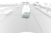
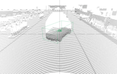
(a) Rotation failure cases 1

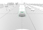
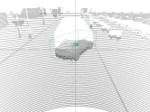
(b) Rotation failure cases 2

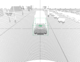
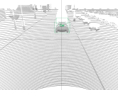
(c) Shifting failure cases

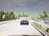
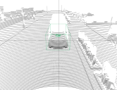
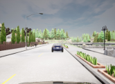
(d) Shifting failure cases

Figure 9: Rotation and shifting failure cases.

In this subsection, we present some failure cases and possible reasons.

As shown in Figure 9(a), where MonoCon fails to detect the front vehicle when the rotation angle $r$ is somewhere larger than $20^{\circ}$ but is able to detect it when $r\leq 20^{\circ}$, where CLOCs can detect cars with all rotation angles between $-30^{\circ}$ and $30^{\circ}$. The possible reason for this situation is that there are some objects (e.g. the puddle on the sidewalk and trees far away in this case) with similar color to the vehicle, which impacts the detection ability of camera-based detection modules. This problem can be mitigated by the LiDAR-based detection modules.

Figure 9(c) shows another failure case of camera-based models. Although there is no object with a similar color to the vehicle that we want to detect. The car farther is relatively small in the image, which is harder for camera-based models to detect. The application of point cloud data is very helpful in this case because of the perception ability of objects at long distances.

Figure 9(b) and Figure 9(d) shows two failure cases of SECOND, which is representative of LiDAR-based models where fusion models can detect relatively well. The possible reason for this case is that there are some objects very close to the vehicle (e.g.benches and grass in these cases), which affects the detection ability of point cloud modules, which can be mitigated by the combination with camera-based modules.

References

- [1] Vijay Badrinarayanan, Alex Kendall, and Roberto Cipolla. Segnet: A deep convolutional encoder-decoder architecture for image segmentation. IEEE transactions on pattern analysis and machine intelligence, 39(12):2481–2495, 2017.
- [2] Y. Cao, N. Wang, C. Xiao, D. Yang, J. Fang, R. Yang, Q. Chen, M. Liu, and B. Li. Invisible for both camera and lidar: Security of multi-sensor fusion based perception in autonomous driving under physical-world attacks. In 2021 IEEE Symposium on Security and Privacy (SP), pages 1302–1320, Los Alamitos, CA, USA, may 2021. IEEE Computer Society.
- [3] Nicholas Carlini, Florian Tramer, Krishnamurthy Dj Dvijotham, Leslie Rice, Mingjie Sun, and J Zico Kolter. (certified!!) adversarial robustness for free! In The Eleventh International Conference on Learning Representations, 2023.
- [4] Nicholas Carlini and David Wagner. Towards evaluating the robustness of neural networks. In 2017 ieee symposium on security and privacy (sp), pages 39–57. Ieee, 2017.
- [5] Xiaozhi Chen, Huimin Ma, Ji Wan, Bo Li, and Tian Xia. Multi-view 3d object detection network for autonomous driving. In Proceedings of the IEEE conference on Computer Vision and Pattern Recognition, pages 1907–1915, 2017.
- [6] Yukang Chen, Yanwei Li, Xiangyu Zhang, Jian Sun, and Jiaya Jia. Focal sparse convolutional networks for 3d object detection. In Proceedings of the IEEE/CVF Conference on Computer Vision and Pattern Recognition, pages 5428–5437, 2022.
- [7] Ping-yeh Chiang, Michael Curry, Ahmed Abdelkader, Aounon Kumar, John Dickerson, and Tom Goldstein. Detection as regression: Certified object detection with median smoothing. Advances in Neural Information Processing Systems, 33:1275–1286, 2020.
- [8] Wenda Chu, Linyi Li, and Bo Li. Tpc: Transformation-specific smoothing for point cloud models. In 39th International Conference on Machine Learning (ICML 2022), 2022.
- [9] Jeremy Cohen, Elan Rosenfeld, and Zico Kolter. Certified adversarial robustness via randomized smoothing. In International Conference on Machine Learning, pages 1310–1320. PMLR, 2019.
- [10] Jean-Emmanuel Deschaud. KITTI-CARLA: a KITTI-like dataset generated by CARLA Simulator. arXiv e-prints, 2021.
- [11] Alexey Dosovitskiy, German Ros, Felipe Codevilla, Antonio Lopez, and Vladlen Koltun. CARLA: An open urban driving simulator. In Proceedings of the 1st Annual Conference on Robot Learning, pages 1–16, 2017.
- [12] Logan Engstrom, Brandon Tran, Dimitris Tsipras, Ludwig Schmidt, and Aleksander Madry. Exploring the landscape of spatial robustness. In International conference on machine learning, pages 1802–1811. PMLR, 2019.
- [13] Kevin Eykholt, Ivan Evtimov, Earlence Fernandes, Bo Li, Amir Rahmati, Chaowei Xiao, Atul Prakash, Tadayoshi Kohno, and Dawn Song. Robust physical-world attacks on deep learning visual classification. In Proceedings of the IEEE conference on computer vision and pattern recognition, pages 1625–1634, 2018.
- [14] Amin Ghiasi, Ali Shafahi, and Tom Goldstein. Breaking certified defenses: Semantic adversarial examples with spoofed robustness certificates. In International Conference on Learning Representations, 2020.
- [15] Ian J Goodfellow, Jonathon Shlens, and Christian Szegedy. Explaining and harnessing adversarial examples. arXiv preprint arXiv:1412.6572, 2014.
- [16] Junyao Guo, Unmesh Kurup, and Mohak Shah. Is it safe to drive? an overview of factors, metrics, and datasets for driveability assessment in autonomous driving. IEEE Transactions on Intelligent Transportation Systems, 21(8):3135–3151, 2019.
- [17] R Spencer Hallyburton, Yupei Liu, Yulong Cao, Z Morley Mao, and Miroslav Pajic. Security analysis of camera-lidar fusion against black-box attacks on autonomous vehicles. In 31st USENIX Security Symposium (USENIX SECURITY), 2022.
- [18] Dan Hendrycks, Nicholas Carlini, John Schulman, and Jacob Steinhardt. Unsolved problems in ml safety. arXiv preprint arXiv:2109.13916, 2021.
- [19] Dan Hendrycks and Thomas Dietterich. Benchmarking neural network robustness to common corruptions and perturbations. In International Conference on Learning Representations, 2018.
- [20] Miklós Z. Horváth, Mark Niklas Mueller, Marc Fischer, and Martin Vechev. Boosting randomized smoothing with variance reduced classifiers. In International Conference on Learning Representations, 2022.
- [21] Hossein Hosseini and Radha Poovendran. Semantic adversarial examples. In Proceedings of the IEEE Conference on Computer Vision and Pattern Recognition Workshops, pages 1614–1619, 2018.
- [22] Qidong Huang, Xiaoyi Dong, Dongdong Chen, Hang Zhou, Weiming Zhang, Kui Zhang, Gang Hua, and Nenghai Yu. Pointcat: Contrastive adversarial training for robust point cloud recognition. arXiv preprint arXiv:2209.07788, 2022.
- [23] Mintong Kang, Linyi Li, Maurice Weber, Yang Liu, Ce Zhang, and Bo Li. Certifying some distributional fairness with subpopulation decomposition. In Alice H. Oh, Alekh Agarwal, Danielle Belgrave, and Kyunghyun Cho, editors, Advances in Neural Information Processing Systems, 2022.
- [24] Aounon Kumar, Alexander Levine, Soheil Feizi, and Tom Goldstein. Certifying confidence via randomized smoothing. Advances in Neural Information Processing Systems, 33:5165–5177, 2020.
- [25] Hei Law and Jia Deng. Cornernet: Detecting objects as paired keypoints. In Proceedings of the European conference on computer vision (ECCV), pages 734–750, 2018.
- [26] Linyi Li, Maurice Weber, Xiaojun Xu, Luka Rimanic, Bhavya Kailkhura, Tao Xie, Ce Zhang, and Bo Li. Tss: Transformation-specific smoothing for robustness certification. In Proceedings of the 2021 ACM SIGSAC Conference on Computer and Communications Security, pages 535–557, 2021.
- [27] Linyi Li, Tao Xie, and Bo Li. Sok: Certified robustness for deep neural networks. In 44th IEEE Symposium on Security and Privacy, SP 2023, San Francisco, CA, USA, 22-26 May 2023. IEEE, 2023.
- [28] Linyi Li, Jiawei Zhang, Tao Xie, and Bo Li. Double sampling randomized smoothing. In 39th International Conference on Machine Learning (ICML 2022), 2022.
- [29] Hang Liu and Wenlie Lei. Attack detection of localization based on multi-sensor fusion in autonomous systems. In 2022 IEEE International Conference on Unmanned Systems (ICUS), pages 1333–1338. IEEE, 2022.
- [30] Xianpeng Liu, Nan Xue, and Tianfu Wu. Learning auxiliary monocular contexts helps monocular 3d object detection. In Proceedings of the AAAI Conference on Artificial Intelligence, volume 36, pages 1810–1818, 2022.
- [31] Wenjie Luo, Bin Yang, and Raquel Urtasun. Fast and furious: Real time end-to-end 3d detection, tracking and motion forecasting with a single convolutional net. In Proceedings of the IEEE conference on Computer Vision and Pattern Recognition, pages 3569–3577, 2018.
- [32] Aleksander Madry, Aleksandar Makelov, Ludwig Schmidt, Dimitris Tsipras, and Adrian Vladu. Towards deep learning models resistant to adversarial attacks. In International Conference on Learning Representations, 2018.
- [33] Phil McCausland. Self-driving uber car that hit and killed woman did not recognize that pedestrians jaywalk, Nov 2019.
- [34] Su Pang, Daniel Morris, and Hayder Radha. Clocs: Camera-lidar object candidates fusion for 3d object detection. In 2020 IEEE/RSJ International Conference on Intelligent Robots and Systems (IROS), pages 10386–10393. IEEE, 2020.
- [35] Kexin Pei, Yinzhi Cao, Junfeng Yang, and Suman Jana. Deepxplore: Automated whitebox testing of deep learning systems. In proceedings of the 26th Symposium on Operating Systems Principles, pages 1–18, 2017.
- [36] Charles R Qi, Wei Liu, Chenxia Wu, Hao Su, and Leonidas J Guibas. Frustum pointnets for 3d object detection from rgb-d data. In Proceedings of the IEEE conference on computer vision and pattern recognition, pages 918–927, 2018.
- [37] Joseph Redmon, Santosh Divvala, Ross Girshick, and Ali Farhadi. You only look once: Unified, real-time object detection. In Proceedings of the IEEE conference on computer vision and pattern recognition, pages 779–788, 2016.
- [38] Shaoqing Ren, Kaiming He, Ross Girshick, and Jian Sun. Faster r-cnn: Towards real-time object detection with region proposal networks. Advances in neural information processing systems, 28, 2015.
- [39] Hadi Salman, Jerry Li, Ilya Razenshteyn, Pengchuan Zhang, Huan Zhang, Sebastien Bubeck, and Greg Yang. Provably robust deep learning via adversarially trained smoothed classifiers. In H. Wallach, H. Larochelle, A. Beygelzimer, F. d'Alché-Buc, E. Fox, and R. Garnett, editors, Advances in Neural Information Processing Systems, volume 32. Curran Associates, Inc., 2019.
- [40] Pouya Samangouei, Maya Kabkab, and Rama Chellappa. Defense-gan: Protecting classifiers against adversarial attacks using generative models. In International Conference on Learning Representations, 2018.
- [41] Ali Shafahi, Mahyar Najibi, Mohammad Amin Ghiasi, Zheng Xu, John Dickerson, Christoph Studer, Larry S Davis, Gavin Taylor, and Tom Goldstein. Adversarial training for free! Advances in Neural Information Processing Systems, 32, 2019.
- [42] Junjie Shen, Ningfei Wang, Ziwen Wan, Yunpeng Luo, Takami Sato, Zhisheng Hu, Xinyang Zhang, Shengjian Guo, Zhenyu Zhong, Kang Li, et al. Sok: On the semantic ai security in autonomous driving. arXiv preprint arXiv:2203.05314, 2022.
- [43] Sahil Singla and Soheil Feizi. Skew orthogonal convolutions. In International Conference on Machine Learning, pages 9756–9766. PMLR, 2021.
- [44] Jiachen Sun, Yulong Cao, Qi Alfred Chen, and Z Morley Mao. Towards robust lidar-based perception in autonomous driving: General black-box adversarial sensor attack and countermeasures. In USENIX Security Symposium (Usenix Security’20), 2020.
- [45] Jiachen Sun, Akshay Mehra, Bhavya Kailkhura, Pin-Yu Chen, Dan Hendrycks, Jihun Hamm, and Z Morley Mao. A spectral view of randomized smoothing under common corruptions: Benchmarking and improving certified robustness. In Computer Vision–ECCV 2022: 17th European Conference, Tel Aviv, Israel, October 23–27, 2022, Proceedings, Part IV, pages 654–671. Springer, 2022.
- [46] Christian Szegedy, Wojciech Zaremba, Ilya Sutskever, Joan Bruna, Dumitru Erhan, Ian Goodfellow, and Rob Fergus. Intriguing properties of neural networks. arXiv preprint arXiv:1312.6199, 2013.
- [47] Eric Wong and Zico Kolter. Provable defenses against adversarial examples via the convex outer adversarial polytope. In International Conference on Machine Learning, pages 5286–5295. PMLR, 2018.
- [48] Chaowei Xiao, Jun-Yan Zhu, Bo Li, Warren He, Mingyan Liu, and Dawn Song. Spatially transformed adversarial examples. In International Conference on Learning Representations, 2018.
- [49] Xiaojun Xu, Linyi Li, and Bo Li. Lot: Layer-wise orthogonal training on improving l2 certified robustness. In Advances in Neural Information Processing Systems 35 (NeurIPS 2022), 2022.
- [50] Yan Yan, Yuxing Mao, and Bo Li. Second: Sparsely embedded convolutional detection. Sensors, 18(10):3337, 2018.
- [51] Greg Yang, Tony Duan, J Edward Hu, Hadi Salman, Ilya Razenshteyn, and Jerry Li. Randomized smoothing of all shapes and sizes. In International Conference on Machine Learning, pages 10693–10705. PMLR, 2020.
- [52] Bohang Zhang, Du Jiang, Di He, and Liwei Wang. Rethinking lipschitz neural networks and certified robustness: A boolean function perspective. In Advances in Neural Information Processing Systems, 2022.
- [53] Huan Zhang, Shiqi Wang, Kaidi Xu, Linyi Li, Bo Li, Suman Jana, Cho-Jui Hsieh, and J. Zico Kolter. General cutting planes for bound-propagation-based neural network verification. In Advances in Neural Information Processing Systems 35 (NeurIPS 2022), 2022.
- [54] Hengshuang Zhao, Xiaojuan Qi, Xiaoyong Shen, Jianping Shi, and Jiaya Jia. Icnet for real-time semantic segmentation on high-resolution images. In Proceedings of the European conference on computer vision (ECCV), pages 405–420, 2018.
- [55] Ziyuan Zhong, Zhisheng Hu, Shengjian Guo, Xinyang Zhang, Zhenyu Zhong, and Baishakhi Ray. Detecting multi-sensor fusion errors in advanced driver-assistance systems. In Proceedings of the 31st ACM SIGSOFT International Symposium on Software Testing and Analysis, pages 493–505, 2022.
- [56] Yin Zhou and Oncel Tuzel. Voxelnet: End-to-end learning for point cloud based 3d object detection. In Proceedings of the IEEE conference on computer vision and pattern recognition, pages 4490–4499, 2018.