Effective extensional-torsional elasticity and dynamics of helical filaments under distributed loads

Abstract

We study slender, helical elastic rods subject to distributed forces and moments. Focussing on the case when the helix axis remains straight, we employ the method of multiple scales to systematically derive an ‘effective-column’ theory from the Kirchhoff rod equations: the helical filament is described as a naturally-straight rod (aligned with the helix axis) for which the extensional and torsional deformations are coupled. Importantly, our analysis is asymptotically exact in the limit of a ‘highly-coiled’ filament (i.e., when the helical wavelength is much smaller than the characteristic lengthscale over which the filament bends due to external loading) and is able to account for large, unsteady displacements. In the small-deformation limit, we exactly recover the coupled wave equations used to describe the free vibrations of helical coil springs, thereby justifying previous effective-column approximations in which linearised stiffness coefficients are assumed to apply locally and dynamically. We then illustrate our theory with two loading scenarios: (I) a heavy helical rod deforming under its own weight; and (II) the dynamics of axial rotation (twirling) in viscous fluid, which may be considered as a simple model for a bacteria flagellar filament. More broadly, our analysis provides a framework to develop reduced models of helical rods in a wide variety of physical and biological settings, and yields analytical insight into their elastic instabilities. In particular, our analysis indicates that tensile instabilities are a generic phenomenon when helical rods are subject to a combination of distributed forces and moments.

1 Introduction

1.1 Background

Slender elastic rods (also known as ‘filaments’) with an intrinsic helical geometry are encountered in a wide range of physical and biological systems. In engineering, helical coil springs have long been used to store energy and absorb shock, with applications ranging from computer keyboards and mattresses to vehicle suspension systems (Kobelev, 2021). In biology, helical forms appear in a variety of settings, including the tendrils of climbing plants (McMillen and Goriely, 2002), arteries and veins in the human umbilical cord (Malpas and Symonds, 1966), the shape of some viruses (Stubbs and Kendall, 2012), and — perhaps most famous of all — DNA, a biopolymer comprising two helical strands of nucleic acid that spiral around one another (Watson and Crick, 1953). Furthermore, the majority of bacteria are propelled by helical filaments whose rotation in a viscous fluid induces forward propulsion due to their chiral shape (Lauga, 2020). Recent interest in artificial swimmers has seen the design of bio-inspired devices driven by helical filaments (Zhang et al., 2009; Katsamba and Lauga, 2019; Huang et al., 2019; Lim et al., 2023).

In these systems, the elasticity of the filament often plays a key role in its function. Indeed, the flexibility of a traditional coil spring is essential for its ability to absorb energy, and the linear relationship between small longitudinal displacements of a spring and the applied force serves as the paradigmatic example of Hooke’s Law. Similarly, the elasticity of biofilaments often plays an important role. For example, the variety of polymeric filaments (from actin to microtubules) inside the cytoskeleton of cells have a range of bending rigidities tuned to their structural functions in the cells (Howard, 2001). The flexibility of DNA is known to be necessary for a variety of processes including replication, packing inside eukaryotic nuclei, and binding to proteins (Peters and Maher, 2010; Marin-Gonzalez et al., 2021). Moreover, the run-and-tumble motion of multi-flagellated bacteria (such as E. coli) requires that the flagellar filaments are sufficiently flexible to form a tight bundle behind the cell body during steady swimming, yet stiff enough to unbundle once one of the rotary motors slows down or reverses direction (Berg, 2003, 2004; Riley et al., 2018).

To model the elastic deformations and dynamics of helical filaments, the Kirchhoff rod equations are commonly used (Goriely and Tabor, 1997c; Goriely, 2017). These equations are geometrically nonlinear and so can account for large, global displacements of the rod in three dimensions, while maintaining a mechanically-linear (i.e., Hookean) constitutive law; such large displacements are consistent with the assumption of small local strains, as required for linear elasticity, provided that the lengthscale of the deformation is much larger than the cross-section dimensions of the rod (Audoly and Pomeau, 2010). This geometric nonlinearity also makes a mathematical analysis of the rod equations difficult, so that the dynamic behaviour of helical rods under external loading is still generally poorly understood. Most research in the area tends to be computational in nature (Shum and Gaffney, 2012; Jawed et al., 2015; Jawed and Reis, 2017; Park et al., 2017, 2019), though simulations are computationally expensive due to the inherent three-dimensional geometry of helical filaments, meaning only a relatively small number of simulations may feasibly be performed. One alternative approach is to use a coarse-grained elastic model — for example, by replacing the filament by bead-spring interactions — to decrease the computational expense. Coarse-grained models have been applied successfully to study flagellar bundling (Flores et al., 2005; Watari and Larson, 2010; Nguyen and Graham, 2017, 2018) and the stability of a Slinky toy (Holmes et al., 2014), although such models are generally still too complex to be solved analytically.

As an alternative to numerical simulations, analytical models are of fundamental importance: they clarify the dependence on (possibly many) parameters of a system, and provide a basis to guide more detailed simulations or experiments. In general, to make analytical progress with the Kirchhoff rod equations an approximation must be made, for which previous work can roughly be split into two groups. The first group is based on the assumption that the filament is relatively stiff compared to the external loads, or close to a buckling threshold, so that the deformed shape can be analysed as a small perturbation away from a known base state (such as the natural helical shape). Early work considered helices of small pitch angle and treated the natural shape as a small perturbation from a straight rod (Haringx, 1949). Goriely and Tabor (1997a) and Goriely and Tabor (1997b) developed a general perturbation scheme to study, respectively, the linear stability and weakly-nonlinear dynamics of elastic rods; this scheme was then applied to helical rods by Goriely and Tabor (1997c), who quantified the early-time dynamics of buckling under axial compression. Moreover, the assumption of small deformations is useful when modelling helices rotating in viscous fluid, since the fluid and elastic problems can be decoupled to a first approximation: the viscous drag is computed for an undeformed helix rigidly rotating about its axis, and this drag is then used to calculate the deformed shape (Takano et al., 2003; Kim and Powers, 2005). This asymptotic procedure was explored in detail by Katsamba and Lauga (2019), who were also able to calculate the next-order correction to the drag forces in this approximation.

The second group of analytical models consists of ‘effective-column’ approximations, which have long been used in engineering to describe the deformations and vibrations of helical springs; see Chapter $3$ of Kobelev (2021) and references therein. These model the helical filament as a naturally-straight beam (or column) whose centreline is aligned with the helix axis; the effective elastic properties of the beam are chosen so that the deformation captures that of the full helix in simple loading situations, for example end-to-end compression or uniform bending. In the absence of distributed loads, a theoretical basis for an effective-column approximation is provided by the work of Love (1944), who derived equilibrium equations for helical filaments based on the inextensible Kirchhoff rod equations under terminal loads. In the case where the loads form a wrench whose axis coincides with the axis of the helix, an exact solution of these equations is that of another helix with modified geometry (Love, 1944). By linearising this solution in the limit of small deformations, stiffness coefficients for an effective-column approximation can be obtained. Using an ad hoc assumption that these linearised stiffness coefficients can be applied locally (i.e., for each infinitesimal spring element) in dynamic problems, Phillips and Costello (1972) analysed the free vibrations of helical springs, obtaining good agreement with experiments even for large longitudinal displacements. This work has since been extended, for example to address the radial expansion of impacted springs (Costello, 1975), filament extensibility (Jiang et al., 1991; Jiang and Wang, 1998), and the effects of shear deformations (Krużelecki and Życzkowski, 1990; Michalczyk and Bera, 2019). However, the validity of effective-column approximations remains unclear when dynamic effects and distributed loads are present.

Effective-column models have also been developed in other contexts, including models for highly-twisted biofilaments. Kehrbaum and Maddocks (2000) analysed the mechanical properties of an elastic rod with high intrinsic twist, as a model for DNA molecules deforming over lengthscales much larger than that of individual base pairs. Using a Hamiltonian formulation of the Kirchhoff rod equations in the absence of distributed loads, in which the twist lengthscale plays the role of a ‘fast’ time-like variable in a dynamical system, they used homogenisation techniques to obtain an effective constitutive law governing bending over relatively large or ‘slow’ lengthscales. Rey and Maddocks (2000) built upon this work to consider twisted rods under general boundary conditions and buckling under compression.

There are several hints that a similar averaged theory may be fruitful to describe the mechanics of helical filaments when distributed loads are present. For example, the instabilities of a helical rod rotating in viscous fluid share many features with those of a naturally-straight rod. If a naturally-straight rod is rotated about its axis while the other end is free, the straight (twirling) state undergoes a Hopf bifurcation at a critical frequency to a whirling state characterised by significant bending (Wolgemuth et al., 2000). A helical rod (with sufficiently shallow pitch angle) rotated about its axis exhibits an analogous instability, for which the critical frequency scales with the bending stiffness and filament length identically to the straight-rod case (Park et al., 2017). At large pitch angles, the translation-rotation coupling in the viscous drag becomes significant and the filament may buckle under a combination of the hydrodynamic torque and propulsive force. In this regime, Vogel and Stark (2012) were able to obtain good agreement with a straight-rod model and Jawed et al. (2015) found that the critical frequency scales identically to an effective beam of equal length.

1.2 Summary and structure of this paper

In this paper, we develop a reduced model for a helical rod undergoing unsteady deformations in the presence of distributed forces and moments. The fundamental assumptions of our theory are that (i) the helix wavelength is much smaller than the characteristic lengthscale over which the filament bends (we refer to this as the ‘highly-coiled’ assumption); (ii) the filament is sufficiently slender so that the local strains remain small and we may assume linear elasticity; (iii) the filament has uniform, circular cross-section; and (iv) the helix axis remains straight. While in general multiple types of deformation are possible, namely extensional-rotational deformations about the helix axis and bending of the helix axis itself, we ignore axis bending here as it allows us to understand how the helical geometry depends on the distributed loads without introducing additional complexity.

Inspired by the work of Kehrbaum and Maddocks (2000) and Rey and Maddocks (2000) on straight rods with high intrinsic twist, we employ a homogenisation procedure in which the helix wavelength acts as a ‘fast’ time-like variable. The basis of our method is Love’s helical solution of the Kirchhoff rod equations, in the case of a constant wrench aligned with the helix axis (Love, 1944). Under the highly-coiled assumption, the force and moment resultants in the rod are approximately constant over each helical wavelength; provided that the helix axis remains straight, these resultants form a wrench aligned with the helix axis, so that the solution is locally a rigid transformation of a helix with modified geometric parameters. We then apply the method of multiple scales to describe ‘slow’ variations in the geometric parameters under distributed loading. These variations in helical geometry correspond to extensional and torsional deformations about the helix axis, so that we obtain an effective-column theory.

The remainder of this paper is organised as follows. In §2, we present the Kirchhoff rod equations and their non-dimensionalisation, before introducing the highly-coiled assumption. In §3, we apply the method of multiple scales to derive the effective-column equations, showing how these arise as solvability conditions on an appropriate first-order problem when the solution is expanded as an asymptotic series. In §4, we analyse the effective-column equations in detail: we first show how the equations can be written in terms of useful pairs of variables for analysis, before considering singularities and the small-deformation limit of the equations. We next apply our results to two specific scenarios: the compression/extension of a heavy helical column in §5, and the dynamics of a helix rotating in viscous fluid in §6. Finally, in §7, we summarise our findings and conclude. We discuss how the framework introduced here may be extended to incorporate other effects, including axis bending and different cross-section shapes, and we comment on the physical significance of singularities for instabilities of helical rods subject to distributed loads.

2 Theoretical formulation

In this section we derive the equations governing the helical filament in the framework of Kirchhoff rod theory. We present only the key ingredients here; for a detailed treatment see Audoly and Pomeau (2010) or Goriely (2017). We consider an elastic filament whose undeformed centreline is a uniform helix with contour length $l$, pitch angle $\alpha^{u}$ (the angle between the centreline tangent and the helix axis), contour wavelength $\lambda^{u}$, and chirality index $h=\pm 1$ ($h=-1$ or $+1$ corresponds, respectively, to a left-handed or a right-handed helix); see Fig. 1a. Simple geometry states that the radius of the cylinder on which the helix is wound is $r^{u}=\lambda^{u}\sin\alpha^{u}/(2\pi)$. Here and throughout this paper, we use the superscript ^u to denote quantities of the undeformed shape that may change during deformation, and drop these for the deformed (current) shape. The filament has a circular cross-section of constant radius $a$ and we assume that it is sufficiently slender (i.e., $a\ll\lambda^{u}$) so that it is inextensible and unshearable. We also assume that the filament is composed of a uniform, isotropic material of density $\rho_{s}$ and that the strains remain small; we may then use a linearly elastic constitutive law with (constant) Young’s modulus $E$ and Poisson ratio $\nu$.

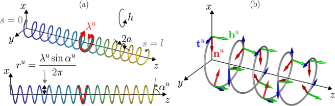
Figure 1: (a) Schematic diagram of the undeformed helical filament, showing the notation we use: total contour length $l$, pitch angle $\alpha^{u}$, chirality index $h$, contour wavelength $\lambda^{u}$, helix radius $r^{u}$, filament radius $a$, arclength $s$ and Cartesian coordinates $(x,y,z)$ (the helix frame). (b) Corresponding Frenet-Serret basis vectors.

2.1 Kinematics

As shown in Fig. 1a, we introduce Cartesian coordinates $Oxyz$ (the ‘helix frame’) such that the undeformed helix axis lies on the $z$-axis, and the filament base (taken to be at $z=0$) lies on the $x$-axis. The corresponding unit Cartesian vectors are denoted $\{\mathbf{e}_{x},\mathbf{e}_{y},\mathbf{e}_{z}\}$. If the filament base is not fixed in space but is allowed to move (e.g., if it is attached to a freely-moving body), the helix frame rotates and translates relative to the laboratory frame.

Deformed configuration

During deformation, we write $\mathbf{r}(s,t)$ for the centreline position at arclength $s$ (measured from the filament base) and time $t$. Under the inextensibility assumption, the unit tangent vector, $\mathbf{d}_{3}(s,t)$, is

$$\mathbf{d}_{3}=\frac{\partial\mathbf{r}}{\partial s},$$ (1)

which we refer to as the inextensibility constraint. To describe the local orientation of the rod, we introduce the additional vectors $\mathbf{d}_{1}(s,t)$ and $\mathbf{d}_{2}(s,t)$ such that $\{\mathbf{d}_{1},\mathbf{d}_{2},\mathbf{d}_{3}\}$ (referred to as directors) form a right-handed orthonormal basis for each $s$ and $t$; the vectors $\{\mathbf{d}_{1},\mathbf{d}_{2}\}$ span the normal plane through the cross-section, changing orientation as the rod bends and twists. We can then quantify mechanical strains via the strain vector, $\mathbf{u}$, and angular velocity vector, $\boldsymbol{\omega}$ (also known as the twist vector and spin vector, respectively; see Goriely and Tabor, 1997c), which account for rotations of the directors as $s$ or $t$ varies (hence preserving their orthonormality):

$$\frac{\partial\mathbf{d}_{i}}{\partial s}=\mathbf{u}\times\mathbf{d}_{i},\quad\frac{\partial\mathbf{d}_{i}}{\partial t}=\boldsymbol{\omega}\times\mathbf{d}_{i},\qquad i=1,2,3.$$ (2)

Expressing $\mathbf{u}$ and $\boldsymbol{\omega}$ in terms of components with respect to the director basis,

$$\mathbf{u}=u_{1}\mathbf{d}_{1}+u_{2}\mathbf{d}_{2}+u_{3}\mathbf{d}_{3},\quad\boldsymbol{\omega}=\omega_{1}\mathbf{d}_{1}+\omega_{2}\mathbf{d}_{2}+\omega_{3}\mathbf{d}_{3},$$

we can interpret $u_{1}$ and $u_{2}$ as the bending strains (the rate at which the tangent vector $\mathbf{d}_{3}$ rotates about $\mathbf{d}_{1}$ and $\mathbf{d}_{2}$, respectively, as $s$ increases) and $u_{3}$ as the twist strain (the rate at which $\mathbf{d}_{1}$ and $\mathbf{d}_{2}$ rotate about $\mathbf{d}_{3}$, which incorporates both axial twist and centreline torsion) (Audoly and Pomeau, 2010). The interpretation of the components $\omega_{i}$ is analogous with $s$ replaced by time, $t$.

Undeformed configuration

The undeformed centreline can be written in cylindrical polar coordinates as

$$\mathbf{r}^{u}(s)=r^{u}\,\mathbf{e}_{r}(s)+s\cos\alpha^{u}\,\mathbf{e}_{z},\qquad 0<s<l,$$ (3)

where the local unit vectors, evaluated on the centreline, and the winding angle of the helix (i.e., the polar angle between the radius to the filament and the $x$-axis) are

$$\mathbf{e}_{r}(s)=\cos\Psi^{u}(s)\,\mathbf{e}_{x}+\sin\Psi^{u}(s)\,\mathbf{e}_{y},\quad\mathbf{e}_{\theta}(s)=-\sin\Psi^{u}(s)\,\mathbf{e}_{x}+\cos\Psi^{u}(s)\,\mathbf{e}_{y},\qquad\Psi^{u}(s)=\frac{2\pi hs}{\lambda^{u}}.$$ (4)

Without loss of generality, we choose the undeformed director basis to coincide with the Frenet-Serret frame $\{\mathbf{n}^{u},\mathbf{b}^{u},\mathbf{t}^{u}\}$; here $\mathbf{n}^{u}$, $\mathbf{b}^{u}$ and $\mathbf{t}^{u}$ correspond to the unit normal, binormal and tangent vectors along $\mathbf{r}^{u}(s)$, respectively:

$$\mathbf{n}^{u}(s)=-\mathbf{e}_{r}(s),\quad\mathbf{b}^{u}(s)=-\cos\alpha^{u}\,\mathbf{e}_{\theta}(s)+h\sin\alpha^{u}\,\mathbf{e}_{z},\quad\mathbf{t}^{u}(s)=h\sin\alpha^{u}\,\mathbf{e}_{\theta}(s)+\cos\alpha^{u}\,\mathbf{e}_{z}.$$ (5)

These are shown in Fig. 1b. Setting $\{\mathbf{d}_{1},\mathbf{d}_{2},\mathbf{d}_{3}\}=\{\mathbf{n}^{u},\mathbf{b}^{u},\mathbf{t}^{u}\}$ in Eq. (2) shows that the undeformed strain vector, denoted $\mathbf{u}^{u}$, is equal to the Darboux vector of the Frenet-Serret frame:

$$\mathbf{u}^{u}=\kappa^{u}\mathbf{b}^{u}+\tau^{u}\mathbf{t}^{u}=\frac{2\pi h}{\lambda^{u}}\mathbf{e}_{z}\qquad\mathrm{where}\qquad\kappa^{u}=\frac{2\pi\sin\alpha^{u}}{\lambda^{u}},\quad\tau^{u}=\frac{2\pi h\cos\alpha^{u}}{\lambda^{u}}.$$ (6)

The quantities $\kappa^{u}$ and $\tau^{u}$ are the Frenet curvature and torsion of $\mathbf{r}^{u}$, respectively.

2.2 Mechanics

Let $\mathbf{f}(s,t)$ be the resultant force and $\mathbf{m}(s,t)$ be the resultant moment attached to the filament centreline, obtained by averaging the internal elastic stresses over the cross-section at position $s$. Balancing linear and angular momentum, we obtain the inextensible, unshearable Kirchhoff rod equations (Audoly and Pomeau, 2010)

$$\frac{\partial\mathbf{f}}{\partial s}+\mathbf{f}_{e}=\rho_{s}A\frac{\partial^{2}\mathbf{r}}{\partial t^{2}},$$ (7)

$$\frac{\partial\mathbf{m}}{\partial s}+\mathbf{d}_{3}\times\mathbf{f}+\mathbf{m}_{e}=\rho_{s}I\left(\mathbf{d}_{1}\times\frac{\partial^{2}\mathbf{d}_{1}}{\partial t^{2}}+\mathbf{d}_{2}\times\frac{\partial^{2}\mathbf{d}_{2}}{\partial t^{2}}\right),$$ (8)

where $\mathbf{f}_{e}$ and $\mathbf{m}_{e}$ are, respectively, the external force and moment exerted on the rod per unit arclength, $A=\pi a^{2}$ is the cross-sectional area, and $I=\pi a^{4}/4$ is the second moment of area of the cross-section. (We neglect fictitious forces that may arise when the helix frame is non-inertial and accelerates relative to the laboratory frame.) The above equations are supplemented with the isotropic, Hookean (linearly elastic) constitutive law

$$\mathbf{m}=B\left[u_{1}\mathbf{d}_{1}+\left(u_{2}-\kappa^{u}\right)\mathbf{d}_{2}\right]+C\left(u_{3}-\tau^{u}\right)\mathbf{d}_{3},$$ (9)

where $B=EI$ is the bending modulus and $C=\mu_{s}J$ is the twist modulus ($\mu_{s}=E/[2(1+\nu)]$ is the shear modulus and $J$ is the torsion constant) (Howell et al., 2009). We neglect warping of the cross-section (justified by its circular shape), which gives $J=2I=\pi a^{4}/2$ and hence

$$C=\frac{B}{1+\nu}.$$ (10)

The appearance of $\kappa^{u}$ and $\tau^{u}$ in Eq. (9) guarantees that the rod is unstressed in its undeformed shape when $\{\mathbf{d}_{1},\mathbf{d}_{2},\mathbf{d}_{3}\}=\{\mathbf{n}^{u},\mathbf{b}^{u},\mathbf{t}^{u}\}$ and $\mathbf{u}=\mathbf{u}^{u}=\kappa^{u}\mathbf{b}^{u}+\tau^{u}\mathbf{t}^{u}$.

2.3 Boundary conditions

Given the external forces and moments, the system is closed by appropriate boundary conditions and (if relevant) initial conditions. We shall restrict to situations where the filament tip $s=l$ remains free of forces and moments:

$$\mathbf{f}(l,t)=\mathbf{m}(l,t)=\mathbf{0}.$$ (11)

In general, it is also necessary to provide boundary conditions at the filament base, for example specifying the position and orientation of the filament. However, the multiple-scales analysis presented in §3 leads to effective-column equations that are first-order in space, so that the boundary conditions (11) uniquely specify the solution (assuming the external forces and moments are known). To be compatible with the effective-column approximation, we therefore suppose that the filament is supported at its base such that the centreline is located on the $x$-axis in the $z=0$ plane; this is equivalent to the condition

$$\mathbf{r}(0,t)\times\mathbf{e}_{x}=\mathbf{0}.$$ (12)

At leading order, we thus do not specify the orientation of the filament nor its $x$-coordinate at $z=0$. Once the effective-column equations are solved, the value of $\mathbf{r}(0,t)$ is determined and hence the centreline $\mathbf{r}(s,t)$ can be found by integrating the inextensibility constraint (1).

2.4 Non-dimensionalisation

To non-dimensionalise the problem, it is natural to scale all lengths by the undeformed helical wavelength, $\lambda^{u}$. From the kinematic equations (2), the strain vector scales as $|\mathbf{u}|\sim 1/\lambda^{u}$. We scale the moment and force resultants by their typical magnitudes associated with bending over the lengthscale $\lambda^{u}$. Using the constitutive law (9) and moment balance (8), these are $|\mathbf{m}|\sim B/\lambda^{u}$ and $|\mathbf{f}|\sim B/({\lambda^{u}})^{2}$. We denote the typical magnitudes of the external force and moment by $[f]$ and $[m]$, respectively, which are determined by the physics governing the external loading. Keeping the timescale $[t]$ unspecified for now, we then introduce the dimensionless variables

$$\mathbf{r}=\lambda^{u}\mathbf{R},\quad (x,y,z,s)=\lambda^{u}(X,Y,Z,S),\quad l=\lambda^{u}L,\quad(\kappa^{u},\tau^{u})=\frac{1}{\lambda^{u}}(\mathcal{K}^{u},\mathcal{T}^{u}),\quad\mathbf{u}=\frac{1}{\lambda^{u}}\mathbf{U},\quad\mathbf{u}^{u}=\frac{1}{\lambda^{u}}\mathbf{U}^{u},\quad u_{i}=\frac{1}{\lambda^{u}}U_{i},$$

$$t=[t]T,\quad\boldsymbol{\omega}=\frac{1}{[t]}\boldsymbol{\Omega},\quad\omega_{i}=\frac{1}{[t]}\Omega_{i},\quad\mathbf{m}=\frac{B}{\lambda^{u}}\mathbf{M},\quad\mathbf{f}=\frac{B}{({\lambda^{u}})^{2}}\mathbf{F},\quad\mathbf{f}_{e}=[f]\mathbf{F}_{e},\quad\mathbf{m}_{e}=[m]\mathbf{M}_{e}.$$ (13)

Under the above re-scalings, the inextensibility constraint (1) becomes

$$\mathbf{d}_{3}=\frac{\partial\mathbf{R}}{\partial S}.$$ (14)

In terms of the dimensionless strain vector $\mathbf{U}=\sum_{i}U_{i}\mathbf{d}_{i}$ and angular velocity vector $\boldsymbol{\Omega}=\sum_{i}\Omega_{i}\mathbf{d}_{i}$, the kinematic equations (2) are

$$\frac{\partial\mathbf{d}_{i}}{\partial S}=\mathbf{U}\times\mathbf{d}_{i},\quad\frac{\partial\mathbf{d}_{i}}{\partial T}=\boldsymbol{\Omega}\times\mathbf{d}_{i},\qquad i=1,2,3.$$ (15)

Using Eq. (3), the dimensionless natural shape, $\mathbf{R}^{u}=\mathbf{r}^{u}/\lambda^{u}$, can be written as

$$\mathbf{R}^{u}(S)=\frac{\sin\alpha^{u}}{2\pi}\mathbf{e}_{r}(S)+S\cos\alpha^{u}\,\mathbf{e}_{z},\qquad 0<S<L.$$ (16)

In terms of dimensionless arclength, $S$, the undeformed winding angle is written $\Psi^{u}(S)=2\pi hS$. Using Eq. (6), the dimensionless undeformed strain vector, Frenet curvature and torsion are

$$\mathbf{U}^{u}=\mathcal{K}^{u}\mathbf{b}^{u}+\mathcal{T}^{u}\mathbf{t}^{u}=2\pi h\mathbf{e}_{z},\quad\mathcal{K}^{u}=2\pi\sin\alpha^{u},\quad\mathcal{T}^{u}=2\pi h\cos\alpha^{u}.$$ (17)

The force and moment balances (7)–(8) now read

$$\frac{\partial\mathbf{F}}{\partial S}+\epsilon\,\mathbf{F}_{e}=\left(\frac{{t^{*}}}{[t]}\right)^{2}\frac{\partial^{2}\mathbf{R}}{\partial T^{2}},$$ (18)

$$\frac{\partial\mathbf{M}}{\partial S}+\mathbf{d}_{3}\times\mathbf{F}+\epsilon\,\delta\,\mathbf{M}_{e}=\eta^{2}\left(\frac{{t^{*}}}{[t]}\right)^{2}\left(\mathbf{d}_{1}\times\frac{\partial^{2}\mathbf{d}_{1}}{\partial T^{2}}+\mathbf{d}_{2}\times\frac{\partial^{2}\mathbf{d}_{2}}{\partial T^{2}}\right),$$ (19)

where we define

$$\epsilon=\frac{({\lambda^{u}})^{3}[f]}{B},\quad\delta=\frac{[m]}{[f]\lambda^{u}},\quad t^{*}=\sqrt{\frac{\rho_{s}A(\lambda^{u})^{4}}{B}},\quad\eta=\frac{\sqrt{I/A}}{\lambda^{u}}.$$ (20)

Here $\epsilon$ and $\delta$ are dimensionless parameters measuring the relative importance of the external force and moment, respectively; $t^{*}$ is the timescale of inertial oscillations on the wavelength lengthscale; and $\eta$ is a slenderness parameter. Using $A=\pi a^{2}$ and $I=\pi a^{4}/4$, we have $\eta=a/(2\lambda^{u})$; consistent with neglecting the effects of axial extensibility in the limit $a\ll\lambda^{u}$, we neglect the $\eta^{2}$ term on the right-hand side of Eq. (19) so that the moment balance simplifies to

$$\frac{\partial\mathbf{M}}{\partial S}+\mathbf{d}_{3}\times\mathbf{F}+\epsilon\,\delta\,\mathbf{M}_{e}=\mathbf{0}.$$ (21)

We will assume that $\delta=O(1)$, i.e., the deformation is driven mainly by the external force in Eq. (18) (though this assumption is not essential and the averaging method we present in §3 may be readily adapted to the case when the deformation is instead driven by the external moment).

We write the force and moment resultants in terms of components with respect to the director basis, $\mathbf{F}=\sum_{i}F_{i}\mathbf{d}_{i}$ and $\mathbf{M}=\sum_{i}M_{i}\mathbf{d}_{i}$. Using Eq. (10), the constitutive law (9) becomes

$$M_{1}=U_{1},\quad M_{2}=U_{2}-\mathcal{K}^{u},\quad M_{3}=\frac{U_{3}-\mathcal{T}^{u}}{1+\nu}.$$ (22)

Finally, the boundary conditions (11)–(12) become

$$\mathbf{R}(0,T)\times\mathbf{e}_{x}=\mathbf{0},\quad\mathbf{F}(L,T)=\mathbf{M}(L,T)=\mathbf{0}.$$ (23)

For unsteady problems, the relevant initial conditions are non-dimensionalised to complete the system.

2.5 Highly-coiled assumption

The fundamental ‘highly-coiled’ assumption that we make in this paper is that the impact of the external loading is small on the wavelength lengthscale, i.e. we assume that $\epsilon\ll 1$. Note from (20) that $\epsilon$ can be written as

$$\epsilon=\left(\frac{\lambda^{u}}{[s]}\right)^{3},$$

where $[s]=(B/[f])^{1/3}$ is a deformation lengthscale that can be interpreted as the typical contour length over which the filament bends significantly due to the external force density $[f]$ (in particular, $[s]$ can be obtained by balancing terms in the force balance (7) using the scaling behaviour $|\mathbf{f}|\sim B/[s]^{2}$ and $\partial/\partial s\sim 1/[s]$). The highly-coiled assumption $\epsilon\ll 1$ then states that $\lambda^{u}\ll[s]$, i.e., there is negligible bending over each helical wavelength. In the next section, we show how this assumption can be exploited to construct an effective-column theory for the filament.

3 Multiple-scales analysis of highly-coiled filaments

In the limit of highly-coiled filaments ($\epsilon\ll 1$), we anticipate an approximate solution using the method of multiple scales, in which arclength is analogous to the time variable in a dynamical system. On the ‘fast’ wavelength lengthscale, $S=O(1)$, the force and moment resultants are approximately constant. Provided that the helix axis remains straight, these resultants form a wrench aligned with the helix axis, and a stationary solution to the Kirchhoff rod equations is another helix with (in general) modified pitch angle and wavelength (Love, 1944). The aim here is to obtain a system of equations governing the helical geometry that arise from ‘slow’ changes in the force and moment resultants, as well as the constraints that must be satisfied by the external loading to ensure a straight helix axis.

3.1 Method outline

As discussed in §1.2, in this paper we ignore bending of the helix axis. We seek a solution which, to leading order, is a helix whose axis is parallel to the $Z$-axis with slowly-varying (unknown) pitch angle $\alpha$ and contour wavelength $\Lambda$; see Fig. 2. The undeformed filament corresponds to the values $\alpha=\alpha^{u}$ and $\Lambda=1$. We denote the slow lengthscale by $\mathcal{S}$ (to be defined precisely below), so that $\alpha=\alpha(\mathcal{S},T)$ and $\Lambda=\Lambda(\mathcal{S},T)$.

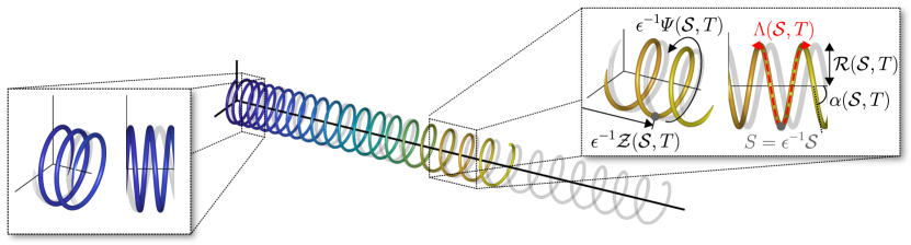
Figure 2: Multiple-scales analysis of highly-coiled helical filaments with a straight helix axis, presented using dimensionless quantities (lengths scaled by the undeformed contour wavelength, $\lambda^{u}$). Each close-up shows a helical wave centred around the point with ‘slow’ variable $\mathcal{S}$ (where $s=\epsilon^{-1}\lambda^{u}\mathcal{S}$), together with the undeformed filament (grey curve). The deformed shape is locally another helix with pitch angle $\alpha$ and dimensionless wavelength $\Lambda=\lambda/\lambda^{u}$, where $\alpha$ and $\Lambda$ vary with $\mathcal{S}$. Because the filament tip is free of forces and moments, $\alpha\approx\alpha^{u}$ and $\Lambda\approx 1$ in its vicinity and the shape resembles a translation of the undeformed helix (right close-up). Elsewhere, the helical parameters may deviate significantly (left close-up).

Recall that we assume that the deformation is principally driven by the external force, and that the filament tip is free of forces and moments. Integrating Eq. (18) backwards from the tip shows that the force resultant at arclength $S$ is of magnitude $|\mathbf{F}(S,T)|=\operatorname{ord}(\epsilon(L-S))$. We will show below that the dimensionless force resultant is of the same order as the change in helical parameters from their undeformed values, i.e. $(\alpha-\alpha^{u})$ and $(\Lambda-1)$. We therefore have

$$\left\lvert\alpha(\mathcal{S},T)-\alpha^{u}\right\rvert=O(\epsilon(L-S)),\quad\left\lvert\Lambda(\mathcal{S},T)-1\right\rvert=O(\epsilon(L-S)).$$ (24)

The slow lengthscale $\mathcal{S}$, over which the helical geometry varies significantly, is then defined by

$$S=\epsilon^{-1}\mathcal{S}.$$ (25)

In what follows we consider $\epsilon L=O(1)$, so that $\mathcal{S}=O(1)$ throughout the filament and hence $O(1)$ changes to the helical geometry may occur.

We also assume that any unsteadiness in the deformation is driven by the external force. Balancing the inertia term on the right-hand side of Eq. (18) with the external force, and using the scaling behaviour $|\mathbf{R}|=O(L)=O(\epsilon^{-1})$, we obtain $t^{*}/[t]=O(\epsilon)$. Hence, we choose the timescale

$$[t]=\epsilon^{-1}t^{*}.$$ (26)

The basis of the multiple-scales method is to formally treat $S$ and $\mathcal{S}$ as independent variables. The chain rule then implies that

$$\frac{\partial}{\partial S}=\frac{\partial}{\partial S}\bigg{\lvert}_{\mathcal{S}}+\epsilon\frac{\partial}{\partial\mathcal{S}}\bigg{\lvert}_{S}.$$ (27)

Throughout the following analysis, we consider $S$ varying over a general helical wave centred around the point with slow variable $\mathcal{S}$, i.e., $S=\epsilon^{-1}\mathcal{S}+\Delta S$ where $\Delta S\in(-\Lambda/2,\Lambda/2)$; see Fig. 2. Later, we will integrate the force and moment balances with respect to $S$ over each wavelength, leading to evolution equations as $\mathcal{S}$ and $T$ vary.

3.2 Locally-helical kinematics

Before proceeding, we derive the kinematic quantities associated with our ansatz of a locally-helical shape. Let $\{\mathbf{n},\mathbf{b},\mathbf{t}\}$ be the Frenet-Serret frame at the helical wave centred at $\mathcal{S}$, associated with the local values of the pitch angle $\alpha$ and contour wavelength $\Lambda$. By analogy with the Frenet-Serret frame associated with the undeformed centreline, Eq. (5) (see also Fig. 1b), we postulate that

$$\mathbf{n}(S,\mathcal{S},T) =-\mathbf{e}_{r}(S,\mathcal{S},T),$$

$$\mathbf{b}(S,\mathcal{S},T) =-\cos\alpha(\mathcal{S},T)\,\mathbf{e}_{\theta}(S,\mathcal{S},T)+h\sin\alpha(\mathcal{S},T)\,\mathbf{e}_{z},$$

$$\mathbf{t}(S,\mathcal{S},T) =h\sin\alpha(\mathcal{S},T)\,\mathbf{e}_{\theta}(S,\mathcal{S},T)+\cos\alpha(\mathcal{S},T)\,\mathbf{e}_{z},$$ (28)

where $\mathbf{e}_{r}(S,\mathcal{S},T)$ and $\mathbf{e}_{\theta}(S,\mathcal{S},T)$ are the radial and azimuthal unit vectors, respectively, evaluated on the centreline. (Here we are assuming that there is no change in chirality of the helix from its undeformed value, $h$.) These unit vectors are now parameterised by the unknown winding angle $\Psi(S,\mathcal{S},T)$ of the deformed helix:

$$\mathbf{e}_{r}(S,\mathcal{S},T)=\cos\Psi(S,\mathcal{S},T)\,\mathbf{e}_{x}+\sin\Psi(S,\mathcal{S},T)\,\mathbf{e}_{y},\quad\mathbf{e}_{\theta}(S,\mathcal{S},T)=-\sin\Psi(S,\mathcal{S},T)\,\mathbf{e}_{x}+\cos\Psi(S,\mathcal{S},T)\,\mathbf{e}_{y}.$$ (29)

Because the local contour wavelength is $\Lambda$, we have

$$\frac{\partial\Psi}{\partial S}\bigg{\lvert}_{\mathcal{S}}=\frac{2\pi h}{\Lambda}.$$ (30)

After integrating, note that in general $\Psi\neq 2\pi hS/\Lambda$, i.e., the additive function of $\mathcal{S}$ is generally non-zero. We will show below that this corresponds to a slowly-varying phase shift that accounts for the variation in $\Lambda$ up to the wavelength centred at $\mathcal{S}$.

We write $\{\mathbf{d}_{1}^{(0)},\mathbf{d}_{2}^{(0)},\mathbf{d}_{3}^{(0)}\}$ for the leading-order directors associated with the locally-helical shape. Because we assume that the rod is unshearable, $\mathbf{d}_{3}^{(0)}$ coincides with the unit tangent vector: $\mathbf{d}_{3}^{(0)}=\mathbf{t}$. The other directors $\{\mathbf{d}_{1}^{(0)},\mathbf{d}_{2}^{(0)}\}$ are then a rotation of the Frenet-Serret basis vectors $\{\mathbf{n},\mathbf{b}\}$ according to the excess axial twist. However, we note that the force balance (18) and moment balance (21) are both homogeneous at leading order in $\epsilon$ (using $[t]=\epsilon^{-1}t^{*}$ and $\delta=O(1)$). For a stationary helical rod in the absence of distributed loads, it can be shown that the excess twist must equal its undeformed value, in this case zero (Goriely and Tabor, 1997c). As a consequence, the leading-order directors are precisely the Frenet-Serret basis vectors reported above (Eq. (28)):

$$\mathbf{d}_{1}^{(0)}=\mathbf{n},\quad\mathbf{d}_{2}^{(0)}=\mathbf{b},\quad\mathbf{d}_{3}^{(0)}=\mathbf{t}.$$ (31)

We can determine the leading-order centreline, denoted $\mathbf{R}^{(0)}$, and winding angle, $\Psi$, by solving the inextensibility constraint (14) with the tangent vector $\mathbf{d}_{3}^{(0)}$ above. The calculation, detailed in AppendixA, yields

$$\mathbf{R}^{(0)}(S,\mathcal{S},T) =\mathcal{R}(\mathcal{S},T)\,\mathbf{e}_{r}(S,\mathcal{S},T)+\left[\epsilon^{-1}\mathcal{Z}(\mathcal{S},T)+\Delta S\cos\alpha(\mathcal{S},T)\right]\mathbf{e}_{z},$$ (32)

$$\Psi(S,\mathcal{S},T) =\epsilon^{-1}\varPsi(\mathcal{S},T)+\frac{2\pi h\Delta S}{\Lambda(\mathcal{S},T)},$$ (33)

where $\mathcal{R}(\mathcal{S},T)$ is the slowly-varying helical radius, $\mathcal{Z}(\mathcal{S},T)$ is the wavelength-averaged longitudinal coordinate, and $\varPsi(\mathcal{S},T)$ is the wavelength-averaged winding angle (see Fig. 2). In terms of the slowly-varying pitch angle $\alpha$ and wavelength $\Lambda$, these are given by (AppendixA)

$$\mathcal{R}(\mathcal{S},T)=\frac{\Lambda(\mathcal{S},T)\sin\alpha(\mathcal{S},T)}{2\pi},\quad\mathcal{Z}(\mathcal{S},T)=\int_{0}^{\mathcal{S}}\cos\alpha(\xi,T)\,\mathrm{d}\xi,\quad\varPsi(\mathcal{S},T)=2\pi h\int_{0}^{\mathcal{S}}\frac{\mathrm{d}\xi}{\Lambda(\xi,T)},$$ (34)

where we have made use of the boundary condition at the filament base, Eq. (23). These expressions show how changes to $\alpha$ and $\Lambda$ correspond to extensional (longitudinal) and torsional deformations about the helix axis.

If the external force and moment are known functions of the position and orientation of the rod, i.e., $\mathbf{M}_{e}=\mathbf{M}_{e}(\mathbf{R},\mathbf{d}_{i})$ and $\mathbf{F}_{e}=\mathbf{F}_{e}(\mathbf{R},\mathbf{d}_{i})$, formally we can expand

$$\mathbf{M}_{e}\sim\mathbf{M}_{e}^{(0)},\quad\mathbf{F}_{e}\sim\mathbf{F}_{e}^{(0)}\qquad\mathrm{where}\qquad\mathbf{M}_{e}^{(0)}\equiv\mathbf{M}_{e}\left(\mathbf{R}^{(0)},\mathbf{d}_{i}^{(0)}\right),\quad\mathbf{F}_{e}^{(0)}\equiv\mathbf{F}_{e}\left(\mathbf{R}^{(0)},\mathbf{d}_{i}^{(0)}\right).$$

Equations (31)–(34) can then be used to express the external loads in terms of the slowly-varying parameters $\alpha$ and $\Lambda$. For later reference, we also calculate the centreline velocity and acceleration using the above expression for $\mathbf{R}^{(0)}$:

$$\frac{\partial\mathbf{R}^{(0)}}{\partial T} =\frac{\partial\mathcal{R}}{\partial T}\mathbf{e}_{r}+\mathcal{R}\left(\epsilon^{-1}\frac{\partial\varPsi}{\partial T}-\frac{2\pi h\Delta S}{\Lambda^{2}}\frac{\partial\Lambda}{\partial T}\right)\mathbf{e}_{\theta}+\left(\epsilon^{-1}\frac{\partial\mathcal{Z}}{\partial T}-\Delta S\frac{\partial\alpha}{\partial T}\sin\alpha\right)\mathbf{e}_{z}$$

$$=\epsilon^{-1}\left(\mathcal{R}\frac{\partial\varPsi}{\partial T}\mathbf{e}_{\theta}+\frac{\partial\mathcal{Z}}{\partial T}\mathbf{e}_{z}\right)+O(1),$$ (35)

$$\frac{\partial^{2}\mathbf{R}^{(0)}}{\partial T^{2}} =-\epsilon^{-2}\mathcal{R}\left(\frac{\partial\varPsi}{\partial T}\right)^{2}\mathbf{e}_{r}+\epsilon^{-1}\left[\frac{4\pi h\Delta S}{\Lambda^{2}}\frac{\partial\Lambda}{\partial T}\frac{\partial\varPsi}{\partial T}\mathcal{R}\mathbf{e}_{r}+\frac{1}{\mathcal{R}}\frac{\partial}{\partial T}\left(\mathcal{R}^{2}\frac{\partial\varPsi}{\partial T}\right)\mathbf{e}_{\theta}+\frac{\partial^{2}\mathcal{Z}}{\partial T^{2}}\mathbf{e}_{z}\right]+O(1).$$ (36)

3.3 Perturbation scheme

Following Goriely and Tabor (1997a, b), we choose to not express the rod equations in component form with respect to a fixed external basis (using, for example, Euler angles to parameterise the directors) before perturbing quantities. Instead, we seek a regular perturbation expansion of the directors themselves in powers of $\epsilon$:

$$\mathbf{d}_{i}=\mathbf{d}_{i}^{(0)}+\epsilon\,\mathbf{d}_{i}^{(1)}+O(\epsilon^{2}),\qquad i=1,2,3.$$

We need to ensure that the director basis remains orthonormal at each order of the expansion, i.e.

$$\delta_{ij}=\mathbf{d}_{i}\cdot\mathbf{d}_{j}=\mathbf{d}_{i}^{(0)}\cdot\mathbf{d}_{j}^{(0)}+\epsilon\left[\mathbf{d}_{i}^{(0)}\cdot\mathbf{d}_{j}^{(1)}+\mathbf{d}_{i}^{(1)}\cdot\mathbf{d}_{j}^{(0)}\right]+O(\epsilon^{2}),$$

where $\delta_{ij}$ is the Kronecker delta. As explained by previous authors (Goriely and Tabor, 1997a; Katsamba and Lauga, 2019), the $O(\epsilon)$ term in the above equation vanishes for all $i,j\in\{1,2,3\}$ if and only if there exists a vector $\boldsymbol{\Phi}$ such that

$$\mathbf{d}_{i}^{(1)}=\boldsymbol{\Phi}\times\mathbf{d}_{i}^{(0)},\qquad i=1,2,3.$$ (37)

In addition, we expand the components (in the director basis) of the strain vector $\mathbf{U}$, angular velocity vector $\boldsymbol{\Omega}$, resultant force $\mathbf{F}$ and resultant moment $\mathbf{M}$ in powers of $\epsilon$:

$$U_{i}=U_{i}^{(0)}+\epsilon\,U_{i}^{(1)}+O(\epsilon^{2}),\quad\Omega_{i}=\Omega_{i}^{(0)}+\epsilon\,\Omega_{i}^{(1)}+O(\epsilon^{2}),\quad M_{i}=M_{i}^{(0)}+\epsilon\,M_{i}^{(1)}+O(\epsilon^{2}),\quad F_{i}=F_{i}^{(0)}+\epsilon\,F_{i}^{(1)}+O(\epsilon^{2}).$$ (38)

The advantage of this approach is that we can readily obtain the expansions of the vectors $\mathbf{U}$, $\boldsymbol{\Omega}$, $\mathbf{F}$ and $\mathbf{M}$ using Eqs. (37)–(38). Explicitly, for a general vector $\mathbf{W}=\sum_{i}W_{i}\mathbf{d}_{i}$ whose components have the regular expansion $W_{i}=W_{i}^{(0)}+\epsilon\,W_{i}^{(1)}+O(\epsilon^{2})$, we note that $\mathbf{W}$ has the expansion (Goriely and Tabor, 1997a)

$$\mathbf{W}=\sum_{i=1}^{3}W_{i}\mathbf{d}_{i}=\mathbf{W}^{(0)}+\epsilon\,\mathbf{W}^{(1)}+O(\epsilon^{2})\qquad\mathrm{where}\qquad\mathbf{W}^{(0)}=\sum_{i=1}^{3}W_{i}^{(0)}\mathbf{d}_{i}^{(0)},\quad\mathbf{W}^{(1)}=\sum_{i=1}^{3}W_{i}^{(1)}\mathbf{d}_{i}^{(0)}+\boldsymbol{\Phi}\times\mathbf{W}^{(0)}.$$ (39)

In what follows, we will use this identity with $\mathbf{W}=\mathbf{U}$, $\boldsymbol{\Omega}$, $\mathbf{M}$ and $\mathbf{F}$. Our method is to substitute the above expansions into the dimensionless equations derived in §2.4, expand spatial derivatives using the chain rule in (27), and solve at each successive order in $\epsilon$.

3.4 Leading-order problem

The kinematic equations (15) at leading order are

$$\frac{\partial\mathbf{d}_{i}^{(0)}}{\partial S}\bigg{\lvert}_{\mathcal{S}}=\mathbf{U}^{(0)}\times\mathbf{d}_{i}^{(0)},\quad\frac{\partial\mathbf{d}_{i}^{(0)}}{\partial T}=\boldsymbol{\Omega}^{(0)}\times\mathbf{d}_{i}^{(0)},\qquad i=1,2,3.$$ (40)

Substituting the ansatz (31) for the leading-order directors $\mathbf{d}_{i}^{(0)}$, and evaluating derivatives of the Frenet-Serret basis vectors $\{\mathbf{n},\mathbf{b},\mathbf{t}\}$ using Eqs. (28)–(30), we obtain

$$\mathbf{U}^{(0)}=\mathcal{K}\mathbf{b}+\mathcal{T}\mathbf{t}=\frac{2\pi h}{\Lambda}\mathbf{e}_{z},\quad\boldsymbol{\Omega}^{(0)}=h\frac{\partial\alpha}{\partial T}\mathbf{n}+\frac{\partial\Psi}{\partial T}\mathbf{e}_{z},$$ (41)

i.e., $\mathbf{U}^{(0)}$ is simply the Darboux vector associated with the Frenet-Serret frame $\{\mathbf{n},\mathbf{b},\mathbf{t}\}$, where the slowly-varying Frenet curvature $\mathcal{K}(\mathcal{S},T)$ and torsion $\mathcal{T}(\mathcal{S},T)$ are

$$\mathcal{K}(\mathcal{S},T)=\frac{2\pi\sin\alpha(\mathcal{S},T)}{\Lambda(\mathcal{S},T)},\quad\mathcal{T}(\mathcal{S},T)=\frac{2\pi h\cos\alpha(\mathcal{S},T)}{\Lambda(\mathcal{S},T)}.$$ (42)

When the filament is undeformed, we have $\mathcal{K}=\mathcal{K}^{u}$, $\mathcal{T}=\mathcal{T}^{u}$, and $\{\mathbf{n},\mathbf{b},\mathbf{t}\}=\{\mathbf{n}^{u},\mathbf{b}^{u},\mathbf{t}^{u}\}$; the expression for $\mathbf{U}^{(0)}$ then coincides with the undeformed strain vector, $\mathbf{U}^{u}=\mathcal{K}^{u}\mathbf{b}^{u}+\mathcal{T}^{u}\mathbf{t}^{u}$, given earlier in Eq. (17).

The force balance (18) and moment balance (21) at leading-order are

$$\frac{\partial\mathbf{F}^{(0)}}{\partial S}\bigg{\lvert}_{\mathcal{S}}=\mathbf{0},$$ (43)

$$\frac{\partial\mathbf{M}^{(0)}}{\partial S}\bigg{\lvert}_{\mathcal{S}}+\mathbf{d}_{3}^{(0)}\times\mathbf{F}^{(0)}=\mathbf{0}.$$ (44)

The constitutive law (22) with $\mathbf{U}^{(0)}$ above (Eq. (41)) gives

$$M_{1}^{(0)}=0,\quad M_{2}^{(0)}=\mathcal{K}-\mathcal{K}^{u},\quad M_{3}^{(0)}=\frac{\mathcal{T}-\mathcal{T}^{u}}{1+\nu}.$$ (45)

The force resultant satisfying Eqs. (43)–(44) is then (Goriely and Tabor, 1997c)

$$\mathbf{F}^{(0)}=\left(\frac{\mathcal{T}-\mathcal{T}^{u}}{1+\nu}-\mathcal{T}\frac{\mathcal{K}-\mathcal{K}^{u}}{\mathcal{K}}\right)\mathbf{U}^{(0)}.$$ (46)

To see that $\mathbf{F}^{(0)}$ is indeed independent of $S$, as required by Eq. (43), we note from Eq. (41) that $\mathbf{U}^{(0)}=(2\pi h/\Lambda)\mathbf{e}_{z}$. We delay discussing the boundary conditions at the filament tip, Eq. (23), until §3.6.

For later reference, we also write the resultants in terms of the unit vectors in cylindrical polar coordinates. Making use of Eqs. (28) and (42), we obtain

$$\mathbf{M}^{(0)}=\mathcal{R}F_{Z}\mathbf{e}_{\theta}+M_{Z}\mathbf{e}_{z},\quad\mathbf{F}^{(0)}=F_{Z}\mathbf{e}_{z},$$ (47)

where the slowly-varying radius $\mathcal{R}$ was defined in Eq. (34), and $M_{Z}(\mathcal{S},T)$ and $F_{Z}(\mathcal{S},T)$ are given by

$$M_{Z}=\frac{\Lambda}{2\pi h}\left[\mathcal{K}\left(\mathcal{K}-\mathcal{K}^{u}\right)+\mathcal{T}\frac{\mathcal{T}-\mathcal{T}^{u}}{1+\nu}\right],\quad F_{Z}=\frac{2\pi h}{\Lambda}\left(\frac{\mathcal{T}-\mathcal{T}^{u}}{1+\nu}-\mathcal{T}\frac{\mathcal{K}-\mathcal{K}^{u}}{\mathcal{K}}\right).$$ (48)

We see that the moment resultant is composed of two terms: part of a wrench associated with torsion/winding about the helix axis ($Z$-axis), and a torque produced by the force resultant equal to $-\mathcal{R}\mathbf{e}_{r}\times\mathbf{F}^{(0)}$. This second term arises because the force resultant $\mathbf{F}^{(0)}$ is applied at the rod centreline, a distance $\mathcal{R}$ from the helix axis.

We remark that an alternative method of solving the leading-order problem, which does not require posing the ansatz of a locally-helical shape a priori, is to solve the homogeneous force and moment balances (43)–(44) directly. The general solution is a linear combination of six solutions whose coefficients depend on the slow variable, $\mathcal{S}$. Two of these solutions correspond to a space-curve with slowly-varying Frenet curvature and torsion, and so yield a locally-helical solution; the other solutions correspond to bending about the $X$ and $Y$-axes, and so must vanish if the helix axis remains straight. Thus, the locally-helical form of the solution follows from the assumption of a straight helical axis. The disadvantage of this approach is that the interpretation of the slowly-varying coefficients in terms of physical parameters of the helix shape (e.g. pitch angle and wavelength) is less clear than simply seeking a locally-helical solution to begin with.

3.5 First-order problem

3.5.1 Derivation of equations

At $O(\epsilon)$, the kinematic equations (15) for the strain vector become

$$\frac{\partial\mathbf{d}_{i}^{(1)}}{\partial S}\bigg{\lvert}_{\mathcal{S}}+\frac{\partial\mathbf{d}_{i}^{(0)}}{\partial\mathcal{S}}\bigg{\lvert}_{S}=\mathbf{U}^{(0)}\times\mathbf{d}_{i}^{(1)}+\mathbf{U}^{(1)}\times\mathbf{d}_{i}^{(0)},\qquad i=1,2,3.$$

As well as $\mathcal{S}$-derivatives now appearing, the vectors at this order contain both perturbations to the components (in the director basis) and perturbations to the directors; recall the identity (39). In particular, substituting $\mathbf{d}_{i}^{(1)}=\boldsymbol{\Phi}\times\mathbf{d}_{i}^{(0)}$ and the expression for $\mathbf{U}^{(1)}$ (from setting $\mathbf{W}=\mathbf{U}$ in (39)), and making use of the leading-order kinematic equations (40), the above simplifies to

$$\frac{\partial\boldsymbol{\Phi}}{\partial S}\bigg{\lvert}_{\mathcal{S}}\times\mathbf{d}_{i}^{(0)}+\frac{\partial\mathbf{d}_{i}^{(0)}}{\partial\mathcal{S}}\bigg{\lvert}_{S}=\left(\sum_{j=1}^{3}U_{j}^{(1)}\mathbf{d}_{j}^{(0)}\right)\times\mathbf{d}_{i}^{(0)},\qquad i=1,2,3.$$ (49)

We note from Eqs. (28)–(31) that the leading-order directors $\mathbf{d}_{i}^{(0)}$ depend on the slow variable $\mathcal{S}$ and time $T$ only via the pitch angle $\alpha(\mathcal{S},T)$ and wavelength $\Lambda(\mathcal{S},T)$. Hence, $\mathcal{S}$-derivatives of $\mathbf{d}_{i}^{(0)}$ can be calculated analogously to time derivatives. By analogy with Eqs. (40)–(41), we find that

$$\frac{\partial\mathbf{d}_{i}^{(0)}}{\partial\mathcal{S}}\bigg{\lvert}_{S}=\boldsymbol{\Theta}\times\mathbf{d}_{i}^{(0)}\qquad\mathrm{where}\qquad\boldsymbol{\Theta}\equiv h\frac{\partial\alpha}{\partial\mathcal{S}}\bigg{\lvert}_{S}\mathbf{n}+\frac{\partial\Psi}{\partial\mathcal{S}}\bigg{\lvert}_{S}\mathbf{e}_{z}.$$ (50)

Substituting into Eq. (49), and noting that $(\cdot)\times\mathbf{d}_{i}^{(0)}=\mathbf{0}$ for $i=1,2,3$ implies that $(\cdot)=\mathbf{0}$, we obtain

$$\frac{\partial\boldsymbol{\Phi}}{\partial S}\bigg{\lvert}_{\mathcal{S}}-\sum_{j=1}^{3}U_{j}^{(1)}\mathbf{d}_{j}^{(0)}+\boldsymbol{\Theta}=\mathbf{0}.$$ (51)

Without the $\boldsymbol{\Theta}$-term, this is analogous to Eq. (51) in Goriely and Tabor (1997a) and Eq. (27) in Katsamba and Lauga (2019). The $\boldsymbol{\Theta}$-term enters here because we are considering slow changes in the (currently unknown) leading-order shape, in addition to localised perturbations to the leading-order shape. From the scaling estimates (24), we have that $\left\lvert\alpha-\alpha^{u}\right\rvert=O(\epsilon L)$ and $\left\lvert\Lambda-1\right\rvert=O(\epsilon L)$ at the filament base, and hence $\boldsymbol{\Theta}=O(\epsilon L)$ from Eq. (50). It follows that the $\boldsymbol{\Theta}$-term can be neglected if $\epsilon L\ll 1$ (corresponding to small deformations away from the undeformed shape), but must be considered in the general case $\epsilon L=O(1)$.

With $\delta=O(1)$ and $[t]=\epsilon^{-1}t^{*}$ (recall Eq. (26)), the force balance (18) and moment balance (21) at $O(\epsilon)$ are

$$\frac{\partial\mathbf{F}^{(1)}}{\partial S}\bigg{\lvert}_{\mathcal{S}}=-\frac{\partial\mathbf{F}^{(0)}}{\partial\mathcal{S}}\bigg{\lvert}_{S}-\mathbf{F}_{e}^{(0)}+\epsilon\frac{\partial^{2}\mathbf{R}^{(0)}}{\partial T^{2}},$$ (52)

$$\frac{\partial\mathbf{M}^{(1)}}{\partial S}\bigg{\lvert}_{\mathcal{S}}+\mathbf{d}_{3}^{(0)}\times\mathbf{F}^{(1)}+\mathbf{d}_{3}^{(1)}\times\mathbf{F}^{(0)}=-\frac{\partial\mathbf{M}^{(0)}}{\partial\mathcal{S}}\bigg{\lvert}_{S}-\delta\mathbf{M}_{e}^{(0)}.$$ (53)

Equations (52)–(53) are linear in the first-order resultants $\mathbf{F}^{(1)}$ and $\mathbf{M}^{(1)}$; the inhomogeneous terms on the right-hand sides arise from inertia, external forces/moments and slow derivatives of the leading-order resultants. Note that, without the $\mathbf{d}_{3}^{(1)}\times\mathbf{F}^{(0)}$ term in (53), the differential operator applied to $(\mathbf{F}^{(1)},\mathbf{M}^{(1)})$ is identical to that in the leading-order problem, i.e., Eqs. (43)–(44). The $\mathbf{d}_{3}^{(1)}\times\mathbf{F}^{(0)}$ term accounts for the correction to the moment produced by $\mathbf{F}^{(0)}$ due to the perturbation $\mathbf{d}_{3}^{(1)}$ to the tangent vector, and may only be neglected if $\epsilon L\ll 1$, similar to the $\boldsymbol{\Theta}$-term above.

We insert the expressions for $\mathbf{F}^{(1)}$ and $\mathbf{M}^{(1)}$ (from setting $\mathbf{W}=\mathbf{F}$, $\mathbf{M}$ in Eq. (39)) into Eqs. (52)–(53) and evaluate derivatives of $\mathbf{d}_{i}^{(0)}$, $\mathbf{F}^{(0)}$ and $\mathbf{M}^{(0)}$ using the leading-order equations (40) and (43)–(44). After eliminating $\boldsymbol{\Phi}$ derivatives using Eq. (51), and expanding the $\mathcal{S}$-derivatives of $\mathbf{F}^{(0)}$ and $\mathbf{M}^{(0)}$ using Eq. (50), the terms in $\boldsymbol{\Phi}$ and $\boldsymbol{\Theta}$ cancel yielding

$$\sum_{i=1}^{3}\frac{\partial F_{i}^{(1)}}{\partial S}\bigg{\lvert}_{\mathcal{S}}\mathbf{d}_{i}^{(0)}+\mathbf{U}^{(0)}\times\left(\sum_{i=1}^{3}F_{i}^{(1)}\mathbf{d}_{i}^{(0)}\right)+\left(\sum_{i=1}^{3}U_{i}^{(1)}\mathbf{d}_{i}^{(0)}\right)\times\mathbf{F}^{(0)}=-\sum_{i=1}^{3}\frac{\partial F_{i}^{(0)}}{\partial\mathcal{S}}\bigg{\lvert}_{S}\mathbf{d}_{i}^{(0)}-\mathbf{F}_{e}^{(0)}+\epsilon\frac{\partial^{2}\mathbf{R}^{(0)}}{\partial T^{2}},$$ (54)

$$\sum_{i=1}^{3}\frac{\partial M_{i}^{(1)}}{\partial S}\bigg{\lvert}_{\mathcal{S}}\mathbf{d}_{i}^{(0)}+\mathbf{U}^{(0)}\times\left(\sum_{i=1}^{3}M_{i}^{(1)}\mathbf{d}_{i}^{(0)}\right)+\left(\sum_{i=1}^{3}U_{i}^{(1)}\mathbf{d}_{i}^{(0)}\right)\times\mathbf{M}^{(0)}+\mathbf{d}_{3}^{(0)}\times\left(\sum_{i=1}^{3}F_{i}^{(1)}\mathbf{d}_{i}^{(0)}\right)=-\sum_{i=1}^{3}\frac{\partial M_{i}^{(0)}}{\partial\mathcal{S}}\bigg{\lvert}_{S}\mathbf{d}_{i}^{(0)}-\delta\mathbf{M}_{e}^{(0)}.$$ (55)

Finally, the constitutive law (22) gives

$$M_{1}^{(1)}=U_{1}^{(1)},\quad M_{2}^{(1)}=U_{2}^{(1)},\quad M_{3}^{(1)}=\frac{U_{3}^{(1)}}{1+\nu}.$$ (56)

Equations (51) and (54)–(56) provide a closed system of equations for which solvability conditions can be formulated.

3.5.2 Periodicity and solvability

For general $\epsilon L=O(1)$, it can be shown that the homogeneous problem at first order, consisting of the homogeneous versions of Eqs. (51) and (54)–(56), has non-trivial solutions. From the Fredholm Alternative Theorem (Keener, 1988), solutions to the inhomogeneous problem then exist only if the inhomogeneous terms satisfy certain solvability conditions. These solvability conditions take the form of partial differential equations (PDEs) for the slowly-varying helix geometry.

To formulate the solvability conditions, we assume that the first-order components — namely $U_{i}^{(1)}$, $F_{i}^{(1)}$, $M_{i}^{(1)}$ and the components of $\boldsymbol{\Phi}$ — are locally periodic over the helical wave centred at $S=\epsilon^{-1}\mathcal{S}$ (i.e., they are $\Lambda$-periodic). With this assumption, two approaches are then possible. In the first approach, we directly average the first-order equations over the helical wavelength $S\in(\epsilon^{-1}\mathcal{S}-\Lambda/2,\epsilon^{-1}\mathcal{S}+\Lambda/2)$, exploiting periodicity of the first-order components to eliminate all unknown variables so that only the leading-order components $F_{i}^{(0)}$ , $M_{i}^{(0)}$ and the terms $\partial^{2}\mathbf{R}^{(0)}/\partial T^{2}$, $\mathbf{F}_{e}^{(0)}$ and $\mathbf{M}_{e}^{(0)}$ remain. The resulting equations can then be written as a closed system for $\alpha$ and $\Lambda$.

In the second approach, we write the first-order equations as a linear system of equations for the nine-dimensional vector $\mathbf{Y}^{(1)}=\{\boldsymbol{\Phi},F_{1}^{(1)},F_{2}^{(1)},F_{3}^{(1)},M_{1}^{(1)},M_{2}^{(1)},M_{3}^{(1)}\}$ (using Eq. (56) to eliminate $U_{i}^{(1)}$ in terms of $M_{i}^{(1)}$). The Fredholm Alternative Theorem states that the inhomogeneous part of this linear system must be orthogonal to $\Lambda$-periodic solutions of the homogeneous adjoint problem, when multiplied and integrated over the helical wavelength. This is a necessary condition for the first-order solution to be locally periodic and hence bounded across the filament, and is analogous to removing secular terms in the classical Poincaré-Lindstedt method. The leading-order solution should then provide a uniformly valid approximation of the filament shape (Goriely et al., 2001).

Below, we present the direct approach since it readily yields the correct solvability conditions and makes their physical significance clear. Nevertheless, as this method is somewhat ad hoc, in AppendixB we show that the same conditions can be derived systematically using the second approach via the Fredholm Alternative Theorem.

3.5.3 Solvability conditions: direct approach

From the periodicity of $F_{i}^{(1)}$ and $M_{i}^{(1)}$, it follows that

$$\overline{\frac{\partial F_{i}^{(1)}}{\partial S}\bigg{\lvert}_{\mathcal{S}}}=0,\quad\overline{\frac{\partial M_{i}^{(1)}}{\partial S}\bigg{\lvert}_{\mathcal{S}}}=0,$$

where we use bars to denote the average over the helical wave centred at $S=\epsilon^{-1}\mathcal{S}$, i.e., for a function $f(S,\mathcal{S},T)$,

$$\overline{f}(\mathcal{S},T)\equiv\frac{1}{\Lambda}\int_{\epsilon^{-1}\mathcal{S}-\Lambda/2}^{\epsilon^{-1}\mathcal{S}+\Lambda/2}f(S,\mathcal{S},T)\>\mathrm{d}S.$$

From Eqs. (28) and (31), the leading-order directors $\mathbf{d}_{i}^{(0)}$ depend on the fast variable $S$ only via the unit vectors $\mathbf{e}_{r}$ and $\mathbf{e}_{\theta}$; the coefficients of $\mathbf{e}_{r}$, $\mathbf{e}_{\theta}$ and $\mathbf{e}_{z}$ depend only on the slow variable, $\mathcal{S}$. Hence,

$$\overline{\mathbf{e}_{r}\cdot\left(\sum_{i=1}^{3}\frac{\partial F_{i}^{(1)}}{\partial S}\bigg{\lvert}_{\mathcal{S}}\mathbf{d}_{i}^{(0)}\right)}=0,\quad\overline{\mathbf{e}_{\theta}\cdot\left(\sum_{i=1}^{3}\frac{\partial F_{i}^{(1)}}{\partial S}\bigg{\lvert}_{\mathcal{S}}\mathbf{d}_{i}^{(0)}\right)}=0,\quad\overline{\mathbf{e}_{z}\cdot\left(\sum_{i=1}^{3}\frac{\partial F_{i}^{(1)}}{\partial S}\bigg{\lvert}_{\mathcal{S}}\mathbf{d}_{i}^{(0)}\right)}=0.$$ (57)

Identical expressions hold with $F_{i}^{(1)}$ replaced by $M_{i}^{(1)}$.

Dotting Eq. (54) by $\mathbf{e}_{z}$ and averaging over the helical wave, all unknown terms on the left-hand side vanish according to Eq. (57) and the fact that $\mathbf{U}^{(0)}$ and $\mathbf{F}^{(0)}$ are both parallel to $\mathbf{e}_{z}$ (recall Eqs. (41) and (47)). We are left with the solvability condition

$$0=-\overline{\mathbf{e}_{z}\cdot\left(\sum_{i=1}^{3}\frac{\partial F_{i}^{(0)}}{\partial\mathcal{S}}\bigg{\lvert}_{S}\mathbf{d}_{i}^{(0)}\right)}-\overline{\mathbf{e}_{z}\cdot\mathbf{F}_{e}^{(0)}}+\overline{\mathbf{e}_{z}\cdot\epsilon\frac{\partial^{2}\mathbf{R}^{(0)}}{\partial T^{2}}}.$$ (58)

If we instead dot Eq. (54) by $\mathcal{R}\mathbf{e}_{\theta}$, dot Eq. (55) by $\mathbf{e}_{z}$ and add the resulting equations, the terms in $F_{i}^{(1)}$ and $U_{i}^{(1)}$ cancel. Averaging over the helical wave and making use of Eq. (57), all remaining terms on the left-hand side again vanish, yielding

$$0=-\mathcal{R}\overline{\mathbf{e}_{\theta}\cdot\left(\sum_{i=1}^{3}\frac{\partial F_{i}^{(0)}}{\partial\mathcal{S}}\bigg{\lvert}_{S}\mathbf{d}_{i}^{(0)}\right)}-\mathcal{R}\overline{\mathbf{e}_{\theta}\cdot\mathbf{F}_{e}^{(0)}}+\mathcal{R}\overline{\mathbf{e}_{\theta}\cdot\epsilon\frac{\partial^{2}\mathbf{R}^{(0)}}{\partial T^{2}}}-\overline{\mathbf{e}_{z}\cdot\left(\sum_{i=1}^{3}\frac{\partial M_{i}^{(0)}}{\partial\mathcal{S}}\bigg{\lvert}_{S}\mathbf{d}_{i}^{(0)}\right)}-\delta\overline{\mathbf{e}_{z}\cdot\mathbf{M}_{e}^{(0)}}.$$ (59)

These first two solvability conditions can be interpreted as wavelength-averaged force and moment balances, respectively, about the helix axis.

The remaining solvability conditions can be formulated by noting from the definition of $\boldsymbol{\Theta}$ (Eq. (50)) that $\overline{\mathbf{e}_{x}\cdot\boldsymbol{\Theta}}=0$ and $\overline{\mathbf{e}_{y}\cdot\boldsymbol{\Theta}}=0$. Because the components of $\boldsymbol{\Phi}$ are assumed to be $\Lambda$-periodic, we also have $\overline{\partial\boldsymbol{\Phi}/\partial S\lvert_{\mathcal{S}}}=\mathbf{0}$ (since the $\mathbf{d}_{i}^{(0)}$ are also periodic). Equation (51) then gives

$$\overline{\mathbf{e}_{x}\cdot\left(\sum_{i=1}^{3}U_{i}^{(1)}\mathbf{d}_{i}^{(0)}\right)}=0,\quad\overline{\mathbf{e}_{y}\cdot\left(\sum_{i=1}^{3}U_{i}^{(1)}\mathbf{d}_{i}^{(0)}\right)}=0.$$ (60)

We dot (54) in turn by $\mathbf{e}_{x}$ and $\mathbf{e}_{y}$ and average over the helical wave. The first two terms in (54) can be written as the single derivative $\partial(\sum_{i=1}^{3}F_{i}^{(1)}\mathbf{d}_{i}^{(0)})/\partial S\lvert_{\mathcal{S}}$; since $\mathbf{e}_{x}$ and $\mathbf{e}_{y}$ are constant vectors, this derivative (after taking the dot product with $\mathbf{e}_{x}$ and $\mathbf{e}_{y}$) still vanishes upon averaging. The third term also has zero average from Eq. (60). We obtain

$$0=-\overline{\mathbf{e}_{x}\cdot\left(\sum_{i=1}^{3}\frac{\partial F_{i}^{(0)}}{\partial\mathcal{S}}\bigg{\lvert}_{S}\mathbf{d}_{i}^{(0)}\right)}-\overline{\mathbf{e}_{x}\cdot\mathbf{F}_{e}^{(0)}}+\overline{\mathbf{e}_{x}\cdot\epsilon\frac{\partial^{2}\mathbf{R}^{(0)}}{\partial T^{2}}},\qquad 0=-\overline{\mathbf{e}_{y}\cdot\left(\sum_{i=1}^{3}\frac{\partial F_{i}^{(0)}}{\partial\mathcal{S}}\bigg{\lvert}_{S}\mathbf{d}_{i}^{(0)}\right)}-\overline{\mathbf{e}_{y}\cdot\mathbf{F}_{e}^{(0)}}+\overline{\mathbf{e}_{y}\cdot\epsilon\frac{\partial^{2}\mathbf{R}^{(0)}}{\partial T^{2}}}.$$ (61)

These solvability conditions correspond to wavelength-averaged force balances in the off-axis directions.

3.6 Simplification to the effective-column equations

To further simplify the solvability conditions, we note that

$$\sum_{i=1}^{3}\frac{\partial F_{i}^{(0)}}{\partial\mathcal{S}}\bigg{\lvert}_{S}\mathbf{d}_{i}^{(0)}=\frac{\partial\mathbf{F}^{(0)}}{\partial\mathcal{S}}\bigg{\lvert}_{S}-\boldsymbol{\Theta}\times\mathbf{F}^{(0)}=-hF_{Z}\frac{\partial\alpha}{\partial\mathcal{S}}\bigg{\lvert}_{S}\mathbf{e}_{\theta}+\frac{\partial F_{Z}}{\partial\mathcal{S}}\bigg{\lvert}_{S}\mathbf{e}_{z},$$

where, in the first equality, we have used $\mathbf{F}^{(0)}=\sum_{i}F_{i}^{(0)}\mathbf{d}_{i}^{(0)}$ and $\partial\mathbf{d}_{i}^{(0)}/\partial\mathcal{S}\lvert_{S}=\boldsymbol{\Theta}\times\mathbf{d}_{i}^{(0)}$ (Eq. (50)); in the second equality, we used $\mathbf{F}^{(0)}=F_{Z}\mathbf{e}_{z}$ (Eq. (47)) and the expression (50) for $\boldsymbol{\Theta}$. Similarly, we have

$$\sum_{i=1}^{3}\frac{\partial M_{i}^{(0)}}{\partial\mathcal{S}}\bigg{\lvert}_{S}\mathbf{d}_{i}^{(0)}=\frac{\partial\mathbf{M}^{(0)}}{\partial\mathcal{S}}\bigg{\lvert}_{S}-\boldsymbol{\Theta}\times\mathbf{M}^{(0)}=\left[\frac{\partial}{\partial\mathcal{S}}\bigg{\lvert}_{S}\left(\mathcal{R}F_{Z}\right)-hM_{Z}\frac{\partial\alpha}{\partial\mathcal{S}}\bigg{\lvert}_{S}\right]\mathbf{e}_{\theta}+\left(\frac{\partial M_{Z}}{\partial\mathcal{S}}\bigg{\lvert}_{S}+h\mathcal{R}F_{Z}\frac{\partial\alpha}{\partial\mathcal{S}}\bigg{\lvert}_{S}\right)\mathbf{e}_{z}.$$

Also, using the expression for $\partial^{2}\mathbf{R}^{(0)}/\partial T^{2}$ that we obtained earlier (Eq. (36)), we calculate

$$\overline{\mathbf{e}_{x}\cdot\epsilon\frac{\partial^{2}\mathbf{R}^{(0)}}{\partial T^{2}}}\sim-\frac{2\mathcal{R}}{\Lambda}\frac{\partial\Lambda}{\partial T}\frac{\partial\varPsi}{\partial T}\sin\left(\epsilon^{-1}\varPsi\right),\qquad\overline{\mathbf{e}_{y}\cdot\epsilon\frac{\partial^{2}\mathbf{R}^{(0)}}{\partial T^{2}}}\sim\frac{2\mathcal{R}}{\Lambda}\frac{\partial\Lambda}{\partial T}\frac{\partial\varPsi}{\partial T}\cos\left(\epsilon^{-1}\varPsi\right),$$

$$\mathcal{R}\overline{\mathbf{e}_{\theta}\cdot\epsilon\frac{\partial^{2}\mathbf{R}^{(0)}}{\partial T^{2}}}\sim\frac{\partial}{\partial T}\left(\mathcal{R}^{2}\frac{\partial\varPsi}{\partial T}\right),\qquad\overline{\mathbf{e}_{z}\cdot\epsilon\frac{\partial^{2}\mathbf{R}^{(0)}}{\partial T^{2}}}\sim\frac{\partial^{2}\mathcal{Z}}{\partial T^{2}}.$$

where, on the first line, we have used $\overline{\Delta S\mathbf{e}_{r}}=h\Lambda/(2\pi)\left[-\sin\left(\epsilon^{-1}\varPsi\right)\mathbf{e}_{x}+\cos\left(\epsilon^{-1}\varPsi\right)\mathbf{e}_{y}\right]$ (which follows from Eqs. (29), (33) and $\Delta S=S-\epsilon^{-1}\mathcal{S}$). Substituting the above expressions into Eqs. (58)–(59) and (61) and simplifying, we obtain

$$\frac{\partial F_{Z}}{\partial\mathcal{S}}+\overline{\mathbf{e}_{z}\cdot\mathbf{F}_{e}^{(0)}}-\frac{\partial^{2}\mathcal{Z}}{\partial T^{2}}=0,$$ (62)

$$\frac{\partial M_{Z}}{\partial\mathcal{S}}+\delta\overline{\mathbf{e}_{z}\cdot\mathbf{M}_{e}^{(0)}}+\mathcal{R}\overline{\mathbf{e}_{\theta}\cdot\mathbf{F}_{e}^{(0)}}-\frac{\partial}{\partial T}\left(\mathcal{R}^{2}\frac{\partial\varPsi}{\partial T}\right)=0,$$ (63)

$$\overline{\mathbf{e}_{x}\cdot\mathbf{F}_{e}^{(0)}}+\frac{2\mathcal{R}}{\Lambda}\frac{\partial\Lambda}{\partial T}\frac{\partial\varPsi}{\partial T}\sin\left(\epsilon^{-1}\varPsi\right)=0,\qquad\overline{\mathbf{e}_{y}\cdot\mathbf{F}_{e}^{(0)}}-\frac{2\mathcal{R}}{\Lambda}\frac{\partial\Lambda}{\partial T}\frac{\partial\varPsi}{\partial T}\cos\left(\epsilon^{-1}\varPsi\right)=0,$$ (64)

where hereafter we drop the $|_{S}$ on $\mathcal{S}$-derivatives whenever there is no ambiguity (i.e., for variables that have no explicit dependence on the fast variable, $S$). We refer to (62)–(64) as the ‘effective-column’ equations. The final two equations state that a locally-helical solution with straight axis is only possible if the external force exactly balances the off-axis components of the filament acceleration, when averaged over the wavelength. In particular, when the dynamic terms in Eq. (64) are negligible — as occurs with steady solutions, or in the small-deformation limit, $\epsilon L\ll 1$ (since the dynamic terms scale quadratically with the deformation) — a straight helix axis is only possible if the off-axis components of the external force average to zero.

In terms of the slow variable $\mathcal{S}$, the filament tip is located at $\mathcal{S}=\epsilon L$. The boundary conditions (23) then become

$$F_{Z}(\epsilon L,T)=M_{Z}(\epsilon L,T)=0.$$ (65)

4 Analysis of the effective-column equations

In the previous section, we derived the dimensionless effective-column equations, (62)–(64), using a multiple-scales analysis of the Kirchhoff rod equations. The effective-column equations can be interpreted as force and moment balances averaged over the slowly-varying helical wavelength $\Lambda$. In particular, we showed how the equations can be justified rigorously via solvability conditions on an appropriate first-order problem, when the solution is expanded in powers of the dimensionless parameter $\epsilon$ (defined in Eq. (20)). It has been useful to work with various parameters characterising the slowly-varying helical shape — the pitch angle $\alpha$, contour wavelength $\Lambda$, Frenet curvature $\mathcal{K}$, and Frenet torsion $\mathcal{T}$ (defined in Eq. (42)) — despite the fact that only two parameters are needed to specify the local geometry.

In this section, we focus on Eqs. (62)–(63); the final two equations (64) are constraints on the external force needed for a straight helix axis, and will be assumed to be satisfied in what follows. We first show how Eqs. (62)–(63) can be written as a closed system of PDEs for (i) the pair $(\alpha,\Lambda)$ and (ii) the wavelength-averaged longitudinal coordinate, $\mathcal{Z}$, and winding angle, $\varPsi$ (defined in Eq. (34)). For each pair of solution variables, we derive effective stiffness coefficients that depend nonlinearly on the variables. Depending on the nature of the external forces and moments under consideration, one of these formulations may be more convenient. Focussing on steady solutions in the $(\alpha,\Lambda)$-formulation, we analyse the Jacobian determinant associated with the system of differential equations; in particular, we determine where the effective-column equations are singular and instabilities of the helical filament may occur. We then discuss the asymptotic limit $\epsilon L\ll 1$, corresponding to small deformations, for which the equations can be linearised about the undeformed helix geometry. In terms of the pair $(\mathcal{Z},\varPsi)$, we show that this recovers linearised stiffness coefficients reported previously (Phillips and Costello, 1972; Costello, 1975; Jiang et al., 1989, 1991). We finish the section with a brief discussion of the limit of vanishing pitch angle $\alpha^{u}\to 0$ in our effective-column equations.

4.1 Formulation in terms of the pitch angle and wavelength

Expressions for the leading-order force and moment resultants, $F_{Z}$ and $M_{Z}$, were given earlier in Eq. (48). Using $\mathcal{K}=2\pi\sin\alpha/\Lambda$ and $\mathcal{T}=2\pi h\cos\alpha/\Lambda$ (recall Eq. (42)), $F_{Z}$ and $M_{Z}$ can be written in terms of $\alpha$ and $\Lambda$ alone:

$$F_{Z} =\frac{4\pi^{2}\csc\alpha\left[\nu\cos\alpha\left(\Lambda\sin\alpha^{u}-\sin\alpha\right)-\Lambda\sin\left(\alpha-\alpha^{u}\right)\right]}{(1+\nu)\Lambda^{2}},$$

$$M_{Z} =\frac{2\pi h\left[1-\nu\sin\alpha\left(\Lambda\sin\alpha^{u}-\sin\alpha\right)-\Lambda\cos\left(\alpha-\alpha^{u}\right)\right]}{(1+\nu)\Lambda}.$$ (66)

Inserting into Eqs. (62)–(63), expanding spatial derivatives using the chain rule, and substituting the expressions in Eq. (34) for $\mathcal{R}$, $\mathcal{Z}$ and $\varPsi$, we obtain the system for $\alpha(\mathcal{S},T)$ and $\Lambda(\mathcal{S},T)$:

$$C_{1}\frac{\partial\alpha}{\partial\mathcal{S}}+C_{2}\frac{\partial\Lambda}{\partial\mathcal{S}}+\overline{\mathbf{e}_{z}\cdot\mathbf{F}_{e}^{(0)}}+\int_{0}^{\mathcal{S}}\left[\frac{\partial^{2}\alpha}{\partial T^{2}}\sin\alpha+\left(\frac{\partial\alpha}{\partial T}\right)^{2}\cos\alpha\right]\Bigg{\lvert}_{\mathcal{S}=\xi}\mathrm{d}\xi=0,$$ (67)

$$C_{3}\frac{\partial\alpha}{\partial\mathcal{S}}+C_{4}\frac{\partial\Lambda}{\partial\mathcal{S}}+\delta\overline{\mathbf{e}_{z}\cdot\mathbf{M}_{e}^{(0)}}+\frac{\Lambda\sin\alpha}{2\pi}\overline{\mathbf{e}_{\theta}\cdot\mathbf{F}_{e}^{(0)}}+\frac{h}{2\pi}\frac{\partial}{\partial T}\left[\Lambda^{2}\sin^{2}\alpha\int_{0}^{\mathcal{S}}\left(\frac{1}{\Lambda^{2}}\frac{\partial\Lambda}{\partial T}\right)\Bigg{\lvert}_{\mathcal{S}=\xi}\mathrm{d}\xi\right]=0,$$ (68)

where the dimensionless stiffness coefficients $C_{i}=C_{i}\left(\alpha,\Lambda\right)$ ($i=1,2,3,4$) are the partial derivatives

$$C_{1} =\frac{\partial F_{Z}}{\partial\alpha}=\frac{4\pi^{2}\left[\nu\sin\alpha-(1+\nu)\Lambda\sin\alpha^{u}\csc^{2}\alpha\right]}{(1+\nu)\Lambda^{2}},$$

$$C_{2} =\frac{\partial F_{Z}}{\partial\Lambda}=\frac{4\pi^{2}\left\{2\nu\cos\alpha+\Lambda\csc\alpha\left[\sin\left(\alpha-\alpha^{u}\right)-\nu\sin\alpha^{u}\cos\alpha\right]\right\}}{(1+\nu)\Lambda^{3}},$$

$$C_{3} =\frac{\partial M_{Z}}{\partial\alpha}=\frac{2\pi h\sin\alpha\left\{2\nu\cos\alpha+\Lambda\csc\alpha\left[\sin\left(\alpha-\alpha^{u}\right)-\nu\sin\alpha^{u}\cos\alpha\right]\right\}}{(1+\nu)\Lambda}=\frac{h\Lambda^{2}\sin\alpha}{2\pi}C_{2},$$

$$C_{4} =\frac{\partial M_{Z}}{\partial\Lambda}=-\frac{2\pi h\left(1+\nu\sin^{2}\alpha\right)}{(1+\nu)\Lambda^{2}}.$$ (69)

As discussed in §3.2, provided that the external force and moment are known functions of the leading-order centreline and orientation of the rod, i.e. $\mathbf{M}_{e}^{(0)}=\mathbf{M}_{e}^{(0)}\left(\mathbf{R}^{(0)},\mathbf{d}_{i}^{(0)}\right)$ and $\mathbf{F}_{e}^{(0)}=\mathbf{F}_{e}^{(0)}\left(\mathbf{R}^{(0)},\mathbf{d}_{i}^{(0)}\right)$, the external force and moment can, in principle, be expressed in terms of $\alpha$ and $\Lambda$ using Eqs. (31)–(34).

The boundary conditions (65) at the filament tip imply that

$$\alpha(\epsilon L,T)=\alpha^{u},\quad\Lambda(\epsilon L,T)=1.$$ (70)

The system is closed by appropriate initial conditions (if considering unsteady deformations).

For the sake of completeness, in AppendixC we also provide the formulation of Eqs. (62)–(63) in terms of the Frenet curvature and torsion, $(\mathcal{K},\mathcal{T})$. Nevertheless, the $(\alpha,\Lambda)$-formulation above has the advantage that the dependence of the stiffness coefficients (69) on $\Lambda$ is particularly simple, compared to the dependence of the corresponding coefficients on $\mathcal{K}$ and $\mathcal{T}$ (reported in AppendixC). In §4.3, we show how this allows us to analytically determine the region of the $(\alpha,\Lambda)$-plane where the Jacobian of the system vanishes, indicating that Eqs. (62)–(63) are singular.

4.2 Formulation in terms of the wavelength-averaged longitudinal coordinate and winding angle

The above formulation is convenient if considering steady solutions, in which the external force and moment are independent of the deformation (e.g. for gravitational loading) or depend only on the local orientation of the filament. However, if considering unsteady deformations, or if the external loads depend on the centreline position or its time derivatives (as is generally the case with hydrodynamic loading, for example), then Eqs. (67)–(68) take the form of integro-differential equations for $(\alpha,\Lambda)$. This is because the leading-order centreline $\mathbf{R}^{(0)}$ is expressed in terms of integrals of $\alpha$ and $\Lambda$ via Eqs. (32)–(34). In such scenarios, it may be more appropriate to write the evolution equations in terms of the wavelength-averaged longitudinal coordinate, $\mathcal{Z}$, and winding angle, $\varPsi$.

Using the expressions in Eq. (34), the helical parameters $\alpha$, $\Lambda$ and $\mathcal{R}$ can be expressed in terms of $\mathcal{Z}$ and $\varPsi$:

$$\alpha=\arccos\left(\frac{\partial\mathcal{Z}}{\partial\mathcal{S}}\right),\quad\Lambda=\frac{2\pi h}{\partial\varPsi/\partial\mathcal{S}},\quad\mathcal{R}=\frac{h\sqrt{1-\left(\partial\mathcal{Z}/\partial\mathcal{S}\right)^{2}}}{\partial\varPsi/\partial\mathcal{S}}.$$ (71)

The effective-column equations (62)–(63) can then be written as the system for $\mathcal{Z}(\mathcal{S},T)$ and $\varPsi(\mathcal{S},T)$:

$$K_{1}\frac{\partial^{2}\mathcal{Z}}{\partial\mathcal{S}^{2}}+K_{2}\frac{\partial^{2}\varPsi}{\partial\mathcal{S}^{2}}+\overline{\mathbf{e}_{z}\cdot\mathbf{F}_{e}^{(0)}}-\frac{\partial^{2}\mathcal{Z}}{\partial T^{2}}=0,$$ (72)

$$K_{3}\frac{\partial^{2}\mathcal{Z}}{\partial\mathcal{S}^{2}}+K_{4}\frac{\partial^{2}\varPsi}{\partial\mathcal{S}^{2}}+\delta\overline{\mathbf{e}_{z}\cdot\mathbf{M}_{e}^{(0)}}+\frac{h\sqrt{1-\left(\partial\mathcal{Z}/\partial\mathcal{S}\right)^{2}}}{\partial\varPsi/\partial\mathcal{S}}\overline{\mathbf{e}_{\theta}\cdot\mathbf{F}_{e}^{(0)}}-\frac{\partial}{\partial T}\left[\frac{1-\left(\partial\mathcal{Z}/\partial\mathcal{S}\right)^{2}}{\left(\partial\varPsi/\partial\mathcal{S}\right)^{2}}\frac{\partial\varPsi}{\partial T}\right]=0,$$ (73)

where the dimensionless stiffness coefficients $K_{i}=K_{i}\left(\mathcal{Z},\varPsi\right)$ ($i=1,2,3,4$) are

$$K_{1}=\frac{\partial\varPsi}{\partial\mathcal{S}}\left\{\frac{2\pi h\sin\alpha^{u}}{\left[1-\left(\partial\mathcal{Z}/\partial\mathcal{S}\right)^{2}\right]^{3/2}}-\frac{\nu}{1+\nu}\frac{\partial\varPsi}{\partial\mathcal{S}}\right\},$$

$$K_{2}=K_{3}=2\pi h\sin\alpha^{u}\frac{\partial\mathcal{Z}/\partial\mathcal{S}}{\sqrt{1-\left(\partial\mathcal{Z}/\partial\mathcal{S}\right)^{2}}}-\frac{2}{1+\nu}\left(\pi h\cos\alpha^{u}+\nu\frac{\partial\mathcal{Z}}{\partial\mathcal{S}}\frac{\partial\varPsi}{\partial\mathcal{S}}\right),\qquad K_{4}=1-\frac{\nu}{1+\nu}\left(\frac{\partial\mathcal{Z}}{\partial\mathcal{S}}\right)^{2}.$$ (74)

We emphasise that the coupling coefficients $K_{2}$ and $K_{3}$ are equal in this formulation. The force and moment-free conditions (65) now correspond to Neumann conditions

$$\frac{\partial\mathcal{Z}}{\partial\mathcal{S}}(\epsilon L,T)=\cos\alpha^{u},\quad\frac{\partial\varPsi}{\partial\mathcal{S}}(\epsilon L,T)=2\pi h.$$ (75)

Because Eqs. (72)–(73) are second-order in $\mathcal{S}$, we also impose the boundary conditions at the filament base (Eq. (23)):

$$\mathcal{Z}(0,T)=\varPsi(0,T)=0.$$ (76)

4.3 Steady solutions: Jacobian determinant and singular behaviour

In each of the formulations above, the stiffness coefficients are given by partial derivatives of the resultants $F_{Z}$ and $M_{Z}$ with respect to the solution variables (or their first-order derivatives in the case of $\mathcal{Z}$ and $\varPsi$). The matrix of stiffness coefficients therefore corresponds to the Jacobian matrix $J$ of the vector-valued function $(F_{Z},M_{Z})$. In particular, for the $(\alpha,\Lambda)$-formulation,

$$J=\frac{\partial(F_{Z},M_{Z})}{\partial(\alpha,\Lambda)}=\begin{pmatrix}C_{1}&C_{2}\\ C_{3}&C_{4}\end{pmatrix},$$

where the coefficients $C_{i}\left(\alpha,\Lambda\right)$ are given in Eq. (69). As discussed at the end of §4.1, these stiffness coefficients have a particularly simple form compared to the corresponding coefficients in other formulations. The Jacobian determinant simplifies to

$$\det J=C_{1}C_{4}-C_{2}C_{3}=\frac{4\pi^{3}h\left(C_{a}\Lambda^{2}+C_{b}\Lambda+C_{c}\right)}{(1+\nu)^{2}\Lambda^{4}},$$ (77)

where we have introduced the coefficients $C_{a,b,c}(\alpha;\alpha^{u},\nu)$:

$$C_{a} =-2\csc\alpha\left[\sin\left(\alpha-\alpha^{u}\right)-\nu\sin\alpha^{u}\cos\alpha\right]^{2},$$

$$C_{b} =2(1+\nu)\sin\alpha^{u}\csc^{2}\alpha\left(1+\nu\sin^{2}\alpha\right)-8\nu\cos\alpha\left[\sin\left(\alpha-\alpha^{u}\right)-\nu\sin\alpha^{u}\cos\alpha\right],$$

$$C_{c} =-2\nu\sin\alpha\left(1+4\nu-3\nu\sin^{2}\alpha\right).$$

Crucially, the Jacobian determinant can be zero for certain values of $\alpha$ and $\Lambda$, which correspond to critical points on the $(\alpha,\Lambda)$ phase-plane where the steady version of the effective-column equations (67)–(68) are singular. Because the coefficients $C_{a,b,c}$ are independent of $\Lambda$, the determinant vanishes if and only if $\Lambda$ is a root of the quadratic polynomial in the numerator of Eq. (77):

$$\Lambda=\Lambda_{\pm}\equiv\frac{-C_{b}\pm\sqrt{C_{b}^{2}-4C_{a}C_{c}}}{2C_{a}}.$$ (78)

As $\alpha$ varies, the real roots $\Lambda_{\pm}$ trace out branches of critical points on the $(\alpha,\Lambda)$ phase-plane.

In Fig. 3 we plot the branches of critical points for various values of $\alpha^{u}$ (with fixed $\nu=1/3$). Generally speaking, we find that, for sufficiently small $\alpha^{u}$, there is an interval around $\alpha=\pi/2$ where the discriminant $(C_{b}^{2}-4C_{a}C_{c})$ is negative and hence the roots $\Lambda_{\pm}$ in Eq. (78) are complex. In particular, part of this interval lies in the physical range $0<\alpha<\pi/2$ in which the filament does not intersect itself (neglecting a small correction due to its finite cross-section). The size of the interval decreases as $\alpha^{u}$ increases (or $\nu$ decreases), eventually shrinking to zero as both fold points — where the discriminant is zero and $\Lambda_{+}=\Lambda_{-}$ — collide and disappear. For larger values of $\alpha^{u}$, the discriminant $(C_{b}^{2}-4C_{a}C_{c})$ is positive over the interval $0<\alpha<\pi/2$: the branches $\Lambda_{\pm}$ are disconnected and the roots are real across the interval. (The vertical asymptotes to the $\Lambda_{-}$ branches in Fig. 3 correspond to where the leading coefficient $C_{a}=0$.)

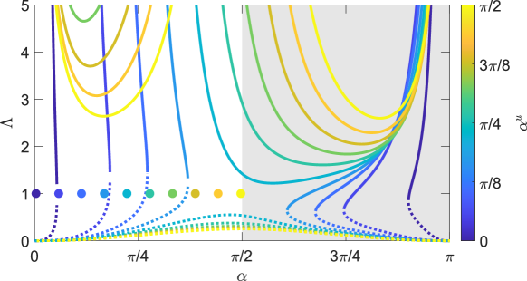
Figure 3: The branches of critical points on the $(\alpha,\Lambda)$ phase-plane, where the matrix of stiffness coefficients is singular: for each value of $\alpha^{u}$ (shown by the colourbar), we plot the real roots $\Lambda_{-}$ (solid curves) and $\Lambda_{+}$ (dotted curves), defined in Eq. (78), as $\alpha$ varies (here $\nu=1/3$). The point $(\alpha,\Lambda)=(\alpha^{u},1)$, corresponding to the undeformed configuration, is also plotted (circles). The unphysical region $\alpha\geq\pi/2$ is shaded.

More precisely, it may be shown that the discriminant attains its minimum value at $\alpha=\pi/2$, for any values of $\alpha^{u}$ and $\nu$. By considering the minimum value as a function of $\alpha^{u}$, we find that the discriminant is positive at $\alpha=\pi/2$ (and hence the roots are real across the entire interval $0<\alpha<\pi/2$) if and only if

$$\alpha^{u}>\arctan\left[\frac{2\nu^{1/2}}{(1+\nu)^{3/2}}\right].$$

In this regime, as $\alpha^{u}$ increases further for fixed $\nu$, the local minimum that can be observed in the $\Lambda_{-}$ branches (solid curves in Fig. 3) for $\alpha<\pi/2$ decreases significantly, eventually reaching values around $2.5$ when $\alpha^{u}\approx\pi/2$. In contrast, the $\Lambda_{+}$ branches (dotted curves) generally remain smaller than unity and decrease slightly as $\alpha^{u}$ increases. This behaviour as $\alpha^{u}$ varies has implications for the physical relevance of the critical points, as discussed later in §7.2.

4.4 Linearised equations: $\epsilon L\ll 1$

Up to this point, we have considered the case $\epsilon L=O(1)$, in which the changes to the helical parameters may be comparable to the undeformed values. This means that while the evolution equations are quasi-linear (i.e., linear in the first-order derivatives of $\alpha$ and $\Lambda$, or the second-order derivatives of $\mathcal{Z}$ and $\varPsi$), the coefficients are nonlinear functions of the solution variables, so that analytical progress is generally not possible. We therefore consider here the additional simplification of relatively short or stiff filaments, $L\ll\epsilon^{-1}$, for which the deformation is small and we can linearise the effective-column equations about the undeformed geometry.

Considering the formulation in terms of helix angle and contour wavelength, we write

$$\alpha(\mathcal{S},T)=\alpha^{u}+\Delta\alpha(\mathcal{S},T),\quad\Lambda(\mathcal{S},T)=1+\Delta\Lambda(\mathcal{S},T),$$

where $\Delta\alpha,\ \Delta\Lambda=O(\epsilon L)\ll 1$. Neglecting terms of $O(\epsilon L)^{2}$, Eqs. (67)–(68) and boundary conditions (70) simplify to

$$C_{1}^{u}\frac{\partial\Delta\alpha}{\partial\mathcal{S}}+C_{2}^{u}\frac{\partial\Delta\Lambda}{\partial\mathcal{S}}+\overline{\mathbf{e}_{z}\cdot\mathbf{F}_{e}^{(0)}}+\sin\alpha^{u}\int_{0}^{\mathcal{S}}\frac{\partial^{2}\Delta\alpha}{\partial T^{2}}\Bigg{\lvert}_{\mathcal{S}=\xi}\mathrm{d}\xi=0,$$ (79)

$$C_{3}^{u}\frac{\partial\Delta\alpha}{\partial\mathcal{S}}+C_{4}^{u}\frac{\partial\Delta\Lambda}{\partial\mathcal{S}}+\delta\overline{\mathbf{e}_{z}\cdot\mathbf{M}_{e}^{(0)}}+\frac{\sin\alpha^{u}}{2\pi}\overline{\mathbf{e}_{\theta}\cdot\mathbf{F}_{e}^{(0)}}+\frac{h\sin^{2}\alpha^{u}}{2\pi}\int_{0}^{\mathcal{S}}\frac{\partial^{2}\Delta\Lambda}{\partial T^{2}}\Bigg{\lvert}_{\mathcal{S}=\xi}\mathrm{d}\xi=0,$$ (80)

$$\Delta\alpha(\epsilon L,T)=\Delta\Lambda(\epsilon L,T)=0,$$ (81)

where the linearised stiffness coefficients are

$$C_{1}^{u}=-\frac{4\pi^{2}\csc\alpha^{u}\left(1+\nu\cos^{2}\alpha^{u}\right)}{1+\nu},\quad C_{2}^{u}=\frac{4\pi^{2}\nu\cos\alpha^{u}}{1+\nu},\quad C_{3}^{u}=\frac{2\pi h\nu\cos\alpha^{u}\sin\alpha^{u}}{1+\nu},\quad C_{4}^{u}=-\frac{2\pi h\left(1+\nu\sin^{2}\alpha^{u}\right)}{1+\nu}.$$ (82)

Alternatively, Eqs. (79)–(80) can be derived directly from Eqs. (62)–(63) by substituting expressions for the linearised resultant force, $F_{Z}$, and moment, $M_{Z}$; using Eq. (66), the linearised resultants are given by

$$F_{Z}\sim\frac{4\pi^{2}\left[\nu\Delta\Lambda\cos\alpha^{u}-\Delta\alpha\csc\alpha^{u}\left(1+\nu\cos^{2}\alpha^{u}\right)\right]}{1+\nu},\quad M_{Z}\sim\frac{2\pi h\left[\nu\Delta\alpha\cos\alpha^{u}\sin\alpha^{u}-\Delta\Lambda\left(1+\nu\sin^{2}\alpha^{u}\right)\right]}{1+\nu}.$$ (83)

We note that the Jacobian determinant of the linearised system, $J^{u}$, is

$$J^{u}=C_{1}^{u}C_{4}^{u}-C_{2}^{u}C_{3}^{u}=\frac{8\pi^{3}h\csc\alpha^{u}}{1+\nu}\neq 0.$$ (84)

The (steady) linearised system therefore does not exhibit singular behaviour, as is also evidenced by the fact that, for each $\alpha^{u}$, the undeformed point $(\alpha^{u},1)$ lies away from the branches of critical points in Fig. 3.

When the inertia terms are negligible, we can solve the system (79)–(80) uniquely for $\partial\Delta\alpha/\partial\mathcal{S}$ and $\partial\Delta\Lambda/\partial\mathcal{S}$, and formally integrate with the boundary conditions (81). After substituting the expressions for the coefficients $C_{i}^{u}$, we obtain

$$\Delta\alpha =-\int_{\mathcal{S}}^{\epsilon L}\left[\frac{\sin\alpha^{u}\left(1+\nu\sin^{2}\alpha^{u}\right)}{4\pi^{2}}\overline{\mathbf{e}_{z}\cdot\mathbf{F}_{e}^{(0)}}\Big{\lvert}_{\mathcal{S}=\xi}+\frac{h\nu\cos\alpha^{u}\sin\alpha^{u}}{2\pi}\left(\delta\overline{\mathbf{e}_{z}\cdot\mathbf{M}_{e}^{(0)}}+\frac{\sin\alpha^{u}}{2\pi}\overline{\mathbf{e}_{\theta}\cdot\mathbf{F}_{e}^{(0)}}\right)\Bigg{\lvert}_{\mathcal{S}=\xi}\right]\mathrm{d}\xi,$$

$$\Delta\Lambda =-\int_{\mathcal{S}}^{\epsilon L}\left[\frac{\nu\cos\alpha^{u}\sin^{2}\alpha^{u}}{4\pi^{2}}\overline{\mathbf{e}_{z}\cdot\mathbf{F}_{e}^{(0)}}\Big{\lvert}_{\mathcal{S}=\xi}+\frac{h\left(1+\nu\cos^{2}\alpha^{u}\right)}{2\pi}\left(\delta\overline{\mathbf{e}_{z}\cdot\mathbf{M}_{e}^{(0)}}+\frac{\sin\alpha^{u}}{2\pi}\overline{\mathbf{e}_{\theta}\cdot\mathbf{F}_{e}^{(0)}}\right)\Bigg{\lvert}_{\mathcal{S}=\xi}\right]\mathrm{d}\xi.$$ (85)

Using Eq. (34), the corresponding (linearised) wavelength-averaged longitudinal coordinate and winding angle are

$$\mathcal{Z} =\mathcal{S}\cos\alpha^{u}+\int_{0}^{\mathcal{S}}\int_{\eta}^{\epsilon L}\left[\frac{\sin^{2}\alpha^{u}\left(1+\nu\sin^{2}\alpha^{u}\right)}{4\pi^{2}}\overline{\mathbf{e}_{z}\cdot\mathbf{F}_{e}^{(0)}}\Big{\lvert}_{\mathcal{S}=\xi}+\frac{h\nu\cos\alpha^{u}\sin^{2}\alpha^{u}}{2\pi}\left(\delta\overline{\mathbf{e}_{z}\cdot\mathbf{M}_{e}^{(0)}}+\frac{\sin\alpha^{u}}{2\pi}\overline{\mathbf{e}_{\theta}\cdot\mathbf{F}_{e}^{(0)}}\right)\Bigg{\lvert}_{\mathcal{S}=\xi}\right]\mathrm{d}\xi\mathrm{d}\eta,$$

$$\varPsi =2\pi h\mathcal{S}+\int_{0}^{\mathcal{S}}\int_{\eta}^{\epsilon L}\left[\frac{h\nu\cos\alpha^{u}\sin^{2}\alpha^{u}}{2\pi}\overline{\mathbf{e}_{z}\cdot\mathbf{F}_{e}^{(0)}}\Big{\lvert}_{\mathcal{S}=\xi}+\left(1+\nu\cos^{2}\alpha^{u}\right)\left(\delta\overline{\mathbf{e}_{z}\cdot\mathbf{M}_{e}^{(0)}}+\frac{\sin\alpha^{u}}{2\pi}\overline{\mathbf{e}_{\theta}\cdot\mathbf{F}_{e}^{(0)}}\right)\Bigg{\lvert}_{\mathcal{S}=\xi}\right]\mathrm{d}\xi\mathrm{d}\eta.$$ (86)

4.5 Comparison with past work

We show in this section that the linearised effective-column equations, when written in terms of the wavelength-averaged longitudinal and rotational displacements, recover the equations previously proposed for helical coil springs (Phillips and Costello, 1972; Jiang et al., 1989, 1991). We write

$$\mathcal{Z}(\mathcal{S},T)=\mathcal{S}\cos\alpha^{u}+\Delta\mathcal{Z}(\mathcal{S},T),\quad\varPsi(\mathcal{S},T)=2\pi h\mathcal{S}+\Delta\varPsi(\mathcal{S},T),$$

where $\Delta\mathcal{Z},\ \Delta\varPsi=O(\epsilon L)\ll 1$. The effective-column equations (72)–(73) and boundary conditions (75)–(76) then become, neglecting terms of $O(\epsilon L)^{2}$,

$$K_{1}^{u}\frac{\partial^{2}\Delta\mathcal{Z}}{\partial\mathcal{S}^{2}}+K_{2}^{u}\frac{\partial^{2}\Delta\varPsi}{\partial\mathcal{S}^{2}}+\overline{\mathbf{e}_{z}\cdot\mathbf{F}_{e}^{(0)}}-\frac{\partial^{2}\Delta\mathcal{Z}}{\partial T^{2}}=0,$$ (87)

$$K_{3}^{u}\frac{\partial^{2}\Delta\mathcal{Z}}{\partial\mathcal{S}^{2}}+K_{4}^{u}\frac{\partial^{2}\Delta\varPsi}{\partial\mathcal{S}^{2}}+\delta\overline{\mathbf{e}_{z}\cdot\mathbf{M}_{e}^{(0)}}+\frac{\sin\alpha^{u}}{2\pi}\overline{\mathbf{e}_{\theta}\cdot\mathbf{F}_{e}^{(0)}}-\frac{\sin^{2}\alpha^{u}}{4\pi^{2}}\frac{\partial^{2}\Delta\varPsi}{\partial T^{2}}=0,$$ (88)

$$\Delta\mathcal{Z}(0,T)=\Delta\varPsi(0,T)=0,\quad\frac{\partial\Delta\mathcal{Z}}{\partial\mathcal{S}}(\epsilon L,T)=\frac{\partial\Delta\varPsi}{\partial\mathcal{S}}(\epsilon L,T)=0,$$ (89)

where

$$K_{1}^{u}=\frac{4\pi^{2}\csc^{2}\alpha^{u}\left(1+\nu\cos^{2}\alpha^{u}\right)}{1+\nu},\quad K_{2}^{u}=K_{3}^{u}=-\frac{2\pi h\nu\cos\alpha^{u}}{1+\nu},\quad K_{4}^{u}=\frac{1+\nu\sin^{2}\alpha^{u}}{1+\nu}.$$ (90)

Equations (87)–(88) can also be derived directly from Eqs. (62)–(63) by substituting expressions for the linearised resultant force, $F_{Z}$, and moment, $M_{Z}$, in terms of $\Delta\mathcal{Z}$ and $\Delta\varPsi$; these expressions can be obtained from Eq. (83) and noting from Eq. (71) that the perturbations $(\Delta\alpha,\Delta\Lambda)$ are related to $(\Delta\mathcal{Z},\Delta\varPsi)$ by

$$\Delta\alpha=-\csc\alpha^{u}\frac{\partial\Delta\mathcal{Z}}{\partial\mathcal{S}},\quad\Delta\Lambda=-\frac{1}{2\pi h}\frac{\partial\Delta\varPsi}{\partial\mathcal{S}}.$$ (91)

Recall from Eqs. (32)–(33) that $\mathcal{Z}$ and $\varPsi$ represent the $O(\epsilon^{-1})$ contribution to the dimensionless longitudinal coordinate and winding angle, respectively. Hence, in unscaled variables, the wavelength-averaged extensional and rotational displacements are

$$\Delta z=\frac{\lambda^{u}}{\epsilon}\Delta\mathcal{Z},\quad\Delta\Psi=\frac{1}{\epsilon}\Delta\varPsi.$$

From the re-scalings introduced in Eq. (13) and Eqs. (25)–(26), we have $s=\lambda^{u}S=\epsilon^{-1}\lambda^{u}\mathcal{S}$ and $t=[t]T=\epsilon^{-1}t^{*}T$. Setting $\mathbf{f}_{e}^{(0)}=[f]\mathbf{F}_{e}^{(0)}$ and $\mathbf{m}_{e}^{(0)}=[m]\mathbf{M}_{e}^{(0)}$, and making use of the expressions (20) for $\epsilon$, $\delta$ and $t^{*}$, Eqs. (87)–(89) in terms of dimensional variables are

$$k_{1}^{u}\frac{\partial^{2}\Delta z}{\partial s^{2}}+k_{2}^{u}\frac{\partial^{2}\Delta\Psi}{\partial s^{2}}+\overline{\mathbf{e}_{z}\cdot\mathbf{f}_{e}^{(0)}}-\rho_{s}A\frac{\partial^{2}\Delta z}{\partial t^{2}}=0,$$ (92)

$$k_{3}^{u}\frac{\partial^{2}\Delta z}{\partial s^{2}}+k_{4}^{u}\frac{\partial^{2}\Delta\Psi}{\partial s^{2}}+\overline{\mathbf{e}_{z}\cdot\mathbf{m}_{e}^{(0)}}+r^{u}\overline{\mathbf{e}_{\theta}\cdot\mathbf{f}_{e}^{(0)}}-\rho_{s}A\left(r^{u}\right)^{2}\frac{\partial^{2}\Delta\Psi}{\partial t^{2}}=0,$$ (93)

$$\Delta z(0,t)=\Delta\Psi(0,t)=0,\quad\frac{\partial\Delta z}{\partial s}(l,t)=\frac{\partial\Delta\Psi}{\partial s}(l,t)=0,$$ (94)

where, using $r^{u}=\lambda^{u}\sin\alpha^{u}/(2\pi)$,

$$k_{1}^{u}=\frac{BK_{1}^{u}}{\left(\lambda^{u}\right)^{2}}=\frac{B\left(1+\nu\cos^{2}\alpha^{u}\right)}{(1+\nu)\left(r^{u}\right)^{2}},\quad k_{2}^{u}=k_{3}^{u}=\frac{BK_{2}^{u}}{\lambda^{u}}=-\frac{h\nu B\cos\alpha^{u}\sin\alpha^{u}}{(1+\nu)r^{u}},\quad k_{4}^{u}=BK_{4}^{u}=\frac{B\left(1+\nu\sin^{2}\alpha^{u}\right)}{1+\nu}.$$ (95)

In the absence of external loads, Eqs. (92)–(93) are equivalent to the linearised equations proposed by Phillips and Costello (1972) to model the free vibrations of helical coil springs; we also recover the linearised equations later reported by Jiang et al. (1989, 1991), once their stiffness coefficients are expanded in the inextensible limit $a\ll r^{u}$ considered here. In these studies, the dynamic equations were obtained by considering the equilibrium solution of a helical filament under a constant wrench aligned with the helix axis, determining effective stiffness coefficients from this solution, then making the ad hoc assumption that the stiffness coefficients can be applied locally when balancing linear and angular momentum for each infinitesimal spring element. Our multiple-scales analysis therefore rigorously justifies this assumption for problems involving unsteady deformations and distributed loads.

4.6 Effective-column equations in the straight-rod limit, $\alpha^{u}\to 0$

In this final subsection, we briefly discuss the limit of vanishing pitch angle. For simplicity, we focus on the linearised effective-column equations in terms of the (dimensional) wavelength-averaged displacements, i.e., Eqs. (92)–(93). As $\alpha^{u}\to 0$ for fixed $\lambda^{u}$, the coefficients $k_{i}^{u}$ in Eq. (95) take the limiting form

$$k_{1}^{u}\sim\frac{4\pi^{2}B}{\left(\lambda^{u}\alpha^{u}\right)^{2}},\quad k_{2}^{u}=k_{3}^{u}\sim-\frac{2\pi h\nu B}{(1+\nu)\lambda^{u}},\quad k_{4}^{u}\sim\frac{B}{1+\nu}.$$

Because $k_{1}^{u}\to\infty$, if we assume that the external force $\mathbf{f}_{e}^{(0)}$ and accelerations $\partial^{2}\Delta z/\partial t^{2}$ remain bounded as $\alpha^{u}\to 0$, Eq. (92) requires that $\partial^{2}\Delta z/\partial s^{2}\approx 0$ and hence, from the boundary conditions (94), $\Delta z\approx 0$ throughout the filament. Equation (93) then reduces to

$$C\frac{\partial^{2}\Delta\Psi}{\partial s^{2}}+\overline{\mathbf{e}_{z}\cdot\mathbf{m}_{e}^{(0)}}=0,$$

recalling from Eq. (10) that $C=B/(1+\nu)$ is the twist modulus. We see that the effective moment resultant (about the helix axis) is $m_{z}=C\left(\partial\Delta\Psi/\partial s\right)$; hence, it is precisely the gradient of the winding angle, $\partial\Delta\Psi/\partial s$, which maps onto axial (excess) twist of the limiting straight rod. This is a consequence of the fact that the straight-rod limit $\alpha^{u}\to 0$ here is taken with $\lambda^{u}$ and $a$ fixed, i.e., the helix radius $r^{u}=\lambda^{u}\sin\alpha^{u}/(2\pi)\to 0$ while the cross-section radius is constant, so that rotation of the centreline about the helix axis becomes equivalent to axial twist. We note that a term $\partial^{2}\Delta\Psi/\partial t^{2}$, which is present when modelling torsional vibrations in a straight rod, does not appear here because we neglected rotary inertia in the moment balance (21).

We also deduce that, under the assumption that the filament tip is free of forces and moments, non-trivial equilibrium solutions are only possible as $\alpha^{u}\to 0$ (with $\lambda^{u}$ and $a$ fixed) if the external moment $\mathbf{m}_{e}^{(0)}$ is non-zero. This can be traced back to the inextensibility assumption: there cannot be any longitudinal displacement of the straight rod and hence the force balance is not relevant in the straight-rod limit.

5 Physical scenario I: The heavy helical column

The first specific physical scenario we analyse is a helical filament deforming under its own weight. As in previous sections, the filament is supported at its base such that the helix axis is directed along $\mathbf{e}_{z}$, with the other end free. To be consistent with our assumption that the helix axis remains straight, we assume that the gravitational field is parallel to $\mathbf{e}_{z}$ and we focus on equilibrium solutions; the solvability conditions in Eq. (64) are then satisfied. This scenario is analogous to the classic problem studied by Greenhill (1881) for a straight column, though we do not address the stability of solutions or bending of the helix axis here.

5.1 Governing equations

The external force and moment (per unit arclength) are $\mathbf{f}_{e}=\rho_{s}Ag\,\mathbf{e}_{z}$ and $\mathbf{m}_{e}=\mathbf{0}$, respectively, where $g$ is the gravitational acceleration in the direction of increasing $z$: if $g>0$ the filament is under tension, and if $g<0$ the filament is under compression. To non-dimensionalise, we use the force scale $[f]=\rho_{s}A|g|$ in the re-scalings introduced in Eq. (13), which gives

$$\epsilon=\frac{\rho_{s}A|g|\left(\lambda^{u}\right)^{3}}{B},\quad\delta=0,\quad\mathbf{F}_{e}=\mathbf{F}_{e}^{(0)}=\operatorname{sgn}g\,\mathbf{e}_{z}.$$ (96)

We note that the highly-coiled assumption ($\epsilon\ll 1$) in this context reads $\lambda^{u}\ll[s]=\left[B/\left(\rho_{s}A|g|\right)\right]^{1/3}$, where $[s]$ is the elasto-gravity length that frequently arises in problems involving rods bending under self-weight (Wang, 1986).

We use the dimensionless formulation of the effective-column equations in terms of the slowly-varying pitch angle, $\alpha$, and wavelength, $\Lambda$, i.e., Eqs. (67)–(68). Neglecting time derivatives, these equations become

$$C_{1}\frac{\partial\alpha}{\partial\mathcal{S}}+C_{2}\frac{\partial\Lambda}{\partial\mathcal{S}}+\operatorname{sgn}g=0,$$ (97)

$$C_{3}\frac{\partial\alpha}{\partial\mathcal{S}}+C_{4}\frac{\partial\Lambda}{\partial\mathcal{S}}=0,$$ (98)

to be solved with the boundary conditions (70).

5.2 Linearised solution: $\epsilon L\ll 1$

While the deformation remains small, the general solution of the linearised equations, Eq. (85) (determined earlier in §4.4), becomes

$$\Delta\alpha=-\frac{\sin\alpha^{u}\left(1+\nu\sin^{2}\alpha^{u}\right)\operatorname{sgn}g}{4\pi^{2}}\left(\epsilon L-\mathcal{S}\right),\quad\Delta\Lambda=-\frac{\nu\cos\alpha^{u}\sin^{2}\alpha^{u}\operatorname{sgn}g}{4\pi^{2}}\left(\epsilon L-\mathcal{S}\right).$$ (99)

A few features of this solution are noteworthy. Firstly, due to linearisation and the fact that the external force is independent of the solution, the perturbations have the symmetry $(\Delta\alpha,\Delta\Lambda)\to-(\Delta\alpha,\Delta\Lambda)$ as $g\to-g$. Because the filament tip at $\mathcal{S}=\epsilon L$ is free and there are no other boundary conditions for $\alpha$ and $\Lambda$ (in particular, there are no unknown parameters that depend on the value of the solution away from the tip), the linearised solution is always valid near the tip, even if $\epsilon L=O(1)$. In particular, $\Delta\alpha$ and $\Delta\Lambda$ remain much smaller than unity provided

$$\left(\epsilon L-\mathcal{S}\right)\ll 1.$$

If $\epsilon L\ll 1$, the linearised solution is then valid throughout the entire length of the filament. Furthermore, we note that, in the straight-rod limit $\alpha^{u}\to 0$ (with $\lambda^{u}$ fixed), the perturbation $\Delta\alpha\to 0$ because of rod inextensibility and $\Delta\Lambda\to 0$ because no external moment is applied (recall the discussion in §4.6).

From Eq. (86), the corresponding wavelength-averaged longitudinal coordinate and winding angle are given by

$$\mathcal{Z}=\mathcal{S}\cos\alpha^{u}+\frac{\sin^{2}\alpha^{u}\left(1+\nu\sin^{2}\alpha^{u}\right)\operatorname{sgn}g}{8\pi^{2}}\>\mathcal{S}\left(2\epsilon L-\mathcal{S}\right),\quad\varPsi=2\pi h\mathcal{S}+\frac{h\nu\cos\alpha^{u}\sin^{2}\alpha^{u}\operatorname{sgn}g}{4\pi}\>\mathcal{S}\left(2\epsilon L-\mathcal{S}\right).$$

We see that the perturbations $\Delta\mathcal{Z}\equiv\mathcal{Z}-\mathcal{S}\cos\alpha^{u}$ and $\Delta\varPsi\equiv\varPsi-2\pi h\mathcal{S}$ vary quadratically with the slow variable, $\mathcal{S}$, and, as expected, their magnitude is largest at the filament tip, $\mathcal{S}=\epsilon L$.

5.3 General solution: $\epsilon L=O(1)$

When the deformation is no longer small, it is not possible to solve Eqs. (97)–(98) analytically so we appeal to numerical integration. We recast the equations as an initial-value problem by introducing

$$\Xi=\epsilon L-\mathcal{S},\qquad\Xi\in[0,\epsilon L],$$

so that the boundary conditions (70) at the filament tip become initial conditions at $\Xi=0$. For specified values of the dimensionless parameters (namely $\operatorname{sgn}g$, $\alpha^{u}$, $\nu$ and $h$), we numerically integrate Eqs. (97)–(98) up to some maximum value $\Xi=\Xi_{\mathrm{max}}$; the solution for any $\epsilon L\leq\Xi_{\mathrm{max}}$ can then be found by truncating the trajectories at $\Xi=\epsilon L$.

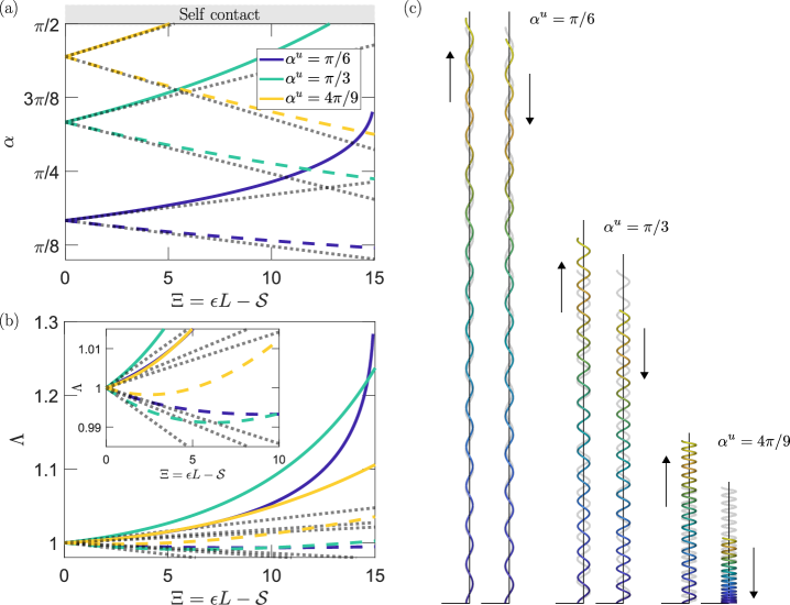
Figure 4: The heavy helical column: the deformation of a highly-coiled helical rod due to a gravitational field parallel to the helix axis (here $\nu=1/3$ and $h=-1$). We plot trajectories of (a) the slowly-varying pitch angle, $\alpha$; and (b) the dimensionless helical wavelength, $\Lambda=\lambda/\lambda^{u}$, obtained by numerically integrating Eqs. (97)–(98) with boundary conditions (70). In panels (a)–(b), the solutions are plotted as a function of dimensionless arclength from the filament tip, $\Xi=\epsilon L-\mathcal{S}$, for three different values of the undeformed pitch angle $\alpha^{u}$ (see legend) and either $g>0$ (dashed curves) or $g<0$ (solid curves). Also shown are the corresponding linearised solutions (99) (grey dotted lines), formally valid for $\Xi\ll 1$. (c) Numerical shapes (side view), corresponding to the solutions in (a)–(b) at $\epsilon L=4.5$ (taking $L=15$, $\epsilon=0.3$). Arrows indicate the direction of gravity.

In Figs. 4a–b, we plot typical trajectories of $\alpha$ and $\Lambda$ as a function of $\Xi$, both for $g>0$ (filament under tension; dashed curves) and $g<0$ (filament under compression; solid curves). Even though the linearised solution in Eq. (99) (grey dotted lines in Figs. 4a–b) is formally valid only for $\Xi\ll 1$, we see that it performs excellently up to $\Xi\approx 1$. In the regime $\Xi\lesssim 1$, the symmetry in the perturbations $\Delta\alpha=\alpha-\alpha^{u}$ and $\Delta\Lambda=\Lambda-1$ as $g\to-g$ is also evident. However, at larger values of $\Xi$, the perturbations are no longer small and the numerical trajectories deviate significantly from the linearised solution. In particular, because the coefficients $C_{i}$ in Eqs. (97)–(98) depend nonlinearly on the values of $\alpha$ and $\Lambda$, the symmetry in the solutions as $g\to-g$ is no longer present. The nonlinear dependence of the coefficients $C_{i}$ is also responsible for the non-monotonic variation of the wavelength $\Lambda$ observed when $g>0$ (Fig. 4b inset): $\Lambda$ decreases slightly before increasing again, corresponding to winding then unwinding, which is a generic phenomenon for helical filaments under longitudinal forces (Goriely, 2017). The corresponding shapes of the filament at $\epsilon L=4.5$ are shown in Fig. 4c, determined by integrating the tangent vector $\mathbf{d}_{3}^{(0)}=\mathbf{t}$ evaluated using Eq. (28).

Another key feature observed in Figs. 4a–b is that the solution becomes singular if $g<0$ and $\alpha^{u}$ is sufficiently small: the numerical trajectory for $\alpha^{u}=\pi/6$ reaches a point of vertical tangency at $\Xi\approx 15$ and it is not possible to integrate further. (For larger values of $\alpha^{u}$, self-contact occurs before any singularity.) To gain further understanding, Fig. 5 shows a density plot (‘heat map’) of the magnitude of the gradient vector associated with Eqs. (97)–(98), i.e., $\|(\partial\alpha/\partial\mathcal{S},\partial\Lambda/\partial\mathcal{S})\|$, which is plotted on the $(\alpha,\Lambda)$-plane together with phase trajectories (white arrows). When $g<0$, these arrows point in the direction of increasing $\Xi$, i.e., moving away from the filament tip; while when $g>0$, the arrows point in the direction of decreasing $\Xi$. Figure 5 confirms that the singularity observed in Figs. 4a–b corresponds to a critical point where the Jacobian determinant $\det J=C_{1}C_{4}-C_{2}C_{3}$ vanishes (black curves) and the magnitude of the gradient vector is infinite; we discussed the general existence of such critical points in §4.3. Also plotted on Fig. 5 is the trajectory emerging from $(\alpha,\Lambda)=(\alpha^{u},1)$ (red curves), corresponding to the solution satisfying the boundary conditions (70) at the filament tip, $\Xi=0$; this solution evidently only becomes singular in the physical region $\Xi>0$ when $g<0$, i.e., under compression. Nevertheless, we emphasise that near critical points, the solution varies rapidly with $\Xi$ and our multiple-scales analysis is not asymptotically valid (we discuss this point further in §7.2).

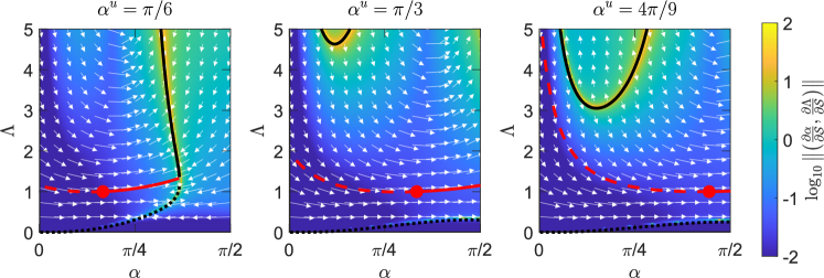
Figure 5: The heavy helical column: the phase plane of Eqs. (97)–(98) ($\nu=1/3$ and $h=-1$). In each panel, corresponding to a different undeformed pitch angle $\alpha^{u}$, phase trajectories (white arrows) are shown; arrows point in the direction of increasing (decreasing) arclength from the filament tip when $g<0$ ($g>0$), corresponding to the filament under compression (tension). The trajectory emerging from the undeformed point $(\alpha^{u},1)$ (red circle) is highlighted red. These trajectories are superimposed on a density plot of the local gradient vector $(\partial\alpha/\partial\mathcal{S},\partial\Lambda/\partial\mathcal{S})$, coloured according to the logarithm of its magnitude (see colourbar). Also shown are the branches of critical points $\Lambda_{-}$ (black solid curves) and $\Lambda_{+}$ (black dotted curves) from Eq. (78), at which the matrix of stiffness coefficients is singular and the magnitude of the local gradient vector is infinite.

While the singularity in the system only occurs under compression for large deformations $\epsilon L\gtrsim 15$, in practice the helix axis will buckle first, meaning our assumption of a straight axis is no longer valid. More precisely, in AppendixD we estimate the buckling threshold of a helical filament using an ad hoc effective-beam approximation, which indicates that buckling should occur well before $\epsilon L\approx 15$ for $\alpha^{u}\lesssim\pi/6$. However, it may be possible to reach values $\epsilon L\gtrsim 15$ with a straight helix axis if axial bending is prevented, for example by confining the filament radially. As discussed in §7.2, a radial contact force could be incorporated into our analysis without much difficulty.

6 Physical scenario II: Axial rotation (twirling) in viscous fluid

In the second physical scenario, we assume that the filament is immersed in viscous fluid and is rotated at its base about the helix axis at some prescribed angular frequency, $\omega_{0}$, while its other end is free; see Fig. 6. This may be considered as a simple model for a bacteria flagellar filament in which (i) the filament base is tethered in the laboratory frame, i.e., not freely swimming; (ii) we neglect the flexible ‘hook’ joint and tapered part connecting the rotary motor to the filament base (Higdon, 1979; Park et al., 2017), but incorporate their effect as transmitting a wrench to the filament needed to achieve the prescribed frequency, $\omega_{0}$; and (iii) polymorphic transformations away from the so-called ‘normal’ helical form do not occur (Hasegawa et al., 1998). Here we describe how the effective-column equations can be applied to this problem.

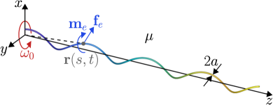
Figure 6: Schematic diagram of axial rotation (twirling) in viscous fluid: the helical filament is driven at its base at a prescribed angular frequency $\omega_{0}$ relative to fluid (viscosity $\mu$) in the laboratory frame. The hydrodynamic loading comprises a distributed force $\mathbf{f}_{e}$ and moment $\mathbf{m}_{e}$.

6.1 Governing equations

Since inertial forces are dominated by viscous forces at the small lengthscales characteristic of bacterial flagella (Powers, 2010), we neglect inertia of both the fluid and rod. We may then use resistive-force theory to compute the hydrodynamic forces and moments exerted on the filament (Lauga, 2020). While this theory neglects long-range hydrodynamic interactions arising from the curved geometry of the helix, it can be obtained as the asymptotic limit of slender-body theory when the cross-section radius $a$ is much smaller than the typical radius of curvature of the rod (Cox, 1970; Leal, 2007). For the helical filament considered here, this radius of curvature is of size $\lambda^{u}$ so the asymptotic limit is equivalent to $a\ll\lambda^{u}$, which is precisely the assumption we made in §2 to neglect axial extensibility.

Recall from §2.3 that the helix frame $Oxyz$ is defined such that the filament base (at $z=0$) is always located on the $x$-axis. The velocity of a point $\mathbf{r}$ on the filament centreline, relative to the fluid in the laboratory frame, is then

$$\mathbf{v}=\omega_{0}\mathbf{e}_{z}\times\mathbf{r}+\frac{\partial\mathbf{r}}{\partial t}.$$ (100)

The final term here, which accounts for motions relative to the helix frame, incorporates both spatial variation in the rotation rate and motions parallel to the helix axis. From resistive-force theory, the viscous drag force (per unit length) is given by (Lauga, 2020)

$$\mathbf{f}_{e}=-\zeta_{\parallel}\left(\mathbf{d}_{3}\cdot\mathbf{v}\right)\mathbf{d}_{3}-\zeta_{\perp}\left[\mathbf{v}-\left(\mathbf{d}_{3}\cdot\mathbf{v}\right)\mathbf{d}_{3}\right],$$ (101)

where, for a helical rod, the local drag coefficients for motion parallel and perpendicular to the rod centreline are given by Lighthill’s corrected coefficients (Lighthill, 1976):

$$\zeta_{\parallel}=\frac{2\pi\mu}{\log\left(0.18\lambda^{u}/a\right)},\quad\zeta_{\perp}=\frac{4\pi\mu}{\log\left(0.18\lambda^{u}/a\right)+1/2}.$$

Here $\mu$ is the dynamic viscosity of the fluid and we neglect small changes to the drag coefficients arising from variations in the contour wavelength. The fluid also exerts a moment (per unit length) opposing rotation of the filament cross-section:

$$\mathbf{m}_{e}=-4\pi\mu a^{2}\left(\mathbf{d}_{3}\cdot\left[\omega_{0}\mathbf{e}_{z}+\boldsymbol{\omega}\right]\right)\mathbf{d}_{3},$$ (102)

where $4\pi\mu a^{2}$ is the rotational drag coefficient (per unit length) of a rod with radius $a$ (Landau and Lifshitz, 1987), and $\boldsymbol{\omega}$ is the angular velocity vector (in the helix frame) introduced in Eq. (2).

To non-dimensionalise, we expect that the relevant velocity scale is the tangential velocity associated with the imposed rotation, i.e., $|\mathbf{v}|\sim\lambda^{u}|\omega_{0}|$. From Eqs. (101)–(102), it is then natural to choose the force and moment scales

$$[f]=\zeta_{\perp}\lambda^{u}|\omega_{0}|,\quad[m]=4\pi\mu a^{2}|\omega_{0}|.$$

The dimensionless parameters $\epsilon$ and $\delta$, defined in Eq. (20), are then given by

$$\epsilon=\frac{\zeta_{\perp}\left(\lambda^{u}\right)^{4}|\omega_{0}|}{B},\quad\delta=\frac{4\pi\mu a^{2}}{\zeta_{\perp}\left(\lambda^{u}\right)^{2}}.$$

With the above force scale $[f]$ and moment scale $[m]$, we introduce dimensionless variables as in §2 (Eq. (13)). Because we neglect rod inertia here, we do not rescale time by the timescale $[t]=\epsilon^{-1}t^{*}$, as was done in §3–4. Instead, we consider the timescale over which the filament deforms due to the hydrodynamic load: balancing the $\partial\mathbf{r}/\partial t$ term in the velocity (100) with $|\mathbf{v}|\sim\lambda^{u}|\omega_{0}|$ (noting that $|\mathbf{r}|=O(l)=O(\lambda^{u}L)=O(\epsilon^{-1}\lambda^{u})$ for $\epsilon L=O(1)$), this timescale is $t\sim\epsilon^{-1}|\omega_{0}|^{-1}$. Re-scaling also the angular velocity by $1/t\sim\epsilon|\omega_{0}|$ here, we therefore set

$$t=\epsilon^{-1}|\omega_{0}|^{-1}\hat{T},\quad\mathbf{v}=\lambda^{u}|\omega_{0}|\mathbf{V},\quad\boldsymbol{\omega}=\epsilon|\omega_{0}|\,\hat{\boldsymbol{\Omega}}.$$ (103)

Equations (100)–(102) then become

$$\mathbf{V}=\operatorname{sgn}\omega_{0}\mathbf{e}_{z}\times\mathbf{R}+\epsilon\frac{\partial\mathbf{R}}{\partial\hat{T}},\quad\mathbf{F}_{e}=-(1-\chi)\left(\mathbf{d}_{3}\cdot\mathbf{V}\right)\mathbf{d}_{3}-\left[\mathbf{V}-\left(\mathbf{d}_{3}\cdot\mathbf{V}\right)\mathbf{d}_{3}\right],\quad\mathbf{M}_{e}=-\left[\mathbf{d}_{3}\cdot\left(\operatorname{sgn}\omega_{0}\mathbf{e}_{z}+\epsilon\,\hat{\boldsymbol{\Omega}}\right)\right]\mathbf{d}_{3},$$ (104)

where the local drag anisotropy is characterised by the dimensionless parameter

$$\chi=\frac{\zeta_{\perp}-\zeta_{\parallel}}{\zeta_{\perp}}\approx\frac{1}{2}.$$

We use the expressions in Eqs. (35) and (41) for the leading-order centreline velocity, $\partial\mathbf{R}^{(0)}/\partial T$, and angular velocity vector, $\boldsymbol{\Omega}^{(0)}$, in terms of variables characterising the locally-helical shape: the slowly-varying helical radius, $\mathcal{R}$, wavelength-averaged longitudinal coordinate, $\mathcal{Z}$, and wavelength-averaged winding angle, $\varPsi$. Noting that $\partial/\partial T=(|\omega_{0}|t^{*})\partial/\partial\hat{T}$ and $\boldsymbol{\Omega}=\epsilon^{-1}t^{*}\boldsymbol{\omega}=|\omega_{0}|t^{*}\hat{\boldsymbol{\Omega}}$, we obtain

$$\frac{\partial\mathbf{R}}{\partial\hat{T}}\sim\frac{\partial\mathbf{R}^{(0)}}{\partial\hat{T}}=\epsilon^{-1}\left(\mathcal{R}\frac{\partial\varPsi}{\partial\hat{T}}\mathbf{e}_{\theta}+\frac{\partial\mathcal{Z}}{\partial\hat{T}}\mathbf{e}_{z}\right)+O(1),\quad\hat{\boldsymbol{\Omega}}\sim\hat{\boldsymbol{\Omega}}^{(0)}=\epsilon^{-1}\frac{\partial\varPsi}{\partial\hat{T}}\mathbf{e}_{z}+O(1).$$ (105)

Using $\mathbf{d}_{3}\sim\mathbf{d}_{3}^{(0)}=\mathbf{t}=h\sin\alpha\,\mathbf{e}_{\theta}+\cos\alpha\,\mathbf{e}_{z}$ (recall Eqs. (28) and (31)), the external loads (104) to leading order (i.e., neglecting terms of $O(\epsilon)$) can be written in cylindrical polar coordinates as

$$\mathbf{F}_{e}^{(0)}= -\left[\mathcal{R}\left(1-\chi\sin^{2}\alpha\right)\left(\operatorname{sgn}\omega_{0}+\frac{\partial\varPsi}{\partial\hat{T}}\right)-h\chi\cos\alpha\sin\alpha\frac{\partial\mathcal{Z}}{\partial\hat{T}}\right]\mathbf{e}_{\theta}$$

$$\>-\left[\left(1-\chi\cos^{2}\alpha\right)\frac{\partial\mathcal{Z}}{\partial\hat{T}}-h\chi\mathcal{R}\cos\alpha\sin\alpha\left(\operatorname{sgn}\omega_{0}+\frac{\partial\varPsi}{\partial\hat{T}}\right)\right]\mathbf{e}_{z},\qquad$$

$$\mathbf{M}_{e}^{(0)}= -\cos\alpha\left(\operatorname{sgn}\omega_{0}+\frac{\partial\varPsi}{\partial\hat{T}}\right)\left(h\sin\alpha\,\mathbf{e}_{\theta}+\cos\alpha\,\mathbf{e}_{z}\right).$$

We note that the coefficients of $\mathbf{e}_{\theta}$ and $\mathbf{e}_{z}$ in the above expressions for $\mathbf{F}_{e}^{(0)}$ and $\mathbf{M}_{e}^{(0)}$ are independent of the fast variable, $S$. In particular, this means that the off-axis components of $\mathbf{F}_{e}^{(0)}$ average to zero over each wavelength, i.e., $\overline{\mathbf{e}_{x}\cdot\mathbf{F}_{e}^{(0)}}=0$ and $\overline{\mathbf{e}_{y}\cdot\mathbf{F}_{e}^{(0)}}=0$; because we also neglect inertial terms, the off-axis solvability conditions in Eq. (64) are then satisfied. We also calculate the component of the wavelength-averaged external force and moment along $\mathbf{e}_{z}$:

$$\overline{\mathbf{e}_{z}\cdot\mathbf{F}_{e}^{(0)}}=-A_{\parallel}\frac{\partial\mathcal{Z}}{\partial\hat{T}}-B_{\parallel}\left(\operatorname{sgn}\omega_{0}+\frac{\partial\varPsi}{\partial\hat{T}}\right),\quad\delta\overline{\mathbf{e}_{z}\cdot\mathbf{M}_{e}^{(0)}}+\mathcal{R}\overline{\mathbf{e}_{\theta}\cdot\mathbf{F}_{e}^{(0)}}=-B_{\parallel}\frac{\partial\mathcal{Z}}{\partial\hat{T}}-C_{\parallel}\left(\operatorname{sgn}\omega_{0}+\frac{\partial\varPsi}{\partial\hat{T}}\right),$$

where we define the drag coefficients

$$A_{\parallel}=1-\chi\cos^{2}\alpha,\quad B_{\parallel}=-h\chi\mathcal{R}\cos\alpha\sin\alpha,\quad C_{\parallel}=\delta\cos^{2}\alpha+\mathcal{R}^{2}\left(1-\chi\sin^{2}\alpha\right).$$

Substituting the above expressions into the effective-column equations (72)–(73) then yields a closed system of PDEs for $\mathcal{Z}(\mathcal{S},T)$ and $\varPsi(\mathcal{S},T)$, which, in the absence of the inertia terms, take the form of coupled diffusion equations. Because the drag coefficients generally depend on the (unknown) helical geometry, these equations are nonlinear; the drag coefficients and helical radius $\mathcal{R}$ can be written in terms of $\mathcal{Z}$ and $\varPsi$ using Eq. (71).

6.2 Linearised solution: $\epsilon L\ll 1$

In what follows, we restrict to small deformations, $\epsilon L\ll 1$, for which an analytical solution is possible. Neglecting inertia terms, the linearised effective-column equations (87)–(88) and boundary conditions (89) in terms of $\Delta\mathcal{Z}\equiv\mathcal{Z}-\mathcal{S}\cos\alpha^{u}$ and $\Delta\varPsi\equiv\varPsi-2\pi h\mathcal{S}$ become

$$K_{1}^{u}\frac{\partial^{2}\Delta\mathcal{Z}}{\partial\mathcal{S}^{2}}+K_{2}^{u}\frac{\partial^{2}\Delta\varPsi}{\partial\mathcal{S}^{2}}=A_{\parallel}^{u}\frac{\partial\Delta\mathcal{Z}}{\partial\hat{T}}+B_{\parallel}^{u}\left(\operatorname{sgn}\omega_{0}+\frac{\partial\Delta\varPsi}{\partial\hat{T}}\right),$$ (106)

$$K_{2}^{u}\frac{\partial^{2}\Delta\mathcal{Z}}{\partial\mathcal{S}^{2}}+K_{4}^{u}\frac{\partial^{2}\Delta\varPsi}{\partial\mathcal{S}^{2}}=B_{\parallel}^{u}\frac{\partial\Delta\mathcal{Z}}{\partial\hat{T}}+C_{\parallel}^{u}\left(\operatorname{sgn}\omega_{0}+\frac{\partial\Delta\varPsi}{\partial\hat{T}}\right),$$ (107)

$$\Delta\mathcal{Z}(0,\hat{T})=\Delta\varPsi(0,\hat{T})=0,\quad\frac{\partial\Delta\mathcal{Z}}{\partial\mathcal{S}}(\epsilon L,\hat{T})=\frac{\partial\Delta\varPsi}{\partial\mathcal{S}}(\epsilon L,\hat{T})=0,$$ (108)

where the drag coefficients are approximated by their undeformed values:

$$A_{\parallel}^{u}=1-\chi\cos^{2}\alpha^{u},\quad B_{\parallel}^{u}=-\frac{h\chi\cos\alpha^{u}\sin^{2}\alpha^{u}}{2\pi},\quad C_{\parallel}^{u}=\delta\cos^{2}\alpha^{u}+\frac{\sin^{2}\alpha^{u}}{4\pi^{2}}\left(1-\chi\sin^{2}\alpha^{u}\right).$$ (109)

For initial conditions, we suppose that the filament is undeformed at $\hat{T}=0$ before the rotation is instantaneously applied for $\hat{T}>0$:

$$\Delta\mathcal{Z}(\mathcal{S},0)=\Delta\varPsi(\mathcal{S},0)=0.$$ (110)

We note that, in the straight-rod limit $\alpha^{u}\to 0$ with $\lambda^{u}$ fixed, Eqs. (106)–(107) reduce to the classical equation governing twist diffusion in a straight rod (Wolgemuth et al., 2000) when we identify $\partial\Delta\varPsi/\partial\mathcal{S}$ with the axial twist (recall the discussion in §4.6).

We choose to write the system of equations in matrix-vector form by introducing the column vector $\mathcal{Y}\left(\mathcal{S},\hat{T}\right)=\left(\Delta\mathcal{Z},\Delta\varPsi\right)^{\mathrm{T}}$. Equations (106)–(108) and (110) can be written as

$$J^{u}\frac{\partial^{2}\mathcal{Y}}{\partial\mathcal{S}^{2}}=\Upsilon^{u}\left[\frac{\partial\mathcal{Y}}{\partial\hat{T}}+\begin{pmatrix}0\\ \operatorname{sgn}\omega_{0}\end{pmatrix}\right]\qquad\mathrm{where}\qquad J^{u}=\begin{pmatrix}K_{1}^{u}&K_{2}^{u}\\ K_{2}^{u}&K_{4}^{u}\end{pmatrix},\quad\Upsilon^{u}=\begin{pmatrix}A_{\parallel}^{u}&B_{\parallel}^{u}\\ B_{\parallel}^{u}&C_{\parallel}^{u}\end{pmatrix},$$ (111)

$$\mathcal{Y}\left(0,\hat{T}\right)=\mathsf{0}_{2\times 1},\quad\frac{\partial\mathcal{Y}}{\partial\mathcal{S}}\left(\epsilon L,\hat{T}\right)=\mathsf{0}_{2\times 1},\quad\mathcal{Y}\left(\mathcal{S},0\right)=\mathsf{0}_{2\times 1}.$$ (112)

Note that the matrices of undeformed stiffness and drag coefficients have positive determinant: from Eqs. (90) and (109), we calculate

$$\det{J^{u}}=K_{1}^{u}K_{4}^{u}-\left(K_{2}^{u}\right)^{2}=\frac{4\pi^{2}\csc^{2}\alpha^{u}}{1+\nu},\quad\det{\Upsilon^{u}}=A_{\parallel}^{u}C_{\parallel}^{u}-\left(B_{\parallel}^{u}\right)^{2}=\delta\cos^{2}\alpha^{u}\left(1-\chi\cos^{2}\alpha^{u}\right)+\left(1-\chi\right)\frac{\sin^{2}\alpha^{u}}{4\pi^{2}}.$$

Hence, after pre-multiplying by $(\Upsilon^{u})^{-1}$, Eq. (111) becomes

$$\mathcal{M}\frac{\partial^{2}\mathcal{Y}}{\partial\mathcal{S}^{2}}=\frac{\partial\mathcal{Y}}{\partial\hat{T}}+\begin{pmatrix}0\\ \operatorname{sgn}\omega_{0}\end{pmatrix}\qquad\mathrm{where}\qquad\mathcal{M}=\left(\Upsilon^{u}\right)^{-1}J^{u}=\frac{1}{A_{\parallel}^{u}C_{\parallel}^{u}-(B_{\parallel}^{u})^{2}}\begin{pmatrix}K_{1}^{u}C_{\parallel}^{u}-K_{2}^{u}B_{\parallel}^{u}&K_{2}^{u}C_{\parallel}^{u}-K_{4}^{u}B_{\parallel}^{u}\\ K_{2}^{u}A_{\parallel}^{u}-K_{1}^{u}B_{\parallel}^{u}&K_{4}^{u}A_{\parallel}^{u}-K_{2}^{u}B_{\parallel}^{u}\end{pmatrix}.$$ (113)

Equation (113) together with the boundary and initial conditions (112) can be solved using a variety of methods. We choose to decompose the solution into a steady part, $\mathcal{Y}^{\mathrm{S}}$ (with $\mathcal{Y}\to\mathcal{Y}^{\mathrm{S}}$ as $\hat{T}\to\infty$), and a transient part, $\mathcal{Y}^{\mathrm{D}}$; we then seek a separable solution for the transient part, noting that the boundary conditions in Eq. (112) imply the spatial dependence of $\mathcal{Y}^{\mathrm{D}}$ is of the form $\sin\left[(2n+1)\pi\mathcal{S}/(2\epsilon L)\right]$ ($n=0,1,2,\ldots$). Writing $M_{ij}$ for the entries of $\mathcal{M}$, the final result can be written as

$$\mathcal{Y}\left(\mathcal{S},\hat{T}\right)=\mathcal{Y}^{\mathrm{S}}\left(\mathcal{S}\right)+\mathcal{Y}^{\mathrm{D}}\left(\mathcal{S},\hat{T}\right)\qquad\mathrm{where}\qquad\mathcal{Y}^{\mathrm{S}}\left(\mathcal{S}\right) =-\frac{\left(\epsilon L\right)^{2}\operatorname{sgn}\omega_{0}}{2\det\mathcal{M}}\frac{\mathcal{S}}{\epsilon L}\left(2-\frac{\mathcal{S}}{\epsilon L}\right)\begin{pmatrix}-M_{12}\\ M_{11}\end{pmatrix},$$

$$\mathcal{Y}^{\mathrm{D}}\left(\mathcal{S},\hat{T}\right)=\frac{16\left(\epsilon L\right)^{2}\operatorname{sgn}\omega_{0}}{\pi^{3}\left(\mu_{+}-\mu_{-}\right)}\sum_{n=0}^{\infty}\frac{1}{\left(2n+1\right)^{3}}\sin\left[\frac{(2n+1)\pi}{2}\frac{\mathcal{S}}{\epsilon L}\right]\Bigg{\{} \begin{pmatrix}M_{12}/\mu_{+}\\ 1-M_{11}/\mu_{+}\end{pmatrix}\exp\left[-\frac{(2n+1)^{2}\pi^{2}}{4}\frac{\mu_{+}\hat{T}}{(\epsilon L)^{2}}\right]$$

$$\>-\begin{pmatrix}M_{12}/\mu_{-}\\ 1-M_{11}/\mu_{-}\end{pmatrix}\exp\left[-\frac{(2n+1)^{2}\pi^{2}}{4}\frac{\mu_{-}\hat{T}}{(\epsilon L)^{2}}\right]\Bigg{\}},$$ (114)

where $\mu_{\pm}$ are the eigenvalues of $\mathcal{M}$:

$$\mu_{\pm}\equiv\frac{K_{1}^{u}C_{\parallel}^{u}-2K_{2}^{u}B_{\parallel}^{u}+K_{4}^{u}A_{\parallel}^{u}}{2\left[A_{\parallel}^{u}C_{\parallel}^{u}-(B_{\parallel}^{u})^{2}\right]}\pm\sqrt{\left\{\frac{K_{1}^{u}C_{\parallel}^{u}-2K_{2}^{u}B_{\parallel}^{u}+K_{4}^{u}A_{\parallel}^{u}}{2\left[A_{\parallel}^{u}C_{\parallel}^{u}-(B_{\parallel}^{u})^{2}\right]}\right\}^{2}-\frac{K_{1}^{u}K_{4}^{u}-(K_{2}^{u})^{2}}{A_{\parallel}^{u}C_{\parallel}^{u}-(B_{\parallel}^{u})^{2}}}.$$

It may be verified that (114) satisfies the initial condition in Eq. (112) using $\det\mathcal{M}=\mu_{+}\mu_{-}$ and the identity

$$\frac{\mathcal{S}}{\epsilon L}\left(2-\frac{\mathcal{S}}{\epsilon L}\right)=\frac{32}{\pi^{3}}\sum_{n=0}^{\infty}\frac{1}{\left(2n+1\right)^{3}}\sin\left[\frac{(2n+1)\pi}{2}\frac{\mathcal{S}}{\epsilon L}\right].$$

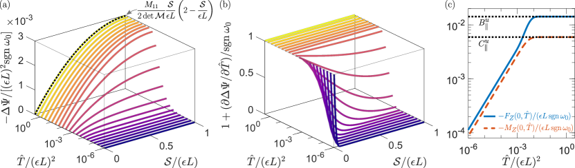
Figure 7: Axial rotation (twirling) in viscous fluid: viscous dynamics of a helical rod that is suddenly rotated at its base at a prescribed angular frequency, $\omega_{0}$ (here $\alpha^{u}=\pi/6$, $\nu=0$, $h=-1$ and $a/\lambda^{u}=10^{-2}$). We plot spatio-temporal diagrams of (a) the (negative) wavelength-averaged rotational displacement, $-\Delta\varPsi$; and (b) $1+(\partial\Delta\varPsi/\partial\hat{T})/\operatorname{sgn}\omega_{0}$, which corresponds to the leading-order angular velocity in the laboratory frame (normalised by $\omega_{0}$). In both panels, quantities are re-scaled according to the analytical solution (114). (c) Corresponding resultant force (solid curve) and moment (dashed curve) at the filament base from Eq. (115).

In Fig. 7a we use the solution (114) to construct a spatio-temporal diagram of the rotational displacement $\Delta\varPsi$: we plot curves of $\Delta\varPsi$ as a function of $\mathcal{S}$ for several different times $\hat{T}$ (the corresponding plot for $\Delta\mathcal{Z}$ is similar and will not be discussed here). Here we use typical parameter values for a bacteria flagellar filament in its normal left-handed helical form, i.e., $\alpha^{u}=\pi/6$, $\nu=0$, $h=-1$ and $a/\lambda^{u}=10^{-2}$ (Namba and Vonderviszt, 1997; Vogel and Stark, 2012; Son et al., 2013). We have re-scaled quantities according to Eq. (114): specifically, in Fig. 7a we plot $-\Delta\varPsi/[(\epsilon L)^{2}\operatorname{sgn}{\omega_{0}}]$ as a function of $\mathcal{S}/(\epsilon L)$ and $\hat{T}/(\epsilon L)^{2}$, so that the resulting curves are independent of the values of $\epsilon L$ and $\operatorname{sgn}{\omega_{0}}$. We observe an initial transient in which the displacement varies from zero, after which the solution approaches the quadratic profile (black dotted curve) predicted by the steady part of the solution, $\mathcal{Y}^{\mathrm{S}}$, in Eq. (114).

Figure 7b displays the corresponding spatio-temporal plot for $1+(\partial\Delta\varPsi/\partial\hat{T})/\operatorname{sgn}\omega_{0}$, which corresponds to the leading-order angular velocity (about the helix axis) in the laboratory frame, normalised by $\omega_{0}$: from Eqs. (103) and (105) (and using $\Delta\varPsi=\varPsi-2\pi h\mathcal{S}$), we have $1+(\partial\Delta\varPsi/\partial\hat{T})/\operatorname{sgn}\omega_{0}\sim\mathbf{e}_{z}\cdot(\omega_{0}\mathbf{e}_{z}+\boldsymbol{\omega})/\omega_{0}$. At early times, the bulk of the filament is evidently at rest relative to the fluid, with only a neighbourhood of the filament base (where the specified frequency is instantaneously applied for $\hat{T}>0$) rotating appreciably. The rotation rate propagates along the filament until the filament reaches a state of uniform rotation, which is approximately attained for times $\hat{T}/(\epsilon L)^{2}\gtrsim 10^{-2}$.

6.2.1 Resultant force and moment at the filament base

For locomotion driven by axial rotation of a helical filament in viscous fluid, a key quantity is the resultant force at the filament base, $F_{Z}(0,\hat{T})$: if the filament is no longer tethered but attached to a freely-swimming body, the swimming speed is determined by balancing this propulsive force with the total viscous drag on the body and filament (neglecting inertia). Thus, in absence of other forces, $F_{Z}(0,\hat{T})$ is proportional to the swimming velocity. The resultant moment $M_{Z}(0,\hat{T})$ corresponds to the torque required by the rotary motor to achieve the imposed frequency $\omega_{0}$.

Using the expressions for the linearised resultants $F_{Z}$ and $M_{Z}$ in terms of $\Delta\mathcal{Z}$ and $\Delta\varPsi$ (from combining Eq. (83) with the relations in Eq. (91)), we obtain, after simplifying,

$$-\frac{F_{Z}(0,\hat{T})}{\epsilon L\operatorname{sgn}\omega_{0}}=B_{\parallel}^{u}-\frac{8}{\pi^{2}}\sum_{n=0}^{\infty}\frac{1}{\left(2n+1\right)^{2}}\Bigg{\{} \frac{K_{2}^{u}-\mu_{-}B_{\parallel}^{u}}{\mu_{+}-\mu_{-}}\exp\left[-\frac{(2n+1)^{2}\pi^{2}}{4}\frac{\mu_{+}\hat{T}}{(\epsilon L)^{2}}\right]-\frac{K_{2}^{u}-\mu_{+}B_{\parallel}^{u}}{\mu_{+}-\mu_{-}}\exp\left[-\frac{(2n+1)^{2}\pi^{2}}{4}\frac{\mu_{-}\hat{T}}{(\epsilon L)^{2}}\right]\Bigg{\}},$$

$$-\frac{M_{Z}(0,\hat{T})}{\epsilon L\operatorname{sgn}\omega_{0}}=C_{\parallel}^{u}-\frac{8}{\pi^{2}}\sum_{n=0}^{\infty}\frac{1}{\left(2n+1\right)^{2}}\Bigg{\{} \frac{K_{4}^{u}-\mu_{-}C_{\parallel}^{u}}{\mu_{+}-\mu_{-}}\exp\left[-\frac{(2n+1)^{2}\pi^{2}}{4}\frac{\mu_{+}\hat{T}}{(\epsilon L)^{2}}\right]-\frac{K_{4}^{u}-\mu_{+}C_{\parallel}^{u}}{\mu_{+}-\mu_{-}}\exp\left[-\frac{(2n+1)^{2}\pi^{2}}{4}\frac{\mu_{-}\hat{T}}{(\epsilon L)^{2}}\right]\Bigg{\}}.$$ (115)

In Fig. 7c, we use these expressions to plot the corresponding resultant force and moment at the filament base for the solution shown in Figs. 7a–b. The figure shows how both resultants grow like $\hat{T}^{1/2}$ (i.e., diffusively) at early times. The resultants then approach the steady values (equal to the drag coefficients $B_{\parallel}^{u}$ and $C_{\parallel}^{u}$; black dotted lines) for times $\hat{T}/(\epsilon L)^{2}\gtrsim 10^{-2}$, corresponding to when the rotation rate is close to being spatially uniform (Fig. 7b).

7 Discussion and conclusions

7.1 Summary of findings

In this paper, we have studied slender, helical rods undergoing unsteady deformations in the presence of distributed forces and moments. Focussing on the case when the helix axis remains straight, we have derived an effective-column theory via an analytical reduction of the Kirchhoff rod equations. This analytical reduction is asymptotically valid in the limit of a highly-coiled filament, i.e., when the helical wavelength is much smaller than the typical deformation lengthscale. The (dimensionless) effective-column equations comprise two coupled PDEs, Eqs. (62)–(63), which correspond to wavelength-averaged force and moment balances about the helix axis; as well as two constraints on the external loading, Eq. (64), which state that a straight helix axis is only possible if the external force exactly balances the off-axis components of the filament acceleration, when averaged over the helical wavelength. Equations (62)–(63) can further be written as a quasi-linear system of equations, in terms of two independent variables that uniquely characterise the locally-helical shape. We focussed on two such pairs of variables in §4: the pitch angle and contour wavelength, and the wavelength-averaged longitudinal and rotational displacement.

The effective-column equations provide a simplified modelling framework, applicable to a wide variety of physical and biological settings, that allows for a great deal of analytical progress or rapid numerical solution. In particular, the equations account for unsteady displacements and rod inertia. In the absence of distributed loads, we demonstrated that the linearised equations reduce to the coupled wave equations previously proposed to describe the free vibrations of helical coil springs (Phillips and Costello, 1972; Jiang et al., 1989, 1991). Our analysis therefore provides a rigorous justification that the linearised stiffness coefficients can be applied locally (i.e., for each infinitesimal element) in situations involving unsteady deformations and distributed loads, provided that the loading is consistent with the assumption of a straight helix axis. In addition to the free vibrations of helical coil springs, we illustrated the applicability of our theory with two physical scenarios: (I) the compression/extension of helices under gravity (§5), and (II) the over-damped dynamics of helical rods twirling in viscous fluid (§6).

7.2 Discussion and outlook

Our effective-column description is distinct from classic perturbative approaches, which consider small deformations from a known base state, usually taken to be the undeformed helical shape (Goriely and Tabor, 1997a, b, c; Takano et al., 2003; Kim and Powers, 2005; Katsamba and Lauga, 2019). The main difference here is that we consider slowly-varying changes to an unknown leading-order shape. The relevant small parameter in our analysis is thus the gradient of the deformation along the arclength — there is no restriction on the global size of the displacements, provided that the (local) strains remain small. Our analysis is therefore similar to dimension reduction methods for slender structures (rods, plates, shells), which are based on the assumption that variations in the strains occur on lengthscales much larger than the cross-section dimensions of the structure. These methods systematically eliminate the dependence of field variables over the cross-section, to obtain a lower dimensional model describing an effective centreline or mid-surface (Lestringant and Audoly, 2020); examples include prismatic solids undergoing tensile necking (Audoly and Hutchinson, 2016), hyperelastic cylindrical membranes (Lestringant and Audoly, 2018; Yu and Fu, 2023), and elastic ribbons (Audoly and Neukirch, 2021; Kumar et al., 2023; Gomez et al., 2023). For the highly-coiled helical rods considered here, the effective centreline is simply the helix axis.

In addition, the multiple-scales analysis developed in §3 can be viewed as a homogenisation procedure in which the helical wavelength plays the role of a periodic unit cell over which the governing equations are averaged. In this sense, our analysis is similar to the work of Kehrbaum and Maddocks (2000) and Rey and Maddocks (2000) on straight rods with high intrinsic twist. However, in contrast to these studies, we did not pursue a Hamiltonian formulation of the Kirchhoff rod equations, but instead we worked directly with the equations of force and moment balance. This allowed us to readily incorporate general external forces and moments, including those that are non-conservative such as the hydrodynamic loading considered in §6. While simple hydrodynamic models such as resistive-force theory could be incorporated into a Hamiltonian formalism without much difficulty, we expect that the framework introduced here may more readily be extended to incorporate other, more complex, fluid frameworks, such as slender-body theory.

The basis of our asymptotic method is the helical solution of the inextensible Kirchhoff rod equations, in the case of a constant wrench aligned with the helix axis (Love, 1944); the assumptions of a highly-coiled helix and a straight helix axis then guarantee that this solution holds locally when distributed loads are present. Thus, we expect that our analysis can be extended to other situations, provided that there is sufficient symmetry such that a locally-helical solution persists. One important example is contact forces, either due to external radial confinement or self contact: under longitudinal compression, the helical symmetry guarantees that the net force arising from self-contact is directed towards the helix axis, i.e. along $-\mathbf{e}_{r}$, for which a locally-helical solution to the Kirchhoff rod equations still holds — see Chouaieb et al. (2006). Another example is the case of helical rods whose cross-section is rectangular (i.e., ribbons), which permit a helical solution in some cases (Goriely et al., 2001).

Physical significance of singularities

The analysis in §4.3 indicates that the steady effective-column equations may become singular, when the matrix of stiffness coefficients has zero determinant. In particular, in the $(\alpha,\Lambda)$ formulation of the dimensionless effective-column equations, these singularities can be visualised as branches of critical points on the $(\alpha,\Lambda)$ phase-plane; recall Fig. 3. As the system approaches one of these critical points, the magnitude of the gradient vector $(\partial\alpha/\partial\mathcal{S},\partial\Lambda/\partial\mathcal{S})$ tends to infinity — we observed such behaviour for compressive gravitational loading in §5 (see Fig. 5). However, as soon as the helix geometry varies on a lengthscale comparable to the helical wavelength, $S=O(1)$, the multiple-scales analysis presented in §3 will no longer be asymptotically valid. Nevertheless, we might expect that such critical points signal an underlying, physically-relevant instability in the steady system, whose description would require a detailed analysis of the rod equations on the wavelength lengthscale.

The behaviour of critical points as the undeformed pitch angle $\alpha^{u}$ varies (Fig. 3) has implications for their physical relevance. For small $\alpha^{u}$, the branches of critical points in Fig. 3 evidently lie at values of $\alpha$ much larger than the undeformed value $\alpha^{u}$ (drawn as circles in Fig. 3). Hence, in the vicinity of the critical points, we expect that the filament will be under a large amount of longitudinal compression (i.e., the force resultant $F_{Z}<0$) as it must be compressed to a pitch angle $\alpha>\alpha^{u}$. For given external loads, as $\mathcal{S}$ varies and the system moves through the $(\alpha,\Lambda)$ phase plane, we therefore expect that the helix axis buckles before the system is able to approach the vicinity of any critical point (neglecting dynamic effects); we discussed this point in the context of gravitational loading in §5. However, for larger values of $\alpha^{u}$, the branch closest to the undeformed point $(\alpha^{u},1)$ lies at values $\alpha<\alpha^{u}$ where the filament is under longitudinal tension ($F_{Z}>0$). It is therefore conceivable that the system remains stable as it approaches such critical points, which may correspond to tensile instabilities that can be observed experimentally.

To further illustrate this behaviour, we show in Fig. 8 contour plots of the dimensionless force resultant $F_{Z}$ (top panels) and moment resultant $M_{Z}$ (bottom panels) for three different values of $\alpha^{u}$ in the physical range $0<\alpha<\pi/2$ (these resultants are evaluated using Eq. (66)). For the smallest value $\alpha^{u}=\pi/6$ (left column), the critical branches $\Lambda_{\pm}$ (black curves) both lie to the right of the zero-force contour $F_{Z}=0$ (red dashed curve), where $F_{Z}<0$. For $\alpha^{u}\gtrsim\pi/3$, however, the branch closest to the undeformed point $(\alpha^{u},1)$ instead lies in the region $F_{Z}>0$; see the middle and right columns in Fig. 8. We also observe that the critical branch lies in the region $M_{Z}/h<0$.

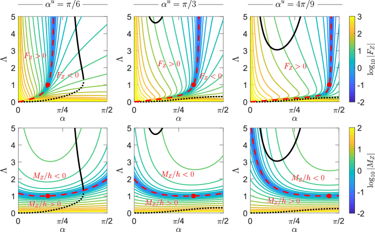
Figure 8: Contour plots of the dimensionless resultant force $F_{Z}$ (top panels) and moment $M_{Z}$ (bottom panels) on the $(\alpha,\Lambda)$-plane, coloured according to the logarithm of their magnitude (see colourbars; here $\nu=1/3$). In each plot, the zero contour separating regions of positive and negative force/moment resultant is shown (red dashed curves); this contour passes through the undeformed point $(\alpha,\Lambda)=(\alpha^{u},1)$ (red circles). Also shown are the roots $\Lambda_{-}$ and $\Lambda_{+}$ (solid and dotted black curves, respectively) from Eq. (78), at which the matrix of stiffness coefficients is singular.

The above discussion indicates that tensile instabilities are a generic phenomenon when helical rods are subject to both distributed forces and moments. Indeed, instabilities characterised by large stretching deformations (with approximately straight helix axis) have been observed in several systems. Examples include the abrupt, localised uncoiling of microscopic helical ribbons under directed fluid flow (Pham et al., 2015); and helices composed of magneto-rheological elastomers (MREs), which suddenly extend from a highly-collapsed state (attained due to long range dipole-dipole interactions) as the gradient of the magnetic field exceeds a critical value (Sano et al., 2022). It remains an intriguing possibility if these instabilities can be predicted using the analytical framework developed here.

Axis bending

Finally, our analysis rests on a number of assumptions (summarised earlier in §1.2), the most severe of which is that the helix axis remains straight. Indeed, the constraints in (64) place a strong restriction on what external forces are consistent with this assumption. If the helix axis is not assumed straight, it is expected to bend over the deformation lengthscale $[s]=(B/[f])^{1/3}$, which arises from a balance between the external force density $[f]$ and the typical force (per unit length) required to bend the filament; recall the discussion in §2.5. In dimensionless variables, this introduces a bending lengthscale, $\mathscr{S}$, defined by $S=\epsilon^{-1/3}\mathscr{S}$ (using $S=s/\lambda^{u}$ and $\epsilon=(\lambda^{u}/[s])^{3}$). It is then necessary to generalise the locally-helical solution in §3.2 to incorporate a slowly-varying isometry $Q=Q(\mathscr{S},T)$ applied to the leading-order directors. The resulting bending strains, resulting from $\mathscr{S}$-derivatives of $Q$, would contribute $\operatorname{ord}(\epsilon^{1/3})$ terms to the strain components, meaning that a regular asymptotic expansion in $\epsilon$ (like that in §3.3) is no longer appropriate. This additional complexity is the topic of future work, which aims to obtain an effective-beam model describing the geometrically-nonlinear displacements of a helical rod in three dimensions. Such a model would have immediate applications in a number of contexts. For example, when combined with mechanical modelling of polymorphic shapes (Srigiriraju and Powers, 2005), it would allow the full dynamics of flagellar filaments on swimming bacteria to be modelled (Turner et al., 2000). Other potential biomechanical applications include the dynamics of flicking for bacteria (Xie et al., 2011; Son et al., 2013), bacterial pumps (Gao et al., 2015) and artificial flagella (Zhang et al., 2010; Huang et al., 2019).

Appendix AppendixA Leading-order centreline and winding angle associated with the locally-helical ansatz

In this Appendix we calculate the leading-order centreline, $\mathbf{R}^{(0)}$, and winding angle, $\Psi$, associated with our ansatz of a locally-helical shape. From Eqs. (28) and (31), the unit tangent vector $\mathbf{d}_{3}^{(0)}=h\sin\alpha\,\mathbf{e}_{\theta}+\cos\alpha\,\mathbf{e}_{z}$. Substituting into the inextensibility constraint (14) and expanding the derivative using the chain rule (27), we obtain

$$\frac{\partial\mathbf{R}^{(0)}}{\partial S}\bigg{\lvert}_{\mathcal{S}}+\epsilon\frac{\partial\mathbf{R}^{(0)}}{\partial\mathcal{S}}\bigg{\lvert}_{S}=h\sin\alpha\,\mathbf{e}_{\theta}+\cos\alpha\,\mathbf{e}_{z}.$$ (116)

We express $\mathbf{R}^{(0)}$ in terms of components perpendicular and parallel to the helix axis:

$$\mathbf{R}^{(0)}(S,\mathcal{S},T)={\mathbf{R}^{(0)}}^{\perp}(S,\mathcal{S},T)+Z^{(0)}(S,\mathcal{S},T)\,\mathbf{e}_{z}\qquad\mathrm{where}\qquad\mathbf{e}_{z}\cdot{\mathbf{R}^{(0)}}^{\perp}=0.$$ (117)

Inserting into Eq. (116) gives

$$\frac{\partial{\mathbf{R}^{(0)}}^{\perp}}{\partial S}\bigg{\lvert}_{\mathcal{S}}+\epsilon\frac{\partial{\mathbf{R}^{(0)}}^{\perp}}{\partial\mathcal{S}}\bigg{\lvert}_{S}=h\sin\alpha\,\mathbf{e}_{\theta},\quad\frac{\partial Z^{(0)}}{\partial S}\bigg{\lvert}_{\mathcal{S}}+\epsilon\frac{\partial Z^{(0)}}{\partial\mathcal{S}}\bigg{\lvert}_{S}=\cos\alpha.$$ (118)

Due to both $S$ and $\mathcal{S}$ derivatives, it is not immediately clear how to integrate the equations in Eq. (118). Consider first the equation for the longitudinal coordinate, $Z^{(0)}$. Physically, we expect that $Z^{(0)}$ consists of its average value over the wavelength centred at $\mathcal{S}$, of size comparable to the total contour length, $L=O(\epsilon^{-1})$, together with an $O(1)$ part that has zero average. Seeking a solution in his form, we obtain

$$Z^{(0)}(S,\mathcal{S},T)\sim\epsilon^{-1}\mathcal{Z}(\mathcal{S},T)+\Delta S\cos\alpha(\mathcal{S},T)\qquad\mathrm{where}\qquad\frac{\partial\mathcal{Z}}{\partial\mathcal{S}}\bigg{\lvert}_{S}=\cos\alpha.$$ (119)

It may be verified that this satisfies Eq. (118) to leading order, i.e., up to terms of size $O(\epsilon)$, using

$$\Delta S=S-\epsilon^{-1}\mathcal{S}=O(1),\quad\frac{\partial(\Delta S)}{\partial S}\bigg{\lvert}_{\mathcal{S}}=1,\quad\frac{\partial(\Delta S)}{\partial\mathcal{S}}\bigg{\lvert}_{S}=-\epsilon^{-1},$$

For the transverse displacement, we seek a solution in the form

$${\mathbf{R}^{(0)}}^{\perp}(S,\mathcal{S},T)=\mathcal{R}(\mathcal{S},T)\mathbf{e}_{r}(S,\mathcal{S},T),$$

where $\mathcal{R}=\Lambda\sin\alpha/(2\pi)$ is the slowly-varying helical radius. Using $\partial\mathbf{e}_{r}/\partial S\lvert_{\mathcal{S}}=[\partial\Psi/\partial S\lvert_{\mathcal{S}}]\mathbf{e}_{\theta}$ and $\partial\mathbf{e}_{r}/\partial\mathcal{S}\lvert_{S}=[\partial\Psi/\partial\mathcal{S}\lvert_{S}]\mathbf{e}_{\theta}$ (which follow from Eq. (29)), Eq. (118) becomes, upon neglecting terms of $O(\epsilon)$,

$$\frac{\partial\Psi}{\partial S}\bigg{\lvert}_{\mathcal{S}}+\epsilon\frac{\partial\Psi}{\partial\mathcal{S}}\bigg{\lvert}_{S}\sim\frac{2\pi h}{\Lambda}.$$

Similar to the equation for $Z^{(0)}$, the solution is

$$\Psi(S,\mathcal{S},T)\sim\epsilon^{-1}\varPsi(\mathcal{S},T)+\frac{2\pi h\Delta S}{\Lambda(\mathcal{S},T)}\qquad\mathrm{where}\qquad\frac{\partial\varPsi}{\partial\mathcal{S}}\bigg{\lvert}_{S}=\frac{2\pi h}{\Lambda}.$$ (120)

Physically, $\mathcal{Z}$ and $\varPsi$ correspond to the wavelength-averaged longitudinal coordinate and winding angle, respectively; their slow derivatives, $\partial\mathcal{Z}/\partial\mathcal{S}\lvert_{S}$ and $\partial\varPsi/\partial\mathcal{S}\lvert_{S}$, can be interpreted as extensional and twist strains of the effective column. The boundary condition at the filament base, Eq. (23), implies that $\mathcal{Z}(0,T)=\varPsi(0,T)=0$; from Eqs. (119)–(120), we then obtain expressions for $\mathcal{Z}$ and $\varPsi$ in terms $\alpha$ and $\Lambda$:

$$\mathcal{Z}(\mathcal{S},T)=\int_{0}^{\mathcal{S}}\cos\alpha(\xi,T)\,\mathrm{d}\xi,\quad\varPsi(\mathcal{S},T)=2\pi h\int_{0}^{\mathcal{S}}\frac{\mathrm{d}\xi}{\Lambda(\xi,T)}.$$

Combining with the above solutions for $Z^{(0)}$ and ${\mathbf{R}^{(0)}}^{\perp}$ yields the expressions reported in the main text (Eqs. (32)–(34)).

Appendix AppendixB Solvability conditions for the first-order problem using the Fredholm Alternative Theorem

In this Appendix, we apply the Fredholm Alternative Theorem to the first-order problem obtained in §3.5 of the main text. We systematically derive solvability conditions that are equivalent to those obtained by direct averaging.

AppendixB.1 Component form of the first-order problem

It is convenient to express vectors as a matrix of components (referred to as a triple) with respect to the leading-order directors $\{\mathbf{d}_{1}^{(0)},\mathbf{d}_{2}^{(0)},\mathbf{d}_{3}^{(0)}\}$; a similar strategy was employed by Goriely and Tabor (1997c) to obtain dispersion relations for small-amplitude oscillations of helical rods. To avoid ambiguity in what follows, we use the convention that sans serif fonts denote a matrix of components. Using the expressions in Eqs. (28), (31), (41) and (47), the triples corresponding to the unit vectors $\mathbf{e}_{r}$, $\mathbf{e}_{\theta}$, $\mathbf{e}_{z}$, tangent vector $\mathbf{d}_{3}^{(0)}=\mathbf{t}$, strain vector $\mathbf{U}^{(0)}$, resultant moment $\mathbf{M}^{(0)}$ and resultant force $\mathbf{F}^{(0)}$ are, respectively,

$$\mathsf{e}_{r}=\begin{pmatrix}-1\\ 0\\ 0\end{pmatrix},\quad\mathsf{e}_{\theta}=\begin{pmatrix}0\\ -\cos\alpha\\ h\sin\alpha\end{pmatrix},\quad\mathsf{e}_{z}=\begin{pmatrix}0\\ h\sin\alpha\\ \cos\alpha\end{pmatrix},\quad\mathsf{d}_{3}^{(0)}=\begin{pmatrix}0\\ 0\\ 1\end{pmatrix},\quad\mathsf{U}^{(0)}=\begin{pmatrix}0\\ \mathcal{K}\\ \mathcal{T}\end{pmatrix},\quad\mathsf{M}^{(0)}=\mathcal{R}F_{Z}\mathsf{e}_{\theta}+M_{Z}\mathsf{e}_{z},\quad\mathsf{F}^{(0)}=F_{Z}\mathsf{e}_{z}.$$ (121)

We define the triples $\mathsf{\tilde{U}}^{(1)}$, $\mathsf{\tilde{M}}^{(1)}$, $\mathsf{\tilde{F}}^{(1)}$ as the components of $\mathbf{U}^{(1)}$, $\mathbf{M}^{(1)}$, $\mathbf{F}^{(1)}$ that are independent of $\boldsymbol{\Phi}$ (recall the identity in Eq. (39)). Explicitly,

$$\mathsf{\tilde{U}}^{(1)}=\begin{pmatrix}U_{1}^{(1)}\\ U_{2}^{(1)}\\ U_{3}^{(1)}\end{pmatrix},\quad\mathsf{\tilde{M}}^{(1)}=\begin{pmatrix}M_{1}^{(1)}\\ M_{2}^{(1)}\\ M_{3}^{(1)}\end{pmatrix},\quad\mathsf{\tilde{F}}^{(1)}=\begin{pmatrix}F_{1}^{(1)}\\ F_{2}^{(1)}\\ F_{3}^{(1)}\end{pmatrix}.$$

We also write $\mathsf{\Phi}$, $\mathsf{\Theta}$, $\mathsf{M}_{e}^{(0)}$, $\mathsf{F}_{e}^{(0)}$ and $\mathsf{R}^{(0)}$ for the triples corresponding to, respectively, $\boldsymbol{\Phi}$, $\boldsymbol{\Theta}$, $\mathbf{M}_{e}^{(0)}$, $\mathbf{F}_{e}^{(0)}$ and $\mathbf{R}^{(0)}$. The first-order problem, consisting of Eqs. (51) and (54)–(56), can then be expressed as

$$\frac{\partial\mathsf{\Phi}}{\partial S}\bigg{\lvert}_{\mathcal{S}}+\mathsf{U}^{(0)}\times\mathsf{\Phi}-\mathsf{\tilde{U}}^{(1)}+\mathsf{\Theta}=\mathsf{0}_{3\times 1},$$

$$\frac{\partial\mathsf{\tilde{M}}^{(1)}}{\partial S}\bigg{\lvert}_{\mathcal{S}}+\mathsf{U}^{(0)}\times\mathsf{\tilde{M}}^{(1)}+\mathsf{\tilde{U}}^{(1)}\times\mathsf{M}^{(0)}+\mathsf{d}_{3}^{(0)}\times\mathsf{\tilde{F}}^{(1)}=-\frac{\partial\mathsf{M}^{(0)}}{\partial\mathcal{S}}\bigg{\lvert}_{S}-\delta\mathsf{M}_{e}^{(0)},$$

$$\frac{\partial\mathsf{\tilde{F}}^{(1)}}{\partial S}\bigg{\lvert}_{\mathcal{S}}+\mathsf{U}^{(0)}\times\mathsf{\tilde{F}}^{(1)}+\mathsf{\tilde{U}}^{(1)}\times\mathsf{F}^{(0)}=-\frac{\partial\mathsf{F}^{(0)}}{\partial\mathcal{S}}\bigg{\lvert}_{S}-\mathsf{F}_{e}^{(0)}+\epsilon\frac{\partial^{2}\mathsf{R}^{(0)}}{\partial T^{2}},\qquad\mathsf{\tilde{M}}^{(1)}=\mathsf{K}_{\nu}\mathsf{\tilde{U}}^{(1)},$$ (122)

where, in the final equation, we introduce the diagonal stiffness matrix $\mathsf{K}_{\nu}=\operatorname{diag}{(1,1,1/[1+\nu])}$.

We eliminate $\mathsf{\tilde{U}}^{(1)}$ using the final equation in (122). The remaining equations in (122) can then be written as the linear system

$$\frac{\partial\mathsf{Y}^{(1)}}{\partial S}\bigg{\lvert}_{\mathcal{S}}+\mathsf{A}\,\mathsf{Y}^{(1)}=\begin{pmatrix}-\mathsf{\Theta}\\ -\partial\mathsf{M}^{(0)}/\partial\mathcal{S}\lvert_{S}-\delta\mathsf{M}_{e}^{(0)}\\ -\partial\mathsf{F}^{(0)}/\partial\mathcal{S}\lvert_{S}-\mathsf{F}_{e}^{(0)}+\epsilon\,\partial^{2}\mathsf{R}^{(0)}/\partial T^{2}\end{pmatrix},$$ (123)

where we have introduced the nine-dimensional solution vector $\mathsf{Y}^{(1)}$ and the $9\times 9$ block matrix $\mathsf{A}$:

$$\mathsf{Y}^{(1)}=\begin{pmatrix}\mathsf{\Phi}\\ \mathsf{\tilde{M}}^{(1)}\\ \mathsf{\tilde{F}}^{(1)}\end{pmatrix},\quad\mathsf{A}=\begin{pmatrix}\left[\mathsf{U}^{(0)}\right]_{\times}&-\mathsf{K}_{\nu}^{-1}&\mathsf{0}_{3\times 3}\\ \mathsf{0}_{3\times 3}&\left[\mathsf{U}^{(0)}\right]_{\times}-\left[\mathsf{M}^{(0)}\right]_{\times}\mathsf{K}_{\nu}^{-1}&\left[\mathsf{d}_{3}^{(0)}\right]_{\times}\\ \mathsf{0}_{3\times 3}&-\left[\mathsf{F}^{(0)}\right]_{\times}\mathsf{K}_{\nu}^{-1}&\left[\mathsf{U}^{(0)}\right]_{\times}\end{pmatrix}.$$

Here we use the notation $\left[\mathsf{V}\right]_{\times}$ for the $3\times 3$ skew-symmetric matrix whose off-diagonal elements are the components of the triple $\mathsf{V}$, so that for any triples $\mathsf{V}$, $\mathsf{W}$ we have the identity $\left[\mathsf{V}\right]_{\times}\mathsf{W}=\mathsf{V}\times\mathsf{W}$.

AppendixB.2 Homogeneous adjoint problem

To formulate solvability conditions on the first-order problem, we consider the homogeneous adjoint problem associated with Eq. (123). In component form, with solution vector $\mathsf{Y}^{*}$, this reads

$$-\frac{\partial\mathsf{Y}^{*}}{\partial S}\bigg{\lvert}_{\mathcal{S}}+\mathsf{A}^{\mathrm{T}}\mathsf{Y}^{*}=\mathsf{0}_{9\times 1}.$$ (124)

Using skew-symmetry of the matrix blocks, we calculate

$$\mathsf{A}^{\mathrm{T}}=-\begin{pmatrix}\left[\mathsf{U}^{(0)}\right]_{\times}&\mathsf{0}_{3\times 3}&\mathsf{0}_{3\times 3}\\ \mathsf{K}_{\nu}^{-1}&\left[\mathsf{U}^{(0)}\right]_{\times}-\mathsf{K}_{\nu}^{-1}\left[\mathsf{M}^{(0)}\right]_{\times}&-\mathsf{K}_{\nu}^{-1}\left[\mathsf{F}^{(0)}\right]_{\times}\\ \mathsf{0}_{3\times 3}&\left[\mathsf{d}_{3}^{(0)}\right]_{\times}&\left[\mathsf{U}^{(0)}\right]_{\times}\end{pmatrix}.$$

Writing $\mathsf{Y}^{*}=(\mathsf{\Phi}^{*},\mathsf{M}^{*},\mathsf{F}^{*})^{\mathrm{T}}$, the homogeneous adjoint problem can be written as

$$\frac{\partial\mathsf{\Phi}^{*}}{\partial S}\bigg{\lvert}_{\mathcal{S}}+\mathsf{U}^{(0)}\times\mathsf{\Phi}^{*}=\mathsf{0}_{3\times 1},$$

$$\frac{\partial\mathsf{M}^{*}}{\partial S}\bigg{\lvert}_{\mathcal{S}}+\mathsf{U}^{(0)}\times\mathsf{M}^{*}+\mathsf{K}_{\nu}^{-1}\left(\mathsf{\Phi}^{*}-\mathsf{M}^{(0)}\times\mathsf{M}^{*}-\mathsf{F}^{(0)}\times\mathsf{F}^{*}\right)=\mathsf{0}_{3\times 1},$$

$$\frac{\partial\mathsf{F}^{*}}{\partial S}\bigg{\lvert}_{\mathcal{S}}+\mathsf{U}^{(0)}\times\mathsf{F}^{*}+\mathsf{d}_{3}^{(0)}\times\mathsf{M}^{*}=\mathsf{0}_{3\times 1}.$$ (125)

Without the $\mathsf{K}_{\nu}^{-1}$ term, the second and third equations in (125) are equivalent to the leading-order force and moment balances (Eqs. (43)–(44)) when the force and moment resultants are swapped, i.e., with $\mathsf{M}^{*}=\mathsf{F}^{(0)}$ and $\mathsf{F}^{*}=\mathsf{M}^{(0)}$. We also note that the first equation is trivially satisfied by $\mathsf{\Phi}^{*}=\mathsf{0}_{3\times 1}$. Hence, seeking solutions for which $\mathsf{\Phi}^{*}=\mathsf{0}_{3\times 1}$ and $\mathsf{M}^{(0)}\times\mathsf{M}^{*}+\mathsf{F}^{(0)}\times\mathsf{F}^{*}=\mathsf{0}_{3\times 1}$ (which ensures that the $\mathsf{K}_{\nu}^{-1}$ term is zero), we obtain two linearly independent solutions:

$$\mathsf{\Phi}^{*}=\mathsf{0}_{3\times 1},\quad\mathsf{M}^{*}=\mathsf{0}_{3\times 1},\quad\mathsf{F}^{*}=\mathsf{F}^{(0)}\qquad\mathrm{and}\qquad\mathsf{\Phi}^{*}=\mathsf{0}_{3\times 1},\quad\mathsf{M}^{*}=\mathsf{F}^{(0)},\quad\mathsf{F}^{*}=\mathsf{M}^{(0)}.$$

Substituting for $\mathsf{F}^{(0)}$ and $\mathsf{M}^{(0)}$ using the expressions in Eq. (121) and re-scaling, we have the linearly independent solutions for $\mathsf{Y}^{*}$:

$$\mathsf{Y}^{*}_{1}=\begin{pmatrix}\mathsf{0}_{3\times 1}\\ \mathsf{0}_{3\times 1}\\ \mathsf{e}_{z}\end{pmatrix},\quad\mathsf{Y}^{*}_{2}=\begin{pmatrix}\mathsf{0}_{3\times 1}\\ \mathsf{e}_{z}\\ \mathcal{R}\mathsf{e}_{\theta}\end{pmatrix},$$ (126)

where, in the second solution, we have taken a linear combination to remove the $\mathsf{e}_{z}$-component of $\mathsf{M}^{(0)}$. Since these solutions are independent of $S$, they must correspond to eigenvectors of $\mathsf{A}^{\mathrm{T}}$ with eigenvalue zero, as can be readily verified directly.

To find other solutions to Eq. (125), we note that if $\mathsf{M}^{*}=\mathsf{0}_{3\times 1}$ the second equation in (125) simplifies to

$$\mathsf{\Phi}^{*}-\mathsf{F}^{(0)}\times\mathsf{F}^{*}=\mathsf{0}_{3\times 1}.$$

With $\mathsf{M}^{*}=\mathsf{0}_{3\times 1}$, the other equations in (125) are equivalent to the statement that $\mathsf{\Phi}^{*}$ and $\mathsf{F}^{*}$ are triples corresponding to constant vectors, and so they must be a linear combination of the Cartesian unit vectors $\mathsf{e}_{x}$, $\mathsf{e}_{y}$ and $\mathsf{e}_{z}$. Using Eqs. (29) and (121), we have

$$\mathsf{e}_{x}=\cos\Psi\mathsf{e}_{r}-\sin\Psi\mathsf{e}_{\theta}=\begin{pmatrix}-\cos\Psi\\ \cos\alpha\sin\Psi\\ -h\sin\alpha\sin\Psi\end{pmatrix},\quad\mathsf{e}_{y}=\sin\Psi\mathsf{e}_{r}+\cos\Psi\mathsf{e}_{\theta}=\begin{pmatrix}-\sin\Psi\\ -\cos\alpha\cos\Psi\\ h\sin\alpha\cos\Psi\end{pmatrix}.$$

We can therefore generate linearly independent solutions of the form $\mathsf{Y}^{*}=(\mathsf{F}^{(0)}\times\mathsf{F}^{*},\mathsf{0}_{3\times 1},\mathsf{F}^{*})^{\mathrm{T}}$ by choosing $\mathsf{F}^{*}=\mathsf{e}_{x}$, $\mathsf{F}^{*}=\mathsf{e}_{y}$ and $\mathsf{F}^{*}=\mathsf{e}_{z}$. The choice $\mathsf{F}^{*}=\mathsf{e}_{z}$ yields $\mathsf{Y}^{*}_{1}$ above, while choosing $\mathsf{F}^{*}=\mathsf{e}_{x}$ and $\mathsf{F}^{*}=\mathsf{e}_{y}$ yields

$$\mathsf{Y}^{*}_{3}=\begin{pmatrix}F_{Z}\mathsf{e}_{y}\\ \mathsf{0}_{3\times 1}\\ \mathsf{e}_{x}\end{pmatrix},\quad\mathsf{Y}^{*}_{4}=\begin{pmatrix}-F_{Z}\mathsf{e}_{x}\\ \mathsf{0}_{3\times 1}\\ \mathsf{e}_{y}\end{pmatrix}.$$ (127)

These solutions can also be derived by considering the eigenvectors of $\mathsf{A}^{\mathrm{T}}$ with eigenvalue $\pm 2\pi i/\Lambda$; these eigenvalues arise as the non-zero eigenvalues of the $\left[\mathsf{U}^{(0)}\right]_{\times}$ blocks on the diagonal of $\mathsf{A}^{\mathrm{T}}$.

Other linearly independent solutions of Eq. (125) can be determined from the remaining eigenvalues and eigenvectors of $\mathsf{A}^{\mathrm{T}}$. The other eigenvalues generally have a non-zero real part and an imaginary part that is not equal to $\pm 2\pi/\Lambda$. This is a consequence of the $\mathsf{K}_{\nu}^{-1}$ terms in $\mathsf{A}$, which makes the first-order operator different to that obtained in the leading-order problem. Since these solutions are not $\Lambda$-periodic, they are not relevant in determining solvability conditions so we do not discuss them here.

AppendixB.3 Solvability conditions

We are now in a position to formulate the solvability conditions for the first-order problem (123). Dotting Eq. (123) with $\mathsf{Y}^{*}_{i}$ and integrating by parts over the wavelength centred at $S=\epsilon^{-1}\mathcal{S}$, we obtain ($i=1,2,3,4$)

$$\int_{\epsilon^{-1}\mathcal{S}-\Lambda/2}^{\epsilon^{-1}\mathcal{S}+\Lambda/2}\mathsf{Y}^{*}_{i}\cdot\begin{pmatrix}-\mathsf{\Theta}\\ -\partial\mathsf{M}^{(0)}/\partial\mathcal{S}\lvert_{S}-\delta\mathsf{M}_{e}^{(0)}\\ -\partial\mathsf{F}^{(0)}/\partial\mathcal{S}\lvert_{S}-\mathsf{F}_{e}^{(0)}+\epsilon\,\partial^{2}\mathsf{R}^{(0)}/\partial T^{2}\end{pmatrix}\mathrm{d}S =\int_{\epsilon^{-1}\mathcal{S}-\Lambda/2}^{\epsilon^{-1}\mathcal{S}+\Lambda/2}\mathsf{Y}^{*}_{i}\cdot\left(\frac{\partial\mathsf{Y}^{(1)}}{\partial S}\bigg{\lvert}_{\mathcal{S}}+\mathsf{A}\,\mathsf{Y}^{(1)}\right)\mathrm{d}S$$

$$=\left[\mathsf{Y}^{*}_{i}\cdot\mathsf{Y}^{(1)}\right]_{\epsilon^{-1}\mathcal{S}-\Lambda/2}^{\epsilon^{-1}\mathcal{S}+\Lambda/2}+\int_{\epsilon^{-1}\mathcal{S}-\Lambda/2}^{\epsilon^{-1}\mathcal{S}+\Lambda/2}\mathsf{Y}^{(1)}\cdot\left(-\frac{\partial\mathsf{Y}^{*}_{i}}{\partial S}\bigg{\lvert}_{\mathcal{S}}+\mathsf{A}^{\mathrm{T}}\mathsf{Y}^{*}_{i}\right)\mathrm{d}S.$$

The final integral disappears by definition of the adjoint solution, $\mathsf{Y}^{*}_{i}$. Requiring that $\mathsf{Y}^{(1)}$ is $\Lambda$-periodic, the boundary terms on the right-hand side also vanish and we are left with

$$\int_{\epsilon^{-1}\mathcal{S}-\Lambda/2}^{\epsilon^{-1}\mathcal{S}+\Lambda/2}\mathsf{Y}^{*}_{i}\cdot\begin{pmatrix}-\mathsf{\Theta}\\ -\partial\mathsf{M}^{(0)}/\partial\mathcal{S}\lvert_{S}-\delta\mathsf{M}_{e}^{(0)}\\ -\partial\mathsf{F}^{(0)}/\partial\mathcal{S}\lvert_{S}-\mathsf{F}_{e}^{(0)}+\epsilon\,\partial^{2}\mathsf{R}^{(0)}/\partial T^{2}\end{pmatrix}\mathrm{d}S=0.$$ (128)

Inserting the first two homogeneous adjoint solutions $\mathsf{Y}^{*}_{1}$ and $\mathsf{Y}^{*}_{2}$ (Eq. (126)) into Eq. (128), and using the fact that the triples $\mathsf{e}_{\theta}$, $\mathsf{e}_{z}$, $\mathsf{F}^{(0)}$ and $\mathsf{M}^{(0)}$ and the radius $\mathcal{R}$ are independent of $S$, we obtain the solvability conditions

$$-\overline{\mathsf{e}_{z}\cdot\frac{\partial\mathsf{F}^{(0)}}{\partial\mathcal{S}}\bigg{\lvert}_{S}}-\overline{\mathsf{e}_{z}\cdot\mathsf{F}_{e}^{(0)}}+\overline{\mathsf{e}_{z}\cdot\epsilon\frac{\partial^{2}\mathsf{R}^{(0)}}{\partial T^{2}}}=0,$$

$$-\overline{\mathsf{e}_{z}\cdot\frac{\partial\mathsf{M}^{(0)}}{\partial\mathcal{S}}\bigg{\lvert}_{S}}-\delta\overline{\mathsf{e}_{z}\cdot\mathsf{M}_{e}^{(0)}}-\mathcal{R}\overline{\mathsf{e}_{\theta}\cdot\frac{\partial\mathsf{F}^{(0)}}{\partial\mathcal{S}}\bigg{\lvert}_{S}}-\mathcal{R}\overline{\mathsf{e}_{\theta}\cdot\mathsf{F}_{e}^{(0)}}+\mathcal{R}\overline{\mathsf{e}_{\theta}\cdot\epsilon\frac{\partial^{2}\mathsf{R}^{(0)}}{\partial T^{2}}}=0,$$

where here, as in the main text, we use bars to denote the average over the helical wavelength. When written back in vector form, these solvability conditions are equivalent to Eqs. (58)–(59) in the main text.

For the other two solvability conditions, we first note from the expression for $\boldsymbol{\Theta}$ in Eq. (50) that the off-axis components of the triple $\mathsf{\Theta}$ are also independent of $S$, so that $\overline{\mathsf{e}_{x}\cdot\mathsf{\Theta}}=\overline{\mathsf{e}_{y}\cdot\mathsf{\Theta}}=0$ (since $\overline{\mathsf{e}_{x}\cdot\mathsf{e}_{r}}=\overline{\cos\Psi}=0$ and $\overline{\mathsf{e}_{y}\cdot\mathsf{e}_{r}}=\overline{\sin\Psi}=0$). Substituting the homogeneous adjoint solutions with $i=3,4$ (Eq. (127)) into Eq. (128), the corresponding solvability conditions then reduce to

$$-\overline{\mathsf{e}_{x}\cdot\frac{\partial\mathsf{F}^{(0)}}{\partial\mathcal{S}}\bigg{\lvert}_{S}}-\overline{\mathsf{e}_{x}\cdot\mathsf{F}_{e}^{(0)}}+\overline{\mathsf{e}_{x}\cdot\epsilon\frac{\partial^{2}\mathsf{R}^{(0)}}{\partial T^{2}}}=0,\quad-\overline{\mathsf{e}_{y}\cdot\frac{\partial\mathsf{F}^{(0)}}{\partial\mathcal{S}}\bigg{\lvert}_{S}}-\overline{\mathsf{e}_{y}\cdot\mathsf{F}_{e}^{(0)}}+\overline{\mathsf{e}_{y}\cdot\epsilon\frac{\partial^{2}\mathsf{R}^{(0)}}{\partial T^{2}}}=0.$$

In vector form, these are equivalent to the solvability conditions in Eq. (61).

Appendix AppendixC Effective-column equations in terms of Frenet curvature and torsion

From Eq. (42), we have $\Lambda=2\pi/\sqrt{\mathcal{K}^{2}+\mathcal{T}^{2}}$, $\cos\alpha=h\mathcal{T}/\sqrt{\mathcal{K}^{2}+\mathcal{T}^{2}}$ and $\sin\alpha=\mathcal{K}/\sqrt{\mathcal{K}^{2}+\mathcal{T}^{2}}$. The leading-order moment and force resultants, $M_{Z}$ and $F_{Z}$ (defined in Eq. (48)), and the slowly-varying helical radius, $\mathcal{R}$ (defined in Eq. (34)), can then be written in terms of $(\mathcal{K},\mathcal{T})$ alone:

$$M_{Z}=\frac{h}{\sqrt{\mathcal{K}^{2}+\mathcal{T}^{2}}}\left[\mathcal{K}\left(\mathcal{K}-\mathcal{K}^{u}\right)+\mathcal{T}\frac{\mathcal{T}-\mathcal{T}^{u}}{1+\nu}\right],\quad F_{Z}=h\sqrt{\mathcal{K}^{2}+\mathcal{T}^{2}}\left[\frac{\mathcal{T}-\mathcal{T}^{u}}{1+\nu}-\mathcal{T}\frac{\mathcal{K}-\mathcal{K}^{u}}{\mathcal{K}}\right],\quad\mathcal{R}=\frac{\mathcal{K}}{\mathcal{K}^{2}+\mathcal{T}^{2}}.$$

The effective-column equations (62)–(63) yield the first-order system for $\mathcal{K}(\mathcal{S},T)$ and $\mathcal{T}(\mathcal{S},T)$:

$$\mathcal{C}_{1}\frac{\partial\mathcal{T}}{\partial\mathcal{S}}+\mathcal{C}_{2}\frac{\partial\mathcal{K}}{\partial\mathcal{S}}+\overline{\mathbf{e}_{z}\cdot\mathbf{F}_{e}^{(0)}}-h\frac{\partial^{2}}{\partial T^{2}}\left(\int_{0}^{\mathcal{S}}\frac{\mathcal{T}}{\sqrt{\mathcal{K}^{2}+\mathcal{T}^{2}}}\Bigg{\lvert}_{\mathcal{S}=\xi}\mathrm{d}\xi\right)=0,$$

$$\mathcal{C}_{3}\frac{\partial\mathcal{T}}{\partial\mathcal{S}}+\mathcal{C}_{4}\frac{\partial\mathcal{K}}{\partial\mathcal{S}}+\delta\overline{\mathbf{e}_{z}\cdot\mathbf{M}_{e}^{(0)}}+\frac{\mathcal{K}}{\mathcal{K}^{2}+\mathcal{T}^{2}}\overline{\mathbf{e}_{\theta}\cdot\mathbf{F}_{e}^{(0)}}-h\frac{\partial}{\partial T}\left[\frac{\mathcal{K}^{2}}{\left(\mathcal{K}^{2}+\mathcal{T}^{2}\right)^{2}}\frac{\partial}{\partial T}\left(\int_{0}^{\mathcal{S}}\sqrt{\mathcal{K}^{2}+\mathcal{T}^{2}}\bigg{\lvert}_{\mathcal{S}=\xi}\mathrm{d}\xi\right)\right]=0,$$

where the dimensionless stiffness coefficients $\mathcal{C}_{i}=\mathcal{C}_{i}(\mathcal{K},\mathcal{T})$ ($i=1,2,3,4$) are

$$\mathcal{C}_{1} =\frac{\partial F_{Z}}{\partial\mathcal{T}}=h\frac{(1+\nu)\mathcal{K}^{u}\left(\mathcal{K}^{2}+2\mathcal{T}^{2}\right)-\nu\mathcal{K}^{3}-\mathcal{K}\mathcal{T}\left(\mathcal{T}^{u}+2\nu\mathcal{T}\right)}{(1+\nu)\mathcal{K}\sqrt{\mathcal{K}^{2}+\mathcal{T}^{2}}},$$

$$\mathcal{C}_{2} =\frac{\partial F_{Z}}{\partial\mathcal{K}}=-h\frac{(1+\nu)\mathcal{K}^{u}\mathcal{T}^{3}+\mathcal{K}^{3}\left(\mathcal{T}^{u}+\nu\mathcal{T}\right)}{(1+\nu)\mathcal{K}^{2}\sqrt{\mathcal{K}^{2}+\mathcal{T}^{2}}},$$

$$\mathcal{C}_{3} =\frac{\partial M_{Z}}{\partial\mathcal{T}}=h\frac{\mathcal{T}^{3}-\mathcal{K}^{2}\left[\mathcal{T}^{u}-(1-\nu)\mathcal{T}\right]+(1+\nu)\mathcal{K}^{u}\mathcal{K}\mathcal{T}}{(1+\nu)\left(\mathcal{K}^{2}+\mathcal{T}^{2}\right)^{3/2}},$$

$$\mathcal{C}_{4} =\frac{\partial M_{Z}}{\partial\mathcal{K}}=h\frac{(1+\nu)\left(\mathcal{K}^{3}-\mathcal{K}^{u}\mathcal{T}^{2}\right)+\mathcal{K}\mathcal{T}\left[\mathcal{T}^{u}+(1+2\nu)\mathcal{T}\right]}{(1+\nu)\left(\mathcal{K}^{2}+\mathcal{T}^{2}\right)^{3/2}}.$$

The boundary conditions (65) are equivalent to

$$\mathcal{K}(\epsilon L,T)=\mathcal{K}^{u},\quad\mathcal{T}(\epsilon L,T)=\mathcal{T}^{u}.$$

Similar to the $(\alpha,\Lambda)$-formulation, the external forces and moments can (in principle) be expressed in terms of $\mathcal{K}$ and $\mathcal{T}$ using the expressions in §3.2 together with Eq. (42).

Appendix AppendixD Buckling threshold of a vertical helical filament under self-weight

Here we estimate the buckling threshold of a helical filament under gravity using an effective-beam approximation. We set the effective beam length to be the linear length along the helix axis, $l_{\mathrm{eff}}=l\cos\alpha^{u}$, and the effective density from equating the total mass, $\rho_{\mathrm{eff}}=\rho_{s}\sec\alpha^{u}$. The effective bending stiffness, $B_{\mathrm{eff}}$, can be determined by calculating the elastic energy associated with uniform bending due to small moment applied normal to the helix axis, and comparing this with the corresponding energy for a beam (Vogel and Stark, 2012); the result is

$$B_{\mathrm{eff}}=\frac{B\cos\alpha^{u}}{1+\left(\nu/2\right)\sin^{2}\alpha^{u}}.$$

The classical result for a straight, vertical column (Wang, 1986) predicts buckling occurs under self-weight when

$$\frac{\rho_{\mathrm{eff}}A|g|l_{\mathrm{eff}}^{3}}{B_{\mathrm{eff}}}\approx 7.84\qquad\mathrm{(buckling\ threshold)}.$$

Substituting for the effective parameters, re-arranging and making use of the expression (96) for $\epsilon$, we obtain

$$\epsilon L\approx 7.84\frac{L^{-2}\sec\alpha^{u}}{1+\left(\nu\sin^{2}\alpha^{u}\right)/2}\qquad\mathrm{(buckling\ threshold)}.$$

Because our multiple-scales analysis requires $L=l/\lambda^{u}\gg 1$, we expect significant axial bending occurs well before $\epsilon L\approx 15$ for $\alpha^{u}\lesssim\pi/6$.

References

- Audoly and Hutchinson (2016) Audoly, B., Hutchinson, J. W., 2016. Analysis of necking based on a one-dimensional model. J. Mech. Phys. Solids 97, 68–91.
- Audoly and Neukirch (2021) Audoly, B., Neukirch, S., 2021. A one-dimensional model for elastic ribbons: A little stretching makes a big difference. J. Mech. Phys. Solids 153, 104457.
- Audoly and Pomeau (2010) Audoly, B., Pomeau, Y., 2010. Elasticity and Geometry: From Hair Curls to the Non-linear Response of Shells. Oxford University Press, Oxford, UK.
- Berg (2003) Berg, H. C., 2003. The rotary motor of bacterial flagella. Annu. Rev. Biochem. 72 (1), 19–54.
- Berg (2004) Berg, H. C., 2004. E. coli in Motion. Springer-Verlag, New York, NY.
- Chouaieb et al. (2006) Chouaieb, N., Goriely, A., Maddocks, J. H., 2006. Helices. Proc. Natl. Acad. Sci. U.S.A. 103 (25), 9398–9403.
- Costello (1975) Costello, G. A., 1975. Radial expansion of impacted helical springs. J. Appl. Mech. 42 (4), 789–792.
- Cox (1970) Cox, R. G., 1970. The motion of long slender bodies in a viscous fluid Part 1. General theory. J. Fluid Mech. 44 (4), 791–810.
- Flores et al. (2005) Flores, H., Lobaton, E., Méndez-Diez, S., Tlupova, S., Cortez, R., 2005. A study of bacterial flagellar bundling. Bull. Math. Biol. 67 (1), 137–168.
- Gao et al. (2015) Gao, Z., Li, H., Chen, X., Zhang, H., 2015. Using confined bacteria as building blocks to generate fluid flow. Lab Chip 15 (24), 4555–4562.
- Gomez et al. (2023) Gomez, M., Reis, P. M., Audoly, B., 2023. Twisting instabilities in elastic ribbons with inhomogeneous pre-stress: a macroscopic analog of thermodynamic phase transition. J. Mech. Phys. Solids 181, 105420.
- Goriely (2017) Goriely, A., 2017. The Mathematics and Mechanics of Biological Growth. Springer, New York, NY.
- Goriely et al. (2001) Goriely, A., Nizette, M., Tabor, M., 2001. On the dynamics of elastic strips. J. Nonlinear Sci. 11 (1), 3–45.
- Goriely and Tabor (1997a) Goriely, A., Tabor, M., 1997a. Nonlinear dynamics of filaments I. Dynamical instabilities. Physica D 105 (1-3), 20–44.
- Goriely and Tabor (1997b) Goriely, A., Tabor, M., 1997b. Nonlinear dynamics of filaments II. Nonlinear analysis. Physica D 105 (1-3), 45–61.
- Goriely and Tabor (1997c) Goriely, A., Tabor, M., 1997c. Nonlinear dynamics of filaments. III. Instabilities of helical rods. Proc. R. Soc. Lond. A 453 (1967), 2583–2601.
- Greenhill (1881) Greenhill, M. A., 1881. Determination of the greatest height consistent with stability that a vertical pole or mast can be made, and of the greatest height to which a tree of given proportions can grow. Camb. Phil. Soc. Proc. 4, 65–73.
- Haringx (1949) Haringx, J. A., 1949. Elastic stability of helical springs at a compression larger than original length. Appl. Sci. Res. 1 (1), 417–434.
- Hasegawa et al. (1998) Hasegawa, K., Yamashita, I., Namba, K., 1998. Quasi- and nonequivalence in the structure of bacterial flagellar filament. Biophys. J. 74 (1), 569–575.
- Higdon (1979) Higdon, J. J. L., 1979. The hydrodynamics of flagellar propulsion: helical waves. J. Fluid Mech. 94 (2), 331–351.
- Holmes et al. (2014) Holmes, D. P., Borum, A. D., Moore III, B. F., Plaut, R. H., Dillard, D. A., 2014. Equilibria and instabilities of a slinky: Discrete model. Int. J. Nonlin. Mech. 65, 236–244.
- Howard (2001) Howard, J., 2001. Mechanics of Motor Proteins and the Cytoskeleton. Sinauer Associates, Sunderland, MA.
- Howell et al. (2009) Howell, P., Kozyreff, G., Ockendon, J., 2009. Applied Solid Mechanics. Cambridge University Press, Cambridge, UK.
- Huang et al. (2019) Huang, H.-W., Uslu, F. E., Katsamba, P., Lauga, E., Sakar, M. S., Nelson, B. J., 2019. Adaptive locomotion of artificial microswimmers. Sci. Adv. 5 (1), eaau1532.
- Jawed et al. (2015) Jawed, M. K., Khouri, N. K., Da, F., Grinspun, E., Reis, P. M., 2015. Propulsion and instability of a flexible helical rod rotating in a viscous fluid. Phys. Rev. Lett. 115 (16), 168101.
- Jawed and Reis (2017) Jawed, M. K., Reis, P. M., 2017. Dynamics of a flexible helical filament rotating in a viscous fluid near a rigid boundary. Phys. Rev. Fluids 2 (3), 034101.
- Jiang et al. (1991) Jiang, W., Jones, W. K., Wang, T. L., Wu, K. H., 1991. Free vibration of helical springs. J. Appl. Mech. 58 (1), 222.
- Jiang et al. (1989) Jiang, W., Jones, W. K., Wu, K. H., Wang, T. L., 1989. Non-linear and linear, static and dynamic analyses of helical springs. In: 30th Structures, Structural Dynamics and Materials Conference. pp. 386–395.
- Jiang and Wang (1998) Jiang, W., Wang, T.-L., 1998. Theoretical and experimental investigation of helical cardiac leads. J. Eng. Mech. 124 (1), 80–86.
- Katsamba and Lauga (2019) Katsamba, P., Lauga, E., 2019. Propulsion by stiff elastic filaments in viscous fluids. Phys. Rev. E 99 (5), 053107.
- Keener (1988) Keener, J. P., 1988. Principles of Applied Mathematics: Transformation and Approximation. CRC Press, Boca Raton, FL.
- Kehrbaum and Maddocks (2000) Kehrbaum, S., Maddocks, J. H., 2000. Effective properties of elastic rods with high intrinsic twist. In: Proceedings of the 16th IMACS World Congress. Vol. 2000.
- Kim and Powers (2005) Kim, M., Powers, T. R., 2005. Deformation of a helical filament by flow and electric or magnetic fields. Phys. Rev. E 71 (2), 021914.
- Kobelev (2021) Kobelev, V., 2021. Durability of Springs. Springer International Publishing, Cham, Switzerland.
- Krużelecki and Życzkowski (1990) Krużelecki, J., Życzkowski, M., 1990. On the concept of an equivalent column in the stability problem of compressed helical springs. Ingenieur-Archiv 60 (6), 367–377.
- Kumar et al. (2023) Kumar, A., Audoly, B., Lestringant, C., 2023. Asymptotic derivation of a higher-order one-dimensional model for tape springs. Philos. Trans. Royal Soc. A 381 (2244), 20220028.
- Landau and Lifshitz (1987) Landau, L. D., Lifshitz, E. M., 1987. Fluid Mechanics. Butterworth-Heinemann, Oxford, UK.
- Lauga (2020) Lauga, E., 2020. The Fluid Dynamics of Cell Motility. Cambridge University Press, Cambridge, UK.
- Leal (2007) Leal, L. G., 2007. Advanced Transport Phenomena: Fluid Mechanics and Convective Transport Processes. Cambridge University Press, Cambridge, UK.
- Lestringant and Audoly (2018) Lestringant, C., Audoly, B., 2018. A diffuse interface model for the analysis of propagating bulges in cylindrical balloons. Proc. R. Soc. A 474 (2218), 20180333.
- Lestringant and Audoly (2020) Lestringant, C., Audoly, B., 2020. Asymptotically exact strain-gradient models for nonlinear slender elastic structures: a systematic derivation method. J. Mech. Phys. Solids 136, 103730.
- Lighthill (1976) Lighthill, J., 1976. Flagellar hydrodynamics. SIAM Rev. 18 (2), 161–230.
- Lim et al. (2023) Lim, S., Yadunandan, A., Jawed, M. K., 2023. Bacteria-inspired robotic propulsion from bundling of soft helical filaments at low Reynolds number. Soft Matter 19 (12), 2254–2264.
- Love (1944) Love, A. E. H., 1944. A treatise on the mathematical theory of elasticity. Dover Publications, New York, NY.
- Malpas and Symonds (1966) Malpas, P., Symonds, E. M., 1966. The direction of the helix of the human umbilical cord. Ann. Hum. Genet. 29 (4), 409–410.
- Marin-Gonzalez et al. (2021) Marin-Gonzalez, A., Vilhena, J. G., Perez, R., Moreno-Herrero, F., 2021. A molecular view of DNA flexibility. Q. Rev. Biophys. 54 (e8), 1–20.
- McMillen and Goriely (2002) McMillen, T., Goriely, A., 2002. Tendril perversion in intrinsically curved rods. J. Nonlinear Sci. 12 (3), 241–281.
- Michalczyk and Bera (2019) Michalczyk, K., Bera, P., 2019. A simple formula for predicting the first natural frequency of transverse vibrations of axially loaded helical springs. J. Theor. Appl. Mech. 57 (3), 779–790.
- Namba and Vonderviszt (1997) Namba, K., Vonderviszt, F., 1997. Molecular architecture of bacterial flagellum. Q. Rev. Biophys. 30 (1), 1–65.
- Nguyen and Graham (2017) Nguyen, F. T. M., Graham, M. D., 2017. Buckling instabilities and complex trajectories in a simple model of uniflagellar bacteria. Biophys. J. 112 (5), 1010–1022.
- Nguyen and Graham (2018) Nguyen, F. T. M., Graham, M. D., 2018. Impacts of multiflagellarity on stability and speed of bacterial locomotion. Phys. Rev. E 98 (4), 042419.
- Park et al. (2017) Park, Y., Kim, Y., Ko, W., Lim, S., 2017. Instabilities of a rotating helical rod in a viscous fluid. Phys. Rev. E 95 (2), 022410.
- Park et al. (2019) Park, Y., Kim, Y., Lim, S., 2019. Locomotion of a single-flagellated bacterium. J. Fluid Mech. 859, 586–612.
- Peters and Maher (2010) Peters, J. P., Maher, L. J., 2010. DNA curvature and flexibility in vitro and in vivo. Q. Rev. Biophys. 43 (1), 23–63.
- Pham et al. (2015) Pham, J. T., Morozov, A., Crosby, A. J., Lindner, A., du Roure, O., 2015. Deformation and shape of flexible, microscale helices in viscous flow. Phys. Rev. E 92 (1), 011004.
- Phillips and Costello (1972) Phillips, J. W., Costello, G. A., 1972. Large deflections of impacted helical springs. J. Acoust. Soc. Am. 51 (3B), 967–973.
- Powers (2010) Powers, T. R., 2010. Dynamics of filaments and membranes in a viscous fluid. Rev. Mod. Phys 82 (2), 1607.
- Rey and Maddocks (2000) Rey, S., Maddocks, J. H., 2000. Buckling of an elastic rod with high intrinsic twist. In: Proceedings of the 16th IMACS World Congress.
- Riley et al. (2018) Riley, E. E., Das, D., Lauga, E., 2018. Swimming of peritrichous bacteria is enabled by an elastohydrodynamic instability. Sci. Rep. 8 (1), 1–7.
- Sano et al. (2022) Sano, T. G., Pezzulla, M., Reis, P. M., 2022. A kirchhoff-like theory for hard magnetic rods under geometrically nonlinear deformation in three dimensions. J. Mech. Phys. Solids 160, 104739.
- Shum and Gaffney (2012) Shum, H., Gaffney, E. A., 2012. The effects of flagellar hook compliance on motility of monotrichous bacteria: A modeling study. Phys. Fluids 24 (6), 061901.
- Son et al. (2013) Son, K., Guasto, J. S., Stocker, R., 2013. Bacteria can exploit a flagellar buckling instability to change direction. Nat. Phys. 9 (8), 494–498.
- Srigiriraju and Powers (2005) Srigiriraju, S. V., Powers, T. R., 2005. Continuum model for polymorphism of bacterial flagella. Phys. Rev. Lett. 94, 248101.
- Stubbs and Kendall (2012) Stubbs, G., Kendall, A., 2012. Helical viruses. Springer US, Boston, MA, pp. 631–658.
- Takano et al. (2003) Takano, Y., Yoshida, K., Kudo, S., Nishitoba, M., Magariyama, Y., 2003. Analysis of small deformation of helical flagellum of swimming Vibrio alginolyticus. JSME Int. J. Ser. C 46 (4), 1241–1247.
- Turner et al. (2000) Turner, L., Ryu, W. S., Berg, H. C., 2000. Real-time imaging of fluorescent flagellar filaments. J. Bacteriol. 182, 2793–2801.
- Vogel and Stark (2012) Vogel, R., Stark, H., 2012. Motor-driven bacterial flagella and buckling instabilities. Eur. Phys. J. E 35 (2), 1–15.
- Wang (1986) Wang, C. Y., 1986. A critical review of the heavy elastica. Int. J. Mech. Sci. 28 (8), 549–559.
- Watari and Larson (2010) Watari, N., Larson, R. G., 2010. The hydrodynamics of a run-and-tumble bacterium propelled by polymorphic helical flagella. Biophys. J. 98 (1), 12–17.
- Watson and Crick (1953) Watson, J. D., Crick, F. H. C., 1953. Molecular structure of nucleic acids: A structure for deoxyribose nucleic acid. Nature 171, 737–738.
- Wolgemuth et al. (2000) Wolgemuth, C. W., Powers, T. R., Goldstein, R. E., 2000. Twirling and whirling: Viscous dynamics of rotating elastic filaments. Phys. Rev. Lett. 84, 1623–1626.
- Xie et al. (2011) Xie, L., Altindal, T., Chattopadhyay, S., Wu, X.-L., 2011. Bacterial flagellum as a propeller and as a rudder for efficient chemotaxis. Proc. Natl. Acad. Sci. U.S.A. 108 (6), 2246–2251.
- Yu and Fu (2023) Yu, X., Fu, Y., 2023. A one-dimensional model for axisymmetric deformations of an inflated hyperelastic tube of finite wall thickness. J. Mech. Phys. Solids.
- Zhang et al. (2009) Zhang, L., Abbott, J. J., Dong, L., Kratochvil, B. E., Bell, D., Nelson, B. J., 2009. Artificial bacterial flagella: Fabrication and magnetic control. Appl. Phys. Lett. 94 (6), 064107.
- Zhang et al. (2010) Zhang, L., Peyer, K. E., Nelson, B. J., 2010. Artificial bacterial flagella for micromanipulation. Lab Chip 10, 2203–2215.