Statistical Query Lower Bounds for Learning Truncated Gaussians

Abstract

We study the problem of estimating the mean of an identity covariance Gaussian in the truncated setting, in the regime when the truncation set comes from a low-complexity family $\cal{C}$ of sets. Specifically, for a fixed but unknown truncation set $S\subseteq\mathbb{R}^{d}$, we are given access to samples from the distribution $\mathcal{N}(\bm{\mu},\mathbf{I})$ truncated to the set $S$. The goal is to estimate $\bm{\mu}$ within accuracy $\varepsilon>0$ in $\ell_{2}$-norm. Our main result is a Statistical Query (SQ) lower bound suggesting a super-polynomial information-computation gap for this task. In more detail, we show that the complexity of any SQ algorithm for this problem is $d^{\mathrm{poly}(1/\varepsilon)}$, even when the class $\cal{C}$ is simple so that $\mathrm{poly}(d/\varepsilon)$ samples information-theoretically suffice. Concretely, our SQ lower bound applies when $\cal{C}$ is a union of a bounded number of rectangles whose VC dimension and Gaussian surface are small. As a corollary of our construction, it also follows that the complexity of the previously known algorithm for this task is qualitatively best possible.

1 Introduction

We study the classical problem of high-dimensional statistical estimation from truncated (or censored) samples, with a focus on establishing information-computation tradeoffs. Truncation refers to the situation where samples falling outside of a fixed (potentially unknown) set are not observed. This phenomenon naturally arises in a wide range of applications across the sciences. Estimation from truncated samples has a rich history in statistics, dating back to [Ber60], who studied it in the context of smallpox vaccination. Pioneering early works include those of [Gal98], in the context of analyzing speeds of trotting horses; Pearson and Lee [Pea02, PL08, Lee14], who used the method of moments for mean and standard deviation estimation from truncated Gaussian one-dimensional data; and [Fis31], who leveraged maximum likelihood estimation for the same problem. The reader is referred to [Sch86, Coh91, BE14] for some textbooks on the topic.

Despite extensive investigation in the statistics community, the first statistically and computationally efficient algorithms for learning multivariate structured distributions in the truncated setting were developed fairly recently in the computer science community. The first such work [DGTZ18] focuses on the fundamental setting of Gaussian mean and covariance estimation, and operates under the assumption that the truncation set is known (i.e., the learner is given oracle access to it). Most relevant to the current paper is the subsequent work of [KTZ19] that studies mean estimation of a spherical Gaussian under the assumption that the truncation set is unknown and is promised to lie in a family of sets with “low complexity”. Beyond mean and covariance estimation, a related line of work has addressed a range of other statistical tasks, including linear regression [DGTZ19, DRZ20, IZD20, DSYZ21, CDIZ23], non-parametric estimation [DKTZ21], and learning other structured distribution families [FKT20, Ple21, LWZ23].

In this paper, we focus on the basic task of estimating the mean of a spherical Gaussian in the truncated setting with unknown truncation set. The setup is as follows: Let $S\subseteq\mathbb{R}^{d}$ be a fixed subset of $\mathbb{R}^{d}$ and denote by $\alpha>0$ its probability mass under $\mathcal{N}(\bm{\mu},\mathbf{I})$, the $d$-dimensional Gaussian with mean $\mu$ and identity covariance. Given access to samples from the distribution $\mathcal{N}(\bm{\mu},\mathbf{I})$ truncated to the set $S$, the goal is to estimate $\bm{\mu}$ within accuracy $\varepsilon>0$ in $\ell_{2}$ norm. For the special case of this task where the truncation set $S$ is known to the algorithm (more accurately, the algorithm has oracle access to $S$), [DGTZ18] gave a polynomial-time algorithm that draws $\tilde{O}_{\alpha}(d/\varepsilon^{2})$ truncated samples. They also pointed out that if $S$ is unknown, and arbitrarily complex, then the learning problem is not solvable to better than constant accuracy, with any finite number of samples.

Although the latter statement might seem discouraging, a natural avenue to circumvent this bottleneck is restricting the set $S$ to a family of “low complexity”. For example, early work in the statistics community considered the case where $S$ is a rectangle (box) or a union of a small number of rectangles. Intuitively, for such “simple” classes of sets, positive results may be attainable, even for unknown truncation set. [KTZ19] formalized this intuition by providing the first positive results — both information-theoretic and algorithmic — for settings where the unknown set $S$ has “low complexity”. Specifically, [KTZ19] showed two (incomparable) positive results, corresponding to natural complexity measures of the family of sets containing $S$:

1. If $S$ comes from a family of sets $\cal{C}$ with VC-dimension $V$, then the problem is information-theoretically solvable to $\ell_{2}$ error $\varepsilon$ with $\tilde{O}(V/\varepsilon+d^{2}/\varepsilon^{2})$ truncated samples.

2. If $S$ comes from a family of of sets $\cal{C}$ with Gaussian Surface Area at most $\Gamma>0$ (Definition 2.2), then the problem is solvable using sample and computational complexity $d^{\Gamma^{2}\mathrm{poly}(1/\varepsilon)}$.

For the setting of bounded VC-dimension, [KTZ19] stated that “Obtaining a computationally efficient algorithm seems unlikely, unless one restricts attention to simple specific set families […]”. For the setting of bounded surface area, the algorithm of [KTZ19] has sample and computational complexity $d^{\mathrm{poly}(1/\varepsilon)}$, even for $\Gamma=O(1)$, which is not required for simple classes of sets. This discussion serves as a natural motivation for the following question:

Are there “simple” families of sets for which learning truncated Gaussians
exhibits an information-computation tradeoff?

In more detail, is there a class of sets $\cal{C}$ such that our learning task is information-theoretically solvable with a few samples, and at the same time any computationally efficient algorithm requires significantly more samples?

We tackle this question in two well-studied restricted models of computation — namely, in the Statistical Query (SQ) model [Kea98] and the low-degree polynomial testing model [Hop18, KWB22]. As our main result, we answer the above question in the affirmative for both of these models. Specifically, we exhibit a family of sets with small VC dimension and small Gaussian surface area (hence, for which our problem is solvable with polynomial sample complexity), such that any SQ algorithm (and low-degree polynomial test) necessarily requires super-polynomial complexity. As a corollary of our construction, it also follows that the complexity of the algorithm in [KTZ19] (which is efficiently implementable in these models) is qualitatively best possible. Finally, we remark that the underlying family of sets used in our hard instance is quite simple — consisting of unions of a bounded number of rectangles.

1.1 Our Results

To formally state our main result, we summarize the basics of the SQ model.

SQ Model Basics The model, introduced by [Kea98] and extensively studied since, see, e.g., [FGR⁺13], considers algorithms that, instead of drawing individual samples from the target distribution, have indirect access to the distribution using the following oracle:

Definition 1.1 (STAT Oracle).

Let $D$ be a distribution on $\mathbb{R}^{d}$. A statistical query is a bounded function $f:\mathbb{R}^{d}\to[-1,1]$. For $\tau>0$, the $\mathrm{STAT}(\tau)$ oracle responds to the query $f$ with a value $v$ such that $|v-\operatorname*{\mathbf{E}}_{X\sim D}[f(X)]|\leq\tau$. We call $\tau$ the tolerance of the statistical query.

An SQ lower bound for a learning problem is an unconditional statement that any SQ algorithm for the problem either needs to perform a large number $q$ of queries, or at least one query with very small tolerance $\tau$. Note that, by Hoeffding-Chernoff bounds, a query of tolerance $\tau$ is implementable by non-SQ algorithms by drawing $O(1/\tau^{2})$ samples and averaging them. Thus, an SQ lower bound intuitively serves as a tradeoff between runtime of $\Omega(q)$ and sample complexity of $\Omega(1/\tau)$.

Main Result We are now ready to state our main result:

Theorem 1.2 (SQ Lower Bound for Learning Truncated Gaussians).

Let $d,k\in\mathbb{Z}_{+}$, $\varepsilon>d^{-c}$ for some sufficiently small constant $c>0$, and assume $k\leq c/\varepsilon^{0.15}$. Let $\mathcal{C}$ be the class of all sets $S\subseteq\mathbb{R}^{d}$ with the properties that: (i) $S$ is the complement of a union of at most $k^{2}$ rectangles, and (ii) $S$ has $O(1)$ Gaussian surface area and $\Omega(1)$ mass under the target Gaussian. Suppose that $\mathcal{A}$ is an algorithm with the guarantee that, given SQ access to $\mathcal{N}(\bm{\mu},\mathbf{I})$ truncated on a set $S\in\mathcal{C}$ (where $\bm{\mu}$ and $S$ are unknown to the algorithm), it outputs a $\hat{\bm{\mu}}$ with $\|\hat{\bm{\mu}}-\bm{\mu}\|_{2}\leq\varepsilon$. Then, $\mathcal{A}$ either performs $2^{d^{\Omega(1)}}$ many queries, or makes at least one query with tolerance $d^{-\Omega(k)}$.

We conclude with some remarks about our main theorem. First, our SQ lower bound holds against a simple family of sets. The class $\mathcal{C}$, as (the complement of) a union of $k^{2}\leq\mathrm{poly}(1/\varepsilon)$ rectangles, has VC dimension $\mathrm{poly}(d\log(k))$. By the sample upper bound of [KTZ19], the corresponding learning problem is thus solvable with $\mathrm{poly}(d/\varepsilon)$ samples. Even for this simple class, our result suggests that any efficient SQ algorithm requires $d^{\mathrm{poly}(1/\varepsilon)}$ samples. Second, the fact that our family of sets has bounded Gaussian surface area implies that the algorithm of [KTZ19] (which fits in the SQ model) is qualitatively optimal. Finally, using a known equivalence between SQ and low-degree polynomial tests [BBH⁺21], a qualitatively similar lower bound holds for the latter model. This implication is formally stated in Appendix C.

1.2 Overview of Techniques

Our SQ lower bound leverages the methodology of [DKS17] and in particular the low-dimensional extension from [DKPZ21] (see also [DKRS23]), which provides a generic SQ hardness result for the problem of non-Gaussian component analysis: Fix a low-dimensional distribution $A$ on $\mathbb{R}^{m}$ with $m\ll d$, and consider the family $\mathcal{D}$ of all $d$-dimensional distributions defined to coincide with $A$ in some (hidden) $m$-dimensional subspace and being equal with the standard Gaussian in its orthogonal complement. The main result of that framework (cf. Fact 2.4) is that, if $A$ is itself similar to $\mathcal{N}(\mathbf{0},\mathbf{I}_{m\times m})$ — in the sense that it matches its first $k$ moments with $\mathcal{N}(\mathbf{0},\mathbf{I}_{m\times m})$ — then the hypothesis testing problem of distinguishing between a member of $\mathcal{D}$ and $\mathcal{N}(\mathbf{0},\mathbf{I}_{d\times d})$ requires either $2^{d^{\Omega(1)}}$ statistical queries, or a query of small tolerance $\tau<d^{-\Omega(k)}$. This generic hardness result has been the basis of SQ lower bounds for a range of tasks, including learning mixture models [DKS17, DKPZ23, DKS23], robust mean/covariance estimation [DKS17], robust linear regression [DKS19], learning halfspaces and other natural concepts with label noise [DKZ20, GGK20, DK22, DKPZ21, DKK⁺22], list-decodable estimation [DKS18, DKP⁺21], learning simple neural networks [DKKZ20], and generative models [CLL22].

Given this generic SQ lower bound, we want to formulate our learning problem as a valid instance of non-Gaussian component analysis. That is, we aim to find a (low- dimensional) distribution $A$ that matches $k=\mathrm{poly}(1/\varepsilon)$ moments with $\mathcal{N}(\mathbf{0},\mathbf{I}_{m\times m})$ and is itself a truncated Gaussian with mean $\bm{\mu}$ where $\|\bm{\mu}\|_{2}\geq\varepsilon$, truncated on a set $S$ of large mass with small Gaussian surface area and VC dimension. This would imply that learning the mean of truncated Gaussians within error $\varepsilon$ in $d$ dimensions has SQ complexity $d^{\mathrm{poly}(1/\varepsilon)}$.

A first attempt is to try to find a one-dimensional distribution $A$ for the above construction, in particular an $A$ of the form $\mathcal{N}(\varepsilon,1)$ conditioned on a set $S$ which is a union of a small number of intervals. We start by noting that it suffices to make this construction work for any finite number of intervals — indeed, an existing technique from [DKZ20] can be leveraged to show that if $k$ moments can be matched using a finite union of intervals, they can also be matched using just $k$ intervals (Proposition 4.3). Without having to worry about the number of intervals, our proof strategy would be as follows: The first step is to create a continuous version of the construction. Namely, we wish to find a function $f:\mathbb{R}\to[0,1]$ so that if the probability density function of $\mathcal{N}(\varepsilon,1)$ is multiplied by $f$ and re-normalized, we obtain a probability distribution that matches $k$ moments with $\mathcal{N}(0,1)$ (here $f$ represents some fractional version of the indicator function of $S$). This can be done somewhat explicitly. In particular, we can take $f$ to be a carefully chosen exponential function, so that the density of $\mathcal{N}(\mu,1)$ times $f$ re-normalized is exactly $\mathcal{N}(0,1)$ (cf. Claim 5.1). Unfortunately, this $f$ will not be bounded in $[0,1]$, and in particular in the extreme tails will have $f(x)>1$. However, since so little mass lies at these tails, if we truncate $f$ to have value at most $1$, we do not change the first $k$ moments by much (cf. Claim 5.2). Then, using a technique of [DKS17] (also see Chapter 8 in [DK23]), we can modify $f$ slightly (by adding a carefully chosen polynomial times the indicator function of an interval) to fix this moment discrepancy.

The above sketch gives a one-dimensional construction, where $S$ is a union of at most $k$ intervals. Unfortunately, this class of sets will have surface area approximately $k$, which is far too large for our purposes. In fact, for any reasonable one-dimensional set $S$, we will expect to have at least constant surface area (as a single point on the boundary of $S$ contributes this much). To overcome this obstacle, we will need to consider a two-dimensional construction instead (eventually given in Proposition 3.2). That is, we want to exhibit a family of sets $S\subseteq\mathbb{R}^{2}$ so that if the two-dimensional Gaussian $\mathcal{N}((\varepsilon,0),\mathbf{I}_{2\times 2})$ is conditioned on $S$, we match $k$ low-degree moments with $\mathcal{N}(\mathbf{0},\mathbf{I}_{2\times 2})$. Specifically, we will take $S$ to be the complement of an appropriate union of rectangles in $\mathbb{R}^{2}$ (cf. Figure 1). We first describe the goal of our construction for each axis separately: For the $y$-axis, we need to find a small union of intervals $U$ such that (i) the mass of $U$ is $\delta_{1}=\mathrm{poly}(\varepsilon)$, and (ii) $\mathcal{N}(0,1)$ conditioned outside of $U$ matches $k$ moments with $\mathcal{N}(0,1)$. For the $x$-axis, we need another union of intervals $T$, which also has small mass $\delta_{2}=\mathrm{poly}(\varepsilon)$, and such that the pdf of $\mathcal{N}(\varepsilon,1)$ multiplied by $(1-\delta\mathds{1}(x\in T))$ matches its first $k$ moments with $\mathcal{N}(0,1)$. The multiplication by $(1-\delta\mathds{1}(x\in T))$ is needed to take into account the $\delta$-mass removed in the $y$-axis earlier. After having these at hand, we can let $S$ be the complement of $T\times U$. By a direct computation one can show that, given the properties above, $\mathcal{N}((\varepsilon,0),\mathbf{I}_{2\times 2})$ conditioned on $S$ matches its low-degree moments with $\mathcal{N}(\mathbf{0},\mathbf{I}_{2\times 2})$ (cf. calculation in (4)). We note that the boundary of $S$ consists of $k^{2}$ rectangles, each with perimeter approximately $\delta_{1}+\delta_{2}=\mathrm{poly}(\varepsilon)$. So, if $k\ll 1/\sqrt{\delta_{1}+\delta_{2}}$, $S$ will have small Gaussian surface area. Finally, the plan for showing existence of the sets $U$ and $T$ is the following: To establish the existence of the $U$ set (cf. Lemma 3.3), we first provide an explicit construction of intervals, by splitting the real line into tiny intervals and defining $U$ to include $1-\delta$ fraction of each; and then leverage the technique from [DKZ20] to reduce the number of intervals down to $k$. The proof strategy for the set $T$ (Lemma 3.4) is essentially the one that was discussed in the previous paragraph.

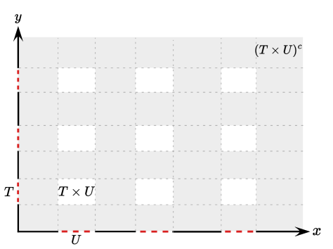
Figure 1: Truncation set in $\mathbb{R}^{2}$. The red dotted parts of the horizontal and vertical axes represent the unions of intervals $U$ and $T$, respectively. The white rectangles represent the set $T\times U$, and the remaining gray area of $\mathbb{R}^{2}$ is their complement, denoted as $(T\times U)^{c}$, on which we truncate the Gaussian distribution $\mathcal{N}((\varepsilon,0),\mathbf{I}_{2\times 2})$.

2 Preliminaries

Basic Notation We use the notation $[n]\stackrel{{\scriptstyle{\mathrm{\footnotesize def}}}}{{=}}\{1,\ldots,n\}$. We use $\mathbb{Z}$ for positive integers, and $\|\cdot\|_{2}$ for the $\ell_{2}$-norm of vectors. We use $\mathcal{N}(\bm{\mu},\mathbf{\Sigma})$ to denote the Gaussian with mean $\bm{\mu}$ and covariance matrix $\mathbf{\Sigma}$ and use $\phi_{\bm{\mu},\mathbf{\Sigma}}(\mathbf{x})$ for its probability density function. For other distributions, we will slightly abuse notation by using the same letter for a distribution and its pdf, e.g., we will denote by $P(\mathbf{x})$ the pdf of a distribution $P$.

Definition 2.1 (Truncated Gaussian).

For a set $S\subseteq\mathbb{R}^{d}$, a vector $\bm{\mu}\in\mathbb{R}^{d}$ and a PSD matrix $\mathbf{\Sigma}\in\mathbb{R}^{d\times d}$, we define $\mathcal{N}(\bm{\mu},\mathbf{\Sigma},S)$ to be the Gaussian with mean $\mathcal{N}(\bm{\mu},\mathbf{\Sigma})$ after truncation using the set $S$, i.e., the distribution with the following pdf (where $\phi_{\bm{\mu},\mathbf{\Sigma}}$ denotes the pdf of $\mathcal{N}(\bm{\mu},\mathbf{\Sigma})$): $\phi_{\bm{\mu},\mathbf{\Sigma},S}(x):=Z^{-1}\mathds{1}(x\in S)\phi_{\bm{\mu},\mathbf{\Sigma}}(\mathbf{x})$, where $Z:=\int_{\mathbb{R}^{d}}\mathds{1}(x\in S)\phi_{\bm{\mu},\mathbf{\Sigma}}(\mathbf{x})\mathrm{d}\mathbf{x}$.

We now define Gaussian Surface Area (GSA), which has served as a complexity measure of sets in learning theory and related fields; see, e.g., [KOS08, Kan11, Nee14].

Definition 2.2 (Gaussian Surface Area).

For a Borel set $A\subseteq\mathbb{R}^{d}$, its Gaussian surface area is defined by $\Gamma(A)\stackrel{{\scriptstyle{\mathrm{\footnotesize def}}}}{{=}}\liminf_{\delta\to 0}\frac{\mathcal{N}(A_{\delta}\setminus A)}{\delta},$ where $A_{\delta}=\{x:\mathrm{dist}(x,A)\leq\delta\}$.

Additional Background on the SQ Model The main fact that we use from the SQ literature [FGR⁺13, DKS17] concerns the family of distributions which are standard Gaussian along every direction, except from a low-dimensional subspace, where they are forced to be equal to some other (non-Gaussian) distribution $A$.

Definition 2.3 (Hidden Direction Distribution).

For an $m$-dimensional distribution $A$ and a matrix $\mathbf{V}\in\mathbb{R}^{m\times d}$, we define the distribution $P_{A,\mathbf{V}}$ with pdf $A(\mathbf{V}\mathbf{x})(2\pi)^{-\frac{(d-m)}{2}}e^{-\frac{1}{2}\|\mathbf{x}-\mathbf{V}^{\top}\mathbf{V}\mathbf{x}\|_{2}^{2}}$.

The main result from [DKS17] is that, if $A$ is similar to Gaussian, in the sense that its first moments agree with those of $\mathcal{N}(\mathbf{0},\mathbf{I})$, then the hypothesis testing problem between $\mathcal{N}(\mathbf{0},\mathbf{I})$ and a distribution of the above family is hard for any SQ algorithm. The following fact shows formally this hardness. See Appendix A for related preliminaries and the proof of the fact below; $\chi^{2}(A,B)$ below is defined as $\int_{\mathbb{R}^{d}}A^{2}(\mathbf{x})/B(\mathbf{x})\,\mathrm{d}\mathbf{x}-1$.

Fact 2.4.

Let $d,k\in\mathbb{Z}$ and $m<d^{1/10}$ and $k<d^{c}$ for some sufficiently small constant $c>0$. Let $A$ be a distribution over $\mathbb{R}^{m}$ such that its first $k$ moments match the corresponding moments of $\mathcal{N}(\mathbf{0},\mathbf{I}_{m})$. Define the family $\mathcal{D}$ of distributions containing $P_{A,\mathbf{U}}$ (cf. Definition 2.3) for all matrices $\mathbf{U}\in\mathbb{R}^{m\times d}$ such that $\mathbf{U}\mathbf{U}^{\top}=\mathbf{I}_{m}$. Then, any SQ algorithm that distinguishes between $\mathcal{N}(\mathbf{0},\mathbf{I}_{d})$ and $\mathcal{D}$ requires either $2^{d^{\Omega(1)}}$ many queries, or at least one query with tolerance $d^{-\Omega(k)}\sqrt{\chi^{2}(A,\mathcal{N}(\mathbf{0},\mathbf{I}_{m}))}$.

3 SQ Lower Bound For Truncated Gaussians

In this section we formalize the proof strategy for Theorem 1.2 which had been informally described in Section 1.2. We will show a stronger version of that theorem, stated below, which concerns hypothesis testing between the standard Gaussian and a truncated Gaussian.

Theorem 3.1 (SQ Lower Bound; Hypothesis Testing Hardness).

Let $d,k\in\mathbb{Z}_{+}$, $\varepsilon>d^{-c}$ for some sufficiently small constant $c>0$, and $k\leq c/\varepsilon^{0.15}$. Let $\mathcal{C}$ be the class of all sets $S\subseteq\mathbb{R}^{d}$ with the properties that: (i) $S$ is a union of at most $k^{2}$-many $d$-dimensional rectangles, and (ii) $S$ has $O(1)$ Gaussian surface area and $\Omega(1)$ mass under the target Gaussian. Consider the hypothesis testing problem defined below:

1. Null Hypothesis: $D=\mathcal{N}(\mathbf{0},\mathbf{I})$.

2. Alternative Hypothesis: $P\in\mathcal{D}$, where $\mathcal{D}$ is the family of truncated Gaussians $\mathcal{N}(\bm{\mu},\mathbf{I},S)$ for all $\|\bm{\mu}\|_{2}\geq\varepsilon$ and $S\in\mathcal{C}$.

Then, any SQ algorithm that solves the above problem, either performs $2^{d^{\Omega(1)}}$ many queries or performs at least one query with tolerance $d^{-\Omega(k)}$.

Note that Theorem 3.1 implies immediately Theorem 1.2 by a straightforward reduction: One can first find $\bm{\mu}$ approximating the true mean up to error $\varepsilon/2$ and then reject the null hypothesis if $\|\bm{\mu}\|>\varepsilon/2$.

The end goal towards showing Theorem 3.1 is to establish the existence of the following two-dimensional truncated Gaussian distribution $A$ that matches $k=\mathrm{poly}(1/\varepsilon)$ moments with the standard Gaussian (Proposition 3.2).

Proposition 3.2.

Let $c>0$ be a sufficiently small absolute constant, $\varepsilon\in(0,c)$, and $k=c/\varepsilon^{0.15}$. There exists a distribution $A$ on $\mathbb{R}^{2}$, for which the following are true:

1. $A$ matches its first $k$ moments with the 2-dimensional standard Gaussian.

2. $\chi^{2}(A,\mathcal{N}(\mathbf{0},\mathbf{I}_{2}))=O(1)$.

3. Every distribution of the form $P_{A,\mathbf{V}}$ (cf. Definition 2.3) can be written as a truncated Gaussian $\mathcal{N}(\bm{\mu},\mathbf{\Sigma},S)$ for $\bm{\mu}=(\varepsilon,0)$, $\mathbf{\Sigma}=\mathbf{I}_{2}$ (the $2\times 2$ identity matrix) and some $S\subseteq\mathbb{R}^{d}$ which has mass (with respect to the target Gaussian) at least $1/2$ and Gaussian surface area at most $1$.

Having Proposition 3.2 at hand, then Theorem 1.2 follows from Fact 2.4.

The proof of Proposition 3.2 requires two key results (Lemmata 3.3 and 3.4). In Proposition 3.2, $A$ is a 2-dimensional distribution that matches moments with the standard normal. In the following lemmata, we construct independently each dimension of that distribution. The marginal on the $y$-axis will be a standard normal, conditioned on a union of $k$ intervals, as shown in Lemma 3.3 below. As mentioned in the proof sketch of Section 1.2, we want these intervals to have small mass, thus we will eventually use $\delta=\sqrt{\varepsilon}$ below. We defer the proof to Section 4.

Lemma 3.3.

For any $\delta\in(0,1)$ and $k\in\mathbb{Z}_{+}$ there exists a set $U\subseteq\mathbb{R}$ such that: $U$ is a union of $k$ intervals with $\Pr_{y\sim\mathcal{N}(0,1)}[y\in U]=\delta$ and for all $t=1,\ldots,k$ it holds

$$\operatorname*{\mathbf{E}}_{y\sim\mathcal{N}(0,1)}[y^{t}\;|\;y\not\in U]=\operatorname*{\mathbf{E}}_{y\sim\mathcal{N}(0,1)}[y^{t}]\;.$$ (1)

Next we construct the marginal of $A$ for the $x$-axis. In this case, we start with a Gaussian distribution with mean $\varepsilon$, and we reweight it with a $k$-piecewise constant function taking values in $\{1-\delta,1\}$ so that it matches $k$ moments with the standard normal. The reason why we use values in $\{1-\delta,1\}$ is because we have removed $\delta$ mass in our construction for the $y$-axis. This will be clearer when we provide the calculation that $A$ matches moments with the 2-dimensional Gaussian. The proof can be found on Section 5.

Lemma 3.4.

Let $c>0$ be a sufficiently small absolute constant and $\varepsilon\in(0,c)$. Let $\delta,k$ be parameters so that $\delta=\sqrt{\varepsilon}$ and $k=c/\varepsilon^{0.15}$. There exists a set $T\subseteq\mathbb{R}$ such that: $T$ is a union of $k$ intervals, $\Pr_{x\sim\mathcal{N}(\varepsilon,1)}[x\in T]\leq\varepsilon^{0.3}$, and for all $t=0,\ldots,k$ it holds

$$\operatorname*{\mathbf{E}}_{x\sim\mathcal{N}(\varepsilon,1)}[x^{t}(1-\delta\mathds{1}\{x\in T\})]Z^{-1}=\operatorname*{\mathbf{E}}_{x\sim\mathcal{N}(0,1)}[x^{t}]\;,$$ (2)

where $Z=\operatorname*{\mathbf{E}}_{x\sim\mathcal{N}(\varepsilon,1)}[1-\delta\mathds{1}\{x\in T\}]$.

Using Lemmata 3.3 and 3.4, we can prove Proposition 3.2 by letting

$$A(x,y)=\frac{\phi(x-\varepsilon)\phi(y)\mathds{1}((x,y)\not\in T\times U)}{Z}\;.$$

In particular, it can be seen that $A$ matches $k$ moments with the $2$-dimensional normal by a direct computation that uses (1), (2). We provide the proof below.

Proof of Proposition 3.2.

Let $T,U,\delta,Z$ as in Lemmata 3.3 and 3.4, we let $A$ to be a distribution defined by the following probability density function:

$$A(x,y)=\frac{\phi(x-\varepsilon)\phi(y)\mathds{1}((x,y)\not\in T\times U)}{Z}\;.$$ (3)

We start with Item 1. First we note that $A$ is indeed a valid distribution, i.e., the normalizing factor is correct.

$$Z =\int\limits_{-\infty}^{+\infty}\int\limits_{-\infty}^{+\infty}D(x,y)\mathrm{d}y\,\mathrm{d}x=\int\limits_{-\infty}^{+\infty}\phi(x-\varepsilon)\left(\mathds{1}(x\in T)\int_{y\not\in U}\phi(y)\mathrm{d}y+\mathds{1}(x\not\in T)\int\limits_{-\infty}^{+\infty}\phi(y)\mathrm{d}y\right)\mathrm{d}x$$

$$=\int\limits_{-\infty}^{+\infty}\phi(x-\varepsilon)\left(\mathds{1}(x\in T)(1-\delta)+\mathds{1}(x\not\in T)\right)\mathrm{d}x$$ (by Lemma 3.3)

$$=\int\limits_{-\infty}^{+\infty}\phi(x-\varepsilon)(1-\delta\mathds{1}(x\in T))\mathrm{d}x\;,$$

where the calculation essentially used the geometry of our sets (see also Figure 1): For any fixed $x$, there are two cases. If $x\not\in T$, then no Gaussian mass is removed from the $y$-integral; otherwise, a $(1-\delta)$ mass is removed (as explained in Lemma 3.3).

We can similarly see that $A$ matches the first $k$ moments with the standard two dimensional Gaussian: Let $t$ and $s$ be non-negative integers with $t+s\leq k$. Then,

$$\frac{1}{Z} \int\limits_{-\infty}^{+\infty}\int\limits_{-\infty}^{+\infty}x^{t}y^{s}\phi(x-\varepsilon)\phi(y)\mathds{1}((x,y)\not\in T\times U)\mathrm{d}y\,\mathrm{d}x$$ (4)

$$=\frac{1}{Z}\int\limits_{-\infty}^{+\infty}x^{t}\phi(x-\varepsilon)\left(\mathds{1}(x\in T)\int\limits_{y\not\in U}y^{s}\phi(y)\mathrm{d}y+\mathds{1}(x\not\in T)\int\limits_{-\infty}^{+\infty}y^{s}\phi(y)\mathrm{d}y\right)\mathrm{d}x$$ (5)

$$=\frac{1}{Z}\int\limits_{-\infty}^{+\infty}x^{t}\phi(x-\varepsilon)\int\limits_{-\infty}^{+\infty}y^{s}\phi(y)\left(\mathds{1}(x\in T)(1-\delta)+\mathds{1}(x\not\in T)\right)\mathrm{d}y\mathrm{d}x$$ (by Lemma 3.3)

$$=\int\limits_{-\infty}^{+\infty}x^{t}\frac{\phi(x-\varepsilon)(1-\delta\mathds{1}(x\in T))}{Z}\mathrm{d}x\int\limits_{-\infty}^{+\infty}y^{s}\phi(y)\mathrm{d}y$$ (6)

$$=\int\limits_{-\infty}^{+\infty}x^{t}\phi(x)\mathrm{d}x\int\limits_{-\infty}^{+\infty}y^{s}\phi(y)\mathrm{d}y\;.$$ (by Lemma 3.4)

Finally, it is easy to see that the chi-square of $A$ is $O(1)$.

$$\chi^{2}(A,\mathcal{N}(\mathbf{0},\mathbf{I}_{2})) =\int\limits_{-\infty}^{+\infty}\int\limits_{-\infty}^{+\infty}\frac{A^{2}(x,y)}{\phi(x)\phi(y)}\mathrm{d}y\mathrm{d}x-1$$

$$=\int\limits_{-\infty}^{+\infty}\frac{\phi^{2}(x-\varepsilon)}{\phi(x)}\int\limits_{-\infty}^{+\infty}\phi(y)\mathds{1}((x,y)\not\in T\times U)\mathrm{d}y\mathrm{d}x-1$$

$$\leq\int\limits_{-\infty}^{+\infty}\frac{\phi^{2}(x-\varepsilon)}{\phi(x)}\mathrm{d}x=\chi^{2}(\mathcal{N}(\varepsilon,1),\mathcal{N}(0,1))=e^{\varepsilon^{2}}\;.$$

We move to Item 3. The fact that $P_{A,\mathbf{V}}$ is a truncated Gaussian follows trivially by our definitions. The Gaussian surface area bound comes from the fact that $T\times U$ is a union of at most $k^{2}$ many rectangles, each with perimeter $O(\delta)$ (this is because the sets $T$ and $U$ from Lemmata 3.3 and 3.4 have mass at most $O(\delta)$). Using $\delta=\sqrt{\varepsilon}$ and $k\ll 1/\varepsilon^{1/4}$, we obtain that the Gaussian surface area is at most $1$. ∎

4 Proof of Lemma 3.3

Regarding Lemma 3.3, we need to find a union $U$ of $k$ intervals such that the truncated version of $\mathcal{N}(0,1)$ on these intervals matches moments with $\mathcal{N}(0,1)$, and the mass of $U$ under $\mathcal{N}(0,1)$ is equal to a parameter $\delta$ of our choice. The proof strategy is the following: First, we note in Claim 4.1 that it suffices to find a piecewise constant function $f:\mathbb{R}\to\{-\delta,1-\delta\}$ such that $\operatorname*{\mathbf{E}}_{z\sim\mathcal{N}(0,1)}[z^{t}f(z)]=0$, i.e., the weighted by $f$ moments of $\mathcal{N}(0,1)$ are zero. Claim 4.1 implies that once such a function $f$ is found, Lemma 3.3 follows by letting the set $U$ be the union of all the intervals where $f(z)>0$. We proceed to showing the existence of $f$ through a two-step process. We start with an explicit construction in Claim 4.2. Although capable of making the weighted moments arbitrarly close to zero, this construction yields a function with a significantly larger number of pieces than $k$. We are then able to reduce the number of pieces down to the desired count of $k$ using a technique from [DKZ20], implemented in Proposition 4.3.

Claim 4.1.

Let $U\subseteq\mathbb{R}$ and $t\in\mathbb{Z}_{+}$ be a set and an integer. Define the piecewise constant function

$$f(z)=\begin{cases}1-\delta,&z\in U\\ -\delta,&z\not\in U\;,\end{cases}$$

with $\delta:=\Pr_{z\sim\mathcal{N}(0,1)}[z\in U]$. The following three statements are equivalent:

1. $\operatorname*{\mathbf{E}}_{z\sim\mathcal{N}(0,1)}[z^{t}f(z)]=0$.

2. $\operatorname*{\mathbf{E}}_{z\sim\mathcal{N}(0,1)}[z^{t}|z\in U]=\operatorname*{\mathbf{E}}_{z\sim\mathcal{N}(0,1)}[z^{t}]$.

3. $\operatorname*{\mathbf{E}}_{z\sim\mathcal{N}(0,1)}[z^{t}|z\not\in U]=\operatorname*{\mathbf{E}}_{z\sim\mathcal{N}(0,1)}[z^{t}]$.

Proof.

We first show the equivalence between Item 2 and Item 3. We assume Item 2 and show Item 3 (the other direction is identical):

$$\operatorname*{\mathbf{E}}_{z\sim\mathcal{N}(0,1)}[z^{t}] =\operatorname*{\mathbf{E}}_{z\sim\mathcal{N}(0,1)}[z^{t}\mathds{1}(z\in U)]+\operatorname*{\mathbf{E}}_{z\sim\mathcal{N}(0,1)}[z^{t}\mathds{1}(z\not\in U)]$$

$$=\delta\operatorname*{\mathbf{E}}_{z\sim\mathcal{N}(0,1)}[z^{t}|z\in U]+(1-\delta)\operatorname*{\mathbf{E}}_{z\sim\mathcal{N}(0,1)}[z^{t}|z\not\in U]$$ (7)

$$=\delta\operatorname*{\mathbf{E}}_{z\sim\mathcal{N}(0,1)}[z^{t}]+(1-\delta)\operatorname*{\mathbf{E}}_{z\sim\mathcal{N}(0,1)}[z^{t}|z\not\in U]\;,$$

where the last line used Item 2. Rearranging, this means that $\operatorname*{\mathbf{E}}_{z\sim\mathcal{N}(0,1)}[z^{t}|z\not\in U]=\operatorname*{\mathbf{E}}_{z\sim\mathcal{N}(0,1)}[z^{t}]$.

We now prove that Item 2 and Item 3 imply Item 1, i.e., $\operatorname*{\mathbf{E}}_{z\sim\mathcal{N}(0,1)}[z^{t}f(z)]=0$.

$$\frac{1}{\delta(1-\delta)}\operatorname*{\mathbf{E}}_{z\sim\mathcal{N}(0,1)}[z^{t}f(z)] =\frac{1}{\delta}\operatorname*{\mathbf{E}}_{z\sim\mathcal{N}(0,1)}[z^{t}\mathds{1}(z\in U)]-\frac{1}{1-\delta}\operatorname*{\mathbf{E}}_{z\sim\mathcal{N}(0,1)}[z^{t}\mathds{1}(z\not\in U)]$$

$$=\operatorname*{\mathbf{E}}_{z\sim\mathcal{N}(0,1)}[z^{t}|z\in U]-\operatorname*{\mathbf{E}}_{z\sim\mathcal{N}(0,1)}[z^{t}|z\not\in U]=0\;,$$ (8)

where the last equality is due to the part we showed earlier.

The direction from Item 1 to Item 2 is similar: By writing out $\operatorname*{\mathbf{E}}_{z\sim\mathcal{N}(0,1)}[z^{t}f(z)]=0$ similarly to (8) we can see that $\operatorname*{\mathbf{E}}_{z\sim\mathcal{N}(0,1)}[z^{t}|z\in U]=\operatorname*{\mathbf{E}}_{z\sim\mathcal{N}(0,1)}[z^{t}|z\not\in U]$. Then, using this in (7) we get that both conditional expectations are equal to $\operatorname*{\mathbf{E}}_{z\sim\mathcal{N}(0,1)}[z^{t}]$. ∎

Next we explicitly construct a piecewise constant function from $\mathbb{R}$ to $\{-\delta,1-\delta\}$ that achieves zero weighted moments (or, more accurately, arbitrarily small weighted moments).

Claim 4.2.

For any $\eta>0$ and $\delta\in(0,1)$, there exists a $(k\log(1/\eta))^{2k}/\eta$-piecewise constant function $g_{\eta}:\mathbb{R}\to\{1-\delta,-\delta\}$ such that $|\operatorname*{\mathbf{E}}_{z\sim\mathcal{N}(0,1)}[g_{\eta}(z)z^{t}]|\leq\eta$, for all $t=0,1,\ldots,k$ and $\Pr_{z\sim\mathcal{N}(0,1)}[f(z)=1-\delta]\in[\delta-\eta,\delta+\eta]$.

We sketch the proof of Claim 4.2, with the full version being deferred to Section 4.1. The idea is that we partition the real line into intervals $A_{i}=[is,(i+1)s]$ for $i\in\mathbb{Z}$ using a small step size $s$. For each $i\in\mathbb{Z}$, we further split $A_{i}$ into two parts $A_{i}^{+}:=[is,(i+\delta)s]$ and $A_{i}^{-}:=[(i+\delta)s,(i+1)s]$, i.e., the ratio of the sub-intervals’ length is $\delta/(1-\delta)$. We define $g_{\eta}(z)=1-\delta$ on $A_{i}^{+}$ and $g_{\eta}(z)=-\delta$ on $A_{i}^{-}$ for all $i$. The main argument is that since the Gaussian density does not change by much inside $A_{i}$, the contribution to the moment integral from the sub-intervals $A_{i}^{+}$ and $A_{i}^{-}$ must approximately adhere to the ratio of the sub-intervals’ lengths, i.e.,

$$\frac{\int_{A_{i}^{+}}z^{t}\phi(z)\mathrm{d}z}{\int_{A_{i}^{-}}z^{t}\phi(z)\mathrm{d}z}=\frac{\delta}{1-\delta}(1+\xi_{i})$$ (9)

for some small $\xi_{i}$. In fact, we can show it for $|\xi_{i}|=O(is^{2})$ using a polynomial approximation for the density function $\phi(z)$. The important part is that we can control $|\xi_{i}|$ using the step size $s$. Finally,

$$\left|\operatorname*{\mathbf{E}}_{z\sim\mathcal{N}(0,1)}[g_{\eta}(z)z^{t}]\right| =\left|\sum_{i\in\mathbb{Z}}\int_{z\in A_{i}}g_{\eta}(z)z^{t}\phi(z)\mathrm{d}z\right|\leq\sum_{i\in\mathbb{Z}}\left|(1-\delta)\int_{z\in A_{i}^{+}}z^{t}\phi(z)\mathrm{d}z-\delta\int_{z\in A_{i}^{-}}z^{t}\phi(z)\mathrm{d}z\right|$$

$$\leq\sum_{i\in\mathbb{Z}}\left|\xi_{i}\,\delta\int_{z\in A_{i}^{-}}f(z)z^{t}\phi(z)\mathrm{d}z\right|<\eta\;.$$ (using (9))

The last step above amounts to a sufficiently small $s$ so that $\xi_{i}$ becomes sufficiently small and makes the entire right hand side less than $\eta$. There are additional details needed to formalize this, such as noting that the summation does not need to cover the entire range of $i\in\mathbb{Z}$. We defer these details to Section 4.1.

The final step is to reduce the number of pieces from $(k\log(1/\eta))^{2k}/\eta$ down to $k$. To this end, we use the proposition below which shows that we can start with a $t>k$ piecewise constant function and decrease the number of pieces to $k$ without changing the desired properties of the function. An analogous statement was shown in [DKZ20]; here we require a generalization of this for all continuous distributions and any sequence of moments. The main idea of the proof is to model the endpoints of the intervals as a differential equation. To do so, we start with an instance that has many more endpoints than our goal, i.e., the instance has $t$ endpoints, and the first $k$ moments of this distribution have specific values. One can model this as a vector-valued function $\mathbf{M}(z_{1},\ldots,z_{t}):\mathbb{R}^{t}\mapsto\mathbb{R}^{k}$, where $z_{1},\ldots,z_{t}$ are the endpoints and $\mathbf{M}_{i}$ is the value of the $i$-th moment. Our task is to move the endpoints $z_{i}$ until two of them coincide or one of them goes to infinity, while keeping the vector $\mathbf{M}$ constant (so that the moments will continue to satisfy our assumptions). This is achieved by finding a specific $\mathbf{u}(z):\mathbb{R}\mapsto\mathbb{R}^{t}$ with the properties that $\mathbf{u}(0)=[z_{1},\ldots,z_{t}]$ (so that the initial conditions satisfy our moment assumptions), $\mathrm{d}\mathbf{M}(\mathbf{u}_{1}(z),\ldots,\mathbf{u}_{t}(z))/\mathrm{d}z=\mathbf{0}$ (so that the moments remain constant), and $\mathrm{d}\mathbf{u}_{t}(z)/\mathrm{d}z=1$ (so that at least one endpoint will be removed, i.e., in the worst case the $t$-th endpoint goes to infinity). One can show that such a function $\mathbf{u}$ always exists, as long as $t>k+1$. For completeness, we provide a proof in Appendix B.1.

Proposition 4.3.

Let $k,\ell$ be positive integers with $\ell\geq k+1$ and $a,b\in\mathbb{R}$ with $b>a$. Let $D$ be a continuous distribution over $\mathbb{R}$ and let $\nu_{0},\ldots,\nu_{k-1}\in\mathbb{R}$. If for any $\eta>0$ there exists an at most $\ell$-piecewise constant function $g_{\eta}:\mathbb{R}\to\{a,b\}$ such that $|\operatorname*{\mathbf{E}}_{z\sim D}[g_{\eta}(z)z^{t}]-\nu_{t}|\leq\eta$ for every non-negative integer $t<k$, then there exists an at most $(k+1)$-piecewise constant function $f:\mathbb{R}\to\{a,b\}$ such that $\operatorname*{\mathbf{E}}_{z\sim D}[f(z)z^{t}]=\nu_{t}$, for every non-negative integer $t<k$.

Having the above at hand, the proof of Lemma 3.3 follows from Claim 4.2 and Proposition 4.3 applied with $a=-\delta$, $b=1+\delta$, $D=\mathcal{N}(0,1)$. The set $U$ that satisfies the conclusion of Lemma 3.3 is the set of intervals on which $f(z)>0$.

4.1 Proof of Claim 4.2

Let $C$ be a sufficiently large absolute constant. Fix the parameters $s:=0.01\eta/(k\log(1/\eta))^{k}$, $i_{\max}=10\log^{k}(1/\eta)/s$ throughout the proof. We also define $U^{+}$ and $U^{-}$ to be the unions of intervals in the positive and negative part of the real line as shown below. We define them so that their union $U=U^{+}\cup U^{-}$ is symmetric around zero:

$$U^{+} :=\left(\bigcup_{i=0}^{i_{\max}-1}[is,(i+\delta)s]\right)\cup[i_{\max}s,+\infty)\;,$$

$$U^{-} :=\left(\bigcup_{i=0}^{i_{\max}-1}[-(i+\delta)s,-is]\right)\cup[-\infty,-i_{\max}s)\;.$$

Finally define the piecewise constant function

$$g_{\eta}(z):=\begin{cases}1-\delta&,z\in U\\ -\delta&,z\not\in U\;.\end{cases}$$

First, we note that because of symmetry of $g_{\eta}(z)$ around zero

$$\left|\operatorname*{\mathbf{E}}_{z\sim\mathcal{N}(0,1)}[g_{\eta}(z)z^{t}]\right|\leq\left|\int_{-\infty}^{0}g_{\eta}(z)z^{t}\phi(z)\mathrm{d}z\right|+\left|\int_{0}^{+\infty}g_{\eta}(z)z^{t}\phi(z)\mathrm{d}z\right|=2\left|\int_{0}^{+\infty}g_{\eta}(z)z^{t}\phi(z)\mathrm{d}z\right|\;.$$ (10)

Therefore, in everything that follows, it suffices to only consider the integral on the positive part of the real line.

Our goal is to bound (10) by $\eta$. As a first step, we need the following bound on the ratio of consecutive pieces of the moment integral:

$$\frac{\int_{is}^{(i+\delta)s}z^{t}\phi(z)\mathrm{d}z}{\int_{(i+\delta)s}^{(i+1)s}z^{t}\phi(z)\mathrm{d}z}\leq\frac{\delta s((i+\delta)s)^{t}\phi(is)}{(1-\delta)s((i+\delta)s)^{t}\phi((i+1)s)}\leq\frac{\delta}{1-\delta}e^{is^{2}+s^{2}/2}\leq\frac{\delta}{1-\delta}(1+2is^{2})\;,$$ (11)

where we used the minimum and maximum values that the $z^{t}\phi(z)$ takes in each integral, and then used that $1+x\leq e^{x}\leq 1+1.1x$ for all $x<0.1$, where we applied this with $x=is^{2}\leq i_{\max}s^{2}$ which is indeed less than $0.1$ for our choice of $s,i_{\max}$.

We can now proceed to bound (10). We start with the upper bound; see below for step by step explanations:

$$\int_{0}^{+\infty} g_{\eta}(z)z^{t}\phi(z)\mathrm{d}z$$

$$=\int_{i_{\max}s}^{+\infty}z^{t}\phi(z)\mathrm{d}z+\sum_{i=0}^{i_{\max}-1}\int_{is}^{(i+1)s}g_{\eta}(z)z^{t}\phi(z)\mathrm{d}z$$

$$\leq\frac{\eta}{4}+\sum_{i=0}^{i_{\max}-1}\left\{(1-\delta)\int_{is}^{(i+\delta)s}z^{t}\phi(z)\mathrm{d}z-\delta\int_{(i+\delta)s}^{(i+1)s}z^{t}\phi(z)\mathrm{d}z\right\}$$ (12)

$$=\frac{\eta}{4}+\sum_{i=0}^{i_{\max}-1}\left\{(1-\delta)\frac{\delta}{1-\delta}(1+2is^{2})\int_{(i+\delta)s}^{(i+1)s}z^{t}\phi(z)\mathrm{d}z-\delta\int_{(i+\delta)s}^{(i+1)s}z^{t}\phi(z)\mathrm{d}z\right\}$$ (13)

$$=\frac{\eta}{4}+\sum_{i=0}^{i_{\max}-1}\left\{2i\delta s^{2}\int_{(i+\delta)s}^{(i+1)s}z^{t}\phi(z)\mathrm{d}z\right\}$$

$$\leq\frac{\eta}{4}+20s\log^{k}(1/\eta)\sum_{i=0}^{i_{\max}-1}\int_{(i+\delta)s}^{(i+1)s}z^{t}\phi(z)\mathrm{d}z$$ (14)

$$\leq\frac{\eta}{4}+20\delta s\log^{k}(1/\eta)\int_{0}^{+\infty}z^{t}\phi(z)\mathrm{d}z$$ (15)

$$\leq\frac{\eta}{4}+20s\log^{k}(1/\eta)(t-1)!!$$ (16)

$$\leq\frac{\eta}{4}+\frac{\eta}{4}=\frac{\eta}{2}\;.$$ (17)

We now justify each step in the above derivations. (12) uses the Gaussian concentration inequality $\Pr[z^{t}>\beta]\leq e^{-\beta^{2/t}/2}$ for $\beta=i_{\max}s=10\log^{k}(1/\eta)$. (13) holds because of (11). (14) follows because $is\leq 10\log^{k}(1/\eta)$. (16) uses the Gaussian moment bound. (17) holds because $(t-1)!!\leq t^{t}\leq k^{k}$ and the choice $s:=0.01\eta/(k^{k}\log^{k}(1/\eta))$.

The other direction, i.e., $\int_{0}^{+\infty}g_{\eta}(z)z^{t}\phi(z)\mathrm{d}z\geq-\eta/2$, can be shown with a similar argument:

$$\int_{0}^{+\infty}g_{\eta}(z)z^{t}\phi(z)\mathrm{d}z \geq\sum_{i=0}^{i_{\max}-1}\left\{-\delta\int_{(i+\delta)s}^{(i+1)s}z^{t}\phi(z)\mathrm{d}z+(1-\delta)\int_{(i+1)s}^{(i+1+\delta)s}z^{t}\phi(z)\mathrm{d}z\right\}$$

$$\geq\sum_{i=0}^{i_{\max}-1}\left\{-\delta\left(\frac{1-\delta}{\delta}\right)(1+2is^{2})+1-\delta\right\}\int_{(i+1)s}^{(i+1+\delta)s}z^{t}\phi(z)\mathrm{d}z$$

$$\geq-\sum_{i=0}^{i_{\max}-1}2(1-\delta)is^{2}\int_{(i+1)s}^{(i+1+\delta)s}z^{t}\phi(z)\mathrm{d}z\geq-20s\log^{k}(1/\eta)(t-1)!!\geq-\frac{\eta}{4}\;,$$

where instead of (11) we used the bound $\int_{(i+\delta)s}^{(i+1)s}z^{t}\phi(z)\mathrm{d}z\leq\frac{1-\delta}{\delta}(1+2is^{2})\int_{(i+1)s}^{(i+1+\delta)s}z^{t}\phi(z)\mathrm{d}z$, which can be shown in a similar manner.

We finally calculate the $\Pr[z\in U]$ (which is the same as $\Pr[g_{\eta}(z)=1-\delta]$), as follows

$$\Pr[z\in U] \leq 2\sum_{i=0}^{i_{\max}-1}\int_{is}^{(i+\delta)s}\phi(z)\mathrm{d}z=2\sum_{i=0}^{i_{\max}-1}\delta(1+2is^{2})\int_{(i+1)s}^{(i+2)s}\phi(z)\mathrm{d}z$$

$$=2\delta\sum_{i=0}^{i_{\max}-1}\int_{(i+1)s}^{(i+2)s}\phi(z)\mathrm{d}z+4\delta\sum_{i=0}^{i_{\max}-1}is^{2}\int_{(i+1)s}^{(i+2)s}\phi(z)\mathrm{d}z$$

$$\leq 2\delta\sum_{i=0}^{i_{\max}-1}\int_{(i+1)s}^{(i+2)s}\phi(z)\mathrm{d}z+40s\log^{k}(1/\eta)\sum_{i=0}^{i_{\max}-1}\int_{(i+1)s}^{(i+2)s}\phi(z)\mathrm{d}z$$

$$\leq 2\delta\frac{1}{2}+20s\log^{k}(1/\eta)\frac{1}{2}\leq\delta+\eta\;,$$

where the first line uses a ratio bound similar to (11), the third line uses that $is\leq 10\log^{k}(1/\eta)$, and the last line uses that $\sum_{i}\int_{(i+1)s}^{(i+2)s}\phi(z)\mathrm{d}z\leq 1/2$ and that $s:=0.01\eta/(k^{k}\log^{k}(1/\eta))$.

Similarly, it can be shown that $\Pr[z\in U]\geq\delta-\eta$, which completes the proof. ∎

5 Proof of Lemma 3.4

The high-level approach for proving Lemma 3.4 is to first show a relaxed version of the statement, where the “hard set $T$” is replaced by a “soft set $f$” which is a function $f:\mathbb{R}\to[0,1]$. That is, define the distribution

$$P_{f}(x)=\phi(x-\varepsilon)(1-\delta f(x))Z^{-1}\;\;\text{for}\;\;Z:=\int_{-\infty}^{+\infty}\phi(x-\varepsilon)(1-\delta f(x))\mathrm{d}x\;.$$ (18)

We seek to find an $f:\mathbb{R}\to[0,1]$ satisfying the following two constraints:

1. (Moment matching) $\operatorname*{\mathbf{E}}_{x\sim P_{f}}[x^{t}]=\operatorname*{\mathbf{E}}_{x\sim\mathcal{N}(0,1)}[x^{t}]$, and

2. ($f$ has small mass) $Z=1-\delta\varepsilon^{0.3}$

Note that this is indeed a relaxed version of the statement of Lemma 3.4 which results by replacing the $\mathds{1}(x\in T)$ by $f(x)$: the first constraint above is the relaxed version of (1) and the second constraint is equivalent to $\operatorname*{\mathbf{E}}_{x\sim\mathcal{N}(\varepsilon,1)}[f(x)]\leq\varepsilon^{0.3}$, which is the relaxed version of the constraint $\Pr_{x\sim\mathcal{N}(\varepsilon,1)}[x\in T]\leq\varepsilon^{0.3}$ appearing in Lemma 3.4. Once we find such an $f$, we can convert it to a “hard set” $T$ which is a union of intervals by using a randomized rounding technique, similar to [DKZ20]. Finally, that technique does not ensure any guarantees on the number of intervals produced, but using Proposition 4.3 as in the previous section, we can bring this number down to $k$.

We will prove Item 1 and Item 2 that were listed before in two steps: We will find an $f$ consisting of two parts $f(x)=f_{1}(x)+f_{2}(x)$ with $f_{1}(x)\in[\varepsilon,1/2]$ and $f_{2}(x)\in[-\varepsilon,\varepsilon]$ (so that overall $f(x)\in[0,1])$. For the first part (cf. Claim 5.1), the idea is to start by $f_{1}$ being the function that would make the distribution $P_{f_{1}}$ (cf. notation of (18)) exactly the same as $\phi(x)$ (the pdf of $\mathcal{N}(0,1)$), and then clip $f_{1}(x)$ so that it only takes values in $[\varepsilon,1/2]$. The important observation is that the clipping only happens for $x$ with large $|x|$. Thus, already $P_{f_{1}}$ is equal to $\phi(x)$ on big part of the real line. The remaining part contributes negligible amount to the moments, thus we can correct the moments by adding a correction term $f_{2}(x)$ to $f_{1}(x)$. We find $f_{2}$ by finding an appropriate polynomial using a technique from [DKS17].

We now implement the two steps of the proof. For the first one, (regarding $f_{1}$), we have the following.

Claim 5.1.

Fix $\delta=\sqrt{\varepsilon}$. There exists an $f_{1}:\mathbb{R}\to[\varepsilon,1/2]$ such that $\int_{-\infty}^{+\infty}\phi(x-\varepsilon)(1-\delta f_{1}(x))\mathrm{d}x=1-\delta\varepsilon^{0.3}$ and the distribution with pdf

$$P_{f_{1}}(x)=\frac{\phi(x-\varepsilon)(1-\delta f_{1}(x))}{1-\delta\varepsilon^{0.3}}$$

satisfies $q(x)=\phi(x)$ for all $x$ with $|x|\leq 1/\varepsilon^{2/11}$.

Proof.

Define $\xi:=\delta\varepsilon^{0.3}=\varepsilon^{0.8}$ (recalling that $\delta=\sqrt{\varepsilon})$. For notational convenience, we will consider the following equivalent statement of our claim: there exists an $h:\mathbb{R}\to[1-\delta\varepsilon,1-\delta/2]$ such that $\int_{-\infty}^{+\infty}\phi(x-\varepsilon)h(x)\mathrm{d}x=1-\xi=1-\delta\varepsilon^{0.3}$ and $\frac{\phi(x-\varepsilon)h(x)}{1-\xi}=\phi(x)$ for all $x$ with $|x|\leq 1/\varepsilon^{2/11}$; the original statement would follow by this after letting $f_{1}(x)=(1-h(x))/\delta$).

To show our claim, let us first consider the function $\tilde{h}$, which we define so that

$$\frac{\phi(x-\varepsilon)\tilde{h}(x)}{1-\xi}=\phi(x)\quad\text{for all $x\in\mathbb{R}$}\;.$$

That is, we define $\tilde{h}(x):=\exp(\varepsilon^{2}/2-\varepsilon x)(1-\xi)$. Then, we define $h$ to the version of $\tilde{h}$ which is clipped in the interval $[1-\delta\varepsilon,1-\delta/2]$, i.e.,

$$h(x):=\begin{cases}1-\delta\varepsilon,&\text{if $\tilde{h}(x)>1-\delta\varepsilon$}\\ \tilde{h}(x)&\text{if $1-\delta/2\leq\tilde{h}(x)\leq 1-\delta\varepsilon$}\\ 1-\delta/2,&\text{if $\tilde{h}(x)<1-\delta/2$}\;.\end{cases}$$

Finally, it remains to verify that the clipping happens only for $x$ with $|x|>1/\varepsilon^{2/11}$. First, note that $\tilde{h}$ is a decreasing function. By plugging $x=-1/\varepsilon^{2/11}$ we can see that $h(-1/\varepsilon^{2/11})=1-\Theta(\varepsilon^{4/5})$ (we can see that by using a polynomial approximation for the $e^{x}$ function), which is less than the clipping threshold of $1-\delta\varepsilon=1-\varepsilon^{1.5}$. Thus, by monotonicity of $h$, $\sup\{x\in\mathbb{R}:h(x)>1-\delta\varepsilon\}<-1/\varepsilon^{2/11}$. Similarly, we can check the other boundary. ∎

We now move to the second part of the argument, which aims to find an $f_{2}:\mathbb{R}\to[-\varepsilon,\varepsilon]$ such that when $f=f_{1}+f_{2}$, the moments of $P_{f}$ get corrected and equal to those of $\mathcal{N}(0,1)$. Fix $C=\sqrt{\varepsilon}$ and $\xi=\delta\varepsilon^{0.3}=1-\varepsilon^{0.8}$. We will search for an $f_{2}$ of the particular form below

$$f_{2}(x)=\frac{1-\xi}{\delta}\frac{p(x)}{\phi(x-\varepsilon)}\mathds{1}(|x|\leq C)\;,$$ (19)

for some appropriate polynomial with $\int_{-C}^{C}p(x)\mathrm{d}x=0$ and small $|p(x)|$ for all $x\in[-C,C]$. We now show how to find that polynomial and ensure the above properties. Our moment-matching constraint is the following (note that the normalization of the distribution is still $1-\xi$, because of the property $\int_{-C}^{C}p(x)\mathrm{d}x=0$):

$$\int_{-\infty}^{+\infty}x^{t}\frac{\phi(x-\varepsilon)(1-\delta f_{1}(x)-\delta f_{2}(x))}{1-\xi}\mathrm{d}x=\int_{-\infty}^{+\infty}x^{t}\phi(x)\mathrm{d}x\;.$$

By letting $P_{f_{1}}(x)=\frac{\phi(x-\varepsilon)(1-\delta f_{1}(x))}{1-\xi}$ as in Claim 5.1, the above is equivalent to

$$\int_{-C}^{+C}x^{t}p(x)\mathrm{d}x=\int_{-\infty}^{+\infty}x^{t}P_{f_{1}}(x)\mathrm{d}x-\int_{-\infty}^{+\infty}x^{t}\phi(x)\mathrm{d}x\;.$$ (20)

The rest of the proof mirrors that in [DKS17]. By Claim 5.8 in [DKS17], there exists a unique polynomial $p$ satisfying (20), which has the form $p(x)=\sum_{i=0}^{k}a_{i}P_{i}(x/C)$, where $P_{i}$ is the $i$-th Legendre polynomial and $a_{i}=\frac{2i+1}{2C}\int_{-C}^{C}P_{i}(x/C)p(x)\mathrm{d}x$. We want to show that $|a_{i}|=O(i\varepsilon^{5})$. First we note why this would be enough. This is because, by properties of the Legendre polynomials (see Appendix A for basic properties that we will use), it would imply that $|p(x)|=O(\sum_{i=1}^{k}|a_{i}|)=O(k^{2}\varepsilon^{5})$ for all $x\in[-C,C]$. We would then be done, because after combining with (19), we would obtain that for all $x\in[-C,C]$ it holds

$$|f_{2}(x)|\leq\frac{(1-\xi)|p(x)|}{\delta\phi(x-\varepsilon)}\leq\frac{O(\varepsilon^{5}k^{2})}{\delta\phi(x-\varepsilon)}<\varepsilon\;,$$

where we used $\delta=\sqrt{\varepsilon}$, $k\leq c/\varepsilon^{0.15}$, and that $\phi(x-\varepsilon)\geq 1/3$ for all $x\in[-1,1]$. We conclude by showing that $|a_{i}|=O(i\varepsilon^{5})$. First, by orthogonality of the $P_{i}$’s and (20),

$$\left|\int_{-C}^{C}P_{i}(x/C)p(x)\mathrm{d}x\right| =\left|\int_{-\infty}^{+\infty}P_{i}(x/C)(\phi(x)-P_{f_{1}}(x))\mathrm{d}x\right|=\left|\int_{|x|>1/\varepsilon^{2/11}}P_{i}(x/C)(\phi(x)-P_{f_{1}}(x))\mathrm{d}x\right|$$

$$\leq\left|\int_{|x|>1/\varepsilon^{2/11}}P_{i}(x/C)\phi(x)\mathrm{d}x\right|+\left|\int_{|x|>1/\varepsilon^{2/11}}P_{i}(x/C)P_{f_{1}}(x)\mathrm{d}x\right|\;,$$

where the second step used that $P_{f_{1}}(x)=\phi(x)$ for all $x$ with $|x|\leq 1/\varepsilon^{2/11}$ by Claim 5.1. We will show the bound for the first term (the other one is similar).

Claim 5.2.

Fix $C=\sqrt{\varepsilon}$, and let $P_{i}$ denote the $i$-Legendre polynomial and $p$ be the solution to (20). Then, $\left|\int_{|x|>1/\varepsilon^{2/11}}P_{i}(x/C)\phi(x)\mathrm{d}x\right|=O(\varepsilon^{5})$.

Proof.

We will use the known property that the $j$-th Legendre polynomial can be written as $P_{j}(x)=\frac{1}{2^{i}}\sum_{j=0}^{\lfloor i/2\rfloor}\binom{i}{j}\binom{2i-2j}{i}x^{i-2j}$. We will also use that there is negligible mass at the tails $|x|>1/\varepsilon^{2/11}$. We have that

$$\left|\int_{-C}^{C}P_{i}(x/C)p(x)\mathrm{d}x\right| =O((k/C)^{3k})\int_{|x|>1/\varepsilon^{2/11}}|x|^{k}\phi(x)\mathrm{d}x$$

$$\leq O((k/C)^{3k})\int_{|x|>1/\varepsilon^{2/11}}|x|^{k}e^{-x^{2}/2}\mathrm{d}x$$

$$\leq O((k/C)^{3k})\varepsilon^{10k}=O((k/\sqrt{\varepsilon})^{3k})\varepsilon^{10k}=O(\varepsilon^{5})\;,$$

where the first step bounds the binomial coefficients by $k^{k}$ and in the last line uses that for any $|x|>100k\log(1/\varepsilon)=\varepsilon^{-3/20}\log(1/\varepsilon)$ (recall that $k=\Theta(\varepsilon^{3/20})$) it holds $|x|^{k}e^{-x^{2}/2}<\varepsilon^{10k}/x^{2}$, in order to bound $\int_{|x|>\varepsilon^{-2/11}}|x|^{k}e^{-x^{2}/2}\mathrm{d}x\leq\int_{|x|>1}|x|^{k}e^{-x^{2}/2}\mathrm{d}x\leq\varepsilon^{10k}\int_{|x|>1}x^{-2}\mathrm{d}x\leq\varepsilon^{10k}$.

∎

This completes the proof of Items 1 and 2. We next use a randomized rounding technique similar to [DKZ20], in order to convert this continuous $f$ to a piecewise constant $\tilde{f}:\mathbb{R}\to\{0,1\}$, i.e., a hard set. We show the following in Section 5.1:

Claim 5.3.

For any $\eta>0$ there exists a $((k\log(1/\eta))^{\mathrm{poly}(k)}/\eta^{2})$-piecewise constant function $\tilde{f}:\mathbb{R}\to\{0,1\}$ such that $\Pr_{x\sim\mathcal{N}(\varepsilon,1)}[\tilde{f}(x)]\leq 2\delta$ and for all $t=0,\ldots,k$ it holds $|\operatorname*{\mathbf{E}}_{x\sim\mathcal{N}(\varepsilon,1)}[x^{t}(1-\delta\tilde{f}(x))]Z^{-1}-\operatorname*{\mathbf{E}}_{x\sim\mathcal{N}(0,1)}[x^{t}]|\leq\eta$, where $Z=\operatorname*{\mathbf{E}}_{x\sim\mathcal{N}(\varepsilon,1)}[1-\delta\tilde{f}(x)]$.

The idea for Claim 5.3 is to split $\mathbb{R}$ into $[is,(i+1)s]$, for $i\in\mathbb{Z}$ and a sufficiently small size $s$, and to let $\tilde{f}(x)$ be constant in the interval $x\in[is,(i+1)s)$, taking the following values:

$$\tilde{f}(x)=\begin{cases}1,&\text{with probability $p_{i}:=\int_{is}^{(i+1)s}\phi(x-\varepsilon)f(x)\mathrm{d}x/\int_{is}^{(i+1)s}\phi(x-\varepsilon)\mathrm{d}x$}\\ 0,&\text{with probability $1-p_{i}$}\end{cases}$$ (21)

We want to show that $\operatorname*{\mathbf{E}}_{x\sim\mathcal{N}(\varepsilon,1)}[x^{t}(1-\delta\tilde{f}(x))]\approx\operatorname*{\mathbf{E}}_{x\sim\mathcal{N}(\varepsilon,1)}[x^{t}(1-\delta f(x))]$ (which we have already shown that is equal to $\operatorname*{\mathbf{E}}_{x\sim\mathcal{N}(0,1)}[x^{t}]$). Let $I_{i}:=\int_{is}^{(i+1)s}x^{t}\phi(x-\varepsilon)\delta(f(x)-\tilde{f}(x))\mathrm{d}x$ be the contribution due to the $i$-th interval. Then, using the Taylor approximation $x^{t}=(is)^{t}+(x-is)t\xi^{t-1}$ for some $\xi$ between $is$ and $x$, the expected (with respect to $\tilde{f}$’s randomness) value of $\sum_{i}I_{i}$ is

$$\operatorname*{\mathbf{E}}\bigg{[}\sum_{i}I_{i}\bigg{]}=\sum_{i}(is)^{t}\int_{is}^{(i+1)s}\phi(x-\varepsilon)\delta(f(x)-p_{i})\mathrm{d}x+t\xi^{t-1}\int_{is}^{(i+1)s}(x-is)\phi(x-\varepsilon)\delta(f(x)-p_{i})\mathrm{d}x.$$

The first term above is zero by definition of the $p_{i}$’s. We can show that the second term is at most $\eta$ by choosing appropriately small interval size $s$.

The proof of Lemma 3.4 is completed by reducing the number of pieces to $k$ using Claim 5.3 and Proposition 4.3 as we did in Lemma 3.3.

5.1 Proof of Claim 5.3

We fix the following parameters throughout the proof (where $C$ denotes a sufficiently large absolute constant):

• $i_{\max}=(C\log(1/\eta))^{k/2}/s$

• $s=\eta^{2}/(k^{3k}C^{2k^{2}}\log^{k^{2}}(1/\eta))$

We partition the real line in pieces $[is,(i+1)s)$ for $i\in\mathbb{Z}$. We define $\tilde{f}$ to be the following random piecewise-constant function: For each $i\in\{-i_{\max},\ldots,i_{\max}\}$ we let $\tilde{f}(x)$ be constant in the interval $x\in[is,(i+1)s)$, taking the following value:

$$\tilde{f}(x)=\begin{cases}1,&\text{with probability $p_{i}:=\int_{is}^{(i+1)s}\phi(x-\varepsilon)f(x)\mathrm{d}x/\int_{is}^{(i+1)s}\phi(x-\varepsilon)\mathrm{d}x$}\\ 0,&\text{with probability $1-p_{i}$}\end{cases}$$ (22)

and we define $\tilde{f}(x)=0$ with probability 1 in the entire $(-\infty,-i_{\max}s)\cup[i_{\max}s,+\infty)$.

Our goal is to show that for all $t=0,\ldots,k$, we have $|\int_{\mathbb{R}}x^{t}P_{f}(x)\mathrm{d}x-\int_{\mathbb{R}}x^{t}P_{\tilde{f}}(x)\mathrm{d}x|\ll\eta$, where we are using the notation from (18). We will do this in two steps: we will first show that $\int_{\mathbb{R}}x^{t}\phi(x-\varepsilon)(1-\delta\tilde{f}(x))\mathrm{d}x$ is approximately (up to an additive term of $\eta$) equal to $\int_{\mathbb{R}}x^{t}\phi(x-\varepsilon)(1-\delta f(x))\mathrm{d}x$ and then we will do the same for the normalizing factor $\int_{\mathbb{R}}\phi(x-\varepsilon)(1-\delta\tilde{f}(x))\mathrm{d}x$.

We start with the first part, which we will do by probabilistic argument. First,

$$\int\limits_{-\infty}^{\infty} x^{t}\phi(x-\varepsilon)(1-\delta\tilde{f}(x))\mathrm{d}x-\int\limits_{-\infty}^{\infty}x^{t}\phi(x-\varepsilon)(1-\delta f(x))\mathrm{d}x$$

$$=\int\limits_{(i_{\max}+1)s}^{\infty}x^{t}\phi(x-\varepsilon)\mathrm{d}x+\int\limits_{-\infty}^{-i_{\max}s}x^{t}\phi(x-\varepsilon)\mathrm{d}x+\sum_{i=-i_{\max}}^{i_{\max}}\int\limits_{is}^{(i+1)s}x^{t}\phi(x-\varepsilon)\delta(f(x)-\tilde{f}(x))\mathrm{d}x\;.$$ (23)

We note that the first two terms are negligible, i.e., less than a small multiple of $\eta$. This is because of the fact $\Pr_{z\sim\mathcal{N}(0,1}[|z|^{t}>\beta]\leq e^{-\beta^{2}/2}$ for all $\beta\geq 1$, applied with $\beta=i_{\max}s=(C\log(1/\eta))^{k/2}$.

For the remaining sum, let us use the notation $I_{i}:=\int_{is}^{(i+1)s}x^{t}\phi(x-\varepsilon)\delta(f(x)-\tilde{f}(x))\mathrm{d}x$. These are random integrals, where the randomness comes from how $\tilde{f}(x)$ is defined in $[is,(i+1)s)$. The goal is to show that with non-zero probability $|\sum_{i=-i_{\max}}^{i_{\max}}I_{i}|\ll\eta$. Then, by probabilistic argument we would know that such an $\tilde{f}$ exists.

We start with the expectation of these $I_{i}$’s, where we will employ Taylor’s theorem for $x^{t}$, i.e., $x^{t}=(is)^{t}+(x-is)t\xi^{t-1}$ for some $\xi=\xi(x)$ between $is$ and $x$. We have that:

$$\operatorname*{\mathbf{E}}\left[\sum_{i=-i_{\max}}^{i_{\max}}I_{i}\right]=\sum_{i=-i_{\max}}^{i_{\max}}\int\limits_{is}^{(i+1)s}x^{t}\phi(x-\varepsilon)\delta(f(x)-p_{i})\mathrm{d}x$$

$$=\sum_{i=-i_{\max}}^{i_{\max}}(is)^{t}\int\limits_{is}^{(i+1)s}\phi(x-\varepsilon)\delta(f(x)-p_{i})\mathrm{d}x+t\xi^{t-1}\int\limits_{is}^{(i+1)s}(x-is)\phi(x-\varepsilon)\delta(f(x)-p_{i})\mathrm{d}x\;.$$

The first term above is zero because of the definition of $p_{i}$ from (22). For the second term, we have the following bounds:

$$\bigg{|}\sum_{i=-i_{\max}}^{i_{\max}}t\xi^{t-1}\int\limits_{is}^{(i+1)s}(x-is)\phi(x-\varepsilon) (f(x)-p_{i})\mathrm{d}x\bigg{|}$$

$$\leq t(i_{\max}s)^{t-1}\sum_{i=-i_{\max}}^{i_{\max}}\int\limits_{is}^{(i+1)s}|x-is|\phi(x-\varepsilon)\mathrm{d}x$$

$$\leq t(i_{\max}s)^{t-1}\sum_{i=-i_{\max}}^{i_{\max}}s\int\limits_{is}^{(i+1)s}\phi(x-\varepsilon)\mathrm{d}x$$

$$\leq st(i_{\max}s)^{t-1}\leq st(C^{k/2}\log^{k/2}(1/\eta))^{t-1}\ll\eta\;,$$

where the first line uses that $\delta\leq 1$, $\xi\leq i_{\max}s$, $f(x)\in[0,1]$, and $p_{i}\in[0,1]$, the second line uses that the integral is over an interval of length $s$, the third line first uses that $\int_{is}^{(i+1)s}\phi(x-\varepsilon)\mathrm{d}x\leq\int_{-\infty}^{+\infty}\phi(x-\varepsilon)\mathrm{d}x=1$ and then uses that by our choice of parameters: first $i_{\max}s=(C\log(1/\eta))^{k/2}$, and finally $s=\eta^{2}/(k^{3k}C^{2k^{2}}\log^{k^{2}}(1/\eta))$. This completes the proof that $|\operatorname*{\mathbf{E}}[\sum_{i=-i_{\max}}^{i_{\max}}I_{i}]|\ll\eta$.

We now show the non-trivial probability claim. By the Chernoff-Hoeffding bound, with probability at least $1-\tau$, it holds $|\sum_{i=-i_{\max}}^{i_{\max}}I_{i}-\operatorname*{\mathbf{E}}[\sum_{i=-i_{\max}}^{i_{\max}}I_{i}]|\lesssim\Delta\sqrt{i_{\max}\log(1/\tau)}$ where $\Delta$ is any value such that $|I_{i}|\leq\Delta$ with probability one. In our case, we have that $|I_{i}|=|\int_{is}^{(i+1)s}x^{t}\phi(x-\varepsilon)\mathrm{d}x|\leq s\cdot\sup_{x\in\mathbb{R}}x^{t}e^{-x^{2}}\leq st^{t}\leq sk^{k}$. We also use $\tau=0.1/k$ because we want the conclusion to hold simultaneously over all $t=0,\ldots,k$. Using these parameters, and our definitions for $s$ and $i_{\max}$, the application of Chernoff-Hoeffding bound yields that $|\sum_{i=-i_{\max}}^{i_{\max}}I_{i}-\operatorname*{\mathbf{E}}[\sum_{i=-i_{\max}}^{i_{\max}}I_{i}]|\leq k^{k}s\sqrt{i_{\max}\log k}\leq k^{k}\sqrt{s}\sqrt{i_{\max}s}\sqrt{\log k}\leq\sqrt{s}(C\log(1/\eta))^{k/4}k^{k}\sqrt{\log k}\leq\eta$.

We now move to the second (and easier) part of the proof regarding the normalizing factor. We want to show that $|\int_{\mathbb{R}}\phi(x-\varepsilon)(1-\delta\tilde{f}(x))\mathrm{d}x-\int_{\mathbb{R}}\phi(x-\varepsilon)(1-\delta f(x))\mathrm{d}x|\ll\eta$. As before, the parts of the integral in $(-\infty,-i_{\max}s)\cup[(i_{\max}+1)s,+\infty)$ do not mater (the error term $r$ has $|r|\ll\eta$ below) :

$$\int\limits_{-\infty}^{+\infty}\phi(x-\varepsilon)(1-\delta\tilde{f}(x))\mathrm{d}x -\int\limits_{-\infty}^{+\infty}\phi(x-\varepsilon)(1-\delta f(x))\mathrm{d}x$$

$$\leq r+\sum_{i=-i_{\max}}^{i_{\max}}\int\limits_{is}^{(i+1)s}\phi(x-\varepsilon)\delta(f(x)-\tilde{f}(x))\mathrm{d}x\;.$$

Re-define $I_{i}:=\int\limits_{is}^{(i+1)s}\phi(x-\varepsilon)\delta(f(x)-\tilde{f}(x))\mathrm{d}x$. By definition of $\tilde{f}$, $\operatorname*{\mathbf{E}}[I_{i}]=0$ for all the pieces $i=-i_{\max},\ldots,i_{\max}$. An application of Chernoff-Hoeffding bounds similar to the previous one also shows that $|\sum_{i=-i_{\max}}^{i_{\max}}I_{i}|\ll\eta$ with large constant probability.

The proof is now concluded by noting that

$$\int\limits_{-\infty}^{+\infty}x^{t}P_{\tilde{f}}(x)\mathrm{d}x =\frac{\int\limits_{-\infty}^{+\infty}x^{t}\phi(x-\varepsilon)(1-\delta\tilde{f}(x))\mathrm{d}x}{\int\limits_{-\infty}^{+\infty}\phi(x-\varepsilon)(1-\delta\tilde{f}(x))\mathrm{d}x}=\frac{\int\limits_{-\infty}^{+\infty}x^{t}\phi(x-\varepsilon)(1-\delta\tilde{f}(x))\mathrm{d}x\pm\eta/100}{\int\limits_{-\infty}^{+\infty}\phi(x-\varepsilon)(1-\delta\tilde{f}(x))\mathrm{d}x\pm\eta/100}$$

$$=\frac{\int\limits_{-\infty}^{+\infty}x^{t}\phi(x-\varepsilon)(1-\delta\tilde{f}(x))\mathrm{d}x\pm\eta/100}{(1\pm\eta/100)\int\limits_{-\infty}^{+\infty}\phi(x-\varepsilon)(1-\delta\tilde{f}(x))\mathrm{d}x}=(1\pm\eta/2)\int\limits_{-\infty}^{+\infty}x^{t}P_{{f}}(x)\mathrm{d}x\pm\frac{\eta}{2}\;,$$ (24)

where the second line used that the normalizing factor is $\int\limits_{-\infty}^{+\infty}\phi(x-\varepsilon)(1-\delta\tilde{f}(x))\mathrm{d}x=\Omega(1)$. Finally, if we used $\eta/k^{k}$ in place of $\eta$ everywhere from the beginning of this proof, we could make the RHS of (24) at most $\int\limits_{-\infty}^{+\infty}x^{t}P_{{f}}(x)\mathrm{d}x\pm\eta$ (this is because $\int\limits_{-\infty}^{+\infty}x^{t}P_{{f}}(x)\mathrm{d}x$ is the same as the Gaussian moments). ∎

Appendix

Appendix A Additional Preliminaries

Additional Notation

We use $a\lesssim b$ to denote that there exists an absolute universal constant $C>0$ (independent of the variables or parameters on which $a$ and $b$ depend) such that $a\leq Cb$. We write $a\ll b$ to denote that $\alpha\leq cb$ for a sufficiently small absolute constant $c>0$.

Legendre Polynomials

In this work, we make use of the Legendre Polynomials which are orthogonal polynomials over $[-1,1]$. Some of their properties are:

Fact A.1 ([Sze67]).

The Legendre polynomials $P_{k}$ for $k\in\mathbb{Z}$, satisfy the following properties:

1. $P_{k}$ is a $k$-degree polynomial and $P_{0}(x)=1$ and $P_{1}(x)=x$.

2. $\int_{-1}^{1}P_{i}(x)P_{j}(x)\mathrm{d}x=2/(2i+1)\mathds{1}\{i=j\}$, for all $i,j\in\mathbb{Z}$.

3. $|P_{k}(x)|\leq 1$ for all $|x|\leq 1$.

4. $P_{k}(x)=(-1)^{k}P_{k}(-x)$.

5. $P_{k}(x)=2^{-k}\sum_{i=1}^{\lceil k/2\rceil}\binom{k}{i}\binom{2k-2i}{k}x^{k-2i}$.

Additional Background on the SQ Model

We now record additional definitions and facts from [FGR⁺13] that are relevant to the SQ model.

Definition A.2 (Pairwise Correlation).

The pairwise correlation of two distributions with probability density functions $D_{1},D_{2}:\mathbb{R}^{d}\to\mathbb{R}_{+}$ with respect to a distribution with density $D:\mathbb{R}^{d}\to\mathbb{R}_{+}$, where the support of $D$ contains the supports of $D_{1}$ and $D_{2}$, is defined as $\chi_{D}(D_{1},D_{2})=\int_{\mathbb{R}^{d}}D_{1}(\mathbf{x})D_{2}(\mathbf{x})/D(\mathbf{x})\,\mathrm{d}\mathbf{x}-1$.

Definition A.3 ($\chi^{2}$-divergence).

The $\chi^{2}$-divergence between $D_{1},D_{2}:\mathbb{R}^{d}\to\mathbb{R}_{+}$ is defined as $\chi^{2}(D_{1},D_{2})=\int_{\mathbb{R}^{d}}D_{1}^{2}(\mathbf{x})/D_{2}(\mathbf{x})\,\mathrm{d}\mathbf{x}-1$.

Definition A.4.

We say that a set of $s$ distributions $\mathcal{D}=\{D_{1},\ldots,D_{s}\}$ is $(\gamma,\beta)$-correlated relative to a distribution $D$ if $|\chi_{D}(D_{i},D_{j})|\leq\gamma$ for all $i\neq j$, and $|\chi_{D}(D_{i},D_{j})|\leq\beta$ for $i=j$.

Definition A.5 (Decision Problem over Distributions).

Let $D$ be a fixed distribution and $\mathcal{D}$ be a distribution family. We denote by $\mathcal{B}(\mathcal{D},D)$ the decision (or hypothesis testing) problem in which the input distribution $D^{\prime}$ is promised to satisfy either (a) $D^{\prime}=D$ or (b) $D^{\prime}\in\mathcal{D}$, and the goal is to distinguish between the two cases.

Definition A.6 (Statistical Query Dimension).

Let $\beta,\gamma>0$. Consider a decision problem $\mathcal{B}(\mathcal{D},D)$, where $D$ is a fixed distribution and $\mathcal{D}$ is a family of distributions. Define $s$ to be the maximum integer such that there exists a finite set of distributions $\mathcal{D}_{D}\subseteq\mathcal{D}$ such that $\mathcal{D}_{D}$ is $(\gamma,\beta)$-correlated relative to $D$ and $|\mathcal{D}_{D}|\geq s.$ The Statistical Query dimension with pairwise correlations $(\gamma,\beta)$ of $\mathcal{B}$ is defined as $s$ and denoted as $\mathrm{SD}(\mathcal{B},\gamma,\beta)$.

Lemma A.7 (Corollary 3.12 in [FGR⁺13]).

Let $\mathcal{B}(\mathcal{D},D)$ be a decision problem. For $\gamma,\beta>0$, let $s=\mathrm{SD}(\mathcal{B},\gamma,\beta)$. For any $\gamma^{\prime}>0,$ any SQ algorithm for $\mathcal{B}$ requires queries of tolerance at most $\sqrt{\gamma+\gamma^{\prime}}$ or makes at least $s\gamma^{\prime}/(\beta-\gamma)$ queries.

We need the following result from [DKPZ21] that upper bounds the correlation between two such distributions.

Lemma A.8 (Corollary 2.4 in [DKPZ21]).

Let $A$ be a distribution over $\mathbb{R}^{m}$ such that the first $k$ moments of $A$ match the corresponding moments of $\mathcal{N}(\mathbf{0},\mathbf{I}_{m})$. For matrices $\mathbf{U},\mathbf{V}\in\mathbb{R}^{m\times d}$ such that $\mathbf{U}\mathbf{U}^{\top}=\mathbf{V}\mathbf{V}^{\top}=\mathbf{I}_{m}$, define $P_{A,\mathbf{U}}$ and $P_{A,\mathbf{V}}$ to be distributions over $\mathbb{R}^{d}$ according to Definition 2.3. Then, the following holds: $|\chi_{\mathcal{N}(\mathbf{0},\mathbf{I}_{m})}(P_{A,\mathbf{U}},P_{A,\mathbf{V}})|\leq\|\mathbf{U}\mathbf{V}^{\top}\|_{\textnormal{op}}^{k+1}\chi^{2}(A,\mathcal{N}(\mathbf{0},\mathbf{I}_{m}))$.

A.1 Proof of Fact 2.4

We restate and prove the following fact.

Fact A.9.

Let $d,k\in\mathbb{Z}$ and $m<d^{1/10}$. Let $A$ be a distribution over $\mathbb{R}^{m}$ such that the first $k$ moments of $A$ match the corresponding moments of $\mathcal{N}(\mathbf{0},\mathbf{I}_{m})$. Define the set $\mathcal{D}$ of distributions containing distributions constructed as follows: for matrices $\mathbf{U}\in\mathbb{R}^{m\times d}$ such that $\mathbf{U}\mathbf{U}^{\top}=\mathbf{I}_{m}$, define $P_{A,\mathbf{U}}$ to be distributions over $\mathbb{R}^{d}$ according to Definition 2.3. Then, any statistical query algorithm that solves the decision problem $\mathcal{B}(\mathcal{D},\mathcal{N}(\mathbf{0},\mathbf{I}_{d}))$, requires either $2^{d^{\Omega(1)}}$ many queries, or performs at least one query with tolerance $d^{-\Omega(k)}\chi^{2}(A,\mathcal{N}(\mathbf{0},\mathbf{I}_{m}))$.

Proof.

Recall the definition of decision problems (Definition A.5). Let the decision problem $\mathcal{B}(\mathcal{D},D)$ where $D=\mathcal{N}(\mathbf{0},\mathbf{I}_{d})$ and $\mathcal{D}$ is defined as the in the alternative hypothesis class above. We now lower bound the SQ dimension (Definition A.6) of $\mathcal{B}(\mathcal{D},D)$. Let $S^{\prime}$ be the set of matrices from the fact below.

Fact A.10 (See, e.g., Lemma 17 in [DKPZ21] ).

Let $m,d\in\mathbb{N}$ with $m<d^{1/10}$. There exists a set $S$ of $2^{d^{\Omega(1)}}$ matrices in $\mathbb{R}^{m\times d}$ such that every $\mathbf{U}\in S$ satisfies $\mathbf{U}\mathbf{U}^{\top}=\mathbf{I}_{m}$ and every pair $\mathbf{U},\mathbf{V}\in S$ with $\mathbf{U}\neq\mathbf{V}$ satisfies $\|\mathbf{U}\mathbf{V}^{\top}\|_{\textnormal{F}}\leq O(d^{-1/10})$.

Let $\mathcal{D}_{D}:=\{P_{A,\mathbf{V}}\}_{\mathbf{V}\in S}$ for the distribution $A$.

Using Fact A.10 and Lemma A.8, we have that for any distinct $\mathbf{V},\mathbf{U}\in S$

$$|\chi_{\mathcal{N}(\mathbf{0},\mathbf{I}_{d})}(P_{A,\mathbf{U}},P_{A,\mathbf{V}})| \leq\left\|\mathbf{U}\mathbf{V}^{\top}\right\|_{\textnormal{op}}^{k+1}\chi^{2}(A,\mathcal{N}(\mathbf{0},\mathbf{I}_{2}))\leq\Omega(d)^{-(k+1)/10}\chi^{2}(A,\mathcal{N}(\mathbf{0},\mathbf{I}_{d}))\;,$$ (25)

where we used that $\|\mathbf{A}\|_{\textnormal{op}}\leq\|\mathbf{A}\|_{\textnormal{F}}$ for any matrix $\mathbf{A}$. On the other hand, when $\mathbf{V}=\mathbf{U}$, we have that $|\chi_{\mathcal{N}(\mathbf{0},\mathbf{I}_{d})}(P_{A,\mathbf{U}},P_{A,\mathbf{V}})|\leq\chi^{2}(A,\mathcal{N}(\mathbf{0},\mathbf{I}_{d}))$. Thus, the family $\mathcal{D}_{D}$ is $(\gamma,\beta)$-correlated with $\gamma=\Omega(d)^{-(k+1)/10}\chi^{2}(A,\mathcal{N}(\mathbf{0},\mathbf{I}_{d}))$ and $\beta=\chi^{2}(A,\mathcal{N}(\mathbf{0},\mathbf{I}_{d}))$ with respect to $D=\mathcal{N}(\mathbf{0},\mathbf{I}_{2})$. This means that $\mathrm{SD}(\mathcal{B}(\mathcal{D},D),\gamma,\beta)\geq\exp({d^{\Omega(1)}})$. Therefore, by applying Lemma A.7 with $\gamma^{\prime}:=\gamma=\Omega(d)^{-(k+1)/10}\chi^{2}(A,\mathcal{N}(\mathbf{0},\mathbf{I}_{d}))$, we obtain that any SQ algorithm for $\mathcal{Z}$ requires at least $\exp(d^{\Omega(1)})d^{-O(k)}=$ calls to

$$\mathrm{STAT}\left(\Omega(d)^{-\Omega(k)}\chi^{2}(A,\mathcal{N}(\mathbf{0},\mathbf{I}_{d}))\right)\;.$$

∎

Appendix B Omitted Proofs from Section 4

B.1 Proof of Proposition 4.3

We restate and prove the following: See 4.3

Proof.

Note that, we can always transform the function $g_{\eta}:\mathbb{R}\mapsto\{a,b\}$ to a $g_{\eta}^{\prime}:\mathbb{R}\mapsto\{\pm 1\}$ that satisfies similar properties. We define $g_{\eta}^{\prime}(z)\stackrel{{\scriptstyle{\mathrm{\footnotesize def}}}}{{=}}(2g_{\eta}(z)-a-b)/(b-a)$ and let $\nu_{t}^{\prime}=2\nu_{t}/(b-a)+(a+b)/(b-a)\operatorname*{\mathbf{E}}_{z\sim D}[z^{t}]$ and $\eta^{\prime}=\eta(2/(b-a))$. Hence, we have that for any $\eta^{\prime}>0$, there exists an at most $\ell$-piecewise constant function $g^{\prime}_{\eta^{\prime}}:\mathbb{R}\to\{\pm 1\}$ such that $|\operatorname*{\mathbf{E}}_{z\sim D}[g^{\prime}_{\eta}(z)z^{t}]-\nu_{t}^{\prime}|\leq\eta^{\prime}$ for every non-negative integer $t<k$. By applying Lemma B.2 and Lemma B.1, we obtain that there exists an at most $(k+1)$-piecewise constant function $f^{\prime}:\mathbb{R}\to\{\pm 1\}$ such that $\operatorname*{\mathbf{E}}_{z\sim D}[f^{\prime}(z)z^{t}]=\nu^{\prime}_{t}$, for every non-negative integer $t<k$. By setting $f(z)=(f^{\prime}(z)(b-a)+a+b)/2$, we complete the proof of Proposition 4.3. ∎

Lemma B.1.

Let $k$ be a positive integer. Let $D$ be a continuous distribution over $\mathbb{R}$ and let $\nu_{0},\ldots,\nu_{k-1}\in\mathbb{R}$. If for any $\eta>0$ there exists an at most $(k+1)$-piecewise constant function $g_{\eta}:\mathbb{R}\to\{\pm 1\}$ such that $|\operatorname*{\mathbf{E}}_{z\sim D}[g_{\eta}(z)z^{t}]-\nu_{t}|\leq\eta$ for every non-negative integer $t<k$, then there exists an at most $(k+1)$-piecewise constant function $f:\mathbb{R}\to\{\pm 1\}$ such that $\operatorname*{\mathbf{E}}_{z\sim D}[f(z)z^{t}]=\nu_{t}$, for every non-negative integer $t<k$.

Lemma B.1 follows from the above using a compactness argument.

Proof.

Let $p(z)$ be the pdf of $D$. For every $\eta>0$, we have that there exists a function $g_{\eta}$ such that $|\operatorname*{\mathbf{E}}_{z\sim D}[f_{\eta}(z)z^{t}]-\nu_{t}|\leq\eta$, for every non-negative integer $t<k$ and the function $g_{\eta}$ is at most $(k+1)$-piecewise constant. Let $\mathbf{M}:\mathbb{\overline{R}}^{k}\mapsto\mathbb{R}^{k}$, where $M_{i}(\mathbf{b})=\sum_{n=0}^{k}(-1)^{n+1}\int_{b_{n}}^{b_{n+1}}z^{i}p(z)\mathrm{d}z$ and $b_{1}\leq b_{2}\leq\ldots\leq b_{k}$, $b_{0}=-\infty$ and $b_{k+1}=\infty$. Here we assume without loss of generality that before the first breakpoint the function is negative because we can always set the first breakpoint to be $-\infty$. It is clear that the function $\mathbf{M}$ is a continuous map and $\mathbb{\overline{R}}^{k+1}$ is a compact set, thus $\mathbf{M}\left(\mathbb{\overline{R}}^{k+1}\right)$ is a compact set. We also have that for every $\eta>0$ there is a point $\mathbf{b}\in\mathbb{\overline{R}}^{k+1}$ such that $|\mathbf{M}(\mathbf{b})\cdot\mathbf{e}_{i}-\nu_{i}|\leq\eta$ for all $i<k$. Thus, from compactness, we have that there exists a point $\mathbf{b}^{*}\in\mathbb{\overline{R}}^{k+1}$ such that $\mathbf{M}(\mathbf{b}^{*})=\mathbf{0}$. This completes the proof. ∎

The following lemma is similar with the main lemma of [DKZ20], we provide the proof for completeness as in our case the distributions are more general and we want specific values for their moments.

Lemma B.2.

Let $m$ and $k$ be positive integers such that $m>k+1$ and $\eta>0$. Let $D$ be a continuous distribution over $\mathbb{R}$ and let $\nu_{0},\ldots,\nu_{k-1}\in\mathbb{R}$. If there exists an $m$-piecewise constant $f:\mathbb{R}\mapsto\{\pm 1\}$ such that $|\operatorname*{\mathbf{E}}_{z\sim D}[f(z)z^{t}]-\nu_{t}|<\eta$ for all non-negative integers $t<k$, then there exists an at most $(m-1)$-piecewise constant $g:\mathbb{R}\mapsto\{\pm 1\}$ such that $|\operatorname*{\mathbf{E}}_{z\sim D}[g(z)z^{t}]-\nu_{t}|<\eta$ for all non-negative integers $t<k$.

Proof.

Let $p(z)$ be the pdf of $D$. Let $\{b_{1},b_{2},\ldots,b_{m-1}\}$ be the breakpoints of $f$, i.e., the points where the function $f$ changes value. Then let $F(z_{1},z_{2},\ldots,z_{m-1},z):\mathbb{\overline{R}}^{m}\mapsto\mathbb{R}$ be an $m$-piecewise constant function with breakpoints on $z_{1},\ldots,z_{m-1}$, where $z_{1}<z_{2}<\ldots<z_{m-1}$ and $F(b_{1},b_{2},\ldots,b_{m-1},z)=f(z)$. For simplicity, let $\mathbf{z}=(z_{1},\ldots,z_{m-1})$ and define $M_{i}(\mathbf{z})=\operatorname*{\mathbf{E}}_{z\sim D}[F(\mathbf{z},z)z^{i}]$ and let $\mathbf{M}(\mathbf{z})=[M_{0}(\mathbf{z}),M_{1}(\mathbf{z}),\ldots M_{k-1}(\mathbf{z})]^{T}$. It is clear from the definition that $M_{i}(\mathbf{z})=\sum_{n=0}^{m-1}\int_{z_{n}}^{z_{n+1}}F(\mathbf{z},z)z^{i}p(z)\mathrm{d}z=\sum_{n=0}^{m-1}a_{n}\int_{z_{n}}^{z_{n+1}}z^{i}p(z)\mathrm{d}z$, where $z_{0}=-\infty$ and $z_{m}=\infty$ and $a_{n}$ is the sign of $F(\mathbf{z},z)$ in the interval $(z_{n},z_{n+1})$. Note that $a_{n}=-a_{n+1}$ for every $0\leq n<m$. By taking the derivative of $M_{i}$ in $z_{j}$, for $0<j<m$, we get that

$$\frac{\partial}{\partial z_{j}}M_{i}(\mathbf{z})=2a_{j-1}z_{j}^{i}p(z_{j})\quad\text{and}\quad\frac{\partial}{\partial z_{j}}\mathbf{M}(\mathbf{z})=2a_{j-1}p(z_{j})[1,z_{j}^{1},\ldots,z_{j}^{k-1}]^{T}\;.$$

We now argue that for any $\mathbf{z}$ with distinct coordinates that there exists a vector $\mathbf{u}\in\mathbb{R}^{m-1}$ such that $\mathbf{u}=(\mathbf{u}_{1},\ldots,\mathbf{u}_{k},0,0,\ldots,0,1)$ and the directional derivative of $\mathbf{M}$ in the $\mathbf{u}$ direction is zero. To prove this, we construct a system of linear equations such that $\nabla_{\mathbf{u}}M_{i}(\mathbf{z})=0$, for all $0\leq i<k$. Indeed, we have $\sum_{j=1}^{k}\frac{\partial}{\partial z_{j}}M_{i}(\mathbf{z})\mathbf{u}_{j}=-\frac{\partial}{\partial z_{m-1}}M_{i}(\mathbf{z})$ or $\sum_{j=1}^{k}a_{j-1}z_{j}^{i}p(z_{j})\mathbf{u}_{j}=-a_{m-2}z_{m-1}^{i}p(z_{m-1})$, which is linear in the variables $\mathbf{u}_{j}$. Let $\hat{\mathbf{u}}$ be the vector with the first $k$ variables and let $\mathbf{w}$ be the vector of the right hand side of the system, i.e., $\mathbf{w}_{i}=-a_{m-2}z_{m-1}^{i}p(z_{m-1})$. Then this system can be written in matrix form as $\mathbf{V}\mathbf{D}\hat{\mathbf{u}}=\mathbf{w}$, where $\mathbf{V}$ is the Vandermonde matrix, i.e., the matrix that is $\mathbf{V}_{i,j}=\alpha_{i}^{j-1}$, for some values $\alpha_{i}$ and $\mathbf{D}$ is a diagonal matrix. In our case, $\mathbf{V}_{i,j}=z_{i}^{j-1}$ and $\mathbf{D}_{j,j}=2a_{j-1}p(z_{j})$. It is known that the Vandermonde matrix has full rank iff for all $i\neq j$ we have $\alpha_{i}\neq\alpha_{j}$, which holds in our setting. Thus, the matrix $\mathbf{V}\mathbf{D}$ is nonsingular and there exists a solution to the equation. Thus, there exists a vector $\mathbf{u}$ with our desired properties and, moreover, any vector in this direction is a solution of this system of linear equations. Note that the vector $\mathbf{u}$ depends on the value of $\mathbf{z}$, thus we consider $\mathbf{u}(\mathbf{z})$ be the (continuous) function that returns a vector $\mathbf{u}$ given $\mathbf{z}$.

We define a differential equation for the function $\mathbf{v}:\mathbb{\overline{R}}\mapsto\mathbb{\overline{R}}^{m-1}$, as follows: $\mathbf{v}(0)=\mathbf{b}$, where $\mathbf{b}=(b_{1},\ldots,b_{m-1})$, and $\mathbf{v}^{\prime}(T)=\mathbf{u}(\mathbf{v}(T))$ for all $T\in\mathbb{\overline{R}}$. If $\mathbf{v}$ is a solution to this differential equation, then we have:

$$\frac{\mathrm{d}}{\mathrm{d}T}\mathbf{M}(\mathbf{v}(T))=\frac{\mathrm{d}}{\mathrm{d}\mathbf{v}(T)}\mathbf{M}(\mathbf{v}(T))\frac{\mathrm{d}}{\mathrm{d}T}\mathbf{v}(T)=\frac{\mathrm{d}}{\mathrm{d}\mathbf{v}(T)}\mathbf{M}(\mathbf{v}(T))\mathbf{u}(\mathbf{v}(T))=\mathbf{0}\;,$$

where we used the chain rule and that the directional derivative in $\mathbf{u}(\mathbf{v}(T))$ direction is zero. This means that the function $\mathbf{M}(\mathbf{v}(t))$ is constant, and for all $0\leq j<k$, we have $|M_{j}-\nu_{j}|<\eta$, because we have that $|\operatorname*{\mathbf{E}}_{z\sim D}[F(z_{1},\ldots,z_{m-1},z)z^{t}]-\nu_{t}|<\eta$. Furthermore, since $\mathbf{u}(\mathbf{v}(T))$ is continuous in $\mathbf{v}(T)$, this differential equation will be well founded and have a solution up until the point where either two of the $z_{i}$ approach each other or one of the $z_{i}$ approaches plus or minus infinity (the solution cannot oscillate, since $\mathbf{v}_{m-1}^{\prime}(T)=1$ for all $T$).

Running the differential equation until we reach such a limit, we find a limiting value $\mathbf{v}^{\ast}$ of $\mathbf{v}(T)$ so that either:

1. There is an $i$ such that $\mathbf{v}_{i}^{\ast}=\mathbf{v}_{i+1}^{\ast}$, which gives us a function that is at most $(m-2)$-piecewise constant, i.e., taking $F(\mathbf{v}^{\ast},z)$.

2. Either $\mathbf{v}_{m-1}^{\ast}=\infty$ or $\mathbf{v}_{1}^{\ast}=-\infty$, which gives us an at most $(m-1)$-piecewise constant function, i.e., taking $F(\mathbf{v}^{\ast},z)$. Since when the $\mathbf{v}_{m-1}^{\ast}=\infty$, the last breakpoint becomes $\infty$, we have one less breakpoint, and if $\mathbf{v}_{1}^{\ast}=-\infty$ we lose the first breakpoint.

Thus, in either case we have a function with at most $m-1$ breakpoints and the same moments. This completes the proof. ∎

Appendix C Lower Bounds for Low-Degree Polynomial Tests

We describe the implications of SQ lower bounds to low-degree polynomials for the problem below:

Problem C.1.

Let a distribution $A$ on $\mathbb{R}^{m}$. For a matrix $\mathbf{V}\in\mathbb{R}^{m\times d}$, we let $P_{A,\mathbf{V}}$ be the distribution as in Definition 2.3, i.e., the distribution that coincides with $A$ on the subspace spanned by the rows of $\mathbf{V}$ and is standard Gaussian in the orthogonal subspace. Let $S$ be the set of nearly orthogonal vectors from Fact A.10. Let $\mathcal{S}=\{P_{A,v}\}_{u\in S}$. We define the simple hypothesis testing problem where the null hypothesis is $\mathcal{N}(\mathbf{0},I_{d})$ and the alternative hypothesis is $P_{A,\mathbf{V}}$ for some $\mathbf{V}$ uniformly selected from $S$.

We now describe the model in more detail. We will consider tests that are thresholded polynomials of low-degree, i.e., output $H_{1}$ if the value of the polynomial exceeds a threshold and $H_{0}$ otherwise. We need the following notation and definitions. For a distribution $D$ over $\mathcal{X}$, we use $D^{\otimes n}$ to denote the joint distribution of $n$ i.i.d. samples from $D$. For two functions $f:\mathcal{X}\to\mathbb{R}$, $g:\mathcal{X}\to R$ and a distribution $D$, we use $\langle f,g\rangle_{D}$ to denote the inner product $\operatorname*{\mathbf{E}}_{X\sim D}[f(X)g(X)]$. We use $\|f\|_{D}$ to denote $\sqrt{\langle f,f\rangle_{D}}$. We say that a polynomial $f(x_{1},\dots,x_{n}):\mathbb{R}^{n\times d}\to\mathbb{R}$ has sample-wise degree $(r,\ell)$ if each monomial uses at most $\ell$ different samples from $x_{1},\dots,x_{n}$ and uses degree at most $r$ for each of them. Let $\mathcal{C}_{r,\ell}$ be linear space of all polynomials of sample-wise degree $(r,\ell)$ with respect to the inner product defined above. For a function $f:\mathbb{R}^{n\times d}\to\mathbb{R}$, we use $f^{\leq r,\ell}$ to be the orthogonal projection onto $\mathcal{C}_{r,\ell}$ with respect to the inner product $\langle\cdot,\cdot\rangle_{D_{0}^{\otimes n}}$. Finally, for the null distribution $D_{0}$ and a distribution $P$, define the likelihood ratio $\overline{P}^{\otimes n}(x):={P^{\otimes n}(x)}/{D_{0}^{\otimes n}(x)}$.

Definition C.2 ($n$-sample $\tau$-distinguisher).

For the hypothesis testing problem between $D_{0}$ (null distribution) and $D_{1}$ (alternate distribution) over $\mathcal{X}$, we say that a function $p:\mathcal{X}^{n}\to\mathbb{R}$ is an $n$-sample $\tau$-distinguisher if $|\operatorname*{\mathbf{E}}_{X\sim D_{0}^{\otimes n}}[p(X)]-\operatorname*{\mathbf{E}}_{X\sim D_{1}^{\otimes n}}[p(X)]|\geq\tau\sqrt{\operatorname*{\mathbf{Var}}_{X\sim D_{0}^{\otimes n}}[p(X)]}$. We call $\tau$ the advantage of the polynomial $p$.

Note that if a function $p$ has advantage $\tau$, then the Chebyshev’s inequality implies that one can furnish a test $p^{\prime}:\mathcal{X}^{n}\to\{D_{0},D_{1}\}$ by thresholding $p$ such that the probability of error under the null distribution is at most $O(1/\tau^{2})$. We will think of the advantage $\tau$ as the proxy for the inverse of the probability of error (see Theorem 4.3 in [KWB22] for a formalization of this intuition under certain assumptions) and we will show that the advantage of all polynomials up to a certain degree is $O(1)$. It can be shown that for hypothesis testing problems of the form of Problem C.1, the best possible advantage among all polynomials in $\mathcal{C}_{r,\ell}$ is captured by the low-degree likelihood ratio (see, e.g., [BBH⁺21, KWB22]):

$$\left\|\operatorname*{\mathbf{E}}_{v\sim\mathcal{U}(S)}\left[\left(\overline{P}_{A,\mathbf{V}}^{\otimes n}\right)^{\leq r,\ell}\right]-1\right\|_{D_{0}^{\otimes n}},$$

where in our case $D_{0}=\mathcal{N}(\mathbf{0},\mathbf{I}_{d})$.

To show that the low-degree likelihood ratio is small, we use the result from [BBH⁺21] stating that a lower bound for the SQ dimension translates to an upper bound for the low-degree likelihood ratio. Therefore, given that we have already established in previous section that $\mathrm{SD}(\mathcal{B}(\{P_{A,\mathbf{V}}\}_{\mathbf{V}\in S},\mathcal{N}(\mathbf{0},\mathbf{I}_{d})),\gamma,\beta)=2^{d^{c}}$ for $\gamma=\Omega(d)^{(t+1)/10}\chi^{2}(A,\mathcal{N}(\mathbf{0},\mathbf{I}_{d}))$ and $\beta=\chi^{2}(A,\mathcal{N}(0,1))$, we one can obtain the corollary:

Theorem C.3.

Let a sufficiently small positive constant $c$. Let the hypothesis testing problem of Problem C.1 the distribution $A$ matches the first $t$ moments with $\mathcal{N}(\mathbf{0},\mathbf{I}_{m})$. For any $d\in\mathbb{Z}_{+}$ with $d=t^{\Omega(1/c)}$, any $n\leq\Omega(d)^{(t+1)/10}/\chi^{2}(A,\mathcal{N}(\mathbf{0},\mathbf{I}_{m}))$ and any even integer $\ell<d^{c}$, we have that

$$\left\|\operatorname*{\mathbf{E}}_{v\sim\mathcal{U}(S)}\left[\left(\overline{P}_{A,\mathbf{V}}^{\otimes n}\right)^{\leq\infty,\ell}\right]-1\right\|_{D_{0}^{\otimes n}}\leq 1\;.$$

The interpretation of this result is that unless the number of samples used $n$ is greater than $\Omega(d)^{(t+1)/10}/\chi^{2}(A,\mathcal{N}(\mathbf{0},\mathbf{I}_{m}))$, any polynomial of degree roughly up to $d^{c}$ fails to be a good test (note that any polynomial of degree $\ell$ has sample-wise degree at most $(\ell,\ell)$).

References

- [BBH+21] M. Brennan, G. Bresler, S. B. Hopkins, J. Li, and T. Schramm. Statistical query algorithms and low degree tests are almost equivalent. In Conference on Learning Theory, pages 774–774. PMLR, 2021.
- [BE14] N. Balakrishnan and C. Erhard. The art of progressive censoring. Statistics for industry and technology, 2014.
- [Ber60] D. Bernoulli. Essai d’une nouvelle analyse de la mortalité causée par la petite vérole, et des avantages de l’inoculation pour la prévenir. pages 1–14, 1760.
- [CDIZ23] Y. Cherapanamjeri, C. Daskalakis, A. Ilyas, and M. Zampetakis. What makes a good fisherman? linear regression under self-selection bias. In Symposium on Theory of Computing, pages 1699–1712, 2023.
- [CLL22] S. Chen, J. Li, and Y. Li. Learning (very) simple generative models is hard. In NeurIPS, 2022.
- [Coh91] A. C. Cohen. Truncated and censored samples: theory and applications. CRC press, 1991.
- [DGTZ18] C. Daskalakis, T. Gouleakis, C. Tzamos, and M. Zampetakis. Efficient statistics, in high dimensions, from truncated samples. In Foundations of Computer Science (FOCS), pages 639–649, 2018.
- [DGTZ19] C. Daskalakis, T. Gouleakis, C. Tzamos, and M. Zampetakis. Computationally and statistically efficient truncated regression. In Conference on Learning Theory, pages 955–960. PMLR, 2019.
- [DK22] I. Diakonikolas and D. Kane. Near-optimal statistical query hardness of learning halfspaces with massart noise. In Conference on Learning Theory, volume 178 of Proceedings of Machine Learning Research, pages 4258–4282. PMLR, 2022. Full version available at https://arxiv.org/abs/2012.09720.
- [DK23] I. Diakonikolas and D. M. Kane. Algorithmic high-dimensional robust statistics. Cambridge university press, 2023.
- [DKK+22] I. Diakonikolas, D. M. Kane, V. Kontonis, C. Tzamos, and N. Zarifis. Learning general halfspaces with general massart noise under the gaussian distribution. In STOC ’22: 54th Annual ACM SIGACT Symposium on Theory of Computing, pages 874–885, 2022. Full version available at https://arxiv.org/abs/2108.08767.
- [DKKZ20] I. Diakonikolas, D. M. Kane, V. Kontonis, and N. Zarifis. Algorithms and SQ lower bounds for PAC learning one-hidden-layer relu networks. In Conference on Learning Theory, COLT 2020, volume 125 of Proceedings of Machine Learning Research, pages 1514–1539. PMLR, 2020.
- [DKP+21] I. Diakonikolas, D. M. Kane, A. Pensia, T. Pittas, and A. Stewart. Statistical query lower bounds for list-decodable linear regression. In Advances in Neural Information Processing Systems 34: Annual Conference on Neural Information Processing Systems 2021, NeurIPS 2021, pages 3191–3204, 2021.
- [DKPZ21] I. Diakonikolas, D. M. Kane, T. Pittas, and N. Zarifis. The optimality of polynomial regression for agnostic learning under gaussian marginals in the sq model. In Conference on Learning Theory, pages 1552–1584. PMLR, 2021.
- [DKPZ23] I. Diakonikolas, D. M. Kane, T. Pittas, and N. Zarifis. SQ lower bounds for learning mixtures of separated and bounded covariance gaussians. In The Thirty Sixth Annual Conference on Learning Theory, COLT 2023, volume 195 of Proceedings of Machine Learning Research, pages 2319–2349. PMLR, 2023.
- [DKRS23] I. Diakonikolas, D. Kane, L. Ren, and Y. Sun. Sq lower bounds for non-gaussian component analysis with weaker assumptions. In NeurIPS, volume 36, pages 4199–4212, 2023.
- [DKS17] I. Diakonikolas, D. M. Kane, and A. Stewart. Statistical query lower bounds for robust estimation of high-dimensional gaussians and gaussian mixtures. In 58th IEEE Annual Symposium on Foundations of Computer Science, FOCS 2017, pages 73–84, 2017. Full version at http://arxiv.org/abs/1611.03473.
- [DKS18] I. Diakonikolas, D. M. Kane, and A. Stewart. List-decodable robust mean estimation and learning mixtures of spherical gaussians. In Proceedings of the 50th Annual ACM SIGACT Symposium on Theory of Computing, STOC 2018, pages 1047–1060, 2018. Full version available at https://arxiv.org/abs/1711.07211.
- [DKS19] I. Diakonikolas, W. Kong, and A. Stewart. Efficient algorithms and lower bounds for robust linear regression. In Proceedings of the Thirtieth Annual ACM-SIAM Symposium on Discrete Algorithms, SODA 2019, pages 2745–2754, 2019.
- [DKS23] I. Diakonikolas, D. M. Kane, and Y. Sun. SQ lower bounds for learning mixtures of linear classifiers. CoRR, abs/2310.11876, 2023. Conference version in NeurIPS 2023.
- [DKTZ21] C. Daskalakis, V. Kontonis, C. Tzamos, and M. Zampetakis. A statistical taylor theorem and extrapolation of truncated densities. In Conference on Learning Theory, pages 1395–1398. PMLR, 2021.
- [DKZ20] I. Diakonikolas, D. Kane, and N. Zarifis. Near-optimal SQ lower bounds for agnostically learning halfspaces and relus under gaussian marginals. In on Neural Information Processing Systems, 2020.
- [DRZ20] C. Daskalakis, D. Rohatgi, and M. Zampetakis. Truncated linear regression in high dimensions. Advances in Neural Information Processing Systems, 33:10338–10347, 2020.
- [DSYZ21] C. Daskalakis, P. Stefanou, R. Yao, and M. Zampetakis. Efficient truncated linear regression with unknown noise variance. Advances in Neural Information Processing Systems, 34:1952–1963, 2021.
- [FGR+13] V. Feldman, E. Grigorescu, L. Reyzin, S. Vempala, and Y. Xiao. Statistical algorithms and a lower bound for detecting planted cliques. In Proceedings of STOC’13, pages 655–664, 2013. Full version in Journal of the ACM, 2017.
- [Fis31] R. A. Fisher. Properties and applications of hh functions. Mathematical tables, 1(815-852):2, 1931.
- [FKT20] D. Fotakis, A. Kalavasis, and C. Tzamos. Efficient parameter estimation of truncated boolean product distributions. In Conference on Learning Theory, pages 1586–1600. PMLR, 2020.
- [Gal98] F. Galton. An examination into the registered speeds of american trotting horses, with remarks on their value as hereditary data. Proceedings of the Royal Society of London, 62(379-387):310–315, 1898.
- [GGK20] S. Goel, A. Gollakota, and A. R. Klivans. Statistical-query lower bounds via functional gradients. In Advances in Neural Information Processing Systems 33: Annual Conference on Neural Information Processing Systems 2020, NeurIPS 2020, 2020.
- [Hop18] S. B. Hopkins. Statistical inference and the sum of squares method. PhD thesis, Cornell University, 2018.
- [IZD20] A. Ilyas, M. Zampetakis, and C. Daskalakis. A theoretical and practical framework for regression and classification from truncated samples. In International Conference on Artificial Intelligence and Statistics, pages 4463–4473. PMLR, 2020.
- [Kan11] D. M. Kane. The gaussian surface area and noise sensitivity of degree-d polynomial threshold functions. Computational Complexity, 20(2):389–412, 2011.
- [Kea98] M. J. Kearns. Efficient noise-tolerant learning from statistical queries. Journal of the ACM, 45(6):983–1006, 1998.
- [KOS08] A. Klivans, R. O’Donnell, and R. Servedio. Learning geometric concepts via Gaussian surface area. In Proc. 49th IEEE Symposium on Foundations of Computer Science (FOCS), pages 541–550, 2008.
- [KTZ19] V. Kontonis, C. Tzamos, and M. Zampetakis. Efficient truncated statistics with unknown truncation. In 2019 IEEE 60th Annual Symposium on Foundations of Computer Science (FOCS), pages 1578–1595. IEEE, 2019.
- [KWB22] D. Kunisky, A. S. Wein, and A. S. Bandeira. Notes on computational hardness of hypothesis testing: Predictions using the low-degree likelihood ratio. In ISAAC Congress (International Society for Analysis, its Applications and Computation), pages 1–50. Springer, 2022.
- [Lee14] A. Lee. Table of the gaussian" tail" functions; when the" tail" is larger than the body. Biometrika, 10(2/3):208–214, 1914.
- [LWZ23] J. Lee, A. Wibisono, and M. Zampetakis. Learning exponential families from truncated samples. In Thirty-seventh Conference on Neural Information Processing Systems, 2023.
- [Nee14] J. Neeman. Testing surface area with arbitrary accuracy. In Symposium on Theory of Computing, STOC 2014, 2014, pages 393–397. ACM, 2014.
- [Pea02] K. Pearson. On the systematic fitting of curves to observations and measurements: part ii. Biometrika, 2(1):1–23, 1902.
- [PL08] K. Pearson and A. Lee. On the generalised probable error in multiple normal correlation. Biometrika, 6(1):59–68, 1908.
- [Ple21] O. Plevrakis. Learning from censored and dependent data: The case of linear dynamics. In Conference on Learning Theory, pages 3771–3787. PMLR, 2021.
- [Sch86] H. Schneider. Truncated and censored samples from normal populations. Marcel Dekker, Inc., 1986.
- [Sze67] G. Szegö. Orthogonal Polynomials. Number . 23 in American Mathematical Society colloquium publications. American Mathematical Society, 1967.