Stage: Query Execution Time Prediction in Amazon Redshift

Abstract.

Query performance (e.g., execution time) prediction is a critical component of modern DBMSes. As a pioneering cloud data warehouse, Amazon Redshift relies on an accurate execution time prediction for many downstream tasks, ranging from high-level optimizations, such as automatically creating materialized views, to low-level tasks on the critical path of query execution, such as admission, scheduling, and execution resource control. Unfortunately, many existing execution time prediction techniques, including those used in Redshift, suffer from cold start issues, inaccurate estimation, and are not robust against workload/data changes.

In this paper, we propose a novel hierarchical execution time predictor: the Stage predictor. The Stage predictor is designed to leverage the unique characteristics and challenges faced by Redshift. The Stage predictor consists of three model states: an execution time cache, a lightweight local model optimized for a specific DB instance with uncertainty measurement, and a complex global model that is transferable across all instances in Redshift. We design a systematic approach to use these models that best leverages optimality (cache), instance-optimization (local model), and transferable knowledge about Redshift (global model). Experimentally, we show that the Stage predictor makes more accurate and robust predictions while maintaining a practical inference latency and memory overhead. Overall, the Stage predictor can improve the average query execution latency by $20\%$ on these instances compared to the prior query performance predictor in Redshift.

1. Introduction

Predicting the execution time (exec-time) of a query before actually executing the query is a crucial component for a number of tasks in intelligent cloud DBMSes, such as query optimization (Sun and Li, 2019; Hilprecht and Binnig, 2022), workload scheduling (Wagner et al., 2021; Patel et al., 2018), admission control (Tozer et al., 2010), resource management (Taft et al., 2016; Lyu et al., 2022; Chen et al., 2021), and maintaining SLAs (Chi et al., 2011; Marcus and Papaemmanouil, 2016).

Amazon Redshift, a pioneering cloud data warehouse, relies on exec-time prediction for many downstream tasks, ranging from high-level optimizations (e.g., automatically creating materialized views (Armenatzoglou et al., 2022)) to low-level tasks on the critical path of query execution (e.g. admission, scheduling and execution resource control inside its workload manager (Saxena et al., 2023)). For example, the workload manager in Redshift separates queries into “short-running” and “long-running” queues based on estimated exec-time. The short-running query queue has its own dedicated resources and unique optimizations to meet users’ expectations of fast execution. If a long-running query is erroneously placed into the short-running queue by the exec-time predictor, the long-running query can cause head-of-line blocking, significantly delaying the execution of short-running queries in the queue. Conversely, if a shorting-running is wrongly placed into the long-running queue, the short query may queue up for minutes before execution. Both cases can severely affect the overall query performance on a cluster and the user experience of Redshift.

The existing exec-time predictor inside Amazon Redshift (AutoWLM predictor (Saxena et al., 2023)) uses an instance-optimized XGBoost model (Chen and Guestrin, 2016) trained on each customer’s database cluster, using each cluster’s executed queries. This model is very lightweight to ensure negligible inference latency and memory overhead on the critical path of query execution. However, the AutoWLM predictor has the following downsides. First, due to its lightweight nature and simplified query featurization techniques, it can produce inaccurate estimations. Second, whenever the customers’ data or query workload changes, it can provide unreliable predictions until the predictor’s training set “catches up” with the change. Third, the AutoWLM predictor requires a sufficient amount of executed queries as training examples, which may not be available for a new instance, and thus, it performs poorly in cold start scenarios.

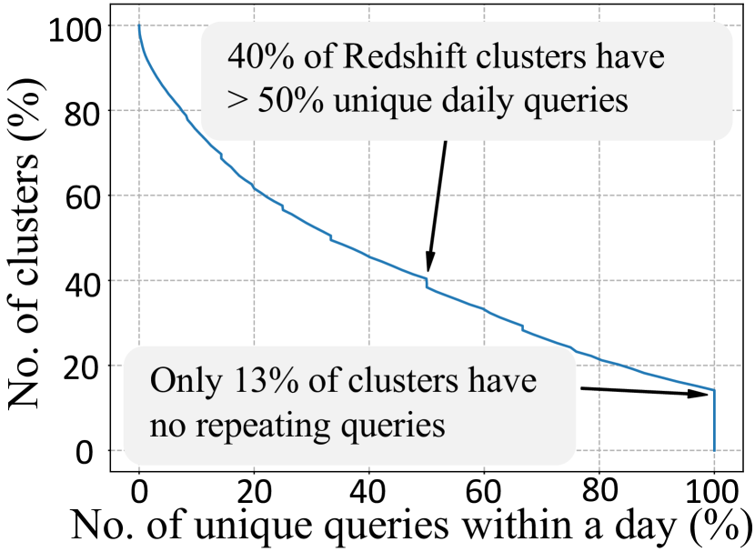
(a) Distribution of clusters by the % of queries that were unique within a day (not repeated).

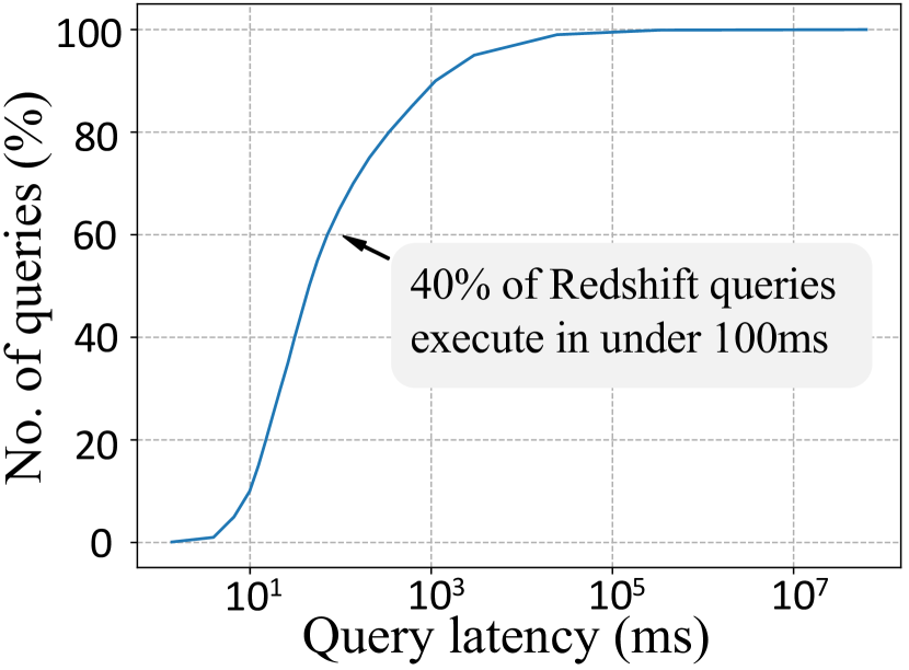
(b) Distribution of query latency across the Redshift fleet (0.01% to 99.99% shown).

Figure 1. Distribution statistics from the Redshift fleet

We make two key observations about the Amazon Redshift fleet that motivate the design of our new exec-time predictor. First, most queries executed on Amazon Redshift are low latency queries. Many queries execute in just a few milliseconds, so naively applying the advanced exec-time predictors in recent literature (Sun and Li, 2019; Marcus and Papaemmanouil, 2019; Hilprecht and Binnig, 2022), which have inference time on the order of 50ms to 500ms, on the critical path will result in more time being spent on prediction than on actual query execution. Thus, despite the superior estimation accuracy of these modern techniques, their inference latency overhead is not affordable for a lot of Redshift queries. For example, the predictor proposed in (Marcus and Papaemmanouil, 2019) has a prediction latency of 100ms, which is longer than $40\%$ of queries running in Redshift (as shown in Figure 1(b))! Second, Amazon Redshift customers tend to issue repeating queries. On average, more than $60\%$ of the queries executed within Amazon Redshift have been executed within 24 hours of the execution of an identical query (as shown in Figure 1(a)).

To address the challenges of cold-start prediction, inference time, and reliable estimation, we implemented a novel hierarchical exec-time predictor (Stage) with three stages of models illustrated in Figure 2: (1) a local exec-time cache, which simply memorizes the latency of recently executed queries and predicts that latency when the exact query is submitted again, (2) a local lightweight exec-time predictor with uncertainty measurement that is instance-optimized to each Redshift customer, and (3) a complex global predictor that is transferable across all instances in Redshift. When a new query $Q$ arrives, Stage predictor will first look up $Q$ in exec-time cache and directly return its prediction based on previously observed exec-time if $Q$ is present in the cache. If a query $Q$ misses the cache, Stage predictor will use a lightweight local exec-time predictor (local model) to predict its exec-time and an uncertainty measurement of the prediction. The local model utilizes a Bayesian ensemble of lightweight XGBoost models (Malinin et al., 2021) that can provide a query exec-time prediction and a reliable uncertainty measure associated with the prediction with a very low inference latency. While the local model never learns a fully generalizable model of query performance, it can accurately predict queries similar to the past-seen queries. Thus, it can be thought of as a “fuzzy cache”. The prediction uncertainty can be high whenever the local model does not have enough training examples, or the input query is very different from previously seen queries. In this situation, Stage predictor will use the global model. Inspired by the recent advance in zero-shot cost model (Hilprecht and Binnig, 2022), we design our global model as a graph neural network (Wu et al., 2022; Scarselli et al., 2008) that takes a physical execution plan of a query as input to predict its exec-time. There exist tens of thousands of instances in Redshift with diversified workloads. Thus, we train a single global model on a diverse set of instances to distill the transferable knowledge of exec-time prediction across various instances. As a result, it is capable of accurately and robustly predicting the exec-time of queries on unseen clusters. The global model will have a non-trivial inference latency (up to 100ms). Therefore, when used on a critical path of query execution, it will only be used when the local model is uncertain about its prediction and believes the query’s exec-time to be longer than a couple of seconds. Because the global model is rarely used, the additional inference overhead is amortized out.

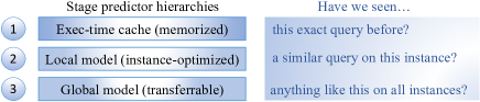
Figure 2. The key components and ideas of Stage predictor.

We simulate Stage predictor inside the workload manager (Saxena et al., 2023) of Amazon Redshift in an actual production environment. We conduct end-to-end evaluations on the 100 most billed instances in the month of July 2023 for each of three regions: ‘us-east-1’, ‘us-west-2’, and ‘eu-west-1’. The results show that Stage predictor can improve the average query execution latency by $20\%$ on these instances compared to the prior exec-time predictor in Redshift. In addition, we conduct thorough ablation studies to demonstrate the performance and reliability of each component of Stage predictor.

To the best of our knowledge, Stage predictor is the first to apply the idea of a hierarchy of models in exec-time prediction or similar tasks in DBMS. We believe that Stage predictor points out a way to practically integrate expensive machine learning models on the critical path of customer-facing production systems. We list the main contributions of this paper as follows:

• We describe the use cases and unique challenges of the exec-time predictor in Redshift (Section 2 and Section 3).

• We design a Stage predictor framework with hierarchical components for exec-time prediction (Section 4).

• We show a comprehensive evaluation of production data to showcase the advantages of Stage predictor (Section 5).

• We summarize the lessons learned and point out important research questions (Section 6).

2. Background

In this section, we first give an overview of query processing in Amazon Redshift, and then we provide a brief survey of related works on query exec-time prediction.

2.1. Execution time predictor in Redshift

Figure 3 illustrates the lifetime of user-issued queries inside Redshift. The queries will first go through a parser and query optimizer to derive their physical execution plans. Then, the exec-time predictor will take these plans as input and predict their exec-time. Based on their predictions, the workload manager will make a series of choices to determine their execution strategy and resource allocations (see (Saxena et al., 2023) for an overview). Finally, the workload manager will send the queries out for actual execution.

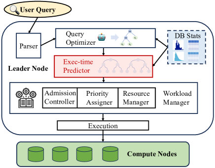
Figure 3. Queries’ lifetime inside Redshift.

Importance of exec-time predictor

The predicted exec-time is a critical component of the workload manager’s decision-making choices. Based on the prediction, the admission controller in the workload manager will decide whether a query should wait in the queue, be pushed to a special short query queue, be executed on the user’s main cluster, or be sent to a concurrency scaling cluster. For queries waiting in a queue, each query’s priority is determined by the predicted exec-time (short queries execute first). If the workload manager decides to start up a new concurrency scaling cluster to process an incoming query, the optimal cluster size will be chosen based on the predicted exec-time on the candidate cluster sizes. Therefore, the accuracy of exec-time predictor directly affects query performance in Redshift. For example, if exec-time predictor is inaccurate, it can mistake a long-running query as short-running. This long-running query can block the execution of other short-running queries in the queue, thus severely degrading the overall query latency. Conversely, if a shorting-running is mistaken as long-running, it may queue up for minutes before execution.

In addition to the usage of exec-time predictor on the critical path of query execution, it is also used in several other high-level optimization tasks. For example, automatic materialized view creation in Redshift (Armenatzoglou et al., 2022) uses the query optimizer to regenerate queries’ execution plans as if certain materialized view exists and then uses the exec-time predictor to estimate the performance of these plans to determine the benefits of building such materialized view.

The prior AutoWLM exec-time predictor in Redshift

Here, we summarize the current status of the exec-time predictor in Redshift as described in prior work (Saxena et al., 2023), the AutoWLM predictor. First, the AutoWLM predictor takes a physical execution plan of a query as input and flattens it into a vector. Then, a lightweight XGBoost model (Chen and Guestrin, 2016) is used to predict the query’s exec-time. As queries are executed in each instance, their feature vector and observed exec-time are added to the XGBoost model’s training set.

The AutoWLM predictor is lightweight to ensure negligible inference latency and memory overhead on the critical path of query execution. However, due to its lightweight nature and simplified query functionalization techniques, it can sometimes produce inaccurate estimations. Worse yet, some customers’ data and query workload change quickly, thus making the predictions unreliable. In addition, the AutoWLM predictor requires sufficient executed queries as training examples, which may not be available for a new instance (and hence a cold-start problem). Moreover, many downstream tasks require not just an estimate of exec-time but also a confidence interval around that estimate for robust optimizations. For example, the automatic materialized view creation and cluster scaling model in Redshift need a confidence interval to ensure good worst-case behavior of the changes in the cluster. The AutoWLM predictor provides these confidence intervals using simple global statistics, which leaves room for improvement.

2.2. Related Works

Here, we give a brief overview of previous results in the areas of uncertainty quantification and query performance prediction.

Uncertainty of XGBoost models

XGBoost is a scalable approach for building gradient boosting tree models, which achieved state-of-art performance in a wide range of tasks (Chen and Guestrin, 2016; Ogunleye and Wang, 2020; Zhang et al., 2018; Torlay et al., 2017). Recent work proposed a Bayesian ensemble of gradient boosting tree models to estimate the uncertainty of model prediction (Malinin et al., 2021). We abuse the term XGBoost models to refer to gradient-boosting tree models for easier understanding. In a nutshell, this approach separates the uncertainty into model and data uncertainty. It trains the XGBoost models with a probabilistic likelihood loss function (Prokhorenkova et al., 2018). Thereafter, instead of predicting a single name, the XGBoost models will output a mean $\mu$ and variance $\sigma$ for its prediction, where $\mu$ is the model prediction and $\sigma$ captures the data uncertainty. The Bayesian ensemble of XGBoost models independently trains several XGBoost models, denoted as $M_{1},\ldots,M_{k}$, each of which will produce a $\mu_{i}$ and $\sigma_{i}$. The variance of all output means $\mu_{1},\ldots,\mu_{k}$ captures the model uncertainty. Finally, the total uncertainty of prediction is the sum of model uncertainty and data uncertainty. Stage predictor adapts this approach to build an instance-optimized local predictor. The details will be discussed in Section 4.3.

Instance-optimized exec-time predictor

Traditional exec-time predictors generally use hand-derived heuristics and statistical models to understand the relational operators (Duggan et al., 2014; Wu et al., 2013; Akdere et al., 2012; Li et al., 2012). There has been a line of work using machine learning models to predict the exec-time of a query with superior accuracy over their traditional counterparts. In general, they featurize the logical or physical query plan as a graph and train graph neural networks to map the query plan to its exec-time (Marcus and Papaemmanouil, 2019; Sun and Li, 2019; Marcus et al., 2019, 2021; Yang et al., 2022; Zhou et al., 2020). One common drawback of these approaches is their high inference latency, preventing Redshift from integrating them on the critical path of query execution. Many Redshift queries execute in just a few milliseconds, and the inference latency of these methods surpasses a large proportion of queries’ actual execution time.

Zero-shot exec-time predictor

In contrast to instance-optimization, zero-shot exec-time predictor (Hilprecht and Binnig, 2022) proposed to train one model over a diverse set of DB instances, and it can be directly used to predict the query exec-time on arbitrary unseen DB instances. Specifically, the zero-shot model gathers data-specific statistics from each DB instance, such as the number of tuples/columns/pages of each table. Then, it embeds these statistics into a physical query execution plan to predict its exec-time. After a heavy offline training process, the zero-shot model understands the data-independent knowledge about the system and is transferrable to unseen DB instances. Stage predictor adapts this approach to build an instance-optimized global predictor inside Redshift. The details will be discussed in Section 4.4.

Machine Learning for Databases

In addition to exec-time prediction, machine learning has a large impact on optimizing and managing modern database systems. Machine learning systems help enable more effective and automated workload management (Marcus and Papaemmanouil, 2016; Saxena et al., 2023; Zhang et al., 2020), index recommendation (Ding et al., 2019), and configuration tuning (Aken et al., 2017). Machine learning algorithms help build more fine-grained and instance-optimized sub-components embedded in existing DBMSes, such cardinality estimation (Hilprecht et al., 2020; Yang et al., 2020; Zhu et al., 2021; Wu et al., 2023; Negi et al., 2023), learned query optimization (Marcus et al., 2019, 2021; Yang et al., 2022; Woltmann et al., 2023; Trummer et al., 2018), learned indexes (Kraska et al., 2018; Kipf et al., 2020; Nathan et al., 2020), and learned storage layouts (Ding et al., 2020; Curino et al., 2010).

3. Design Principles

Redshift’s query predictor has several design constraints, some likely to apply to other database engines, while others may be unique to Redshift. Here, we outline the three most important design principles behind our Stage exec-time predictor.

First, like many OLAP databases, a large number of queries seen by Redshift are repeated queries (e.g., dashboard refreshes) – taking advantage of this repetition is critical to correctly predicting latency for the majority of queries across the Redshift fleet. Second, standard point predictions (i.e., mean estimates) are insufficient for the predictor’s downstream tasks; we require reasonable confidence bounds around each prediction to guarantee worst-case performance. Third, the inference time of models on the critical path of query execution must be fast since a large portion of Redshift queries execute in only a few milliseconds. Thus, we set out to design a predictor with inference time on the order of microseconds.

Repeated queries

Many customers use Redshift for analytics tasks like dashboarding or report generation. As a result, identical queries are often repeatedly issued to Redshift. Figure 1(a) shows the distribution of the percentage of daily unique queries across the Redshift fleet: a “daily unique” query is a query sent to Redshift without an identical query being issued within the last 24 hours. Daily unique queries are thus a good lower bound for the number of repeating queries that Redshift sees, as monthly or weekly reports will not appear as daily unique queries. We observe that past performance of a query is a strong predictor of the same query’s performance later that day, since data distributions are normally static day-by-day (distribution shifts do occur, but normally not within 24 hours). Therefore, we want to design our predictor to take advantage of these repeating queries. This motivates the first “caching” stage of our predictive model, discussed in Section 4.2.

High-confidence predictions

Many off-the-shelf machine learning models (e.g., (Pedregosa et al., 2011)) give predictions as point estimates, or approximations of the mean. However, Redshift uses predictions in a number of downstream tasks, including query scheduling and cluster sizing, so error bounds are essential for ensuring the entire system maintains good worst-case behavior. Error bounds are especially important for deciding when to dedicate more inference time to make a more accurate prediction, which we discuss in Section 4.3.

Low inference latency

Since Redshift needs to estimate the exec-time for every issued query, it is important that the model’s inference procedure is efficient. Figure 1(b) shows the distribution of query latency across the Redshift fleet. Most Redshift queries execute in under $100ms$. This rules out exclusively using some modern advanced models, which could have inference times as high as $100ms$ (Marcus and Papaemmanouil, 2019; Sun and Li, 2019; Hilprecht and Binnig, 2022) (higher than the total query latency for 40% of the queries!). For Redshift, our new Stage predictor only uses an expensive neural network model when we have high confidence that a query will be long (details in Section 4.4). In this case, the additional inference time is a trivial portion of the overall exec-time.

4. Stage Predictor

In order to meet the specific needs of Redshift, we design the Stage exec-time predictor to work in stages. The first stage of the model, the exec-time cache (Section 4.2), remembers the recently executed queries. When an incoming query matches a past query, the exec-time cache makes a prediction. If a match is not found, the query proceeds to the next stage, the local model (Section 4.3). The local model is instance-optimized to each user’s clusters (i.e., trained per cluster). While the local model never learns a fully generalizable model of query performance, it can accurately predict queries that are slight modifications of past-seen queries. Thus, it can be thought of as a “fuzzy cache”. When it cannot make a confident prediction, the query proceeds to the final stage, the global model (Section 4.4). The global model is a state-of-the-art graph convolution neural network trained across the Redshift fleet.

4.1. Overview

Figure 4. Workflow overview of the Stage predictor: Queries are first planned by the query optimizer and then featurized into a vector. If the exec-time cache has a match for the feature vector, the cached exec-time will be returned. Otherwise, the feature vector will go to the local model. If the local model predicts that a query is short-running or if it is highly confident, its prediction will be returned. Otherwise, the global model will use the original physical plan and stats from the user’s specific database to make a prediction. After execution, the pair of vector representation and exec-time is added to the cache and local training data (not shown).

We present an overview of Stage predictor’s workflow in Figure 4. As discussed in Section 2, a user’s query $\mathcal{Q}$ will go through the parser and query optimizer to derive its physical execution plan before arriving at the exec-time predictor. Stage predictor first flattens the physical plan of $\mathcal{Q}$ into a 33-dimensional vector. The hashed vector is checked against the exec-time cache, which records the observed queries and their actual exec-time in the past. If $\mathcal{Q}$ is in the cache, we return the prediction based on its observed exec-time (within the Redshift, we find that $60\%$ of the queries will find a match in the cache). When $\mathcal{Q}$ misses the cache, we send $\mathcal{Q}$’s vector representation to the local model that is trained on executed queries on this instance, which will output a prediction and uncertainty associated with it. If the local model thinks that $\mathcal{Q}$ is short-running, or the local model is highly confident about its prediction, Stage predictor directly returns the local model’s prediction.

Finally, when the local model is uncertain about $\mathcal{Q}$, the state-of-the-art graph convolution neural network (global model) is used. The global model takes the physical plan of $\mathcal{Q}$ as input and understands the complicated interactions between operator nodes in this plan tree. A single global model is trained on all executed queries from a diverse set of instances and is shared across the entire Amazon Redshift fleet. As a result, the global model is more robust and accurate on the queries that the local model is uncertain about. The downside to the global model is that the global model has a high inference time (e.g., up to 100ms). However, since it is only used when local model is uncertain and thinks the query is long-running, it is rarely used, so the additional time is amortized out.

Advantages

The Stage predictor designs a systematic approach to use these models that best leverages the optimality (exec-time cache), instance-optimization (local model), and transferrable knowledge about Redshift (global model). By combining the merits of all these models with different characteristics, the Stage predictor is able to reliably achieve high prediction accuracy at a (amortized) negligible inference latency. Conceptually, the Stage predictor effectively addresses the downside of the prior AutoWLM predictor inside Redshift. In particular, the Stage predictor is able to significantly improve prediction accuracy without adding too much inference latency. In addition, the Stage predictor has reliable performance, especially when used on a new instance with insufficient training queries or instances with changing data and query workload. For those instances, the uncertainty of local model’s prediction will be high, and we can rely on the more robust global model. At last, the Stage predictor can provide probabilistic distribution or confidence interval for the predicted exec-time to enable robust decisions making of many downstream tasks.

4.2. Exec-time Cache

The exec-time cache is able to output near-optimal prediction with near-zero inference latency for repeating queries that were recently observed (this is $60\%$ of queries on average across the Redshift fleet). In the following, we first explain the cache’s keys and values, the procedure to make predictions, and the eviction policy of entries when the cache is full. Then, we discuss several optimizations.

Cache keys and values

Similar to AutoWLM predictor (Saxena et al., 2023), the first step of the Stage predictor is to flatten a physical plan tree as a vector. We traverse the plan tree, collect operator nodes of the same type, and sum up their estimated cost and cardinality. We also add features such as query type (e.g., SELECT, DELETE) and end up with an $n$-dimensional vector representation of the physical plan tree. The exec-time cache uses this vector for each query as key and maps the actual exec-time of this query after execution as values. For the same query that executes multiple times, the cache stores all their observed exec-times as values. It is worth noticing that in some very rare cases, two different plan trees may result in the same vector representation, which means that the exec-time cache cannot distinguish them. However, in those cases, their query plans should be very close to each other, and thus, we assume their exec-times should be similar as well.

Exec-time prediction

Whenever a new query arrives that matches a cached key, the exec-time cache is able to predict its exec-time based on its observed exec-times $t_{1},\ldots,t_{k}$. Since variance exists in these observed exec-times due to different system loads when the same query is being executed, one might think to use the mean $\mu$ of these exec-times as a prediction to increase prediction robustness. However, since the underlying table stats of Redshift may not be up-to-date, the same query executed at different time may access slightly different data, leading to different exec-times. In this case, $\mu$ will contain outdated exec-times, and the most recently observed exec-time $t_{k}$ captures the freshness of data. Therefore, we design a simple heuristic to predict the exec-time: $\mu\times\alpha+t_{k}\times(1-\alpha)$. This heuristic can capture both the robustness and the freshness of data. The value of $\alpha$ is a hyperparameter that balances the average exec-time against the most recently observed exec-time. Empirically, $\alpha=0.8$ works well for the Redshift fleet. In the future, we plan to design more principled approaches for prediction based on observed exec-time, such as time series prediction.

Eviction policy

In order to maintain efficient memory usage and fast look-up speed, we need to ensure the number of cached queries does not grow unbounded. Therefore, whenever the number of cached queries surpasses a certain threshold, exec-time cache will evict the least updated queries from the cache. In practice, this can be implemented by maintaining a sorted list of dates for each query at which the most recently observed exec-time is collected and removing the query with the oldest date from the exec-time cache.

Optimization 1: hash value replacement

As described above, the hash table stores query feature vectors as keys, so whenever an incoming query arrives, its entire query feature vector needs to be compared element-by-element with the cached vectors. We can optimize this vector-vector comparison by storing the hash value of the feature vector as the key. This, in theory, may lead to collisions, as any query feature vectors with matching hash values will be treated as identical, but we observed zero hash collision for all queries in the top 200 instances in the Amazon Redshift fleet. This optimization removes the costly vector-vector comparison and significantly reduces the size of the hash table keys.

Optimization 2: running mean and variance

As described above, the values in the hash table are lists of past query latencies. This gives us some design flexibility, as we can compute any summary statistic we want from the history (e.g., mean, median, quantiles). However, if we know we are only interested in the mean, variance, and the most recently observed exec-time, we can replace each query history with a running mean and variance. Using Welford’s algorithm (Welford, 1962), this only requires storing 4 values per hash table entry, reducing both the in-memory size of the cache and the cache’s lookup time (due to reading fewer in-memory values).

4.3. Instance-optimized local model

In this section, we first describe the implementation of our local model, and then conceptually justify the design choices for local model in Redshift and compare it with other potential alternative designs. At last, we explain how to leverage the exec-time cache to build an effective and efficient training pipeline for local model.

Bayesian ensemble of XGBoost models

As mentioned in Section 2.2, we adapt and implement the Bayesian ensemble of XGBoost models (Malinin et al., 2021) as our instance-optimized local model with a reliable uncertainty measurement. Recall that this ensemble independently learns $K$ XGBoost models, each of which takes the 33-dimension vector representation of query as input and estimates a mean $\mu_{k}$ and variance $\sigma^{2}_{k}$ of a query’s exec-time. The final prediction of exec-time $\hat{y}$ is given by the average of each model’s prediction in Equation 1. The total uncertainty $\mathcal{V}[\hat{y}]$ (i.e., variance of prediction) of this prediction $\hat{y}$ is a summation of estimated model uncertainty and estimated data uncertainty as shown in Equation 2.

(1) $$\hat{y}=\frac{1}{K}\sum_{k=1}^{K}\mu_{k}$$

(2) $$\underbrace{\mathcal{V}[\hat{y}]}_{\text{Prediction uncertainty}}=\ \ \underbrace{\frac{1}{K}\sum_{k=1}^{K}(\hat{y}-\mu_{k})^{2}}_{\text{Model uncertainty}}\ \ \ +\ \ \underbrace{\frac{1}{K}\sum_{k=1}^{K}\sigma^{2}_{k}}_{\text{Data uncertainty}}$$

Justification of the local model’s design choices

The model uncertainty is estimated as the variance of each XGBoost model’s prediction $\mu_{k}$. Since each model is independently trained, when local model does not have enough training data or if the incoming query is different from the training queries, the models will have diverse interpretations of this query. Thus, the variance of their prediction will be high in this scenario, and the global model could come to the rescue.

The estimated data uncertainty can capture the inherent noisiness in the labels and training features themselves. In Redshift, the same query executed at a different time can have different exec-times (i.e. noisiness in labels) due to different system loads and concurrency state. Meanwhile, the input to local model also contains high noise. Specifically, the 33-dimensional vector feature does not fully capture all information of the physical query plan tree (e.g., tree structure, missing node types, and Redshift’s cardinality estimation error). When a query plan is complicated with many joins, the vector feature tends to be less representative and the local model will have a high data uncertainty. In this case, the global model will take the entire physical execution plan as input and will have a better performance.

Therefore, using the Bayesian ensemble of XGBoost models as the local model captures two sources of uncertainty that could result in high prediction errors in Redshift. There exists a line of works in the machine learning domain for quantifying the prediction uncertainty, which are less optimal to apply inside Redshift. Specifically, uncertainty measurement using deep learning models (Gal and Ghahramani, 2016; Lakshminarayanan et al., 2017; Wilson and Izmailov, 2020) are not practical in Redshift due to their large inference latency. The popular lightweight alternatives for uncertainty measurement normally only focus on one source of uncertainty. For example, uncertainty in random forest regression (Mentch and Hooker, 2016; Coulston et al., 2016), quantile regression forests (Meinshausen, 2006), and one-class support vector machine for outlier detection (Li et al., 2003; Amer et al., 2013) mainly focus on quantifying the model uncertainty but not the data uncertainty. Whereas, another line of works on probabilistic prediction (Gneiting and Katzfuss, 2014; Nowotarski and Weron, 2018; Duan et al., 2020; Roberts, 1965) and probabilistic programming (Gordon et al., 2014; Bingham et al., 2019) mainly focus on understanding the uncertainty in data itself rather than quantifying the model uncertainty.

It is worth noting that using the Bayesian ensemble of XGBoost models as local model in Redshift also involves minimal engineering effort since the prior AutoWLM predictor inside Redshift already uses XGBoost. In order to build the new local model, we only need to change the loss function of the XGBoost model and independently train multiple such models.

Local model training optimization

The training process of the local model needs to maintain a diverse set of training queries to train effective local models. At the same time, it also needs to ensure a low memory and computation overhead of training because the training process is conducted locally on the customers’ database clusters. Therefore, we tailor the training process based on the unique characteristics of Redshift queries.

We collect the observed features and latency of executed queries into a training query pool. Naively storing every query execution result in the training pool has the following three issues: (1) the size of the training pool would grow unbounded, (2) the training pool would become “polluted” with repetitive queries that the exec-time cache will take care of anyway, and (3) the training pool will have more short queries than long queries, skewing prediction accuracy for longer (and often more important) queries.

Bounding the size

To resolve the first issue of the training pool, we cap the total number of queries in the training query pool. Whenever the number of queries exceeds a certain threshold, the training pool will evict the oldest observed queries.

Dealing with repeats

Recall that a large amount of queries in Redshift repeat themselves, which will significantly reduce the diversity of queries in the training pool. Besides, these repeating queries will be captured by the exec-time cache, so overfitting these queries may degrade local model’s generalizability to other queries. Therefore, we deduplicate the repeating queries in the training pool. We leverage the exec-time cache to implement this data deduplication efficiently. Specifically, for each executed query, we hash its observed features and check against the exec-time cache. If the query misses the cache, we add it to the training pool.

Duration diversity

Next we address the third issue, which is that the distribution of query latencies is skewed. Most of the Redshift queries execute in less than a couple of seconds, so our training pool can be filled by short-running queries. In this case, the local model will have catastrophic performance for longer-running queries. Therefore, we partition the training pool into several query exec-time buckets (e.g., $0-10s$, $10-60s$, and $60s+$) and assign a cap for each bucket to ensure the query diversity in the training pool.

4.4. Transferrable global model

Inspired by recent work in zero-shot cost model (Hilprecht and Binnig, 2022), we design the instance-independent featurization of Redshift query plans, allowing us to map query plans from various customers’ instances to a unified space. As a result, we can collect a diverse set of training queries from a large amount of Redshift instances to jointly train one global model that is able to make robust predictions for all instances, including the unseen instances. The global model uses a graph convolutional network (GCN) (Kipf and Welling, 2016) architecture to understand the query plan of Redshift and map it to its exec-time.

Figure 5. Global model featurization and architecture.

Query plan featurization

We run the fleet sweep to gather the logs (i.e., STL_EXPLAIN table) on the physical execution plans of executed queries from the customers’ Redshift instances. Then, we parse the information from the logs into a tree data structure representing each query plan as shown in Figure 5. Each node in the tree represents a physical operator (e.g., “sequential scan”, “hash”, “materialize”, “distributed hash join”, “aggregate”, “order by”), and we featurize it as its operator type, estimated cost, estimated cardinality, tuple width, S3 table format (e.g., “Parquet”, “OpenCSV”, “Text” or “Local” if the table is stored locally), and number of rows in the table. An example of node features is shown in red in Figure 5. It is worth noticing that 90 unique operator types exist in Redshift, so we represent the node operator type as a $90$-bit one-hot vector. Furthermore, we set the S3 table format and table rows features to “Null” if the operator is not directly operating on a base table (e.g., not a scan operation).

Model architecture

Our global exec-time predictor contains three components: node embedding, graph convolution message passing, and final exec-time prediction. First, the features of all nodes are embedded with a multi-layer perceptron (MLP) to a feature vector. One example is shown in blue color in Figure 5. Then, we use a GCN model to perform message passing between nodes to aggregate information and understand operator interactions in Redshift. Some message passing directions are shown in green in Figure 5. Specifically, GCN consists of several layers of message passing. In the first layer of GCN, each node combines its own embedded node features with those of its children and transforms them into a new node feature. This feature combination process is controlled by learnable weights. The following GCN layers will repeat the same process on the transformed features of each node from the previous layer. After several GCN layers, information on all nodes will be aggregated to the root node, and a vector representation of the entire query plan will be outputted. The GCN message passing is capable of understanding the complex operator dependencies and interactions, as shown by the zero-shot cost model (Hilprecht and Binnig, 2022). At last, the final vector representation output by GCN will be concatenated with a system feature vector, which includes a summarization of the query plan, Redshift instance type, number of Redshift nodes, memory size, and number of concurrent queries. The system feature vector contains factors that may affect query exec-time other than the query execution plan itself. The concatenated feature will be sent to an MLP to estimate the exec-time of this query.

Our global GCN model is trained on a diverse set of hundreds of Redshift instances, each with more than 10,000 queries.

5. Experimental Evaluation

In this section, we evaluate the performance of the Stage predictor and compare it against the prior AutoWLM predictor in Redshift on real-world data. We first explain the experimental setting in Section 5.1 and then evaluate the following questions:

• End-to-end (Section 5.2): How much practical gain can the Stage predictor achieve in terms of improving end-to-end query execution latency in Redshift?

• Accuracy (Section 5.3): How accurate is the Stage predictor? What is its model size and inference latency?

• Ablation (Section 5.4): How accurate and robust is each hierarchy of Stage predictor individually?

5.1. Experimental Settings

Real-world workloads

Since we are primarily concerned with the performance of the Stage predictor on the Redshift fleet, we evaluate the Stage predictor on query logs of real Redshift customers. We select the top 100 most-billed instances in the month of July 2023 from Redshift in each of the three regions: ‘us-east-1’, ‘us-west-2’, and ‘eu-west-1’. We select all user-executed queries on these instances from ‘July 28th, 2023’ to ‘August 11th, 2023’, resulting in a total of roughly 30 million queries. Unless specifically stated otherwise, all our experiments are conducted on these queries.

Local environment

We train and evaluate the performance of our Stage predictor and the baseline (i.e., AutoWLM predictor in Redshift) on one AWS ‘m5.4xlarge’ machine with 64 GB memory, 16 vCPUs, and Intel Xeon Platinum 8175 processor. It is worth noting that the offline training of our global model is conducted on two AWS ‘p3.8xlarge’ machines, each with 244 GB memory, 32 vCPUs, and 4 Nvidia tesla v100 GPU. We only leverage GPU to accelerate the training of the global model, not the cache or local model.

Model training

We simulate the exact training and testing procedure as in real Redshift deployment to evaluate the performance of Stage predictor and the baseline. Specifically, on each cluster, we replay all the queries sequentially based on their logged execution start time. In addition, we randomly sample 100 training instances and use three weeks of user-executed queries on all instances to train our global model. These training instances do not overlap with the evaluation instances. Unless specified otherwise, all predictions used for evaluation are derived from the aforementioned procedure.

Hyper-parameters

Our Stage predictor contains a set of hyper-parameters that are relatively easy to tune. We describe each of the hyper-parameters and its value as follows. Each value was determined via tuning on data prior to our test workload (i.e., data used to select hyperparameters is completely separate from the evaluation dataset). For the exec-time cache, we set the cache size to 2,000 (i.e., it can only keep 2,000 unique queries before eviction). For the local model, we used the CatBoost Python package (Prokhorenkova et al., 2018) to train $10$ XGBoost models independently. For each XGBoost model, we set the number of estimators as 200, the max depth as 6, and the number of parallel trees as 1. When training the XGBoost models, we randomly choose $20\%$ of the training data as a validation set for early stopping to prevent overfitting. We note that the AutoWLM predictor baseline in Redshift uses exactly the same hyperparameters for the XGBoost model. The differences between our local model and the baseline are (1) we train 10 models instead of one; (2) we use a log-likelihood loss function instead of the mean absolute error as used by the baseline. Both changes are necessary to provide an uncertainty measure of prediction. For global model, we use a directed GCN with the hidden dimension size 512, 8 layers of graph convolution, and $0.2$ weight dropout ratio.

5.2. End-to-end Evaluation in Redshift

The most straightforward and important approach to evaluate the effectiveness of Stage predictor is to test how much it can improve the end-to-end query execution latency inside Redshift. It is worth noticing that query latency is different from query exec-time — latency includes the scheduling time and wait time of a query, whereas exec-time excludes those factors.

End-to-end simulation

To evaluate the impact of the Stage predictor on end-to-end performance, we simulate the Redshift workload manager (Saxena et al., 2023) using the Redshift team’s internal tools. The simulator replays an existing user workload using the Stage predictor. The simulator then computes the expected query latency of each query in the workload. More accurate exec-time predictions will cause the workload manager to make better scheduling decisions and thus improve query latency. It is worth noticing that in this simulation, exec-time prediction accuracy only affects query wait time but not actual query exec-time: that is, the query execution time is assumed to be identical to when the query was actually executed by the customer. This could lead to some simulation inaccuracies since the workload manager’s decisions can impact query execution time (i.e., resource allocation). However, we have verified through various other experiments conducted internally by Redshift teams on the workload manager that improvements in the simulation results accurately reflect actual query execution latency in production.

We chose the workload manager simulation as our end-to-end evaluation for two reasons. First, we cannot directly compare the Stage predictor with the AutoWLM predictor in real production environments. This is because users execute their queries once and once only, so the workload manager either uses the Stage predictor or the AutoWLM predictor to get the actual query execution latency. Counterfactually “replaying” the workload via a simulator is the only way to measure possible improvements. Second, other tasks exist in Redshift as sub-routines (e.g., automatic materialized view creation). However, those tasks are not on the critical path of query execution, so they can only indirectly reflect the query execution latency changes. Thus, we cannot explicitly evaluate the benefit of Stage predictor on those tasks. It is worth noticing that part of the Stage predictor (exec-time cache and local model) is already deployed in production. Due to some observed regression in the accuracy of global model (see Section 5.4), we are exploring a more robust global model before deploying it in Redshift.

Figure 6. End-to-end performance in terms of query latency of different exec-time predictors inside Redshift. We listed the percentage improvement over the AutoWLM predictor.

Performance comparison

We conduct the simulation experiment using three exec-time predictors: Stage predictor, the AutoWLM predictor, and the actual exec-time (Optimal). The Optimal feeds the observed exec-time to the workload manager, representing the optimal performance an exec-time predictor can ever achieve.

The overall end-to-end query execution latency on all top 100 most-billed instances in three regions (roughly 30 million queries) are shown in Figure 6. We observe that the Stage predictor significantly improves over the AutoWLM predictor: the $20.3\%$, $16.4\%$, and $14.9\%$ query execution latency improvement on average, median, and tail, respectively. This improvement purely results from a more accurate exec-time predictor. However, we observe that Optimal has a significantly better performance than Stage predictor: $44.4\%$, $59.8\%$, and $54.5\%$ query execution latency improvement on average, median, and tail, respectively. This suggests that there still exists a large room for improvement, and further improving the accuracy of exec-time predictor in Redshift can be fruitful.

Figure 7. End-to-end query latency improvement over AutoWLM predictor on each top instance. We sort the instances based on the improvement the optimal predictor achieves.

In addition, we analyze the average query latency improvement of the Stage predictor over the AutoWLM predictor on each instance in Figure 7. For comparison, we also plot the optimal predictor’s improvement and sort the instances based on this value. We can see that the Stage predictor is able to improve the average query latency for most of the instances. However, there are regressions: on less than $10\%$ of the instances, Stage predictor actually does worse than the AutoWLM predictor. There are several possible explanations. First, the AutoWLM predictor does occasionally make better predictions than the Stage predictor on a small portion of queries, which could have an impact on the workload manager. Second, both the Stage predictor and the AutoWLM predictor have erroneous predictions, as detailed in Section 5.3, and there is an asymmetry in prediction errors. For example, for a query with exec-time of 30s, the Stage predictor may predict it to be 5s, thus sending it to the short-running queue, and the AutoWLM predictor may make a worse prediction of 900s, thus sending it correctly to the long-running queue. In this scenario, although Stage predictor is more accurate, it makes the wrong decision. Third, due to the algorithmic design of workload manager (Saxena et al., 2023), there will be edge cases when perfect prediction does not lead to the best end-to-end query latency. This also explains why the Stage predictor can sometimes outperform the optimal predictor.

5.3. Stage Predictor Accuracy

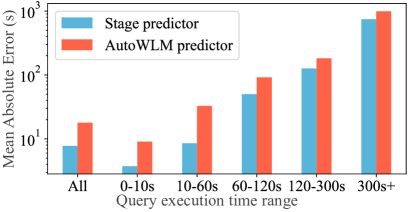
Figure 8. Prediction accuracy of stage predictor compared to the AutoWLM predictor in Redshift.

We show the prediction accuracy of the Stage predictor and the AutoWLM predictor on all top 100 most billed instances from three regions in Redshift, with a total of $27,441,359$ queries. The accuracy is evaluated using absolute error, that is, —actual exec-time $-$ predicted exec-time— in seconds. We show the accuracy comparison in Figure 8 and report the details of mean (MAE), median (p50-AE), and tail (p90-AE) absolute error of these queries in Table 1. Stage predictor is able to achieve a median absolute error of $0.67$, suggesting that for $50\%$ of the query, Stage prediction is within $0.67s$ of actual execution time. Overall, Stage predictor achieves more than 2x more accurate prediction than the AutoWLM predictor.

Query Exec-time	# Queries	Stage predictor			AutoWLM predictor
		MAE	P50-AE	P90-AE	MAE	P50-AE	P90-AE
Overall	27,441,359	7.76	0.67	9.39	17.87	2.03	23.68
0s – 10s	22,015,851	3.74	0.31	7.43	9.04	1.11	14.44
10s – 60s	5,085,965	8.53	2.60	13.68	32.83	10.02	51.34
60s – 120s	163,913	50.11	24.15	85.00	91.63	31.04	113.8
120s – 300s	83,590	126.4	70.46	206.4	181.9	84.55	255.4
300s+	92,041	744.4	235.7	1496	990.1	289.7	1922

Table 1. Prediction accuracy (absolute error in seconds) of stage predictor and the AutoWLM predictor.

Query Exec-time	# Queries	Stage predictor			AutoWLM predictor
		MQE	P50-QE	P90-QE	MQE	P50-QE	P90-QE
Overall	27,441,359	54.57	1.60	19.00	171.8	4.08	135.7
0s – 10s	22,015,851	43.87	1.92	26.25	97.41	6.38	173.1
10s – 60s	5,085,965	71.66	1.18	2.16	441.4	1.77	6.39
60s – 120s	163,913	251.9	1.38	4.57	633.2	1.51	4.97
120s – 300s	83,590	307.4	1.59	5.83	548.1	1.71	6.61
300s+	92,041	1084	1.48	6.12	1922	1.58	10.00

Table 2. Prediction accuracy (in Q-error) of stage predictor compared to the AutoWLM predictor.

To dive deep into the results, we provide a detailed accuracy comparison on queries with different exec-time ranges in Table 1. It is very important to analyze the prediction performance of queries with different exec-time ranges because the workload manager of Redshift schedules queries into execution queues and assigns priority according to the predicted exec-time. Specifically, we see that Stage predictor is able to achieve more than $3x$ better prediction on queries with less than 60s exec-time. We additionally provide the same table on another widely-used metric for relative error: Q-Error (Moerkotte et al., 2009), that is, $max\{predicted/true,true/predicted\}$ in Table 2. The minimal value Q-Error can take is 1, and closer to 1 implies a more accurate prediction. We observe a roughly similar pattern that the Stage predictor significantly outperforms the AutoWLM predictor on 60s exec-time. However, it achieves mild improvement on the queries with more than 60s exec-time, possibly due to the following reasons. First, the distribution of query exec-time is heavily skewed and only $1\%$ of the queries execute longer than 60s. Therefore, both Stage predictor and the AutoWLM predictor don’t have enough training data on the long-running queries and yield worse performance. Second, the long-running queries are inherently more difficult to predict because of a larger noisiness in the label. We observe in Redshift that the exec-time of the same query repeatedly executed several times can range from just tens of seconds to several hundred seconds. This scenario is largely due to different system loads, cache states, and the number of concurrency queries in Redshift during the query execution. Unfortunately, our exec-time predictor cannot yet take that into account. In future work, we plan to design better exec-time predictors that can take system statistics into account to explain the variance in labels.

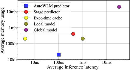
Figure 9. Average inference latency and average memory usage overhead of different exec-time predictors.

In addition to accuracy, we provide the average inference latency and memory usage overhead of Stage and AutoWLM predictor along with each component of Stage predictor in Figure 9. It is worth noticing that since different instances of Redshift are likely to have different hardware types, the numbers in Figure 9 are rough estimations rather than actually measured inference latency and memory usage. Although Stage predictor (red dot) has a larger inference latency and memory overhead than the AutoWLM predictor (blue square), it is still within a practical range: sub-millisecond inference latency, a few hundred kb memory usages. Specifically, the exec-time cache (yellow dot) is able to make an inference in just a couple of microseconds. The local model (green dot) trains $10$ XGBoost models as opposed to one in AutoWLM predictor, so it is generally $10x$ larger and slower to make inferences than AutoWLM predictor. The global model (purple dot) is a deep-learning-based model, which is roughly two of a magnitude larger than other predictors. However, since the deep learning model is rarely used ($3\%$ of the time), its inference latency is amortized out. Furthermore, we do not include the memory overhead of global model into Stage predictor because it will eventually be deployed as a serverless Lambda function that every Redshift instance can invoke to avoid local memory and CPU overhead.

5.4. Ablation study

In this section, we first provide detailed accuracy analysis on each component of Stage predictor: exec-time cache, local model, and global model. Then, we study how reliable is the uncertainty measure of our local model.

Accuracy of exec-time cache

Query Exec-time	# Queries	Exec-time cache			AutoWLM predictor
		MAE	P50-AE	P90-AE	MAE	P50-AE	P90-AE
Overall	16,963,658	4.83	0.56	4.66	15.04	3.00	20.35
0s – 10s	12,616,915	1.82	0.16	2.74	7.40	1.20	15.96
10s – 60s	4,212,128	4.55	2.27	6.61	23.15	7.57	24.26
60s – 120s	74,604	30.87	9.80	67.93	43.88	23.29	77.2
120s – 300s	27,185	115.8	72.78	197.8	117.4	88.13	205.6
300s+	32,826	764.3	193.4	1524	1046	284.4	2045

Table 3. Prediction accuracy (absolute error in seconds) of exec-time cache and AutoWLM predictor in Redshift.

We find that $16,963,658$ out of the $27,441,359$ queries in these instances ($61.8\%$) repeat themselves and can be directly predicted by exec-time cache. As shown in Table 3, exec-time cache overall achieves a significantly better prediction accuracy than the AutoWLM predictor. The advantages are apparent since the AutoWLM predictor (XGBoost model) is trained on the executed queries’ exec-time as ground truth, which is captured in the cache. Therefore, in theory, the locally trained model can never outperform the exec-time cache. However, it is worth noticing that exec-time cache does make significant errors (in terms of absolute error) because these repeating queries are executed at different system loads, buffer pool states, and concurrency conditions, making it extremely hard to predict the exec-time at a different state accurately. We find roughly the same pattern for prediction accuracy comparison in terms of Q-error, so we omit all results on Q-error due to space limitations.

Query Exec-time	# Queries	Local model			AutoWLM predictor
		MAE	P50-AE	P90-AE	MAE	P50-AE	P90-AE
Overall	10,477,701	21.48	4.16	34.88	19.06	4.32	29.27
0s – 10s	9,398,936	13.76	3.27	30.88	10.94	3.60	23.41
10s – 60s	873,837	35.63	16.47	87.06	32.63	12.90	54.36
60s – 120s	89,309	77.69	37.61	137.6	69.65	36.04	93.40
120s – 300s	56,405	140.1	72.03	230.5	120.7	76.75	195.1
300s+	59,215	840.3	267.6	1652	852.3	276.0	1729

Table 4. Prediction accuracy (absolute error in seconds) of the local model and AutoWLM predictor in Redshift.

Accuracy of local model

We evaluate and compare the performance of the local model to the AutoWLM predictor in Redshift on the $10,477,701$ out of the $27,441,359$ queries that miss the exec-time cache ($38.2\%$). Recall that there are only two differences between local model and AutoWLM predictor: 1) local model independently trains $10$ XGBoost model whereas AutoWLM predictor only uses one; 2) the XGBoost model in local model is trained with log-likelihood loss whereas AutoWLM predictor is trained with the absolute error. We observe in Table 4 that local model is slightly worse than the AutoWLM predictor because the AutoWLM predictor is directly trained to optimize the absolute error, which is the evaluation metric. As a future work, we plan to lower the gap in performance difference between the two by adding an XGBoost model trained with absolute error into the Bayesian ensemble of XGBoost models in local model.

Accuracy of global model

The global model is trained on a diverse set of instances and evaluated on the top-billed instances with unseen queries. We first compare the performance of global model against the local model on all queries that miss the cache in Table 5. We observe that the local model has a better performance than global model, especially on long-running queries. This was surprising to us because it runs against the common wisdom that “more data makes a better model”: in this case, the global model is trained on significantly more data than the local model. However, the local model’s data is much closer in distribution to the test data, and the local model is able to win out. While there are some specific databases where the global model outperforms the local model, the overall trend favors the local model, which might be evidence that, in the context of query performance prediction, better data beats bigger data. In our opinion, this casts serious doubt on the premise that cloud database operators can train effective “cross-customer” models that are better than instance-optimized models.

Query Exec-time	# Queries	Global model			Local model
		MAE	P50-AE	P90-AE	MAE	P50-AE	P90-AE
Overall	10,477,701	23.82	6.42	29.53	21.48	4.16	34.88
0s – 10s	9,398,936	12.61	8.48	20.96	13.76	3.27	30.88
10s – 60s	873,837	39.42	17.92	67.58	35.63	16.47	87.06
60s – 120s	89,309	166.1	111.9	204.6	77.69	37.61	137.6
120s – 300s	56,405	366.5	243.9	519.9	140.1	72.03	230.5
300s+	59,215	1763	701.5	3540	840.3	267.6	1652

Table 5. Prediction accuracy (absolute error in seconds) of the global model compared to the local model on all queries that miss the exec-time cache.

Query Exec-time	# Queries	Global model			Local model
		MAE	P50-AE	P90-AE	MAE	P50-AE	P90-AE
Overall	361,752	134.8	10.09	164.1	164.7	25.21	196.8
0s – 10s	167,617	9.45	3.90	20.37	50.77	18.82	113.4
10s – 60s	91,714	33.31	48.46	67.58	62.12	20.14	113.0
60s – 120s	37,539	64.72	35.78	92.89	82.03	34.27	151.2
120s – 300s	31,508	230.7	90.51	309.9	235.5	82.14	326.6
300s+	33,343	1033	423.8	2011	1046	391.9	1712

Table 6. Prediction accuracy (absolute error in seconds) of global model compared to local model on uncertain queries.

One possible explanation for the relatively poor performance of the global model is a lack of model capacity: could a sufficiently large model learn the latent information hidden in each database instance with enough training data? While we are unable to answer this question conclusively, we did find several examples of nearly identical query plans with nearly identical cost and cardinality estimates from different customers with drastically different performances. No amount of data can resolve this issue, as there are two nearly identical training inputs with wildly different desired outputs. Thus, database-specific features may be needed for a global model to learn to differentiate between these pairs.

For the context of this work, we primarily care about the performance of the global model when the local model is uncertain and thinks the query is long-running. We evaluate those queries in Table 6. In this scenario, global model is able to achieve a better result than the local model. This suggests that global model is able to provide more robust and reliable prediction whenever the local model is uncertain. However, we barely observe improvement on long-running queries (larger than 120s) over local model because those queries are very sparse in each instance and may contain instance-specific characteristics that the global model cannot understand. Overall, we do see a significant performance drop for local model itself, shifting from testing on all queries to only uncertain ones. This implies that our uncertainty measurement for local model is reliable. We provide a more exhaustive analysis of the reliability of this uncertainty measurement as follows.

Uncertainty measurement in local model

We use the well-established scoring rule: prediction-rejection ratio (PRR) (Malinin et al., 2021, 2020) to evaluate how good is the uncertainty measurement of local model. PRR quantifies the rank correlation between the predicted uncertainty and the observed prediction error for each query in one instance. To better explain how PRR works, we provide an example in Figure 10. On the left of Figure 10, we show 2000 testing queries from one instance and plot their uncertainty estimated by the local model on the x-axis against the observed absolute estimation error on the y-axis. We can see a statistically significant positive relation between these two values. On the right of Figure 10, we show the calculation of PRR for this instance. Specifically, we first sort/rank all queries based on their observed absolute estimation error (“Oracle”) in descending order and plot the proportion of cumulative error (i.e., cumulative error/total error) as shown in the red curve in this figure. Then, we sort/rank all queries based on their prediction uncertainty in the blue curve and randomly sort all queries as in the black curve. Ideally, if our uncertainty has a perfect correlation with the actual error, the blue curve should overlap with the red curve. Therefore, the “closer” blue curve is to the red curve, the more reliable our prediction uncertainty is. We can compute the area under the curve (AUC) between red and black curves as (AUC_Oracle) and the AUC between blue and black curves as (AUC_Stage). The PRR score is quantitatively defined as the ratio AUC_Stage/AUC_Oracle, between 0 and 1.

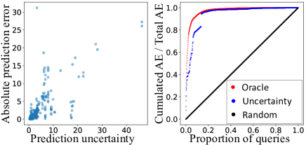
Figure 10. Illustration of PRR calculation on queries from an example instance, whose PPR score is 0.9.

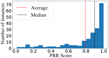
Figure 11. Uncertainty quality of local model (prediction rejection ratio) distribution for all top instances.

We calculate the overall PRR score for all top instances and plot their distribution in Figure 11. We can see that $30\%$ of the instance has a PRR score close to 1, which suggests that our uncertainty measurement can perfectly capture estimation error for these instances. We have a median PRR score of $0.9$, which is the same as the example in Figure 10. However, in some instances, the PRR score is very low, generally because of insufficient training queries.

6. Lessons learned and potential future research directions

Throughout the process of building Stage predictor in Redshift, we learned several important lessons that could benefit the research community. In the following, we describe these lessons and list potential research directions that could be valuable to the industry.

6.1. Applying Stage predictor in other tasks

Apart from improving the workload manager in Redshift, we believe the Stage predictor enables new solutions for many tasks in smart DBMSes, including query optimization and hypothetical reasoning.

Query optimization

Recently, many ML-based solutions have been proposed for query optimization (Marcus et al., 2019; Yang et al., 2022). Although these ML-based techniques can select join-order and physical operators more accurately than the traditional optimizers, their inference latency can get up to several hundred milliseconds. Thus, this overhead will be impractical to optimize short-running queries. To practically integrate ML-based optimizers into real systems, they can use Stage predictor as a sub-routine. Specifically, a query could first be optimized by the default query optimizer inside a system. Then, the query plan is fed into Stage predictor to estimate its exec-time, and the system will use the expensive ML-based optimizer to re-optimize the plan only if it is long-running.

Answering “what-if” questions

Hypothetical reasoning is a crucial element of many database decision-making tasks, including provenance updates, view manipulation, knob tuning, and automatic cluster scaling (Arab and Glavic, 2017; Nieva et al., 2020; Meliou and Suciu, 2012). Hypothetical reasoning allows DB administrators and users to test database assumptions by asking “what-if” questions, such as “what will the performance of existing queries be if an index on column X is created?”, “what if the data size increases by 5x?”, “what if the cluster adds 3 nodes?”. Answering “what-if” questions is very difficult. For example, learning a query performance predictor on the executed workloads of a database cannot accurately estimate the performance under “what-if” scenarios because the model does not observe any training data under such hypothetical scenarios. Therefore, existing methods mainly rely on casual inference to answer these questions (Meliou et al., 2010; Galhotra et al., 2022). In theory, the global model of Stage predictor could provide more accurate and more fine-grained answers to these “what-if” questions. Since the transferrable global model distills the knowledge of a DBMS, it will observe these “what-if” scenarios happening on other similar databases. Thus, it can leverage the observation on other databases to accurately predict the query performance under “what-if” scenarios of the current database.

6.2. Hierarchical models

When designing a practical exec-time predictor for Redshift, we found that although a plethora of ML-based predictors can provide more accurate exec-time prediction, their inference overhead is too large to be deployed on the critical path of Redshift. We believe this problem generally exists in the database research community beyond exec-time prediction and Redshift.

Most ML models naturally present a trade-off between accuracy and model size/inference latency that more accurate models tend to be more expensive. Thus, when sophisticated ML-based solutions are adopted to solve existing database problems on the critical path of query execution, they will inevitably incur a non-trivial overhead. This overhead may be unaffordable for short-running queries. We believe the hierarchical model solutions, similar to the Stage predictor, could enable a practical adoption of ML-based solutions to best leverage their accuracy with an affordable inference overhead. To the best of our knowledge, there does not exist other works in the database community that use the idea of hierarchical models. In the following, we provide a detailed example of cardinality estimation, which is on the critical path of query execution.

Cardinality estimation is crucial for query optimization. Due to its challenging nature, sophisticated ML-based solutions (Zhu et al., 2021; Hilprecht et al., 2020; Yang et al., 2020) have been proposed to improve the accuracy of their traditional counterpart. Their inference latency varies from a couple of milliseconds to a hundred milliseconds (Han et al., 2021), which will not be affordable for short-running queries. A hierarchy of several cardinality estimators with different accuracy/overhead trade-offs could enable practical integration of ML-based solutions in real systems. Specifically, the queries will first be fed into cheap estimators and more expensive estimators will be invoked only if the previous cheaper estimator is uncertain about its prediction. Therefore, the inference overhead of the expensive estimators can be amortized out.

6.3. Environment factors in exec-time prediction

Inside Redshift, we found that the same query in the same cluster can sometimes have very different exec-times ranging from a couple of seconds to several minutes, even hours because of different environment factors at the time of execution. These factors include memory and CPU utilizations that directly affect the query exec-time. For example, if $90\%$ of memory has been used by other jobs in the clusters, a query may spill its intermediate results to disk, incurring a large additional cost. However, simply adding the memory and CPU utilizations at the time of execution into the feature of predictor is unlikely to provide better prediction because they can vary throughout the execution of a query.

Furthermore, there exist other environment factors, such as cache effect and buffer pool state that are not trivial to featurize in Stage predictor or any other exec-time predictors. Specifically, the recently accessed pages will be cached which can greatly speed up the following queries touching the same pages.

We believe designing exec-time predictors that can accurately take these environment factors into consideration can further improve the prediction accuracy.

7. Conclusions

We have presented Stage, a novel hierarchical query performance predictor custom-tailored to Amazon Redshift’s specific requirements. The Stage predictor provides fast and robust query performance predictions by taking advantage of the repetitive nature of analytic workloads, remembering the latency of common, frequently-issued queries, and using two different machine learning models for similar and novel queries, respectively. We showed that Stage predictor improves the average query latency by 20% when compared to Redshift’s prior exec-time predictor. Based on the lessons learned from building Stage predictor, we pointed out a list of research directions that could be fruitful.

References

- (1)
- Akdere et al. (2012) Mert Akdere, Ugur Çetintemel, Matteo Riondato, Eli Upfal, and Stanley B. Zdonik. 2012. Learning-based Query Performance Modeling and Prediction. In IEEE 28th International Conference on Data Engineering (ICDE 2012), Washington, DC, USA (Arlington, Virginia), 1-5 April, 2012, Anastasios Kementsietsidis and Marcos Antonio Vaz Salles (Eds.). IEEE Computer Society, 390–401. https://doi.org/10.1109/ICDE.2012.64
- Aken et al. (2017) Dana Van Aken, Andrew Pavlo, Geoffrey J. Gordon, and Bohan Zhang. 2017. Automatic Database Management System Tuning Through Large-scale Machine Learning. In Proceedings of the 2017 ACM International Conference on Management of Data, SIGMOD Conference 2017, Chicago, IL, USA, May 14-19, 2017, Semih Salihoglu, Wenchao Zhou, Rada Chirkova, Jun Yang, and Dan Suciu (Eds.). ACM, 1009–1024. https://doi.org/10.1145/3035918.3064029
- Amer et al. (2013) Mennatallah Amer, Markus Goldstein, and Slim Abdennadher. 2013. Enhancing one-class support vector machines for unsupervised anomaly detection. In Proceedings of the ACM SIGKDD workshop on outlier detection and description. 8–15.
- Arab and Glavic (2017) Bahareh Sadat Arab and Boris Glavic. 2017. Answering Historical What-if Queries with Provenance, Reenactment, and Symbolic Execution. In 9th USENIX Workshop on the Theory and Practice of Provenance, TaPP 2017, Seattle, WA, USA, June 23, 2017, Adam Bates and Bill Howe (Eds.). USENIX Association. https://www.usenix.org/conference/tapp17/workshop-program/presentation/arab
- Armenatzoglou et al. (2022) Nikos Armenatzoglou, Sanuj Basu, Naga Bhanoori, Mengchu Cai, Naresh Chainani, Kiran Chinta, Venkatraman Govindaraju, Todd J. Green, Monish Gupta, Sebastian Hillig, Eric Hotinger, Yan Leshinksy, Jintian Liang, Michael McCreedy, Fabian Nagel, Ippokratis Pandis, Panos Parchas, Rahul Pathak, Orestis Polychroniou, Foyzur Rahman, Gaurav Saxena, Gokul Soundararajan, Sriram Subramanian, and Doug Terry. 2022. Amazon Redshift Re-invented. In SIGMOD ’22: International Conference on Management of Data, Philadelphia, PA, USA, June 12 - 17, 2022, Zachary G. Ives, Angela Bonifati, and Amr El Abbadi (Eds.). ACM, 2205–2217. https://doi.org/10.1145/3514221.3526045
- Bingham et al. (2019) Eli Bingham, Jonathan P Chen, Martin Jankowiak, Fritz Obermeyer, Neeraj Pradhan, Theofanis Karaletsos, Rohit Singh, Paul Szerlip, Paul Horsfall, and Noah D Goodman. 2019. Pyro: Deep universal probabilistic programming. The Journal of Machine Learning Research 20, 1 (2019), 973–978.
- Chen et al. (2021) Jing Chen, Tiantian Du, and Gongyi Xiao. 2021. A multi-objective optimization for resource allocation of emergent demands in cloud computing. J. Cloud Comput. 10, 1 (2021), 20. https://doi.org/10.1186/s13677-021-00237-7
- Chen and Guestrin (2016) Tianqi Chen and Carlos Guestrin. 2016. XGBoost: A Scalable Tree Boosting System. In Proceedings of the 22nd ACM SIGKDD International Conference on Knowledge Discovery and Data Mining, San Francisco, CA, USA, August 13-17, 2016, Balaji Krishnapuram, Mohak Shah, Alexander J. Smola, Charu C. Aggarwal, Dou Shen, and Rajeev Rastogi (Eds.). ACM, 785–794. https://doi.org/10.1145/2939672.2939785
- Chi et al. (2011) Yun Chi, Hyun Jin Moon, Hakan Hacigümüs, and Jun’ichi Tatemura. 2011. SLA-tree: a framework for efficiently supporting SLA-based decisions in cloud computing. In EDBT 2011, 14th International Conference on Extending Database Technology, Uppsala, Sweden, March 21-24, 2011, Proceedings, Anastasia Ailamaki, Sihem Amer-Yahia, Jignesh M. Patel, Tore Risch, Pierre Senellart, and Julia Stoyanovich (Eds.). ACM, 129–140. https://doi.org/10.1145/1951365.1951383
- Coulston et al. (2016) John W Coulston, Christine E Blinn, Valerie A Thomas, and Randolph H Wynne. 2016. Approximating prediction uncertainty for random forest regression models. Photogrammetric Engineering & Remote Sensing 82, 3 (2016), 189–197.
- Curino et al. (2010) Carlo Curino, Yang Zhang, Evan P. C. Jones, and Samuel Madden. 2010. Schism: a Workload-Driven Approach to Database Replication and Partitioning. Proc. VLDB Endow. 3, 1 (2010), 48–57. https://doi.org/10.14778/1920841.1920853
- Ding et al. (2019) Bailu Ding, Sudipto Das, Ryan Marcus, Wentao Wu, Surajit Chaudhuri, and Vivek R. Narasayya. 2019. AI Meets AI: Leveraging Query Executions to Improve Index Recommendations. In Proceedings of the 2019 International Conference on Management of Data, SIGMOD Conference 2019, Amsterdam, The Netherlands, June 30 - July 5, 2019, Peter A. Boncz, Stefan Manegold, Anastasia Ailamaki, Amol Deshpande, and Tim Kraska (Eds.). ACM, 1241–1258. https://doi.org/10.1145/3299869.3324957
- Ding et al. (2020) Jialin Ding, Vikram Nathan, Mohammad Alizadeh, and Tim Kraska. 2020. Tsunami: A Learned Multi-dimensional Index for Correlated Data and Skewed Workloads. Proc. VLDB Endow. 14, 2 (2020), 74–86. https://doi.org/10.14778/3425879.3425880
- Duan et al. (2020) Tony Duan, Anand Avati, Daisy Yi Ding, Khanh K. Thai, Sanjay Basu, Andrew Y. Ng, and Alejandro Schuler. 2020. NGBoost: Natural Gradient Boosting for Probabilistic Prediction. In Proceedings of the 37th International Conference on Machine Learning, ICML 2020, 13-18 July 2020, Virtual Event (Proceedings of Machine Learning Research, Vol. 119). PMLR, 2690–2700. http://proceedings.mlr.press/v119/duan20a.html
- Duggan et al. (2014) Jennie Duggan, Olga Papaemmanouil, Ugur Çetintemel, and Eli Upfal. 2014. Contender: A Resource Modeling Approach for Concurrent Query Performance Prediction. In Proceedings of the 17th International Conference on Extending Database Technology, EDBT 2014, Athens, Greece, March 24-28, 2014, Sihem Amer-Yahia, Vassilis Christophides, Anastasios Kementsietsidis, Minos N. Garofalakis, Stratos Idreos, and Vincent Leroy (Eds.). OpenProceedings.org, 109–120. https://doi.org/10.5441/002/EDBT.2014.11
- Gal and Ghahramani (2016) Yarin Gal and Zoubin Ghahramani. 2016. Dropout as a Bayesian Approximation: Representing Model Uncertainty in Deep Learning. In Proceedings of the 33nd International Conference on Machine Learning, ICML 2016, New York City, NY, USA, June 19-24, 2016 (JMLR Workshop and Conference Proceedings, Vol. 48), Maria-Florina Balcan and Kilian Q. Weinberger (Eds.). JMLR.org, 1050–1059. http://proceedings.mlr.press/v48/gal16.html
- Galhotra et al. (2022) Sainyam Galhotra, Amir Gilad, Sudeepa Roy, and Babak Salimi. 2022. HypeR: Hypothetical Reasoning With What-If and How-To Queries Using a Probabilistic Causal Approach. In SIGMOD ’22: International Conference on Management of Data, Philadelphia, PA, USA, June 12 - 17, 2022, Zachary G. Ives, Angela Bonifati, and Amr El Abbadi (Eds.). ACM, 1598–1611. https://doi.org/10.1145/3514221.3526149
- Gneiting and Katzfuss (2014) Tilmann Gneiting and Matthias Katzfuss. 2014. Probabilistic forecasting. Annual Review of Statistics and Its Application 1 (2014), 125–151.
- Gordon et al. (2014) Andrew D Gordon, Thomas A Henzinger, Aditya V Nori, and Sriram K Rajamani. 2014. Probabilistic programming. In Future of Software Engineering Proceedings. 167–181.
- Han et al. (2021) Yuxing Han, Ziniu Wu, Peizhi Wu, Rong Zhu, Jingyi Yang, Liang Wei Tan, Kai Zeng, Gao Cong, Yanzhao Qin, Andreas Pfadler, Zhengping Qian, Jingren Zhou, Jiangneng Li, and Bin Cui. 2021. Cardinality Estimation in DBMS: A Comprehensive Benchmark Evaluation. Proc. VLDB Endow. 15, 4 (2021), 752–765. https://doi.org/10.14778/3503585.3503586
- Hilprecht and Binnig (2022) Benjamin Hilprecht and Carsten Binnig. 2022. Zero-Shot Cost Models for Out-of-the-box Learned Cost Prediction. Proc. VLDB Endow. 15, 11 (2022), 2361–2374. https://www.vldb.org/pvldb/vol15/p2361-hilprecht.pdf
- Hilprecht et al. (2020) Benjamin Hilprecht, Andreas Schmidt, Moritz Kulessa, Alejandro Molina, Kristian Kersting, and Carsten Binnig. 2020. DeepDB: Learn from Data, not from Queries! Proc. VLDB Endow. 13, 7 (2020), 992–1005. https://doi.org/10.14778/3384345.3384349
- Kipf et al. (2020) Andreas Kipf, Ryan Marcus, Alexander van Renen, Mihail Stoian, Alfons Kemper, Tim Kraska, and Thomas Neumann. 2020. RadixSpline: a single-pass learned index. In Proceedings of the Third International Workshop on Exploiting Artificial Intelligence Techniques for Data Management, aiDM@SIGMOD 2020, Portland, Oregon, USA, June 19, 2020, Rajesh Bordawekar, Oded Shmueli, Nesime Tatbul, and Tin Kam Ho (Eds.). ACM, 5:1–5:5. https://doi.org/10.1145/3401071.3401659
- Kipf and Welling (2016) Thomas N. Kipf and Max Welling. 2016. Semi-Supervised Classification with Graph Convolutional Networks. (2016). https://doi.org/10.48550/ARXIV.1609.02907 Publisher: arXiv Version Number: 4.
- Kraska et al. (2018) Tim Kraska, Alex Beutel, Ed H. Chi, Jeffrey Dean, and Neoklis Polyzotis. 2018. The Case for Learned Index Structures. In Proceedings of the 2018 International Conference on Management of Data, SIGMOD Conference 2018, Houston, TX, USA, June 10-15, 2018, Gautam Das, Christopher M. Jermaine, and Philip A. Bernstein (Eds.). ACM, 489–504. https://doi.org/10.1145/3183713.3196909
- Lakshminarayanan et al. (2017) Balaji Lakshminarayanan, Alexander Pritzel, and Charles Blundell. 2017. Simple and Scalable Predictive Uncertainty Estimation using Deep Ensembles. In Advances in Neural Information Processing Systems 30: Annual Conference on Neural Information Processing Systems 2017, December 4-9, 2017, Long Beach, CA, USA, Isabelle Guyon, Ulrike von Luxburg, Samy Bengio, Hanna M. Wallach, Rob Fergus, S. V. N. Vishwanathan, and Roman Garnett (Eds.). 6402–6413. https://proceedings.neurips.cc/paper/2017/hash/9ef2ed4b7fd2c810847ffa5fa85bce38-Abstract.html
- Li et al. (2012) Jiexing Li, Arnd Christian König, Vivek R. Narasayya, and Surajit Chaudhuri. 2012. Robust Estimation of Resource Consumption for SQL Queries using Statistical Techniques. Proc. VLDB Endow. 5, 11 (2012), 1555–1566. https://doi.org/10.14778/2350229.2350269
- Li et al. (2003) Kun-Lun Li, Hou-Kuan Huang, Sheng-Feng Tian, and Wei Xu. 2003. Improving one-class SVM for anomaly detection. In Proceedings of the 2003 international conference on machine learning and cybernetics (IEEE Cat. No. 03EX693), Vol. 5. IEEE, 3077–3081.
- Lyu et al. (2022) Chenghao Lyu, Qi Fan, Fei Song, Arnab Sinha, Yanlei Diao, Wei Chen, Li Ma, Yihui Feng, Yaliang Li, Kai Zeng, and Jingren Zhou. 2022. Fine-Grained Modeling and Optimization for Intelligent Resource Management in Big Data Processing. Proc. VLDB Endow. 15, 11 (2022), 3098–3111. https://www.vldb.org/pvldb/vol15/p3098-lyu.pdf
- Malinin et al. (2020) Andrey Malinin, Bruno Mlodozeniec, and Mark J. F. Gales. 2020. Ensemble Distribution Distillation. In 8th International Conference on Learning Representations, ICLR 2020, Addis Ababa, Ethiopia, April 26-30, 2020. OpenReview.net. https://openreview.net/forum?id=BygSP6Vtvr
- Malinin et al. (2021) Andrey Malinin, Liudmila Prokhorenkova, and Aleksei Ustimenko. 2021. Uncertainty in Gradient Boosting via Ensembles. In 9th International Conference on Learning Representations, ICLR 2021, Virtual Event, Austria, May 3-7, 2021. OpenReview.net. https://openreview.net/forum?id=1Jv6b0Zq3qi
- Marcus et al. (2021) Ryan Marcus, Parimarjan Negi, Hongzi Mao, Nesime Tatbul, Mohammad Alizadeh, and Tim Kraska. 2021. Bao: Making Learned Query Optimization Practical. In Proceedings of the 2021 International Conference on Management of Data (SIGMOD ’21). China. https://doi.org/10.1145/3448016.3452838 Award: ’best paper award’.
- Marcus et al. (2019) Ryan Marcus, Parimarjan Negi, Hongzi Mao, Chi Zhang, Mohammad Alizadeh, Tim Kraska, Olga Papaemmanouil, and Nesime Tatbul. 2019. Neo: A Learned Query Optimizer. PVLDB 12, 11 (2019), 1705–1718.
- Marcus and Papaemmanouil (2016) Ryan Marcus and Olga Papaemmanouil. 2016. WiSeDB: A Learning-based Workload Management Advisor for Cloud Databases. Proc. VLDB Endow. 9, 10 (2016), 780–791. https://doi.org/10.14778/2977797.2977804
- Marcus and Papaemmanouil (2019) Ryan Marcus and Olga Papaemmanouil. 2019. Plan-Structured Deep Neural Network Models for Query Performance Prediction. Proc. VLDB Endow. 12, 11 (2019), 1733–1746. https://doi.org/10.14778/3342263.3342646
- Meinshausen (2006) Nicolai Meinshausen. 2006. Quantile Regression Forests. J. Mach. Learn. Res. 7 (2006), 983–999. http://jmlr.org/papers/v7/meinshausen06a.html
- Meliou et al. (2010) Alexandra Meliou, Wolfgang Gatterbauer, Katherine F. Moore, and Dan Suciu. 2010. WHY SO? or WHY NO? Functional Causality for Explaining Query Answers. In Proceedings of the Fourth International VLDB workshop on Management of Uncertain Data (MUD 2010) in conjunction with VLDB 2010, Singapore, September 13, 2010 (CTIT Workshop Proceedings Series, Vol. WP10-04), Ander de Keijzer and Maurice van Keulen (Eds.). Centre for Telematics and Information Technology (CTIT), University of Twente, The Netherlands, 3–17. http://ewi1276.ewi.utwente.nl:3000/papers/MUD2010_whyso.pdf
- Meliou and Suciu (2012) Alexandra Meliou and Dan Suciu. 2012. Tiresias: the database oracle for how-to queries. In Proceedings of the ACM SIGMOD International Conference on Management of Data, SIGMOD 2012, Scottsdale, AZ, USA, May 20-24, 2012, K. Selçuk Candan, Yi Chen, Richard T. Snodgrass, Luis Gravano, and Ariel Fuxman (Eds.). ACM, 337–348. https://doi.org/10.1145/2213836.2213875
- Mentch and Hooker (2016) Lucas Mentch and Giles Hooker. 2016. Quantifying Uncertainty in Random Forests via Confidence Intervals and Hypothesis Tests. J. Mach. Learn. Res. 17 (2016), 26:1–26:41. http://jmlr.org/papers/v17/14-168.html
- Moerkotte et al. (2009) Guido Moerkotte, Thomas Neumann, and Gabriele Steidl. 2009. Preventing Bad Plans by Bounding the Impact of Cardinality Estimation Errors. PVLDB 2, 1 (2009), 982–993. https://doi.org/10.14778/1687627.1687738
- Nathan et al. (2020) Vikram Nathan, Jialin Ding, Mohammad Alizadeh, and Tim Kraska. 2020. Learning Multi-Dimensional Indexes. In Proceedings of the 2020 International Conference on Management of Data, SIGMOD Conference 2020, online conference [Portland, OR, USA], June 14-19, 2020, David Maier, Rachel Pottinger, AnHai Doan, Wang-Chiew Tan, Abdussalam Alawini, and Hung Q. Ngo (Eds.). ACM, 985–1000. https://doi.org/10.1145/3318464.3380579
- Negi et al. (2023) Parimarjan Negi, Ziniu Wu, Andreas Kipf, Nesime Tatbul, Ryan Marcus, Sam Madden, Tim Kraska, and Mohammad Alizadeh. 2023. Robust Query Driven Cardinality Estimation under Changing Workloads. Proc. VLDB Endow. 16, 6 (2023), 1520–1533. https://doi.org/10.14778/3583140.3583164
- Nieva et al. (2020) Susana Nieva, Fernando Sáenz-Pérez, and Jaime Sánchez-Hernández. 2020. HR-SQL: Extending SQL with hypothetical reasoning and improved recursion for current database systems. Inf. Comput. 271 (2020), 104485. https://doi.org/10.1016/J.IC.2019.104485
- Nowotarski and Weron (2018) Jakub Nowotarski and Rafał Weron. 2018. Recent advances in electricity price forecasting: A review of probabilistic forecasting. Renewable and Sustainable Energy Reviews 81 (2018), 1548–1568.
- Ogunleye and Wang (2020) Adeola Ogunleye and Qing-Guo Wang. 2020. XGBoost Model for Chronic Kidney Disease Diagnosis. IEEE ACM Trans. Comput. Biol. Bioinform. 17, 6 (2020), 2131–2140. https://doi.org/10.1109/TCBB.2019.2911071
- Patel et al. (2018) Jignesh M. Patel, Harshad Deshmukh, Jianqiao Zhu, Navneet Potti, Zuyu Zhang, Marc Spehlmann, Hakan Memisoglu, and Saket Saurabh. 2018. Quickstep: A Data Platform Based on the Scaling-Up Approach. Proc. VLDB Endow. 11, 6 (2018), 663–676. https://doi.org/10.14778/3184470.3184471
- Pedregosa et al. (2011) Fabian Pedregosa, Gaël Varoquaux, Alexandre Gramfort, Vincent Michel, Bertrand Thirion, Olivier Grisel, Mathieu Blondel, Peter Prettenhofer, Ron Weiss, Vincent Dubourg, Jake Vanderplas, Alexandre Passos, David Cournapeau, Matthieu Brucher, Matthieu Perrot, and Édouard Duchesnay. 2011. Scikit-learn: Machine Learning in Python. J. Mach. Learn. Res. 12 (Nov. 2011), 2825–2830. http://dl.acm.org/citation.cfm?id=1953048.2078195
- Prokhorenkova et al. (2018) Liudmila Ostroumova Prokhorenkova, Gleb Gusev, Aleksandr Vorobev, Anna Veronika Dorogush, and Andrey Gulin. 2018. CatBoost: unbiased boosting with categorical features. In Advances in Neural Information Processing Systems 31: Annual Conference on Neural Information Processing Systems 2018, NeurIPS 2018, December 3-8, 2018, Montréal, Canada, Samy Bengio, Hanna M. Wallach, Hugo Larochelle, Kristen Grauman, Nicolò Cesa-Bianchi, and Roman Garnett (Eds.). 6639–6649. https://proceedings.neurips.cc/paper/2018/hash/14491b756b3a51daac41c24863285549-Abstract.html
- Roberts (1965) Harry V Roberts. 1965. Probabilistic prediction. J. Amer. Statist. Assoc. 60, 309 (1965), 50–62.
- Saxena et al. (2023) Gaurav Saxena, Mohammad Rahman, Naresh Chainani, Chunbin Lin, George Caragea, Fahim Chowdhury, Ryan Marcus, Tim Kraska, Ippokratis Pandis, and Balakrishnan (Murali) Narayanaswamy. 2023. Auto-WLM: Machine Learning Enhanced Workload Management in Amazon Redshift. In Companion of the 2023 International Conference on Management of Data, SIGMOD/PODS 2023, Seattle, WA, USA, June 18-23, 2023, Sudipto Das, Ippokratis Pandis, K. Selçuk Candan, and Sihem Amer-Yahia (Eds.). ACM, 225–237. https://doi.org/10.1145/3555041.3589677
- Scarselli et al. (2008) Franco Scarselli, Marco Gori, Ah Chung Tsoi, Markus Hagenbuchner, and Gabriele Monfardini. 2008. The graph neural network model. IEEE transactions on neural networks 20, 1 (2008), 61–80.
- Sun and Li (2019) Ji Sun and Guoliang Li. 2019. An End-to-End Learning-based Cost Estimator. Proc. VLDB Endow. 13, 3 (2019), 307–319. https://doi.org/10.14778/3368289.3368296
- Taft et al. (2016) Rebecca Taft, Willis Lang, Jennie Duggan, Aaron J. Elmore, Michael Stonebraker, and David J. DeWitt. 2016. STeP: Scalable Tenant Placement for Managing Database-as-a-Service Deployments. In Proceedings of the Seventh ACM Symposium on Cloud Computing, Santa Clara, CA, USA, October 5-7, 2016, Marcos K. Aguilera, Brian Cooper, and Yanlei Diao (Eds.). ACM, 388–400. https://doi.org/10.1145/2987550.2987575
- Torlay et al. (2017) Laurent Torlay, Marcela Perrone-Bertolotti, Elizabeth Thomas, and Monica Baciu. 2017. Machine learning-XGBoost analysis of language networks to classify patients with epilepsy. Brain Informatics 4, 3 (2017), 159–169. https://doi.org/10.1007/S40708-017-0065-7
- Tozer et al. (2010) Sean Tozer, Tim Brecht, and Ashraf Aboulnaga. 2010. Q-Cop: Avoiding bad query mixes to minimize client timeouts under heavy loads. In Proceedings of the 26th International Conference on Data Engineering, ICDE 2010, March 1-6, 2010, Long Beach, California, USA, Feifei Li, Mirella M. Moro, Shahram Ghandeharizadeh, Jayant R. Haritsa, Gerhard Weikum, Michael J. Carey, Fabio Casati, Edward Y. Chang, Ioana Manolescu, Sharad Mehrotra, Umeshwar Dayal, and Vassilis J. Tsotras (Eds.). IEEE Computer Society, 397–408. https://doi.org/10.1109/ICDE.2010.5447850
- Trummer et al. (2018) Immanuel Trummer, Samuel Moseley, Deepak Maram, Saehan Jo, and Joseph Antonakakis. 2018. SkinnerDB: Regret-bounded Query Evaluation via Reinforcement Learning. PVLDB 11, 12 (2018), 2074–2077. https://doi.org/10.14778/3229863.3236263
- Wagner et al. (2021) Benjamin Wagner, André Kohn, and Thomas Neumann. 2021. Self-Tuning Query Scheduling for Analytical Workloads. In SIGMOD ’21: International Conference on Management of Data, Virtual Event, China, June 20-25, 2021, Guoliang Li, Zhanhuai Li, Stratos Idreos, and Divesh Srivastava (Eds.). ACM, 1879–1891. https://doi.org/10.1145/3448016.3457260
- Welford (1962) B. P. Welford. 1962. Note on a Method for Calculating Corrected Sums of Squares and Products. Technometrics 4, 3 (1962), 419–420. https://doi.org/10.1080/00401706.1962.10490022 arXiv:https://www.tandfonline.com/doi/pdf/10.1080/00401706.1962.10490022
- Wilson and Izmailov (2020) Andrew Gordon Wilson and Pavel Izmailov. 2020. Bayesian Deep Learning and a Probabilistic Perspective of Generalization. In Advances in Neural Information Processing Systems 33: Annual Conference on Neural Information Processing Systems 2020, NeurIPS 2020, December 6-12, 2020, virtual, Hugo Larochelle, Marc’Aurelio Ranzato, Raia Hadsell, Maria-Florina Balcan, and Hsuan-Tien Lin (Eds.). https://proceedings.neurips.cc/paper/2020/hash/322f62469c5e3c7dc3e58f5a4d1ea399-Abstract.html
- Woltmann et al. (2023) Lucas Woltmann, Jerome Thiessat, Claudio Hartmann, Dirk Habich, and Wolfgang Lehner. 2023. FASTgres: Making Learned Query Optimizer Hinting Effective. Proceedings of the VLDB Endowment 16, 11 (Aug. 2023), 3310–3322. https://doi.org/10.14778/3611479.3611528
- Wu et al. (2022) Fei Wu, Xiao-Yuan Jing, Pengfei Wei, Chao Lan, Yimu Ji, Guo-Ping Jiang, and Qinghua Huang. 2022. Semi-supervised multi-view graph convolutional networks with application to webpage classification. Inf. Sci. 591 (2022), 142–154. https://doi.org/10.1016/J.INS.2022.01.013
- Wu et al. (2013) Wentao Wu, Yun Chi, Shenghuo Zhu, Jun’ichi Tatemura, Hakan Hacigümüs, and Jeffrey F. Naughton. 2013. Predicting query execution time: Are optimizer cost models really unusable?. In 29th IEEE International Conference on Data Engineering, ICDE 2013, Brisbane, Australia, April 8-12, 2013, Christian S. Jensen, Christopher M. Jermaine, and Xiaofang Zhou (Eds.). IEEE Computer Society, 1081–1092. https://doi.org/10.1109/ICDE.2013.6544899
- Wu et al. (2023) Ziniu Wu, Parimarjan Negi, Mohammad Alizadeh, Tim Kraska, and Samuel Madden. 2023. FactorJoin: A New Cardinality Estimation Framework for Join Queries. Proc. ACM Manag. Data 1, 1 (2023), 41:1–41:27. https://doi.org/10.1145/3588721
- Yang et al. (2022) Zongheng Yang, Wei-Lin Chiang, Sifei Luan, Gautam Mittal, Michael Luo, and Ion Stoica. 2022. Balsa: Learning a Query Optimizer Without Expert Demonstrations. In Proceedings of the 2022 International Conference on Management of Data (SIGMOD ’22). Association for Computing Machinery, New York, NY, USA, 931–944. https://doi.org/10.1145/3514221.3517885
- Yang et al. (2020) Zongheng Yang, Amog Kamsetty, Sifei Luan, Eric Liang, Yan Duan, Xi Chen, and Ion Stoica. 2020. NeuroCard: One Cardinality Estimator for All Tables. Proc. VLDB Endow. 14, 1 (2020), 61–73. https://doi.org/10.14778/3421424.3421432
- Zhang et al. (2020) Chi Zhang, Ryan Marcus, Anat Kleiman, and Olga Papaemmanoui l. 2020. Buffer Pool Aware Query Scheduling via Deep Reinforc ement Learning. In 2nd International Workshop on Applied AI for Datab ase Systems and Applications (AIDB@VLDB ’20), Bingsheng He, Berthold Reinwald, and Yingjun Wu (Eds.). Tokyo, Japan. https://drive.google.com/file/d/1trNYAcQ3S71SHu5dbtkBR2hjcK-VWFSx/view?usp=sharing
- Zhang et al. (2018) Dahai Zhang, Liyang Qian, Baijin Mao, Can Huang, Bin Huang, and Yulin Si. 2018. A Data-Driven Design for Fault Detection of Wind Turbines Using Random Forests and XGboost. IEEE Access 6 (2018), 21020–21031. https://doi.org/10.1109/ACCESS.2018.2818678
- Zhou et al. (2020) Xuanhe Zhou, Ji Sun, Guoliang Li, and Jianhua Feng. 2020. Query performance prediction for concurrent queries using graph embedding. Proceedings of the VLDB Endowment 13, 9 (2020), 1416–1428.
- Zhu et al. (2021) Rong Zhu, Ziniu Wu, Yuxing Han, Kai Zeng, Andreas Pfadler, Zhengping Qian, Jingren Zhou, and Bin Cui. 2021. FLAT: Fast, Lightweight and Accurate Method for Cardinality Estimation. Proc. VLDB Endow. 14, 9 (2021), 1489–1502. https://doi.org/10.14778/3461535.3461539