Detection of Non-recorded Word Senses in English and Swedish

Abstract

This study addresses the task of Unknown Sense Detection in English and Swedish. The primary objective of this task is to determine whether the meaning of a particular word usage is documented in a dictionary or not. For this purpose, sense entries are compared with word usages from modern and historical corpora using a pre-trained Word-in-Context embedder that allows us to model this task in a few-shot scenario. Additionally, we use human annotations to adapt and evaluate our models. Compared to a random sample from a corpus, our model is able to considerably increase the detected number of word usages with non-recorded senses.

Detection of Non-recorded Word Senses in English and Swedish

Jonathan Lautenschlager University of Stuttgart st167905@stud.uni-stuttgart.de                        Emma Sköldberg University of Gothenburg emma.skoldberg@svenska.gu.se

Simon Hengchen iguanodon.ai & University of Geneva simon@iguanodon.ai                        Dominik Schlechtweg IMS, University of Stuttgart schlecdk@ims.uni-stuttgart.de

1 Introduction

Dictionaries cover the senses of words at a particular point of time. As they store vast amounts of lexical information in a convenient way, a lot of Natural Language Processing (NLP) tasks heavily rely on their quality and completeness. When a word gains a new sense or loses an old one in a speaker community, its dictionary entry may become outdated. Lexicographers regularly check dictionaries for such outdated entries, a “challenge in lexicography over and above identifying new words themselves” (Lau et al., 2012).

In this paper, we investigate systems that discover missing dictionary sense entries in modern English and Swedish dictionaries by comparing target word usages from reference corpora to the dictionary entries for the target word. The basic task to solve is to decide whether the sense of a given word usage is covered by any sense in the dictionary entry of the target word or not. The major difficulty is that a dictionary entry, despite containing a good amount of lexical information, does not provide enough context in order to train a standard Word Sense Disambiguation (WSD) system. Depending on the dictionary, the senses of an entry are sometimes only covered by the definition or a few example sentences. We are addressing this problem by using a pre-trained Word-in-Context (WiC) model to create contextualized word embeddings (Cassotti et al., 2023) and further comparing different ways of maximizing the quality of information we utilize from the dictionary entries. Although we are not the first to address this problem (Erk, 2006; Lau et al., 2012), none of the related approaches utilizes WiC models to solve the task in a realistic few-shot scenario. Moreover, our model can even be applied to multilingual applications. Furthermore, we use a human annotation approach for a high-quality evaluation of our model’s performance.

2 Tasks & Related Work

Detecting non-recorded senses in word usages has, especially with a direct focus on the practical applicability of dictionary maintenance, not been studied extensively (Erk, 2006; Lau et al., 2012). Also known as Unknown Sense Detection, the task combines aspects of Word Sense Disambiguation and Word Sense Discrimination. In the following, we will introduce some of the underlying concepts required to model these tasks.

2.1 Word Sense Disambiguation

Word Sense Disambiguation (WSD) is a classical, yet unsolved task in NLP and has been studied for decades (Weaver, 1949/1955). Navigli (2009) describes the task of WSD as “computationally identifying the meaning of a word by its use in a particular context” (p. 1). A word sequence $s$ that contains a particular target word $w$, at the position $i$ we call a word usage of $w$ and represent it by the tuple $u=(s,i)$. Navigli (2009, p. 4) defines a word sense as a commonly accepted meaning of a word. Which meaning is expressed in a particular word usage depends on the context of use. Let $\Phi=\{\phi_{1},\phi_{2},\dots,\phi_{k}\}$ be a set of predefined senses and $f:U\rightarrow\Phi$ be a mapping from usages to senses given by a lexical resource. The task is to find mapping $f$. So by definition, WSD can be considered a multiclass classification task.

In order to correctly classify a word usage based on a predefined set of senses, the sense has to be part of the set in the first place. Building such sense inventory with good coverage is strongly dependent on the available data. Traditional WSD models use large amounts of manually annotated data (multi-shot) to train one classifier per word to disambiguate its word usages (Burchardt et al., 2009). Since manually labeled data sets are very time- and resource-consuming to produce, they are usually of a limited size and do not cover the full lexicon of the language. While these classifier models generally deliver good results on a restricted set of words, they quickly suffer from the problem of data sparseness (Navigli, 2009, p. 4, p. 16). More realistic WSD models therefore try to reduce the dependency on manually labeled training data. Building such models makes it possible to extract the little training data needed (few-shot) from limited lexical resources like a dictionary which maps headwords to sets of sense entries. A sense entry is usually structured, providing a sense definition (gloss), a number of example usages of the headword in that sense and some meta information such as the etymology and part-of-speech (see Appendix B for an example). Early few-shot computational approaches to WSD make use of such dictionaries and try to disambiguate word usages by simply counting overlapping words between eligible sense definitions of the target word and sense definitions of nearby words (Lesk, 1986). Newer models often use pre-trained contextualized embedders (Devlin et al., 2019; Peters et al., 2018a) to calculate vector representations for target usages and senses (Section 2.4), which can then be compared, e.g. with a similarity metric (Scarlini et al., 2020; Hu et al., 2019; Kumar et al., 2019). Rachinskiy and Arefyev (2022) develop a model training only one classifier for all words in their data. In this way, knowledge between words can be shared, e.g., from frequent to infrequent ones (Kågebäck and Salomonsson, 2016; Chen et al., 2021).

2.2 Word Sense Induction

Word Sense Induction (WSI), also called Word Sense Discrimination, differs from WSD in that it does not assume a predefined sense inventory. It can be thought of as the fully unsupervised counterpart of WSD and aims to group word usages by sense, instead of classifying word usages (Schütze, 1998; Erk, 2006). WSI can be seen as a clustering task (cf. Diday and Simon, 1976, p. 48): Let $U=\{u_{1},u_{2},\dots u_{n}\}$ be a set of word usages of a word $w$. Let $\Psi=\{\psi_{1},\psi_{2}\dots\psi_{k}\}$, $k\leq|U|$ be a set of labels representing non-structured senses for $w$ and a mapping $f:U\rightarrow\Psi$ given by a lexical resource. The elements of a resulting equivalence class $C_{\psi}$ can now be seen as different usages of a word $w$ with the same sense $\psi$.

$$C_{\psi}=\{u|f(u)=\psi\}$$

The task is to find the set of equivalence classes $C=\{C_{\psi}|\psi\in\Psi\}$. WSI has applications in lexicography (Lau et al., 2014) and lexical semantic change detection (Lau et al., 2012; Laicher et al., 2021; Martinc et al., 2020).

2.3 Unknown Sense Detection

The task of Unknown Sense Detection (USD), as defined by Erk (2006), combines aspects of WSD and WSI. While there are predefined senses, the task is not to map word usages to these, but instead to find word usages whose meanings are not covered by the sense inventory. It is of no further importance by which known sense (if any) a word usage is described (Erk, 2006). Therefore, it can be seen as a binary classification task: Let $U=\{u_{1},u_{2},\dots u_{n}\}$ be a set of word usages of a word $w$. Let $\Phi=\{\phi_{1},\phi_{2},\dots,\phi_{k}\}$ be a set of predefined senses and $f:U\rightarrow\Phi$ be a mapping from usages to senses given by a lexical resource. Let further $g:U\rightarrow\{0,1\}$ be a mapping such that $g(u)=1$ iff $f$ is undefined and $g(u)=0$ otherwise. The task is to find mapping $g$. That is, word usages that are not covered by any entry in our sense inventory need to be assigned label $1$ while covered usages need to be assigned label $0$. Although WSD, WSI and USD share fundamental characteristics, there are significant differences between them, as summarized in Table 1. Related tasks are Novel Sense Detection (Lau et al., 2012; Jana et al., 2020) and Lexical Semantic Change Detection (Schlechtweg et al., 2020; Kurtyigit et al., 2021), with the difference to USD being that they do not assume the existence of a dictionary, but rely on the comparison of corpora.

One of the few modeling approaches to USD is given by Erk (2006), measuring the distances between the vector representations of target usages and sense entries. If the target usage deviates far from all sense entries, i.e., for all sense entries another sense entry is closer than the target usage, it is considered an outlier (Erk, 2006).

We go beyond previous work on USD by (i) evaluating models in a large-scale, realistic and practical scenario, (ii) testing state-of-the-art contextual embedders for solving USD and (iii) testing various heuristics to improve embedders for USD. As a result, we are the first to convincingly show that automatic methods help to update dictionaries.

	Task	Senses	Supervised
WSD	Multiclass classification	predefined	yes
WSI	Clustering	none	no
USD	Binary classification	predefined	yes

Table 1: Differences between WSD, WSI and USD

2.4 Contextualized Word Meaning Representations

So-called contextualized embeddings are numeric, high-dimensional vector representations of word meaning. These are usually learned as parameters in a language model trained on large amounts of data (eg ELMO and BERT: Peters et al., 2018b; Devlin et al., 2019). They encode distributional information (Harris, 1954; Firth, 1957) for words in context and can be used to measure the semantic similarity between word usages (cf. Schütze, 1998).

BERT is one such contextualized embedding model that generates a high-dimensional vector representation for a given context. The model architecture is based on the original multi-layer bidirectional Transformer encoder by Vaswani et al. (2017). BERT-embeddings find use in various NLP tasks (Devlin et al., 2019). SentenceBERT (SBERT) extends BERT, using Siamese and triplet networks to produce meaningful sense embeddings for a single sentence (Reimers and Gurevych, 2019). This approach is highly efficient in the sense that it dramatically reduces inference time while introducing no loss of performance. Building on SBERT, the recent XL-LEXEME (Cassotti et al., 2023) is based on the pre-trained SBERT and fine-tuned on human-labeled Word-in-Context (WiC, Pilehvar and Camacho-Collados, 2019) data. It has been shown to perform extremely well on lexical semantics tasks such as lexical semantic change detection (Schlechtweg et al., 2020) by highlighting target words in sentences.

	Modern		Historical
Language	English	Swedish	English	Swedish
Name	Leipzig_News	Leipzig_News	CCOHA	Kubhist2
Year	2020	2022	1810–1860	1790–1830
Source	Goldhahn et al. (2012)		Alatrash et al. (2020)	Språkbanken (downloaded in 2019)
Sentences	1 million	1 million	$\sim$250 thousand	3.3 million

Table 2: Overview of corpora

3 Datasets

3.1 Corpora

Since our goal is to support dictionary maintenance, we have to make sure to create a realistic scenario. Use of language changes over time, which necessarily leads to the emergence of sense entry gaps in dictionaries. Unrecorded word senses can occur for two main reasons: either they are old senses that were left unrecorded when the dictionary was created, or they are novel senses that emerged due to language change. The former are likely to be found in historical data while the novel senses more likely occur in modern corpora. To evaluate our models on both cases, we decided to use modern and historical corpora. Table 2 shows an overview of our corpora. A precise statistical description of the modern corpora can be found on the website of Wortschatz Leipzig.

3.1.1 Modern

We use the latest News datasets from the Leipzig Corpora Collection (Goldhahn et al., 2012) for both English and Swedish. These datasets contain each 1 million sentences in randomized order retrieved from articles on news websites published in the years 2020 (English) and 2022 (Swedish), without further processing.

3.1.2 Historical

We use the respective first corpus of the test data for the SemEval 2020 Task 1 (Schlechtweg et al., 2020) for English and Swedish. The English corpus is based on CCOHA (Alatrash et al., 2020), a cleaned version of the well-known diachronic COHA corpus of American English (Davies, 2012). The SemEval sample we use contains sentences in randomized order from the period 1810–1860 and consists of roughly 6 million tokens. The Swedish corpus is a sample of KubHist2 (Språkbanken, downloaded in 2019) containing sentences in randomized order from the period 1790–1830. It consists of about 71 million tokens, but contains frequent OCR errors (Adesam et al., 2019).

3.2 Lexical resources

WordNet 3.0 (Miller, 1994; Fellbaum, 2005) is a well-known and well-established large lexical database for the English language. It groups words which are synonymous in one of their meanings into so-called synsets that describe distinct concepts or senses. Each synset has one primary headword under which the synset can be listed in a dictionary-like structure. We refer to these as primary headwords. The word car, for example, has five senses assigned, i.e., is part of five synsets, including the following two:

• <car, auto, automobile, machine, motorcar>

• <cable car, car>

The first synset, defined by its gloss as “a motor vehicle with four wheels; usually propelled by an internal combustion engine”, has car as the primary headword, followed by four other headwords from WordNet. It also includes the example usage he needs a car to get to work. The second synset, defined by its gloss as “a conveyance for passengers or freight on a cable railway” has cable car as the primary headword while car is only an additional headword. It includes the example usage they took a cable car to the top of the mountain.
There are a total of 117,000 synsets, all containing a gloss. Only a portion also includes example usages that put a member of the synset into a usage context with the respective meaning.

There are two ways to restructure WordNet to transform it into a dictionary-like structure, i.e., subordinating senses to headwords: (i) Assign synsets only to the primary headword and accept definition gaps in return, or (ii) assign synsets to all participating headwords, but end up with duplicate senses in the dictionary. We have opted for a mixture of both, by taking all synsets into account, but keeping track of whether it is a synset that has the headword as primary headword or not. If this is the case, we refer to them as primary synsets. In the following, we explicitly specify when only primary synsets are meant.

For Swedish, we use a processed data dump of Svensk ordbok (SO), the main contemporary dictionary for the Swedish language, created and maintained by the University of Gothenburg (Allén, 1981). It is structured in the classic style of a dictionary in that it lists senses under a headword. In order to use a standardized form for such a headword, Allén (1981) applies the lemma-lexeme model and groups different inflections and forms of words by their lemma. In this way, our processed data dump of SO stores a total of 68,000 senses for over 41,500 headwords. The majority of the senses are described by a gloss, in some cases extended by a secondary gloss. All senses are followed by example usages illustrating how the headword is used.

The two dictionaries represent the senses of words, describe them using both gloss and example usages, and group them by their headword. Both dictionaries differ in that their entries have gaps in different parts of their sense entries. While WordNet senses are fully covered by gloss but only have partial example usages, it is the other way around in the Swedish dictionary. A direct comparison of the statistics of both dictionaries is shown in Table 3.

	WordNet	SO
Headwords	86,555	41,597
Avg. senses per headword	1.36	1.64
Avg. senses per headword w.m.s.	2.27	2.91
Percentage of senses with gloss	100%	79%
Avg. length of gloss	56.40	34.28
Percentage of senses with examples	28%	100%
Avg. number of examples per sense	0.41	3.37
Avg. examples per sense w.e.	2.84	3.37
Avg. length of examples (char.)	33.60	32.44

Table 3: Direct comparison of the two dictionaries. Avg. senses per headword w.m.s. = Avg. senses per headword with multiple senses; Avg. examples per sense w.e. = Avg. examples per sense with examples

4 Models

All our models have the same basic structure but differ in the type of data used and the embedding comparison methodology. Essentially, they first use the information given in the dictionary to create a vector representation for each existing sense. The type of information used (e.g., gloss, example usage) and how it is processed (e.g., inserting headwords if missing) are treated as model hyperparameters, as listed below. The models then create a usage embedding for the word usage to be examined and calculate the similarity to all sense embeddings of the associated headword. If the calculated similarity score between the usage embedding and the closest sense embedding is below a specific threshold, the model predicts that the word usage is the occurrence of an unknown sense and therefore marks it as unassigned. We decided to use XL-LEXEME (see Section 2) to vectorize both target usages and senses because of its good performance in Lexical Semantic Change Detection. This task involves the detection of word sense changes and thus XL-LEXEME can be expected to encode word sense information.

Each model’s identifier is made up of a different choice of the hyperparameters, which will be explained in more detail in the following paragraphs:

• usage embedding $\in$ [$\epsilon$, SUB],

• sense embedding $\in$ [G0, G1, G2, G3, E0, E1, E2, E3, E4],

• similarity measure $\in$ [COS, SPR],

• threshold $\in$ $\{0.0,0.01,0.02,\dots,1.0\}$

Target Usage Embedding.

We use XL-LEXEME to generate a contextualized embedding from each target usage and the position of the target word (hyper-parameter $\epsilon$). The usages are obtained by directly searching for variations of the headwords (Section 5), thus a headword must be contained in the usage in some inflected form. Some contextualized embedders are influenced by orthographic differences in target word form (Laicher et al., 2021). Hence, we also test a variation in which the target word is replaced by the headword (SUB).

Sense Embedding.

As for the target usages, we use the XL-LEXEME model to create contextualized embeddings representing the senses in our sense inventory. The model encloses the target word in the word usage with special symbols. However, glosses in dictionaries typically do not include the actual headword itself and therefore do not provide a target position. A similar problem can occur with example usages: In WordNet, the example usages of a synset always contain one of the headwords from its synset, but not necessarily the primary headword. Therefore, not even the example usages are suitable without restriction. Using various strategies, we thus modify the glosses and example usages if necessary. In Table 4, all strategies are explained using an example usage taken from WordNet for a primary synset of the headword inadequate. Instead of the headword itself, the example usage contains the headword poor, which is also part of the synset. By applying these replacement strategies on both example usages and gloss, we receive the gloss models G[0-3] and the example models E[0-4] and E[0-3] for English and Swedish respectively. The former represent a sense only by its gloss while the latter represent it only by its example usages. In the case of multiple example usages we take their average embedding. Note that E4 is only used for English, as Swedish example usages always contain the primary headword.

The models are naturally limited in their predictions by gaps in the data, i.e., missing gloss or example usages. If a headword has no glosses or no example usages for all its senses, it is not represented by the sense inventory of the corresponding model and can therefore not be examined. Headwords where only individual senses are not covered by the data are part of the sense inventory. However, the predictions are only of limited practical relevance since word usages of senses that are actually represented but have incomplete entries are predicted as unassigned as one cannot compare a word usage to a sense entry that has no information.

	pattern	example
0	as is	a poor salary
1	HW: SQ	inadequate: a poor salary
2	SQ (HW)	a poor salary (inadequate)
3	SQ, i.e., HW	a poor salary, i.e., inadequate
4	replace word	an inadequate salary

Table 4: Replacement strategies on an example of inadequate taken from WordNet. “dvs.” is used in Swedish instead of “i.e.” for strategy 3, and strategy 2 in place of strategy 4 if there is no headword in the synset present. HW = HEADWORD; SQ = SEQUENCE

Embedding Comparison.

The similarity between the target embedding and each sense embedding is calculated using either Cosine Similarity (Salton and McGill, 1983) or Spearman’s rank correlation coefficient (Spearman, 1904). The latter shows better performance than Cosine Similarity for the WiC task in (Tabasi et al., 2022). A threshold decides between assigned and unassigned word usages based on the similarity scores. We test values in the range of $\{0.0,0.01,0.02,\dots,1.0\}$.

5 Annotation

We carry out two phases of human annotation. The first phase is conducted both in order to collect data for the tuning of our models and to establish a reference point for the second annotation (random baseline). The second phase serves the evaluation of the quality of our models’ predictions.

The annotators are presented instances consisting of a word usage where the target word is marked and a sense gloss that may or may not describe this usage. Additionally, they are shown the list of all possible sense glosses for the target word. The annotation approach takes inspiration from Erk et al. (2013)’s WSsim method by conducting an individual assessment of all senses for a usage, but differs in that we ask annotators for a binary classification into sense gloss fits (label “1”) and sense gloss does not fit (label “0”), instead of a five-level rating. The annotators also always have the option to choose that no specification is possible (label “-”). They are encouraged to leave a comment if this is the case. An example of an annotation instance for a usage of the word relative can be found in Appendix A.

A total of six annotators, three for each language, are recruited. All annotators are students and native speakers of the respective language. They are paid a fair wage in accordance with the laws of Sweden and Germany, respectively. Before the annotation, they receive a 30-minute briefing during which they also conduct a short test annotation to familiarize with the process. Both rounds of annotation are carried out using the PhiTag platform.

5.1 Phase I: Random sample

In this phase, the annotation is conducted on a random sample of usages from the corpora. Data sampling and briefing the annotators is carried out analogously for both languages. Word usages from the modern and historical corpora are retrieved by lemmatizing the sentences and searching for appearances of a randomly selected subset of headwords from the language’s dictionary.

In each corpus, we search word usages of a random sample of 3,000 headwords until we find at least one usage for 150 of them. We keep at most five usages for each headword, chosen at random. Lastly, we combine the word usages from the modern and the historical samples. This results in a set of word usages that is approximately equally distributed between modern and historical corpora, which can be linked to a headword in the dictionary. Combining each word usage with each eligible sense returns approximately 1,200 annotation instances, distributed over 500–700 usages, as listed in Table 5. These are assessed by the three annotators. For WordNet, only primary synsets are considered in the first annotation phase.

Find a summary of the annotation results in Table 5. We aggregate judgments per annotation instance by majority. Then, we aggregate these majority labels by usage to decide whether the usage is assigned or unassigned: A usage is considered assigned iff at least one instance has the majority label “1”. For English, out of 473 usages, 45 are labeled unassigned (9.5%), i.e., all their instances have the majority label “0”. For Swedish, out of 674 usages, 95 are labeled unassigned (16.6%).

We report inter-annotator agreement scores measured by Krippendorf’s alpha (Krippendorff, 2018) in Table 8 in Appendix F. Agreement is low to moderate: In English it ranges from 0.273 to 0.561, while Swedish has more agreement (minimum 0.317, maximum 0.655). The pairwise comparison reveals that annotator A1 of English stands out in particular and the observation holds for both modern and historical usages. For Swedish, the annotators are more in agreement, especially on the modern data.

5.2 Phase II: Model prediction

We predict word usages with non-recorded senses as described below in Section 6.2. These usages are then uploaded to PhiTag and annotated in parallel to the first phase. One English annotator from the first phase is excluded for judgment inconsistencies and a new annotator is recruited.

Find a summary of the annotation results in Table 5. In comparison to the first phase, the second phase yields considerably higher shares of unassigned usages for both languages, which will be discussed in more detail in Section 6.2.

For English, the annotator-agreement on the full data is 0.384, as displayed in Table 9 in Appendix F. The agreement is comparable to the first phase. However, note that we increased the number of senses the annotators can choose from by including the number of non-primary synsets. There is considerably higher consensus among the Swedish annotators (0.56). For English, agreement on historical instances is slightly higher than on the modern instances. This contrasts with phase I. For Swedish, it is considerably worse on historical instances, as in phase I.

6 Experiments

6.1 Phase I: Model selection

We select hyper-parameters for our models on the randomly sampled and annotated data from Phase I (see Section 5.1). In order not to overfit them on the limited data, we assess them using k-fold cross-validation. We perform a total of 10 rounds of 5-fold cross-validation for every model. Each round consists of different manipulations of the gold sense assignments. In each round, we randomly mask a set of assigned senses as unassigned in order to simulate unknown senses (cf. the method described in Erk, 2006) because the number the number of naturally unassigned senses was very low. The models have to know at least one sense of a headword to examine its usages (see Section 4). Therefore, under certain conditions, masking can lead to loss of data as it could for example mask the only complete (i.e., providing sufficient information) sense of a headword. In order to prevent this, we have to consider three special cases:

1. Senses of headwords that have no complete sense are excluded from the model evaluation since its word usages cannot be compared against any sense vector.

2. Incomplete senses are always masked as a model could never assign this sense.

3. Senses that are the only complete sense of the headword are always unmasked as masking them would exclude it from evaluation.

Note that headwords of all remaining senses have multiple complete senses and can therefore be randomly masked.

We use the same simulated data for all models of a language, even though the gloss models in English and the example models in Swedish do not suffer from limited dictionary completeness. To further ensure the models’ capability to examine every word usage after masking, we randomly select one sense for each headword to exclude before masking any remaining. This prevents us from accidentally masking all senses of a headword.

Based on this random masking, we label all word usages from the human annotation assigned (label “0”) if at least one assigned sense is not masked. All other word usages are labeled unassigned (label “1”). This set of word usages is then randomly divided into 5 folds for the cross-validation.

Applying the randomization ten times leaves us with ten different data sets of 5-fold subdivided usages. In each round for each fold $k$, the model uses the data of the remaining four training-folds to determine a threshold $\in\{0.0,0.01,0.02,\dots,1.0\}$ (see Section 4) for the respective similarity measure, so that the $F_{0.3}$-score is maximized, giving more importance to precision over recall. Using this threshold, the model then predicts on the test-fold $k$.

In addition, we establish baselines to be able to better understand the performance. This includes a random baseline that predicts assigned with a probability of $p$ where $p$ is equal to the share of assigned usages in the gold data, and a frequency-baseline that only predicts assigned if a usage can be assigned to its most frequent sense and unassigned otherwise. This baseline only applies to WordNet where we have sense frequency information.

Results.

When optimizing for $F_{0.3}$-scores, model E4_COS produces the best results for English in the cross validation (see Appendix D for an overview and Appendix E for an example of an individual evaluation round). However, since the value deviates only minimally from the performance of E4_SUB_SPR, we decide to use the latter, as the standard deviation of the scores over ten rounds of cross-validation is lower. For Swedish, we decide on G3_COS, as it achieves the best results. All average model performances exceed the baselines.

	Phase I: Random sample		Phase II: Model prediction
	English	Swedish	English	Swedish
Instances	1165	1202	1208	1400
Usages	474	706	322	1001
Label distribution (0, 1, -)	(1840, 1651, 4)	(1294, 2104, 208)	(2151, 1462, 11)	(2529, 1218, 456)
Excluded instances	2	87	5	109
Remaining usages	473	674	322	927
Assigned	428	562	277	327
Unassigned	45 (9.5%)	95 (16.6%)	45 (13.98%)	600 (64.725%)

Table 5: Statistics of the first (left) and second (right) human annotation phases

6.2 Phase II: Model prediction

The two models selected above predict on equally-sized subsets of 100–150K sentences, for both modern and historical corpora, respectively. The sentences are cleaned and then filtered by excluding those that are longer than 300 characters or have too many punctuation tokens ($>25\%$). Every sentence is lemmatized and then searched for the lemmas of the headwords represented in the respective model’s sense inventory. For English, this time not only primary synsets are considered in this sense inventory (in contrast to phase I) in order to prevent missing senses recorded under another headword. (We consider this difference to the first round in the evaluation below.) When a headword is found, the model predicts for this usage, whether it is assigned or not. The resulting prediction sample consists of 3,608 usages and 706 headwords in English and 12,534 usages and 2,061 headwords in Swedish. In a second step, we further process this sample in the following ways:

• We exclude partially complete headwords (at least one sense incomplete).

• Unassigned usages are sorted by similarity to the nearest sense, i.e., the usage that is the least similar to all eligible senses is first.

Then, usages for evaluation are chosen from the top of this list. At most eight usages for the same headword are sampled to ensure a broad analysis. These usages are combined with all eligible senses from the respective dictionary. The finally resulting sample has roughly the same size as in the first annotation phase. This is uploaded to PhiTag and annotated in parallel to the first phase. The annotation analysis is described above in Section 5.2.

Results.

Table 5 summarizes the annotation results from both phases. The second (prediction) phase yields diverse results. While both models successfully increase the number of unassigned usages in the sample data compared to the first phase (random sample), the Swedish model is considerably more successful: Out of 1000 predictions, the Swedish model is correct in almost two thirds of cases according to human judgment. In the predictions of the Swedish model, there is a significantly higher number of usages with few senses (1,400 instances for 1,001 usages vs. 1,208 instances for 322 usages, even though we have similar numbers of senses per headword for both dictionaries, as shown in Table 3).

Note that in English, the samples from both phases are not completely comparable because secondary synsets were excluded in the first phase. However, taking them into account for the first phase would likely reduce the number of unassigned usages, which would only strengthen our case.

Differentiating between modern and historical instances indicates a commonality between both languages (see Appendix G): In the first phase, unassigned senses were almost equally distributed between modern and historical usages in the English data. In the second phase, however, the proportion of correctly predicted historical usages hardly differs from the random sample of the first phase while the correct predictions of modern usages increases by two thirds. We observe a similar trend in Swedish: Although the distribution of unassigned usages is very different between modern and historical in the first Swedish phase with proportionately almost twice as many unassigned usages in the historical data, a stronger relative increase in the modern usages can also be observed here.

Manual Analysis.

We perform a manual analysis of the true positives from the model predictions. For English, we found several cases where also a close manual analysis suggests that they are truly non-recorded in our dictionary. As an example, consider the following metaphoric word usage of pipeline:

• usage: There should be some things that can be done in the short term, but in terms of developing the pipeline further on coaching and executive positions, that would take a longer period of time.

• senses: “a pipe used to transport liquids or gases”; “gossip spread by spoken communication”

Further examples include usages of qualification, baked or to blacken. However, true positives also contain a number of problematic cases: a major problem are multi-word expressions. Our word usages sampling algorithm has only very limited capability to detect multi-word expressions like e.g. revolves around as it only detects the headword revolves. Thus the model will compare the usage to the wrong sense entries, i.e., not the ones of the headword revolve around. Note, however, that there are also cases where multi-word expressions, like idioms, are involved, but no sense entry is present: to carry the flame of reforms, or to go at length. Such usages classify as non-recorded senses.

A partial manual analysis carried out on the Swedish predictions yields very similar conclusions. We find several non-recorded senses such as the following usages of avtryck:

• usage: Men framförallt är det Katarinas beslutsamhet och kompetens som gett avtryck.
  “But above all, it is Katarina’s determination and competence that have left an impression.”

• usage: Kanadas premiärminister Justin Trudeau säger i ett tårfyllt tal att han minns sitt första möte med drottningen som barn och att hon för alltid kommer att ha lämnat ett avtryck på landet.
  “Canadian Prime Minister Justin Trudeau says in a tearful speech that he remembers his first meeting with the Queen as a child and that she will forever have left an imprint on the country.”

• senses: ‘efterlämnat spår av föremål som tryckts mot ett mjukare underlag’: “traces of objects that have pressed against a softer surface”; ‘(resultat av) avdrag av plåt eller tryckform’: “(result of) impression of plate or printing form”

Further examples, amongst others, include usages of avslut, kanta, internalisera, kidnappa, organisk, partnerskap and pilot. However, similar to English, true positives contain many problematic cases: Besides multi-word expressions, proper names and lemmatization are major problems: For instance, for the noun ode we detected the usage På pizzeria Oden … (“At the pizzeria Oden …”). And, the word sabbat can be a noun (Sabbath) or a form of the colloquial verb sabba (“destroy”). We also observe a number of cases where our extraction of the dictionary was not complete and thus the predicted sense was actually recorded in SO, though not being present in our data (see Section 8).

In summary, we found a number of non-recorded senses for both languages. Our predictions for Swedish will be included in SO in the future. Most errors amongst the true positives concern the matching of headwords to word usages. As we used very simple heuristics to sample usages, we see possibility for improvement of the model.

7 Conclusion

Our goal was to automatically detect non-recorded word senses in historical and modern corpora based on a realistic sense inventory providing limited information. Our model uses a pre-trained Word-in-Context embedder to generate target usage and sense embeddings and decides, based on a threshold for similarity, whether any sense from the inventory is expressed by the usage. Our method considerably increases the chance to find non-recorded word senses in corpus usages compared to a random baseline (Phase II vs. Phase I). We predict a large number of unassigned usages that can be used to update WordNet’s and SO’s sense inventory. We observe that the models show different behavior on modern and historical data and identify a number of problems in the modeling pipeline that should be approached by future work. Most importantly, the detection of headword usages needs to be improved. We believe that it is possible that our approach can be used in the near future to provide practical support in dictionary maintenance.

8 Limitations

Due to the exclusion of non-primary synsets in the first annotation phase, an unrestricted comparison between the two English annotation phases is not possible. To overcome this limitation, future experiments ought to ensure that pre- and post-prediction annotation conditions closely mirror each other.

Moreover, the baselines described in Section 6.1 were run independently for each model. Future work should fix these across models in order to make model performances more comparable. Future work should also investigate the use of ensemble methods, or combinations that use both gloss and example representations (e.g., by averaging vectors).

Manual analysis showed that the model architecture has some weaknesses: faulty detection of headwords’ word usages is the major problem. Additionally, a faulty regex in the data processing pipeline resulted in diacritics being stripped from usages for the prediction phase: As such, our models were at a disadvantage as they had to predict senses using dirty data (e.g. ‘säger’ “says”, from the verb “to say”, became ‘sger’). This presumably impacted Swedish predictions much more than English ones.

Another limitation of our work is the treatment of SO: In our extraction from the SO database, we did not consider sub-senses of headwords (e.g. figurative uses) and only kept a word’s main senses. This led to an over-classification for non-recorded senses.

Appendix A Example of an annotation instance

Example of an annotation instance for a usage of the word relative. The word itself is highlighted, one gloss is marked for annotation and all glosses are given as additional information.

usage:Abigail’s sister accompanied her to this meeting because the sister alleged thatshe had witnessed some of the childhood sexual abuse from the relative.gloss:estimated by comparison; not absolute or completeall glosses:estimated by comparison; not absolute or completean animal or plant that bears a relationship to another(as related by common descent or by membership in the same genus)a person related by blood or marriage

Appendix B Wordnet in a dictionary form

This is the Wordnet data for the headword unable in dictionary form.

    {
        "entries": [
            {
                "pos": "adj.",
                "gloss": "(usually followed by ‘to’) not having the necessary means
                    or skill or know-how",
                "examples": [
                    "unable to get to town without a car",
                    "unable to obtain funds"
                ]
            },
            {
                "pos": "s",
                "gloss": "(usually followed by ‘to’) lacking necessary physical or
                    mental ability",
                "examples": [
                    "dyslexics are unable to learn to read adequately",
                    "the sun was unable to melt enough snow"
                ]
            }
        ],
        "headword": "unable"
    },

Appendix C Selection of evaluation metric

The $F_{\beta}$-score modifies the more common $F$-score so that a recall factor $\beta$ changes the importance of the recall. By choosing a $\beta<1$, precision is rated more important. The smaller the $\beta$ the more important becomes precision. Precision is the share of true positives in the instances predicted by the model as positive. Hence, optimizing for precision will increase the share of true positives (by decreasing the number of false positives) in our predictions. Prioritizing precision will also tend to decrease the number of usages labeled by the model as unassigned because choosing the upper percentiles of a (meaningful) rank-cutoff-based classifier will tend to decrease the probability for a false positive, as opposed to including lower percentiles. In terms of practical application, we deem a small yet precise sample as much more useful than a large, imprecise one.

We perform the 5-fold cross-validation described in Section 6.1 with various $F_{\beta}$-scores maximizing for $\beta\in\{0.1,0.3,0.5\}$ separately to check model predictions with varying importance of precision. Find an example for the results of one round of cross-validation with $F_{0.3}$ in Table 7. We calculate the average of all values for the test fold and the training folds for each round, respectively. Figure 1 shows the precision-recall vs. threshold curve and nicely illustrates the differences between the different scores: While $F_{0.1}$ accepts almost any recall in order to maximize the precision, $F_{0.3}$ and $F_{0.5}$ find a balance between the two values. After manually checking model predictions and analyzing performances we choose the $F_{0.3}$-score for model selection. While $F_{0.1}$-score would be even better in terms of precision, we observe in the individual rounds of the cross-validation that a $\beta$ of $0.1$ is too extreme and excludes a disproportionate number of true positives.

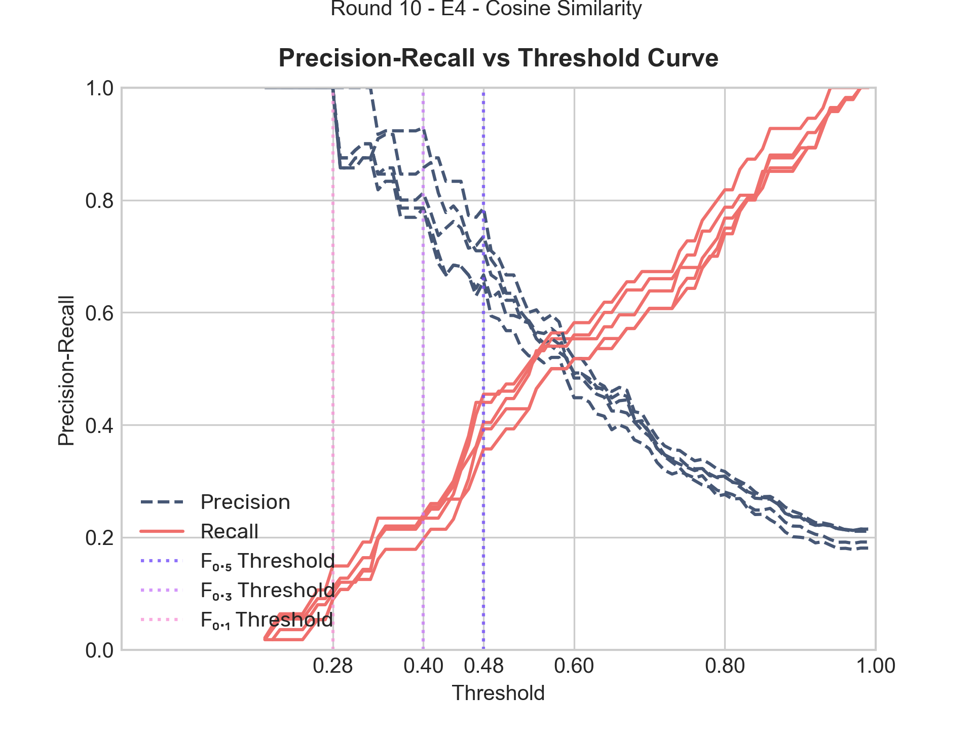
Figure 1: Precisions and recalls of all five folds in the cross-validation round 10 of model E4_COS on English data

Appendix D Cross-validation overview

$F_{0.3}$-score
	English				Swedish
	DEFAULT		SUB.		DEFAULT		SUB.
	COS	SPR	COS	SPR	COS	SPR	COS	SPR
E0	0.466	0.523	0.477	0.452	0.417	0.419	0.413	0.400
E1	0.589	0.590	0.583	0.592	0.451	0.443	0.413	0.399
E2	0.579	0.562	0.566	0.590	0.425	0.431	0.411	0.408
E3	0.494	0.523	0.493	0.489	0.428	0.431	0.397	0.392
E4	0.613	0.584	0.593	0.612
G0	0.270	0.280	0.255	0.267	0.349	0.371	0.345	0.340
G1	0.227	0.220	0.226	0.209	0.600	0.606	0.549	0.537
G2	0.260	0.223	0.264	0.245	0.550	0.612	0.564	0.547
G3	0.217	0.259	0.275	0.256	0.625	0.617	0.599	0.621

Table 6: Results of cross-validation. Performance is given as average $F_{0.3}$ across rounds and folds

Appendix E Cross-validation in round 10 of model E4_COS for English

	Average		Fold 1		Fold 2		Fold 3		Fold 4		Fold 5
	Training	Test	Training	Test	Training	Test	Training	Test	Training	Test	Training	Test
Threshold	0.396		0.340		0.350		0.480		0.410		0.400
Precision	0.842	0.720	0.846	1.000	0.833	1.000	0.735	0.500	0.867	0.600	0.929	0.500
Recall	0.272	0.215	0.234	0.105	0.179	0.400	0.455	0.182	0.260	0.188	0.232	0.200
$\mathbf{F_{0.3}}$	0.701	0.573	0.696	0.588	0.640	0.890	0.700	0.437	0.727	0.508	0.744	0.445
random_$\mathbf{F_{0.3}}$	0.335	0.331	0.328	0.336	0.328	0.400	0.358	0.000	0.328	0.528	0.334	0.392
frequency_$\mathbf{F_{0.3}}$	0.598	0.549	0.563	0.707	0.544	0.790	0.607	0.365	0.649	0.440	0.628	0.445

Table 7: Cross-validation results in round 10 of model E4_COS when maximizing $F_{0.3}$-score on English data. Column “SUB.” gives results for models where the target word was substituted with the headword

Appendix F Inter-annotator agreement

	English			Swedish
	All	Modern	Historic	All	Modern	Historic
A1 vs. A2	0.331	0.392	0.276	0.408	0.506	0.317
A1 vs. A3	0.273	0.333	0.220	0.575	0.614	0.527
A2 vs. A3	0.561	0.580	0.544	0.524	0.655	0.353
Full	0.389	0.434	0.349	0.480	0.588	0.371

Table 8: Inter-annotator agreement using Krippendorff’s alpha of annotation phase I. The labels A1–A3 represent different annotators across languages. The label “-” is excluded from the data before calculating agreement

	English			Swedish
	All	Modern	Historic	All	Modern	Historic
A1 vs. A2	0.335	0.310	0.347	0.539	0.566	0.456
A1 vs. A3	0.342	0.291	0.397	0.558	0.546	0.552
A2 vs. A3	0.464	0.490	0.374	0.608	0.641	0.526
Full	0.384	0.368	0.375	0.559	0.584	0.490

Table 9: Inter-annotator agreement using Krippendorff’s alpha of annotation phase II. The labels A1–A3 represent different annotators across languages. The label “-” is excluded from the data before calculating agreement

Appendix G Comparison of annotation results per corpus

	Phase I: Random sample			Phase II: Model prediction
Usages	All	Modern	Historical	All	Modern	Historical
total	474	232	242	322	210	112
excluded	1	1	0	0	0	0
remaining	473	231	242	322	210	112
assigned	428	208	220	277	176	101
unassigned	45 (9.5%)	23 (9.9%)	22 (9.1%)	45 (13.98%)	34 (16.2%)	11 (9.8%)

Table 10: Annotation results on English corpora

	Phase I: Random sample			Phase II: Model prediction
Usages	All	Modern	Historical	All	Modern	Historical
total	706	337	369	1001	478	523
excluded	52	4	28	74	9	65
remaining	674	333	341	927	469	458
assigned	562	293	269	327	224	103
unassigned	112 (16.6%)	40 (12.0%)	72 (21.1%)	600 (64.7%)	245 (52.2%)	355 (77.5%)

Table 11: Annotation results on Swedish corpora

References

- Adesam et al. (2019) Yvonne Adesam, Dana Dannélls, and Nina Tahmasebi. 2019. Exploring the quality of the digital historical newspaper archive kubhist. In Proceedings of the Digital Humanities in the Nordic Countries 4th Conference, Copenhagen, Denmark, March 5-8, 2019., pages 9–17.
- Alatrash et al. (2020) Reem Alatrash, Dominik Schlechtweg, Jonas Kuhn, and Sabine Schulte im Walde. 2020. CCOHA: Clean Corpus of Historical American English. In Proceedings of the 12th Language Resources and Evaluation Conference, pages 6958–6966, Marseille, France. European Language Resources Association.
- Allén (1981) Sture Allén. 1981. The lemma-lexeme model of the swedish lexical data base. In Ralph Bo, editor, Modersmålet i fäderneslandet. Ett urval uppsatser under fyrtio år av Sture Allén., pages 268–278. Meijerbergs arkiv för svensk ordforskning 25.
- Burchardt et al. (2009) Aljoscha Burchardt, Katrin Erk, Anette Frank, Andrea Kowalski, Sebastian Padó, and Manfred Pinkal. 2009. Framenet for the semantic analysis of german: Annotation, representation and automation. Multilingual FrameNets in Computational Lexicography: methods and applications, 200:209–244.
- Cassotti et al. (2023) Pierluigi Cassotti, Lucia Siciliani, Marco DeGemmis, Giovanni Semeraro, and Pierpaolo Basile. 2023. XL-LEXEME: WiC pretrained model for cross-lingual LEXical sEMantic changE. In Proceedings of the 61st Annual Meeting of the Association for Computational Linguistics (Volume 2: Short Papers), pages 1577–1585, Toronto, Canada. Association for Computational Linguistics.
- Chen et al. (2021) Howard Chen, Mengzhou Xia, and Danqi Chen. 2021. Non-parametric few-shot learning for word sense disambiguation. In Proceedings of the 2021 Conference of the North American Chapter of the Association for Computational Linguistics: Human Language Technologies, pages 1774–1781, Online. Association for Computational Linguistics.
- Davies (2012) Mark Davies. 2012. Expanding Horizons in Historical Linguistics with the 400-Million Word Corpus of Historical American English. Corpora, 7(2):121–157.
- Devlin et al. (2019) Jacob Devlin, Ming-Wei Chang, Kenton Lee, and Kristina Toutanova. 2019. BERT: Pre-training of deep bidirectional transformers for language understanding. In Proceedings of the 2019 Conference of the North American Chapter of the Association for Computational Linguistics: Human Language Technologies, Volume 1 (Long and Short Papers), pages 4171–4186, Minneapolis, Minnesota. Association for Computational Linguistics.
- Diday and Simon (1976) E. Diday and J. C. Simon. 1976. Clustering Analysis, pages 47–94. Springer Berlin Heidelberg, Berlin, Heidelberg.
- Erk (2006) Katrin Erk. 2006. Unknown word sense detection as outlier detection. In Proceedings of the Human Language Technology Conference of the NAACL, Main Conference, pages 128–135, New York City, USA. Association for Computational Linguistics.
- Erk et al. (2013) Katrin Erk, Diana McCarthy, and Nicholas Gaylord. 2013. Measuring word meaning in context. Computational Linguistics, 39(3):511–554.
- Fellbaum (2005) Christiane Fellbaum. 2005. Wordnet and wordnets. encyclopedia of language and linguistics.
- Firth (1957) John R Firth. 1957. A synopsis of linguistic theory, 1930-1955. Studies in linguistic analysis.
- Goldhahn et al. (2012) Dirk Goldhahn, Thomas Eckart, and Uwe Quasthoff. 2012. Building large monolingual dictionaries at the Leipzig corpora collection: From 100 to 200 languages. In Proceedings of the Eighth International Conference on Language Resources and Evaluation (LREC’12), pages 759–765, Istanbul, Turkey. European Language Resources Association (ELRA).
- Harris (1954) Zellig S. Harris. 1954. Distributional structure. Word, 10:146–162.
- Hu et al. (2019) Renfen Hu, Shen Li, and Shichen Liang. 2019. Diachronic sense modeling with deep contextualized word embeddings: An ecological view. In Proceedings of the 57th Annual Meeting of the Association for Computational Linguistics, pages 3899–3908, Florence, Italy. Association for Computational Linguistics.
- Jana et al. (2020) Abhik Jana, Animesh Mukherjee, and Pawan Goyal. 2020. Network measures: A new paradigm towards reliable novel word sense detection. Information Processing & Management, 57(6).
- Krippendorff (2018) Klaus Krippendorff. 2018. Content Analysis: An Introduction to Its Methodology. SAGE Publications.
- Kumar et al. (2019) Sawan Kumar, Sharmistha Jat, Karan Saxena, and Partha Talukdar. 2019. Zero-shot word sense disambiguation using sense definition embeddings. In Proceedings of the 57th Annual Meeting of the Association for Computational Linguistics, pages 5670–5681, Florence, Italy. Association for Computational Linguistics.
- Kurtyigit et al. (2021) Sinan Kurtyigit, Maike Park, Dominik Schlechtweg, Jonas Kuhn, and Sabine Schulte im Walde. 2021. Lexical Semantic Change Discovery. In Proceedings of the 59th Annual Meeting of the Association for Computational Linguistics and the 11th International Joint Conference on Natural Language Processing (Volume 1: Long Papers), Online. Association for Computational Linguistics.
- Kågebäck and Salomonsson (2016) Mikael Kågebäck and Hans Salomonsson. 2016. Word sense disambiguation using a bidirectional lstm.
- Laicher et al. (2021) Severin Laicher, Sinan Kurtyigit, Dominik Schlechtweg, Jonas Kuhn, and Sabine Schulte im Walde. 2021. Explaining and Improving BERT Performance on Lexical Semantic Change Detection. In Proceedings of the 16th Conference of the European Chapter of the Association for Computational Linguistics: Student Research Workshop, pages 192–202, Online. Association for Computational Linguistics.
- Lau et al. (2014) Jey Han Lau, Paul Cook, Diana McCarthy, Spandana Gella, and Timothy Baldwin. 2014. Learning word sense distributions, detecting unattested senses and identifying novel senses using topic models. In Proceedings of the 52nd Annual Meeting of the Association for Computational Linguistics (Volume 1: Long Papers), pages 259–270, Baltimore, Maryland. Association for Computational Linguistics.
- Lau et al. (2012) Jey Han Lau, Paul Cook, Diana McCarthy, David Newman, and Timothy Baldwin. 2012. Word sense induction for novel sense detection. In Proceedings of the 13th Conference of the European Chapter of the Association for Computational Linguistics, pages 591–601, Stroudsburg, PA, USA.
- Lautenschlager (2023) Jonathan Lautenschlager. 2023. Detection of non-recorded word senses. Bachelor thesis, University of Stuttgart.
- Lesk (1986) Michael Lesk. 1986. Automatic sense disambiguation using machine readable dictionaries: How to tell a pine cone from an ice cream cone. In Proceedings of the 5th Annual International Conference on Systems Documentation, SIGDOC ’86, page 24–26, New York, NY, USA. Association for Computing Machinery.
- Martinc et al. (2020) Matej Martinc, Syrielle Montariol, Elaine Zosa, and Lidia Pivovarova. 2020. Capturing evolution in word usage: Just add more clusters? In Companion Proceedings of the Web Conference 2020, WWW ’20, pages 343––349, New York, NY, USA. Association for Computing Machinery.
- Miller (1994) George A. Miller. 1994. WordNet: A lexical database for English. In Human Language Technology: Proceedings of a Workshop held at Plainsboro, New Jersey, March 8-11, 1994.
- Navigli (2009) Roberto Navigli. 2009. Word sense disambiguation: A survey. ACM Comput. Surv., 41(2).
- Peters et al. (2018a) Matthew Peters, Mark Neumann, Mohit Iyyer, Matt Gardner, Christopher Clark, Kenton Lee, and Luke Zettlemoyer. 2018a. Deep contextualized word representations. In Proceedings of the 2018 Conference of the North American Chapter of the Association for Computational Linguistics: Human Language Technologies, pages 2227–2237, New Orleans, LA, USA.
- Peters et al. (2018b) Matthew E. Peters, Mark Neumann, Mohit Iyyer, Matt Gardner, Christopher Clark, Kenton Lee, and Luke Zettlemoyer. 2018b. Deep contextualized word representations.
- Pilehvar and Camacho-Collados (2019) Mohammad Taher Pilehvar and Jose Camacho-Collados. 2019. WiC: the word-in-context dataset for evaluating context-sensitive meaning representations. In Proceedings of the 2019 Conference of the North American Chapter of the Association for Computational Linguistics: Human Language Technologies, Volume 1 (Long and Short Papers), pages 1267–1273, Minneapolis, Minnesota. Association for Computational Linguistics.
- Rachinskiy and Arefyev (2022) Maxim Rachinskiy and Nikolay Arefyev. 2022. GlossReader at LSCDiscovery: Train to select a proper gloss in english – discover lexical semantic change in spanish. In Proceedings of the 3rd International Workshop on Computational Approaches to Historical Language Change, Dublin, Ireland. Association for Computational Linguistics.
- Reimers and Gurevych (2019) Nils Reimers and Iryna Gurevych. 2019. Sentence-bert: Sentence embeddings using siamese bert-networks.
- Salton and McGill (1983) Gerard Salton and Michael J McGill. 1983. Introduction to Modern Information Retrieval. McGraw - Hill Book Company, New York.
- Scarlini et al. (2020) Bianca Scarlini, Tommaso Pasini, and Roberto Navigli. 2020. Sensembert: Context-enhanced sense embeddings for multilingual word sense disambiguation. Proceedings of the AAAI Conference on Artificial Intelligence, 34(05):8758–8765.
- Schlechtweg et al. (2020) Dominik Schlechtweg, Barbara McGillivray, Simon Hengchen, Haim Dubossarsky, and Nina Tahmasebi. 2020. SemEval-2020 Task 1: Unsupervised Lexical Semantic Change Detection. In Proceedings of the 14th International Workshop on Semantic Evaluation, Barcelona, Spain. Association for Computational Linguistics.
- Schütze (1998) Hinrich Schütze. 1998. Automatic word sense discrimination. Computational linguistics, 24(1):97–123.
- Spearman (1904) Charles Spearman. 1904. The proof and measurement of association between two things. American Journal of Psychology, 15:88–103.
- Språkbanken (downloaded in 2019) Språkbanken. downloaded in 2019. The Kubhist Corpus, v2. Department of Swedish, University of Gothenburg.
- Tabasi et al. (2022) Mohsen Tabasi, Kiamehr Rezaee, and Mohammad Taher Pilehvar. 2022. Exploiting language model prompts using similarity measures: A case study on the word-in-context task. In Proceedings of the 60th Annual Meeting of the Association for Computational Linguistics (Volume 2: Short Papers), pages 325–332, Dublin, Ireland. Association for Computational Linguistics.
- Vaswani et al. (2017) Ashish Vaswani, Noam Shazeer, Niki Parmar, Jakob Uszkoreit, Llion Jones, Aidan N. Gomez, Lukasz Kaiser, and Illia Polosukhin. 2017. Attention is all you need.
- Weaver (1949/1955) Warren Weaver. 1949/1955. Translation. In William N. Locke and A. Donald Boothe, editors, Machine Translation of Languages, pages 15–23. MIT Press, Cambridge, MA. Reprinted from a memorandum written by Weaver in 1949.