Conformally related vacuum gravitational waves and their symmetries

Abstract

A special conformal transformation which carries a vacuum gravitational wave into another vacuum one is built by using Möbius-redefined time. It can either transform a globally defined vacuum wave into a vacuum sandwich wave, or carry the gravitational wave into itself. The first type, illustrated by linearly and circularly polarized vacuum plane gravitational waves, permutes the symmetries and the geodesics. Our pp waves with conformal ${\rm O}(2,1)$ symmetry of the second type, which seem to have escaped attention so far, are anisotropic generalizations of the familiar inverse-square profile. An example inspired by molecular physics, for which the particle can escape, or perform periodic motion, or fall into the singularity is studied in detail.

I Introduction

We consider special class of gravitational wave (GW) space-times whose metric is written in Brinkmann coordinates Brinkmann as,

$$ds^{2}=dX^{2}+dY^{2}+2dUdV-2H(U,\mathbf{X})\,dU^{2}\,.$$ (I.1)

Here $U$ and $V$ are light-cone coordinates, $X$ and $Y$ represent the transverse plane and $H(U,\mathbf{X})$ is the wave profile. Brinkmann space-times are smooth Lorentz manifolds endowed with a covariantly constant null Killing vector field $\xi=\partial_{V}$ DGH91 . Such structures arised before in the study of the one-parameter central extension of the Galilei group Barg54 called the Bargmann group DBKP . In the proposed Kaluza-Klein-type “Bargmann” framework DBKP ; DGH91 ; Eisenhart ; Burdet1985 the motions in ordinary space are obtained by projecting out the “vertical” null direction along the coordinate $V$ and identifying the other null coordinate, $U$, with Newtonian time. The profile $H(U,\mathbf{X})$ is the Newtonian potential Eisenhart ; Burdet1985 ; DGH91 .

An insight is provided by the so-called memory effect ZelPol ; Braginsky1985 ; Grishchuk1989 ; Ehlers ; Sou73 which amounts to studying test particles initially at rest by using the symmetries of the corresponding background space-time. It is particularly convenient to use conformal symmetries Carroll4GW ; Zhang:2017rno ; Zhang:2017geq ; Zhang:2018srn ; Marsot:2021tvq ; EZHrev generated by conformal Killing vectors (CKV) ,

$$\mathcal{L}_{W}g_{ab}=2\psi g_{ab}\,,$$ (I.2)

where $\psi$ is a smooth function of the coordinates Bondi:1958aj ; Sippel1986 ; exactsol ; MaMa ; Keane:2004dpc . In flat Minkowski space-time, the conformal Lie algebra of CKVs is $15$ dimensional. The same number of dimensions arises for conformally flat space-times, which include, in addition to Minkowski space-time, also that for oscillator and for a linear potential Niederer1973 ; Burdet1985 ; Silagadze2021 ; ZZH2022 ; DGH91 ; Penrose2022 ; Dunajski23 ; Sen:2022vig  .

The maximal number of symmetries of a non-conformally-flat space-time is $7$ Keane:2004dpc ; MaMa ; exactsol . Their research is simplified when the space-time is conformally related to one whose symmetries are known, and therefore the CKVs are interchanged. This happens, in particular, for the time redefinition (II.1) below, proposed in Keane:2004dpc ; Gibbons2014 .

In this paper we study a special time-redefined conformal transformation which (i) either interchanges two vacuum GWs (as illustrated by linearly polarized plane GWs (LPP) and circularly polarized vacuum plane GWs (CPP) Zhang2022 ; Elbistan:2022umq ; Masterov , or (ii) leaves the wave form-invariant (Secs. III and IV) as illustrated by a special gravitational wave inspired by the anisotropic ${\rm O}(2,1)$ invariant field of a polar molecule Camblong:2001zt ; Camblong:2003mz ; Moroz:2009nm .

II Conformal transformations of gravitational waves

The GW space-time, $ds^{2}$ in (I.1), can be transformed into another GW, $d\widetilde{s}^{2}$, by a special conformal transformation with redefined time $f(\widetilde{U})$ Gibbons2014 ; Keane:2004dpc  ,

$$U=f(\tilde{U}),\qquad\mathbf{X}=\sqrt{\stackrel{{\scriptstyle{\raise 0.5pt\hbox{$\scriptstyle\circ$}}}}{{f}}}\,\mathbf{\widetilde{X}},\qquad V=\tilde{V}-\frac{1}{4}\frac{\stackrel{{\scriptstyle{\raise 0.5pt\hbox{$\scriptstyle\circ$}}{\raise 0.5pt\hbox{$\scriptstyle\circ$}}}}{{f}}}{\stackrel{{\scriptstyle{\raise 0.5pt\hbox{$\scriptstyle\circ$}}}}{{f}}}\,\mathbf{\widetilde{X}}^{2}\,,$$ (II.1)

where $(\stackrel{{\scriptstyle{\raise 0.5pt\hbox{$\scriptstyle\circ$}}}}{{\cdot}})$ means $d/d\widetilde{U}$. The corresponding conformal relation is,

$$ds^{2}=\Omega^{2}d\widetilde{s}^{2}=\stackrel{{\scriptstyle{\raise 0.5pt\hbox{$\scriptstyle\circ$}}}}{{f}}d\widetilde{s}^{2}\,,$$ (II.2)

$$d\widetilde{s}^{2}=d\widetilde{\mathbf{X}}^{2}+2d\widetilde{U}d\widetilde{V}-2\widetilde{H}(\widetilde{U},\widetilde{\mathbf{X}})d\widetilde{U}^{2}\,,$$ (II.3)

$$\mathrm{\small with}\quad\widetilde{H}(\widetilde{U},\widetilde{\mathbf{X}})=\stackrel{{\scriptstyle{\raise 0.5pt\hbox{$\scriptstyle\circ$}}}}{{f}}H\Big{[}\widetilde{\mathbf{X}}\sqrt{\stackrel{{\scriptstyle{\raise 0.5pt\hbox{$\scriptstyle\circ$}}}}{{f}}},f(\widetilde{U})\Big{]}+\frac{1}{4}\mathcal{S}_{\widetilde{U}}(f)\widetilde{\mathbf{X}}^{2},$$ (II.4)

where $\mathcal{S}_{\widetilde{U}}(f)$ is the Schwarzian derivative,

$$\mathcal{S}_{\widetilde{U}}(f)=\frac{\stackrel{{\scriptstyle\,{\raise 0.5pt\hbox{$\scriptstyle\circ$}}{\raise 0.5pt\hbox{$\scriptstyle\circ$}}{\raise 0.5pt\hbox{$\scriptstyle\circ$}}}}{{t}}\,}{\stackrel{{\scriptstyle{\raise 0.5pt\hbox{$\scriptstyle\circ$}}}}{{t}}}-\frac{3}{2}\left(\frac{\stackrel{{\scriptstyle{\raise 0.5pt\hbox{$\scriptstyle\circ$}}{\raise 0.5pt\hbox{$\scriptstyle\circ$}}}}{{t}}}{\stackrel{{\scriptstyle{\raise 0.5pt\hbox{$\scriptstyle\circ$}}}}{{t}}}\right)^{2}\,.$$ (II.5)

The vacuum condition for a pp-wave space-time (I.1) requires the Ricci tensor to vanish, $R_{\mu\nu}=0$, which implies that

$$\Delta{H}=H_{,XX}+H_{,YY}=0\,.$$ (II.6)

This condition involves only the spatial behavior of the wave profile.

The conformally related wave profile $\widetilde{H}$ in (II.4) satisfies the vacuum condition (II.6) if the Schwarzian derivative term vanishes Masterov ; ZZH2022 which implies in turn Möbius-redefined time Achour:2021lqq ,

$$U=f(\widetilde{U})=\frac{A\widetilde{U}+B}{C\widetilde{U}+D}\,,$$ (II.7)

completed into a special Möbius conformal transformation (SMCT),

$$V=\widetilde{V}+\frac{1}{2}\frac{C}{C\widetilde{U}+D}\widetilde{\mathbf{X}}^{2},\quad\mathbf{X}=\Omega\,\widetilde{\mathbf{X}}\,,\,\;\;{\quad\text{\small where}\quad}\;\Omega=\frac{\sqrt{AD-BC}}{C\widetilde{U}+D}\,.$$ (II.8)

$A$, $B$, $C$ and $D$ here are arbitrary constants such that $AD-BC\neq 0$. Under such a redefinition the metric (II.3) becomes,

$$ds^{2}\,=\,\Omega^{2}\,d\widetilde{s}^{2}\,=\,d\widetilde{\mathbf{X}}^{2}+2d\widetilde{U}d\widetilde{V}-2\Omega^{2}{H}\left(f(\widetilde{U})\,,\Omega\,\widetilde{\mathbf{X}}\right)d\widetilde{U}^{2}\,.$$ (II.9)

The new wave profile (II.9) is in general different from the initial one in (I.1) and approximates realistic situations: the particle is transformed into one which moves in a sandwich wave with a short wave zone $[U_{i},U_{j}]$ outside of which the space-times is flat Hawking ; BoPi89 ; Zhang:2017rno ; Zhang:2017geq ; Steinbauer1997 ; Podolsky:1998in ; PodSB ; Zhang:2017jma ; SBComment , further studied in Secs. III and IV.

III Conformally related vacuum gravitational waves

In this section, we focus our attention at vacuum plane GWs with line element

$$ds^{2}=dX^{2}+dY^{2}+2dUdV-\Big{[}\alpha(U)(X^{2}-Y^{2})+2\gamma(U)XY\Big{]}\,dU^{2},$$ (III.1)

where the arbitrary functions $\alpha(U)$ and $\gamma(U)$ correspond to the “$+$” and “$\times$” polarization modes. These waves are taken conformally into an approximate sandwich form (II.9) by (II.7)-(II.8) Zhang:2017rno ; Zhang:2017geq ; Podolsky:1998in ; Zhang:2017jma ; Andrzejewski:2018pwq with profile function

$$-2H=\Omega^{4}\left[\widetilde{\alpha}(\widetilde{U})(\widetilde{X}^{2}-\widetilde{Y}^{2})+2\widetilde{\gamma}(\widetilde{U})\widetilde{X}\widetilde{Y}\right].$$ (III.2)

where $\widetilde{\alpha}(\widetilde{U})=\alpha[f(\widetilde{U})]$ and $\widetilde{\gamma}(\widetilde{U})=\gamma[f(\widetilde{U})]$. The new GWs include two classes which correspond to different choices of the coefficients $A$, $B$, $C$ and $D$. $C=0$ means a dilation and a $U$-translation of the original GWs which does not bring any new insight and will therefore not considered in what follows. $C\neq 0$ introduces in turn a new, rationally-redefined scale factor. In terms of the redefined parameters $\rho=C/\sqrt{AD-BC}$ and $\delta=D/C$ which determine the width and the center of the new GW shown in FIG. 1, the conformal factor can be presented as

$$\Omega^{4}=\frac{1}{\left[\rho(U+\delta)\right]^{4}}\,.$$ (III.3)

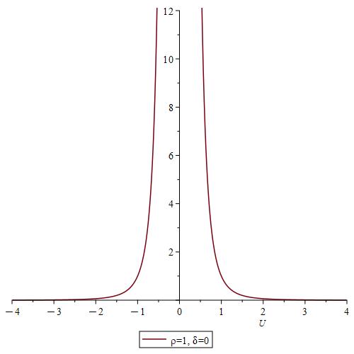
(a)

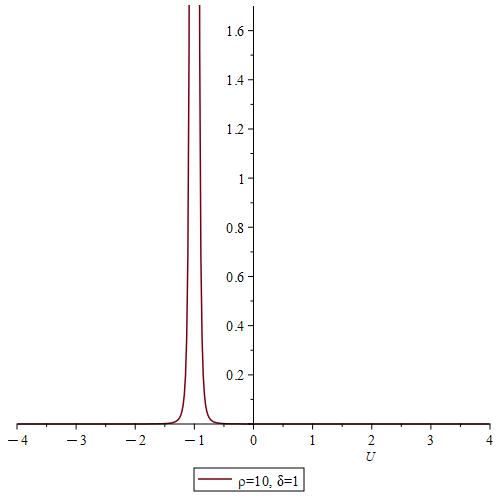
(b)

Figure 1: The conformal factor (III.4) determines the width and position of the wave (III.5): 1(a) is for parameters $\rho=1$ and $\delta=0$ and FIG. 1(b) is for $\rho=10$ and $\delta=1$, respectively.

Apart of focusing and shifting, the parameters $\rho$ and $\delta$ do not change the trajectory. Choosing $\rho=1$ and $\delta=0$ for the sake of simplicity,

$$\Omega^{4}(U)=\frac{1}{U^{4}}\,$$ (III.4)

generates the special rational transformation Keane:2004dpc ; Andrzejewski:2018zby ,

$$U=-\frac{1}{\widetilde{U}}\,,\quad\mathbf{X}=\frac{\widetilde{\mathbf{X}}}{\widetilde{U}}\,,\quad V=\widetilde{V}+\frac{\widetilde{\mathbf{X}}^{2}}{2\widetilde{U}}\,.$$ (III.5)

Eqns (2.10) and Eq. (2.11) of Andrzejewski and al. Andrzejewski:2018pwq ; Andrzejewski:2018zby are also similar, except for that their profiles tend, unlike ours, to a Dirac delta. The Möbius mapping SMCT (II.7)-(II.8) shown in FIG.1 shrinks a globally defined GW into one concentrated around a single point which then behaves as an approximate sandwich wave Zhang:2017rno ; Zhang:2017geq ; Podolsky:1998in ; Zhang:2017jma ; Andrzejewski:2018pwq .

Eqn. (III.5) is in fact the oscillator counterpart of the conformal transformation applied to planetary motion with a time-dependent gravitational constant, proposed by Dirac Dirac38 ; DGH91 .

Keane and Tupper Keane:2004dpc noted in particular that (III.5) allows us to obtain a conformally related “dual” space-time. Our Möbius-redefined time and SMCT (II.7)-(II.8) have this property also, since the inverse transformation is identical to the original one.

The general vacuum GWs in (III.1) admit Killing vectors of the form

$$\widehat{\beta}=\bm{\beta}\partial_{\bm{X}}-\dot{\beta}_{i}X^{i}\partial_{V},$$ (III.6)

where the two-vector $\bm{\beta}=(\beta_{i})$ satisfies the vectorial Sturm-Liouville equation Torre ; SL-C :

$$\ddot{\beta}_{i}(U)=K_{ij}\beta_{j}(U),\quad\mathrm{with}\quad K_{ij}=\left(\begin{array}[]{cc}\alpha(U)&\gamma(U)\\ \gamma(U)&-\alpha(U)\end{array}\right)\,$$ (III.9)

Here $\dot{(\cdot)}$ means $d/dU$.

The remarkable fact is that equation is indeed identical to the equations of motion satisfied by the transverse coordinates ${\mathbf{X}}(U)$ Lukash . Thus once we know the specific form of the Killing vector (III.6), we obtain an analytical geodesic and vice versa.

The transformation (II.7)-(II.8), carries the Killing vector (III.6) into :

$$\widehat{\widetilde{\beta}}=\widetilde{\bm{g}}(\widetilde{U}){\partial}_{\widetilde{\mathbf{X}}}-\widetilde{\mathbf{X}}\cdot\stackrel{{\scriptstyle{\raise 0.5pt\hbox{$\scriptstyle\circ$}}}}{{\widetilde{\bm{g}}}}{\partial}_{\widetilde{V}}\,,$$ (III.10)

where

$$\widetilde{\bm{g}}(\widetilde{U})=\Omega^{-1}\bm{g}\left(f(\widetilde{U})\right)$$ (III.11)

satisfies the transverse equations of motion for the conformally related GW (III.2),

$$\stackrel{{\scriptstyle{\raise 0.5pt\hbox{$\scriptstyle\circ$}}{\raise 0.5pt\hbox{$\scriptstyle\circ$}}}}{{\widetilde{{g}}}}_{j}+\widetilde{K}_{ij}\widetilde{{g}}^{i},\quad\mathrm{with}\quad\widetilde{K}_{ij}=\Omega^{4}\left(\begin{array}[]{cc}\widetilde{\alpha}(\widetilde{U})&\widetilde{\gamma}(\widetilde{U})\\ \widetilde{\gamma}(\widetilde{U})&-\widetilde{\alpha}(\widetilde{U})\end{array}\right).$$ (III.14)

Below we illustrate our point by two vacuum GWs, one linearly polarized, and the other circularly polarized. Both are globally defined and have a 7-dimensional symmetry algebra. Then we study how their symmetries and geodesics change under the transformation (III.5).

III.1 Conformally related linearly polarized vacuum GWs

1. The simplest globally defined linearly polarized vacuum GW (LPP) of Brdicka Brdicka , whose metric is,

   $$d{s}^{2}=d{X}^{2}+d{Y}^{2}+2d{U}d{V}-({X}^{2}-{Y}^{2})\,d{U}^{2}\,.$$ (III.15)

   Its CKV are obtained by solving the conformal Killing equations,

   $$W_{L}=\eta\partial_{U}+\left(2\rho V+\epsilon-\bm{X}\cdot\frac{d\bm{g}_{L}}{dU}\right)\partial_{V}+(\rho\bm{X}+\bm{g}_{L})\cdot\partial_{\bm{X}}\,,$$ (III.16)

   where

   $$\mathbf{g}_{L}(U) = (\delta_{1}\sin U+\beta_{1}\cos U)\mathbf{e}_{X}+(\delta_{2}\cosh U-\beta_{2}\sinh U)\mathbf{e}_{Y}\,.$$ (III.17)

   Here $\eta$, $\epsilon$, $\rho$, $\delta_{i}$ and $\beta_{i}$ are arbitrary constants which generate time-translations, $\widehat{E}$, vertical-translations, $\widehat{N}$, dilations, $\widehat{D}$, space-translations, $\widehat{P}_{i}$, and boosts $\widehat{G}_{i}$, respectively. These symmetries span the 7-dimensional homothetic algebra $\mathcal{E}_{7}$,

   $$[\widehat{P}_{i},\widehat{P}_{j}]=0,\quad[\widehat{G}_{i},\widehat{G}_{j}]=0,\quad[\widehat{P}_{i},\widehat{G}_{j}]=\delta_{ij}\bar{\omega}\widehat{N},\quad[\widehat{D},\widehat{N}]=-2\widehat{N},$$

   $$[\widehat{D},\widehat{G}_{i}]=-\widehat{G}_{i},\quad[\widehat{D},\widehat{P}_{j}]=-\widehat{P}_{j},\quad[\widehat{D},\widehat{E}]=0,\quad[\widehat{E},\widehat{G}_{i}]=-\widehat{P}_{i},$$

   $$[\widehat{E},\widehat{P}_{1}]=\widehat{G}_{1},\quad[\widehat{E},\widehat{P}_{2}]=-\widehat{G}_{2}\,.$$ (III.18)

   We note that the $\bm{g}_{L}$-terms in (III.16) can be collected into

   $$\bm{g}_{L}\cdot\partial_{\bm{X}}-\dot{\bm{g}_{L}}\bm{X}\cdot\partial_{V}\,.$$ (III.19)

   which is (III.6). Thus (III.17) yield also analytical solutions for the corresponding geodesics.

2. The conformal transformation (III.5) carries the Brdicka wave (III.15) into a rational LPP with damped profile,

   $$d\widetilde{s}^{2}=d\widetilde{X}^{2}+d\widetilde{Y}^{2}+2d\widetilde{U}d\widetilde{V}-\frac{1}{\widetilde{U}^{4}}(\widetilde{X}^{2}-\widetilde{Y}^{2})d\widetilde{U}^{2}.$$ (III.20)

   whose CKVs can be obtained either directly or by the conformal transformation (III.5),

   $$\widetilde{W}_{L}=\eta\widetilde{U}^{2}\partial_{\widetilde{U}}+\left(2\rho\widetilde{V}+\epsilon-\eta\frac{1}{2}\widetilde{\bm{X}}^{2}-\widetilde{\bm{X}}\cdot\stackrel{{\scriptstyle{\raise 0.5pt\hbox{$\scriptstyle\circ$}}}}{{\widetilde{\bm{g}}}}_{L}\right)\partial_{\widetilde{V}}+\left(\rho\widetilde{\bm{X}}+\eta\widetilde{U}\widetilde{\bm{X}}+\widetilde{\bm{g}}_{L}\right)\cdot\partial_{\widetilde{\bm{X}}}\,,\qquad\qquad$$ (III.21)

   where

   $$\widetilde{\mathbf{g}}_{L}(\widetilde{U})=\widetilde{U}\left(-\delta_{1}\sin\frac{1}{\widetilde{U}}+\beta_{1}\cos\frac{1}{\widetilde{U}}\right)\mathbf{e}_{X}+\widetilde{U}\left(\delta_{2}\cosh\frac{1}{\widetilde{U}}+\beta_{2}\sinh\frac{1}{\widetilde{U}}\right)\mathbf{e}_{Y}\,.\quad$$ (III.22)

   Note that the $\bm{\widetilde{g}}_{L}$-terms in (III.21) fit also into (III.10), therefore (III.22) is an analytically-found geodesics in the rational LPP GW space-time.

   The parameters represent the same symmetries as in the Brdicka case, except for $\eta$ which becomes a special Killing vector (SCKV) identified as an expansion $\widehat{K}$,

   $$\widehat{K}=U^{2}{\partial}_{U}-\frac{1}{2}\mathbf{X}^{2}{\partial}_{V}+U\mathbf{X}\cdot{\partial}_{\mathbf{X}}\,,$$ (III.23)

   which acts as a redefined-time translation $\widehat{E}={\partial}_{U}$. The commutation relations are,

   $$[\widehat{P}_{i},\widehat{P}_{j}]=0,\quad[\widehat{G}_{i},\widehat{G}_{j}]=0,\quad[\widehat{P}_{i},\widehat{G}_{j}]=\delta_{ij}\bar{\omega}\widehat{N},\quad[\widehat{D},\widehat{N}]=-2\widehat{N}\,,$$

   $$[\widehat{D},\widehat{G}_{i}]=-\widehat{G}_{i},\quad[\widehat{D},\widehat{P}_{j}]=-\widehat{P}_{j},\quad[\widehat{D},\widehat{K}]=0,\quad[\widehat{K},\widehat{G}_{i}]=-\widehat{P}_{i}\,,$$

   $$[\widehat{K},\widehat{P}_{1}]=\widehat{G}_{1},\quad[\widehat{K},\widehat{P}_{2}]=-\widehat{G}_{2}\,.$$ (III.24)

   Thus the algebra $\mathcal{E}_{7}\supset\mathcal{G}_{6}$ for the Brdicka GW (III.15) is transformed, for the rational-time LPP GW (III.20), into

   $$\mathcal{S}_{7}\supset\mathcal{E}_{6}\supset\mathcal{G}_{5}\,.$$ (III.25)

   Here $\mathcal{S}$, $\mathcal{E}$, $\mathcal{G}$ are the special conformal algebra, homothetic algebra and isometric algebra generators, respectively. The subscripts indicate the dimension of the algebra. The commutation relations do not change even if the CKV do Elbistan:2020ffe ; Keane:2004dpc .

3. The circularly polarized (CPP) GW has line element

   $$ds^{2}=dX^{2}+dY^{2}+2dUdV-\Big{[}\cos(2\omega U)(X^{2}-Y^{2})+2\sin(2\omega U)XY\Big{]}dU^{2},\qquad\quad$$ (III.26)

   where $\omega$ is an arbitrary constant frequency. The corresponding CKVs were studied, e.g., in Zhang:2018srn ; Elbistan:2022umq  :

   $$W_{C}=\eta\left[\partial_{U}+\omega\left(X{\partial}_{Y}-Y{\partial}_{X}\right)\right]+\left(2\rho V+\epsilon-\bm{X}\cdot\dot{\bm{g}}_{C}\right)\partial_{V}+(\rho\bm{X}+\bm{g}_{C})\cdot\partial_{\bm{X}}\,,\qquad$$ (III.27)

   where

   $$\mathbf{g}_{C}(U)=g_{C1}(U)\,\mathbf{e}_{X}+g_{C2}(U)\,\mathbf{e}_{Y},$$ (III.28)

   $$g_{C1}(U)=\beta_{2}\mathcal{D}_{U}\left(\sin{\omega}U\cdot\sin\omega_{-}U\right)+\delta_{2}\mathcal{D}_{U}\left(\sin{\omega}U\cdot\cos\omega_{-}U\right)$$

   $$\qquad+\beta_{1}\mathcal{D}_{U}\left(\cos{\omega}U\cdot\sin\omega_{+}U\right)-\delta_{1}\mathcal{D}_{U}\left(\cos{\omega}U\cdot\cos\omega_{+}U\right),$$ (III.29)

   $$g_{C2}(U)=-\beta_{2}\mathcal{D}_{U}\left(\cos{\omega}U\cdot\sin\omega_{-}U\right)-\delta_{2}\mathcal{D}_{U}\left(\cos{\omega}U\cdot\cos\omega_{-}U\right)$$

   $$\qquad+\delta_{1}\mathcal{D}_{U}\left(\sin{\omega}U\cdot\cos\omega_{+}U\right)-\beta_{1}\mathcal{D}_{U}\left(\sin{\omega}U\cdot\sin\omega_{+}U\right)$$ (III.30)

   represent also the analytic geodesics in the CPP GW space-time. Here $\omega_{\pm}=\sqrt{\omega^{2}\pm 1}$ and $\mathcal{D}_{U}$ is the bilinear derivative $\mathcal{D}_{U}(f\cdot g)=g\frac{df}{dU}-f\frac{dg}{dU}$ .

   The parameters $\eta$, $\rho$, $\epsilon$, $\delta_{i}$ and $\beta_{i}$ generate “screw” symmetries $\widehat{S}$ Elbistan:2022umq , namely dilations $\widehat{D}$, vertical-translations $\widehat{N}$, space-translations $\widehat{P}_{i}$, and boosts $\widehat{G}_{i}$, respectively, span a 7-d homothetic algebra $\mathcal{E}_{7}\supset\mathcal{G}_{6}$ Zhang:2018srn .

4. Inserting (III.5) into (III.26) yields the rational CPP GW whose line element is,

   $$d\widetilde{s}^{2} = d\widetilde{X}^{2}+d\widetilde{Y}^{2}+2d\widetilde{U}d\widetilde{V}$$ (III.31)

   $$-\frac{1}{\widetilde{U}^{4}}\left[\cos\left(\frac{2\omega}{\widetilde{U}}\right)(\widetilde{X}^{2}-\widetilde{Y}^{2})+2\sin\left(\frac{2\omega}{\widetilde{U}}\right)\widetilde{X}\widetilde{Y}\right]d\widetilde{U}^{2},\qquad$$

   Its CKVs are obtained as in the rational-time LPP case,

   $$\widetilde{W}_{C}=\eta\left[\partial_{\widetilde{U}}+\widetilde{U}\widetilde{\bm{X}}\cdot{\partial}_{\widetilde{\bm{X}}}+\omega\left(\widetilde{X}{\partial}_{\widetilde{Y}}-\widetilde{Y}{\partial}_{\widetilde{X}}\right)\right]$$

   $$\qquad+\left(2\rho\widetilde{V}+\epsilon-\bm{\widetilde{X}}\cdot\stackrel{{\scriptstyle{\raise 0.5pt\hbox{$\scriptstyle\circ$}}}}{{\widetilde{\bm{g}}}}_{C}\right)\partial_{\widetilde{V}}+(\rho\bm{\widetilde{X}}+\bm{\widetilde{g}}_{C})\cdot\partial_{\bm{\widetilde{X}}}\,,$$ (III.32)

   where

   $$\widetilde{\mathbf{g}}_{C}(\widetilde{U})=\widetilde{g}_{C1}(\widetilde{U})\mathbf{e}_{\widetilde{X}}+\widetilde{g}_{C2}(\widetilde{U})\mathbf{e}_{\widetilde{Y}},$$ (III.33)

   $$\widetilde{g}_{C1}=-\beta_{2}\frac{\widetilde{U}}{\omega_{+}}\mathcal{D}_{\widetilde{U}}\left(\widetilde{U}\cos\frac{\omega_{+}}{\widetilde{U}}\cdot\widetilde{U}\cos\frac{\omega}{\widetilde{U}}\right)-\delta_{2}\frac{\widetilde{U}}{\omega_{+}}\mathcal{D}_{\widetilde{U}}\left(\widetilde{U}\sin\frac{\omega_{+}}{\widetilde{U}}\cdot\widetilde{U}\cos\frac{\omega}{\widetilde{U}}\right)$$

   $$\qquad\,+\beta_{1}\frac{\widetilde{U}}{\omega}\mathcal{D}_{\widetilde{U}}\left(\widetilde{U}\cos\frac{\omega_{-}}{\widetilde{U}}\cdot\widetilde{U}\sin\frac{\omega}{\widetilde{U}}\right)-\delta_{1}\frac{\widetilde{U}}{\omega}\mathcal{D}_{\widetilde{U}}\left(\widetilde{U}\sin\frac{\omega_{-}}{\widetilde{U}}\cdot\widetilde{U}\sin\frac{\omega}{\widetilde{U}}\right),$$ (III.34)

   $$\widetilde{g}_{C2}=-\beta_{2}\frac{\widetilde{U}}{\omega_{+}}\mathcal{D}_{\widetilde{U}}\left(\widetilde{U}\cos\frac{\omega_{+}}{\widetilde{U}}\cdot\widetilde{U}\sin\frac{\omega}{\widetilde{U}}\right)-\delta_{2}\frac{\widetilde{U}}{\omega_{+}}\mathcal{D}_{\widetilde{U}}\left(\widetilde{U}\sin\frac{\omega_{+}}{\widetilde{U}}\cdot\widetilde{U}\sin\frac{\omega}{\widetilde{U}}\right)$$

   $$\qquad+\beta_{1}\frac{\widetilde{U}}{\omega}\mathcal{D}_{\widetilde{U}}\left(\widetilde{U}\cos\frac{\omega_{-}}{\widetilde{U}}\cdot\widetilde{U}\cos\frac{\omega}{\widetilde{U}}\right)-\delta_{1}\frac{\widetilde{U}}{\omega}\mathcal{D}_{\widetilde{U}}\left(\widetilde{U}\sin\frac{\omega_{-}}{\widetilde{U}}\cdot\widetilde{U}\cos\frac{\omega}{\widetilde{U}}\right).$$ (III.35)

   are also analytical geodesics in the rational CPP GW space-time.

   Here the parameters $\rho$, $\epsilon$, $\delta_{i}$, $\beta_{i}$ represent the same symmetries as for the CPP wave, — except for $\eta$, which is a new special symmetry denoted by $\widehat{S}_{K}$,

   $$\widehat{S}_{K}=\widetilde{U}^{2}{\partial}_{\widetilde{U}}-\frac{1}{2}\widetilde{\mathbf{X}}^{2}{\partial}_{\widetilde{V}}+\widetilde{U}\widetilde{\mathbf{X}}\cdot{\partial}_{\widetilde{\mathbf{X}}}+\omega(\widetilde{X}{\partial}_{\widetilde{Y}}-\widetilde{Y}{\partial}_{\widetilde{X}})\,,$$ (III.36)

   which corresponds to Eq. # (147) of Keane and Tupper in Ref. Keane:2004dpc . Its geometric meaning is obtained by integrating the Killing vector (III.36). We just present its space part,

   $$\left\{\begin{array}[]{lll}X&=&-\frac{U}{U_{0}}\left[X_{0}\cos\left(\frac{\omega(U-U_{0})}{UU_{0}}\right)+Y_{0}\sin\left(\frac{\omega(U-U_{0})}{UU_{0}}\right)\right]\\[12.0pt] Y&=&\;\;\frac{U}{U_{0}}\left[Y_{0}\cos\left(\frac{\omega(U-U_{0})}{UU_{0}}\right)-X_{0}\sin\left(\frac{\omega(U-U_{0})}{UU_{0}}\right)\right]\end{array}\right.\,,$$ (III.37)

   where $X_{0}$, $Y_{0}$ and $U_{0}$ are initial positions. It describes a “growing screw” whose size increases linearly with $U$ while its frequency decreases as shown in FIG. 2.

   

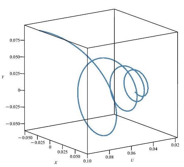
   (a)

   

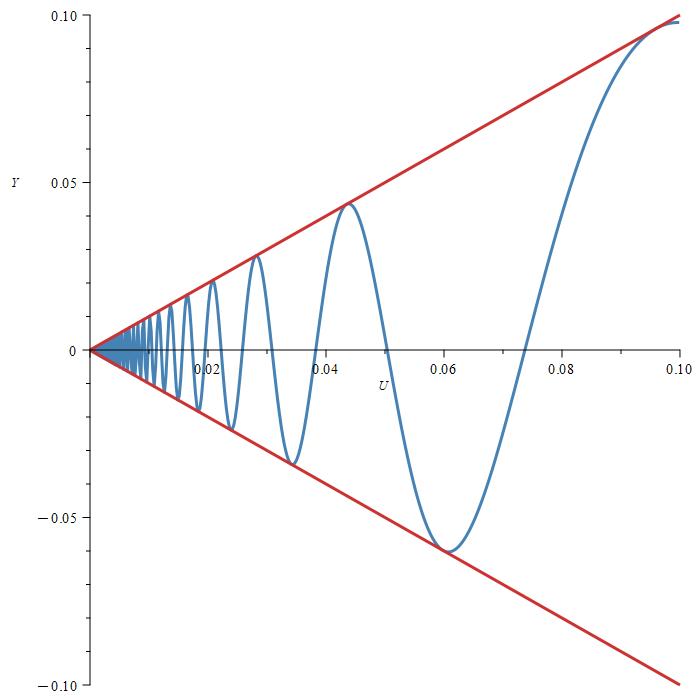
   (b)

   Figure 2: 2(a): the “screw” (III.37) of the rational CCP GW (III.31) expands linearly with $U$. FIG. 2(b) shows its projection onto the $Y-U$ plane.

   A similar “screw” has also been found for planetary motions with for time-dependent gravitational constant in Newtonian gravity Dirac38 ; DGH91 .

III.2 Gedesics, found numerically and analytically

Now we compare the how geodesics change under applying the transformation (III.5).

1. Numerical solutions are shown in FIG. 3 for the LPP GW of Brdicka, (III.15), and for the rational LPP (III.20). Analytic solutions are obtained in turn in (III.17) for the Brdicka GW, and a piecewise function for the rational LPP GW is in turn,

   

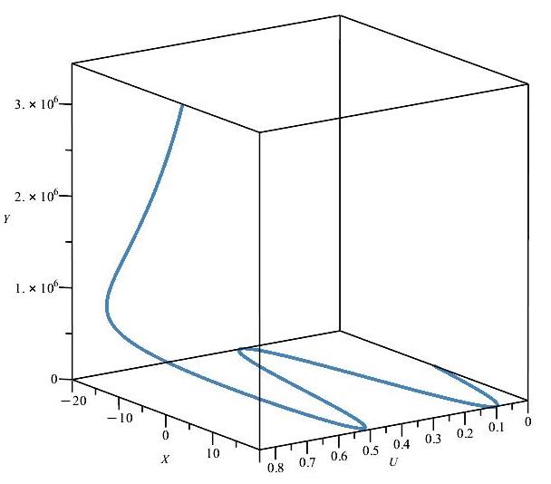
   (a)

   

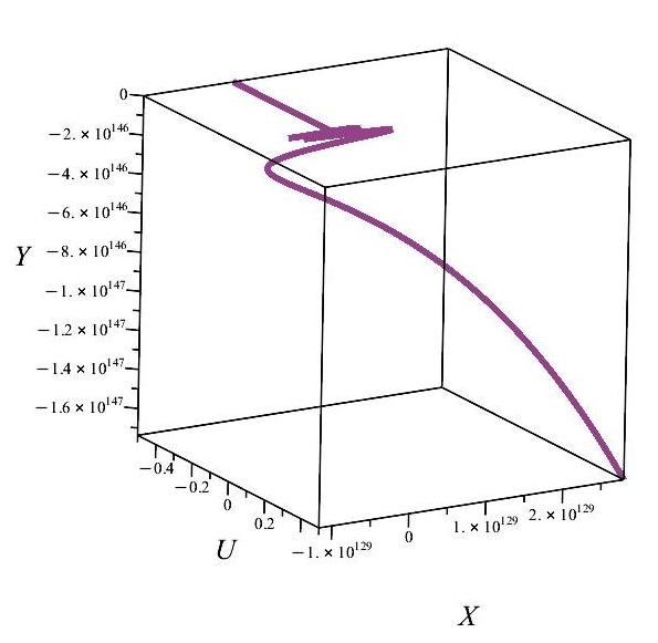
   (b)

   Figure 3: 3(a): a particle in Brdicka GW space-time (III.15) (drawn in steel blue) oscillates. It should be compared with what happens in the rational LPP GW (III.20) obtained by squeezing the wave as in (III.5) drawn in dark orchid in FIG. 3(b), for which the particle initially in rest is shaken by the GW and then escapes with approximately constant velocity due to the damping factor $U^{-1}$ after the wave has passed.

   $$\widetilde{X}(\widetilde{U})=\left\{\begin{aligned} &\widetilde{U}\sin\widetilde{U}^{-1},\qquad\qquad\qquad\qquad&\widetilde{U}<0\,,\\ &\widetilde{U}\cos\widetilde{U}^{-1},\qquad\qquad\qquad\qquad&\widetilde{U}>0\,.\end{aligned}\right.$$ (III.38)

   $$\widetilde{Y}(\widetilde{U})=\left\{\begin{aligned} &0,\quad&\widetilde{U}\leq 0\,,\\ &\widetilde{U}\left(\sinh\widetilde{U}^{-1}-\cosh\widetilde{U}^{-1}\right)\,,\quad&\widetilde{U}>0.\end{aligned}\right.$$ (III.39)

   These solutions plotted in FIG. 4 should be compared with the numerical ones in FIG.3.

   

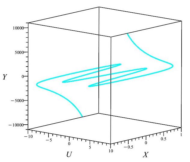
   (a)

   

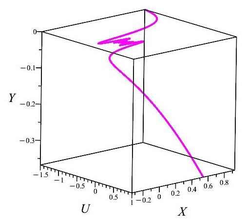
   (b)

   Figure 4: Analytically found geodesics. 4(a) shows those for the Brdicka metric (III.15), and 4(b) for the rational LPP in (III.38)-(III.39). These plots should be compared with the numerical ones in FIG. 3.

2. The geodesics of both the usual CPP GW (III.26) and the rational-time CPP GW (III.31) perform screw-like motions. FIG. 5 compares these two numerically-obtained geodesics.

   

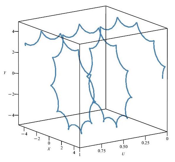
   (a)

   

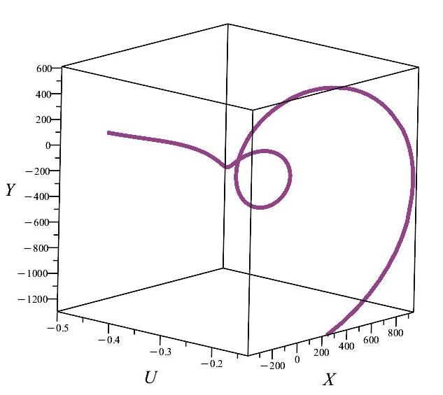
   (b)

   Figure 5: 5(a) : in the usual CPP GW (depicted in steel blue) the particle performs a “gear wheel - like” motion. 5(b) : in the rational CPP GW (in dark orchid) the particle which is at rest before the GW arrives, escapes along an expanding screw after the GW has passed. For large $U$ its velocity becomes approximately constant due to the damping factor $\widetilde{U}^{-4}$ in (III.31).

   On the other hand, (III.28) is an analytically found geodesic for the CPP GW space-time (III.26) which follows the same trajectory as 5(a) when the parameters are chosen $\omega=1.5$, $\delta_{1}=0$, $\delta_{2}=0$, $\beta_{1}=0$ and $\beta_{2}=5$.

   The rational CPP GW (III.31) admits special piecewise solutions,

   $$\widetilde{X}(\widetilde{U})=\left\{\begin{aligned} &0,\quad\widetilde{U}\leq 0,\\[4.0pt] &\frac{\widetilde{U}}{\omega}\mathcal{D}_{\widetilde{U}}\left(\widetilde{U}\cos\frac{\omega_{-}}{\widetilde{U}\;}\cdot\widetilde{U}\sin\frac{\omega}{\widetilde{U}}\right),\quad\widetilde{U}>0.\end{aligned}\right.$$ (III.40)

   $$\widetilde{Y}(\widetilde{U})=\left\{\begin{aligned} &0,\quad\widetilde{U}\leq 0,\\[4.0pt] &\frac{\widetilde{U}}{\omega}\mathcal{D}_{\widetilde{U}}\left(\widetilde{U}\cos\frac{\omega_{-}}{\widetilde{U}\;}\cdot\widetilde{U}\cos\frac{\omega}{\widetilde{U}}\right),\quad\widetilde{U}>0\,,\end{aligned}\right.$$ (III.41)

   plotted in FIG. 6 which should be compared with the numerical solution in FIG.5(b).

   

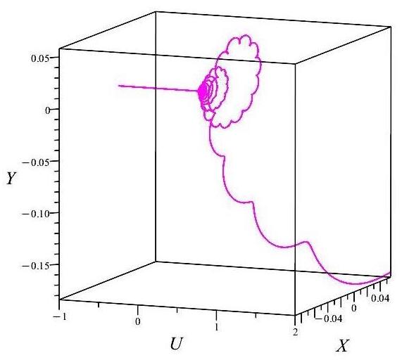
   Figure 6: The analytic rational CPP solution (III.40)-(III.41), to be compared with the numerically found one in 5(b).

   In FIG. 7 we show the variations of the velocities in FIG. 6 on $X$ and $Y$ directions.

   

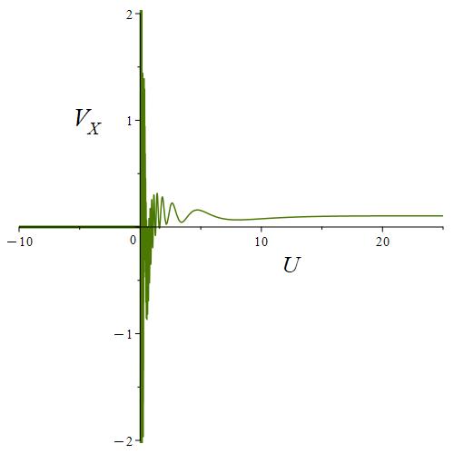
   (a)

   

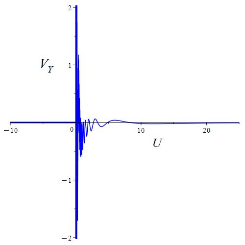
   (b)

   Figure 7: For the rational CPP GW (III.31) the velocities become approximately constant after the wave has passed due to the damping factor $\widetilde{U}^{-4}$: we get the velocity effect Grishchuk1989 ; Zhang:2018srn .

IV ${\rm O}(2,1)$-conformally invariant gravitational waves

In the previous section we discussed vacuum GWs that are carried into another vacuum GW by the special Möbius transformation (II.7)-(II.8). In this section we consider a special vacuum GWs which are invariant.

We start by completing (II.7) by the well-known $\xi$-preserving conformal transformations of the conformal Killing equations in the free Minkowski metric in $2+1$ dimensions, (I.1) with $H=0$. We get three special transformations, namely,

$$\mathrm{time}\mathrm{-}\mathrm{translation}:\ U=\widetilde{U}+\epsilon,\ \ \mathbf{X}=\widetilde{\mathbf{X}}\,,\ \ V=\widetilde{V}\,,$$ (IV.1a)

$$\mathrm{dilatation}:\ U=e^{2\delta}\widetilde{U},\ \ \mathbf{X}=e^{\delta}\widetilde{\mathbf{X}}\,,\ \ V=\widetilde{V},$$ (IV.1b)

$$\mathrm{special}\ \mathrm{conformal}\ \mathrm{transformation}:$$

$$\qquad U=\frac{\widetilde{U}}{1+\kappa\,\widetilde{U}}\,,\;\;\;\;\mathbf{X}=\frac{\widetilde{\mathbf{X}}}{1+\kappa\,\widetilde{U}}\,,\;\;\;\;V=\widetilde{V}+\frac{\kappa}{2(1+\kappa\,\widetilde{U})}\widetilde{\mathbf{X}}^{2}\,,$$ (IV.1c)

where $\epsilon$, $\delta$ and $\kappa$ are arbitrary real constants. The corresponding infinitesimal generators,

$$\mathrm{time}\mathrm{-}\mathrm{translation}:\ \widehat{E}=\partial_{U},$$ (IV.2a)

$$\mathrm{dilation}:\ \widehat{D}=U\partial_{U}+\frac{1}{2}\left(X\partial_{X}+Y\partial_{Y}\right),$$ (IV.2b)

$$\mathrm{expansion}:\ \widehat{K}=U^{2}\partial_{U}+U\big{(}X\partial_{X}+Y\partial_{Y}\big{)}-\frac{1}{2}(X^{2}+Y^{2})\partial_{V}\,,$$ (IV.2c)

span an ${\rm o}(2,1)$ algebra,

$$[\widehat{D},\widehat{E}]=-\widehat{E},\quad[\widehat{D},\widehat{K}]=\widehat{K},\quad[\widehat{E},\widehat{K}]=2\widehat{D}\,$$ (IV.3)

which generate an ${\rm O}(2,1)$ conformal group.

The ${\rm O}(2,1)$ symmetry has been considered in various physical instances:

• For a free particle SchrSymm ; DBKP ; DGH91 or in Chern-Simons field theory JackiwPiCS ; DHP1 ; DHP2 it extends the Galilei to the Schrödinger algebra SchrSymm . All Schrödinger-symmetric systems are derived, in $d\geq 3$ space dimensions, from the vanishing of the Weyl DHP2 or in in $d=1$ from that of the Cotton tensor Zurab , respectively.

• An inverse-square potential could be added DBKP ; Jacobi ; SchrSymm ; DHP2 ; DHP1 ; JackiwPiCS ; AFF ; ScalingZCEH ; Zurab . Applications include the interaction of a polar molecule with an electron Camblong:2001zt ; Moroz:2009nm (which will be discussed further in subsec.V), the Efimov effect Efimov:1973awb ; Moroz:2009nm , near-horizon fields of black holes Camblong:2003mz ; Claus ; Moroz:2009nm and the vacuum AdS/CFT correspondence Gubser:1998bc ; Moroz:2009nm ; Witten:1998qj ;

• A Dirac-monopole and a magnetic vortex Jackiw:1980mm ; Jackiw:1989qp  .

Hence we focus our attention at vacuum gravitational waves with ${\rm O}(2,1)$ symmetry. For symplicity, we focus our investigations to the planar case with coordinates $X,\,Y$. Substituting the three vectors in (IV.2a)-(IV.2c) into the conformal Killing equation (I.2) for the Brinkmann metric (I.1) leaves us with,

$$\mathrm{time}\mathrm{-}\mathrm{translation}:\ H_{,U}=0\,,$$ (IV.4a)

$$\mathrm{dilatations}:\ UH_{,U}+XH_{,X}+YH_{,Y}+2H=0\,,$$ (IV.4b)

$$\mathrm{special}\ \mathrm{conformal}\ \mathrm{transformation}:\ 2UH_{,U}+XH_{,X}+YH_{,Y}+2H=0\,.$$ (IV.4c)

Note that (IV.4b) and (IV.4c) differ only in the coefficients of their first terms – which involves the generator of time translation symmetry, (IV.4a).

Solving these equations with the vacuum condition (II.6) yields, for an exact plane wave, the line element,

$$\;\;\displaystyle{ds_{O21}^{2}=dX^{2}+dY^{2}+2dUdV-2\left(\frac{C_{1}(X^{2}-Y^{2})+2C_{2}XY}{R^{4}}\right)dU^{2}\,,}\;\;$$ (IV.5)

where $R^{2}=X^{2}+Y^{2}$; $C_{1}$ and $C_{2}$ are arbitrary constants. The proof follows at once from that dilatation symmetry (IV.4b), combined with time-translation-invariance (IV.4a) imply indeed, by Euler’s formula, that the potential is homogeneous of order $(-2)$.

The potential (IV.5) breaks the rotational symmetry, however still allows for the conformal ${\rm O}(2,1)$ symmetry of the inverse-square potential AFF ; DBKP ; DGH91 to the anisotropic case. It should be compared to the statement DHP2 ; Zurab which says that the profiles of the only Bargmann manifolds with Schrödinger symmetry correspond, in 3+1 dimensions, to an (i) isotropic oscillator, to an (ii) inverse-square potential with constant coefficient, to a (iii) uniform force field.

The special GW (IV.5) satisfies, for an arbitrary linear combination of $\widehat{E},\,\widehat{D},\,\widehat{K}$ in (IV.2a)-(IV.2c), the conformal Killing equations (I.2) with,

$$W=a\widehat{E}+b\widehat{D}+c\widehat{K}=(a+bU+cU^{2}){\partial}_{U}-c\frac{1}{2}\mathbf{X}^{2}{\partial}_{V}+(cU+\frac{b}{2})\mathbf{X}\cdot{\partial}_{\mathbf{X}}\,,$$ (IV.6)

where $a$, $b$ and $c$ are arbitrary constants. By integrating the $U$ component of (IV.6), the associated SKV reduces to the Möbius-redefined time (II.7) with $\mathbf{X},\,A$, etc replaced by, $\tilde{{\mathbf{X}}}$ and by,

$$\tilde{A}=-\left[\frac{b}{2}+\frac{\sqrt{4ac-b^{2}}}{2\tan\left(\frac{\eta\sqrt{4ac-b^{2}}}{2}\right)}\right],\;\;\tilde{B}=-c,\;\;\tilde{C}=a,\;\;\tilde{D}=-\left[\frac{\sqrt{4ac-b^{2}}}{2\tan\left(\frac{\eta\sqrt{4ac-b^{2}}}{2}\right)}\right]\,,\quad$$ (IV.7)

where $\eta$ is the parameter of the integral curve. In conclusion, the special gravitational wave (IV.5) is form-invariant under the SMCT (II.8).

The metric (IV.5) is conveniently presented in cylindrical coordinates $(R,\theta)$,

$$ds_{O21}^{2}=dR^{2}+R^{2}d\theta^{2}+2dUdV-2\left(\frac{C_{1}\cos 2\theta+C_{2}\sin 2\theta}{R^{2}}\right)dU^{2}\,,$$ (IV.8)

reminiscent of the potential for the interaction between a polar molecule and an electron Camblong:2001zt ; Camblong:2003mz ,

$$H\equiv H(r,\theta)=\frac{C\cos\theta}{r^{2}}\,,$$ (IV.9)

where the constant $C$ is proportional to the product of the electric charge and the dipole momentum, and $\theta$ is the polar angle in the $X-Y$ plane.

V A molecular physics-inspired spacetime

In this section, we study a vacuum spacetime inspired by polar molecules represented by the anisotropic inverse-square potential Camblong:2001zt ; Camblong:2003mz ,

$$H=\frac{C_{1}\cos 2\theta+C_{2}\sin 2\theta}{R^{2}}\,,$$ (V.1)

where $C_{1}$ and $C_{2}$ are real constants, cf. (IV.8). Postponing the $3$-dimensional problem to further study, we limit our attention at the plane. For simplicity, we put also the NR mass $M=1$. The conformal Killing vectors in (IV.2a)-(IV.2b)-(IV.2c) preserve the vertical vector $\xi={\partial}_{V}$ and therefore project to conformal symmetries of the underlying non-relativistic system providing us with three conserved quantities SchrSymm ; AFF ; DBKP ; Jacobi ,

$$\widehat{E}\quad\rightarrow\quad \mathcal{E}=\frac{\mathbf{P}^{2}}{2}+\frac{C_{1}\cos 2\theta+C_{2}\sin 2\theta}{R^{2}}\,,$$ (V.2a)

$$\widehat{D}\quad\rightarrow\quad \mathcal{D}=2\mathcal{E}U-\mathbf{P}\cdot\mathbf{X}\,,$$ (V.2b)

$$\widehat{K}\quad\rightarrow\quad \mathcal{K}=-\mathcal{E}U^{2}+\mathcal{D}U+\frac{1}{2}R^{2}\,.$$ (V.2c)

To explain in simple terms what happens, consider first dilations, (IV.2b), which leave the Lagrange density $L_{0}dU$ of a free NR particle invariant provided the time scales with the square of the factor as the position does SchrSymm . Then adding a potential $H$ changes the Lagrange density by $-HdU$, which is also invariant if $H$ is inverse-square in the radius AFF ; DBKP ; ScalingZCEH .

However dilations act only on the radial variable, therefore the potential (V.1) is left invariant. Then an easy calculation shows that the two other transformations in (IV.2) remain also unbroken. Remarkably, the associated “Noether" quantities were found by Jacobi Jacobi …60 years before Emmy Noether was born !

The Casimir operator of ${\rm O}(2,1)$ is,

$$\mathcal{C}^{2}=\mathcal{R}^{2}-\mathcal{G}_{-}^{2}-\mathcal{G}_{+}^{2},$$ (V.3)

where

$$\mathcal{R}=\frac{1}{2}\left(\frac{1}{\tau}\widehat{K}+\tau\widehat{E}\right),\quad\mathcal{G}_{-}=\frac{1}{2}\left(\frac{1}{\tau}\widehat{K}-\tau\widehat{E}\right),\quad\mathcal{G}_{+}=\widehat{D}\,$$ (V.4)

generate a compact $\mathrm{SO}(2)$ group of rotations, augmented with two non-compact two dimensional boosts. Here $\tau$ is a positive fixed parameter with the dimension of time. See Ref. Jackiw:1989qp for details. The Casimir operator can also be written as,

$$\mathcal{C}^{2} = {J}^{2}+2\left(C_{1}\cos 2\theta+C_{2}\sin 2\theta\right),$$ (V.5)

where ${J}=\mathbf{R}\times\mathbf{V}$ is the orbital angular momentum. ( The angular momentum in 2 dimensions is just a scalar, namely the 3rd component of the 3-dimensionalone, $J_{z}$. The conserved quantity generated by translations along the $V$ coordinate and interpreted as the mass of the underlying non-relativistic system DBKP ; Eisenhart ; DGH91 was scaled to unity).

A lightlike particle in the special GW background (IV.5) (viewed, in the Bargmann framework, as a massive non-relativistic particle in one dimension less) moves along null geodesics. In cylindrical coordinates,

$$\frac{\;d^{2}R}{dU^{2}}-R\left(\frac{d\theta}{dU}\right)^{2}-\frac{2\left[C_{1}\cos 2\theta+C_{2}\sin 2\theta\right]}{R^{3}}=0\,,$$ (V.6)

$$\frac{\;d^{2}\theta}{dU^{2}}+\frac{2}{R}\frac{dR}{dU}\frac{d\theta}{dU}-\frac{2\left[C_{1}\sin 2\theta-C_{2}\cos 2\theta\right]}{R^{4}}=0\,.$$ (V.7)

Let us assume, for simplicity, that $C_{1}=0$ so that the planar metric (IV.8) has only one polarization state,

$$\;\;\displaystyle{ds^{2}=dR^{2}+R^{2}d\theta^{2}+2dUdV-2\left(\frac{C_{2}\sin 2\theta}{R^{2}}\right)\,dU^{2}\,,}\;\;$$ (V.8)

For $C_{2}=0$ we get Minkowski-space which has no interest for us. Then $C_{2}>0$ can be achieved by shifting $\theta$. Henceforth we set $C_{2}=1$.

The metric (V.8) is the “Bargmannian” form Eisenhart ; DBKP ; DGH91 of the anisotropic version of a NR particle in an inverse-square potential

$$H(R,\theta)=\frac{\sin 2\theta}{R^{2}}\,,$$ (V.9)

shown in FIG.8. Its anisotropy is manifest by realizing that for fixed $R=R_{0}$, $H(R,\theta)$ is proportional to $\sin 2\theta$.

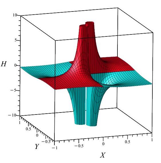
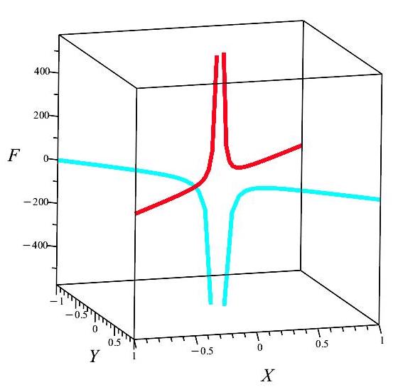
(a)                                                                      (b)

Figure 8: (a) The potential (V.8) alternates between repulsive (NE-SW) and attractive (NW-SE) forms, changing sign at every quadrant. The apparent doubling of the “chimneys and sinks” in FIG.a are computer artifacts as confirmed by FIG.b. The only singularity is at the origin.

The nature of the potential (V.8) is determined by the sign of the coefficient of $dU^{2}$ — the potential of the underlying non-relativistic dynamics DBKP ; DGH91 — which alternates at every quadrant. Its behavior is conveniently studied by plotting the force, FIG.9: It is repulsive for $0<\theta<\pi/2$ and for $\pi<\theta<3\pi/2$, and attractive for $\pi/2<\theta<\pi$ and for $3\pi/2<\theta<2\pi$. The force is maximal on the separation “crosslines” at $\theta=k\pi/2,\,k=0,1,2,3$, where the repulsive potential becomes attractive and vice versa, cf. (V.9). It is obviously symmetric w.r.t. $\theta\to\theta+\pi$.

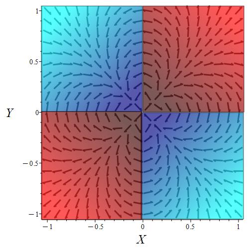
Figure 9: The force $-{{\bm{\nabla}}}{H}$ alternates at every quarter-of-circle between repulsive (NE - SW) and attractive (NW - SE) regions. The force is maximally repulsive along the “crests” at $\pi/4$ and $5\pi/4$ and maximally attractive in the “valley bottoms” at $3\pi/4$ and $7\pi/4$, respectively.

A qualitative insight into the possible motions can be obtained by using the conformal ${\rm o}(2,1)$ symmetry. For simplicity we restict our attention at what happens to a particle that we simply put at $U=U_{0}$ to some position $(R_{0},\theta_{0})$ with vanishing initial velocity. Then the conserved quantities (V.2) generated by ${\rm o}(2,1)$ reduce, putting $M=1,\,C_{1}=0,\,C_{2}=1$ for simplicity, to

$$\mathcal{E}_{0}=\frac{\sin 2\theta_{0}}{R_{0}^{2}}\,,$$ (V.10a)

$$\mathcal{D}_{0}=2\mathcal{E}_{0}U_{0}\,,$$ (V.10b)

$$\mathcal{K}_{0}=-\mathcal{E}_{0}U_{0}^{2}+\mathcal{D}_{0}U_{0}+\frac{1}{2}R_{0}^{2}\,.$$ (V.10c)

From (V.10a) we deduce that the conserved energy, which is initially just the potential, may be positive, negative or zero, corresponding to the repulsive or attractive quadrant or to the separation line between them, as depicted in FIG.s 8 and 9.

1. In the repulsive quadrants $0<\theta<{\pi}/{2}$ or $\pi<\theta<{3\pi}/{2}$ the energy is positive,

   $$\mathcal{E}=\mathcal{E}_{0}=\frac{\mathbf{P}^{2}}{2}+\frac{\sin 2\theta}{R^{2}}>0\,\Rightarrow\frac{\mathbf{P}^{2}}{2}>\left|\frac{\sin 2\theta}{R^{2}}\right|.$$ (V.11)

   Thus the motion is outgoing. When the particle crosses the separation line and enters into the attractive area, the absolute value of negative potential is less than that of the initial potential: the particle will be pushed out to infinity.

2. In the attractive quadrants, ${\pi}/{2}<\theta<\pi$ or ${3\pi}/{2}<\theta<2\pi$ the energy is negative,

   $$\mathcal{E}=\mathcal{E}_{0}=\frac{\mathbf{P}^{2}}{2}+\frac{\sin 2\theta}{R^{2}}<0\,\Rightarrow\frac{\mathbf{P}^{2}}{2}<\left|\frac{\sin 2\theta}{R^{2}}\right|.$$ (V.12)

   Thus the kinetic energy is dominated by the potential energy, and we get incoming motion with the particle falling into the hole.

3. An intermediate behaviour is observed for vanishing energy when the initial position is on one of the a separation line between repulsive and attractive quadrants, i.e., for $\theta_{k}=\,k\frac{\pi}{2},\,k=0,1,2,3$ : by (V.10a) and (V.10b) we have,

   $$\mathcal{E}=\mathcal{E}_{0}=0{\quad\text{\small and}\quad}\mathcal{D}=\mathcal{D}_{0}=-\mathbf{P}\cdot\mathbf{X}=0.$$ (V.13)

   so that (V.10c) implies that

   $$R=R_{0}=\mathop{\rm const.}\nolimits{\quad\text{\small and}\quad}\mathbf{P}\perp{\mathbf{X}}\,.$$ (V.14)

   In conclusion, a particle put on the “rim” will follow a circular trajectory inside the attractive region. Moreover, the vanishing of the energy,

   $$2\mathcal{E}_{0}=\mathbf{P}^{2}+2\frac{\sin 2\theta}{R^{2}}=0,$$ (V.15)

   implies that the particle oscillates between the “rims" of the attractive quadrants,

   $$\frac{\pi}{2}\leq\theta\leq\pi\quad\text{\small or}\quad\frac{3\pi}{2}\leq\theta\leq 2\pi\,.$$ (V.16)

Numerical investigations indicate that the eqns (V.6)-(V.7) admit all three types of outgoing/infalling/bounded solutions. The first two are shown in FIG.10,

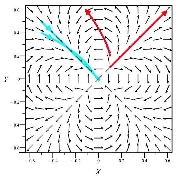
Figure 10: Particles which start in the repulsive zone are pushed to infinity both in the repulsive quadrant, and, after crossing over, also in the attractive quadrant. Particles which start from the attractive zone are in turn sucked into the hole. This behavior corresponds to the sign of the non-relativistic energy (V.10a).

and the circularly oscillating one in FIG.11.

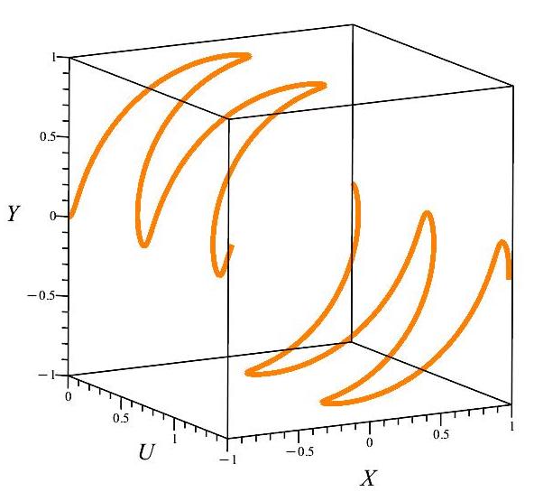
(a)

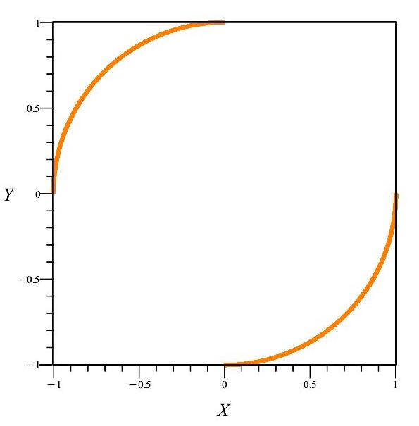
(b)

Figure 11: Numerically obtained periodic trajectories 11(a) in the ${\rm o}(2,1)$ symmetric but non-isotropic gravitational wave (V.8). 11(b) shows their projections onto the $X-Y$ plane, as seen also in FIG.12. The curves show two particles which start from $(1,0)$ resp. at $(-1,0)$ with zero initial velocity. The trajectories oscillate along quarters-of-a-circle.

The general behavior is summarised in FIG.12.

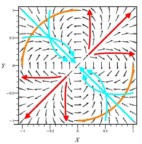
Figure 12: in the NE and SW quadrants the particle is pushed outwards to infinity whereas it is sucked into the origin in the NW and SE quadrants. Bounded zero-energy motions arise which oscillate in the attractive quadrant between the separation lines of the attractive and repulsives zones.

Analytic solutions can be found also.

We first inquire about radial motions. Putting $\theta=\theta_{0}=\mathop{\rm const.}\nolimits$ into (V.6)-(V.7) yields,

$$\frac{\;d^{2}R}{dU^{2}}-\frac{2\sin 2\theta_{0}}{R^{3}}=0\,{\quad\text{\small and}\quad}\frac{2\cos 2\theta_{0}}{R^{4}}=0\,.$$

The 2nd eqn requires $\cos 2\theta_{0}=0$, which implies,

$$\theta_{0}=(2\ell+1)\frac{\pi}{4}\,,\qquad\ell=0,\,1,\,2,\,3\,,$$ (V.17)

leaving us with,

$$\frac{d^{2}R}{dU^{2}}={\pm}\frac{2}{R^{3}}\,,$$ (V.18)

where the sign is positive in the repulsive, $\ell=0,\,2$ case and is negative in the attractive, $\ell=1,\,3$ one. Thus for $\ell$ pair the particle is expulsed to infinity along the “crest”, and for $\ell$ odd it is sucked into the origin along the “bottom valley” which correspond to the maximally repulsive or maximally attractive directions in FIGs. 8 and 9. The solution of the familiar inverse-cube force equation AFF ; DBKP ; DHP2 ; ScalingZCEH is,

$$R(U)=\sqrt{(V_{0}U+R_{0})^{2}\pm\frac{2U^{2}}{R_{0}^{2}}}\,,$$ (V.19)

where $R_{0}>0$ and $V_{0}$ are the initial position resp. the initial velocity along the diagonal. $V_{0}<0$ means falling towards the origin, and $V_{0}>0$ moving outwards. Starting in the repulsive quadrant we have the plus sign and the particle can not reach the origin. In the attractive quadrant the motion is directed towards the origin; the solution becoming imaginary indicates that the particle has fallen into the hole.

The equations (V.6)-(V.7) admit also exact circular, analytic solutions. Let us indeed fix the radius, $R(U)=R_{0}=\mathop{\rm const.}\nolimits$ which reduces (V.6)-(V.7) to,

$$\left(\frac{d\theta}{dU}\right)^{2}+\frac{2}{R_{0}^{4}}\,\sin 2\theta=0\,,\quad\frac{\,d^{2}\theta}{dU^{2}}+\frac{2}{R_{0}^{4}}\,\cos 2\theta=0\,.$$ (V.20)

Deriving the first eqn. by $U$ we get

$$\frac{d\theta}{dU}\left(\frac{\,d^{2}\theta}{dU^{2}}+\frac{2C_{2}}{R_{0}^{4}}\,\cos 2\theta\right)=0$$

which is an identity when the 2nd equation is satisfied. The first equation in (V.20) then implies that

$$\frac{d\theta}{dU}=\big{(}\frac{2}{R_{0}^{2}}\big{)}^{1/2}\,\sqrt{-\sin 2\theta}=0\,,$$ (V.21)

which admits real solutions when the sin is negative i.e. in the quadrants $\pi/2\leq\theta\pi$ and $3\pi/2\leq\theta 2\pi$ and is then solved in terms of elliptic integrals EllipticInt ,

$$\theta(U)=-\frac{1}{2}\arcsin\left\{\mathrm{JacobiCN}^{2}\left[\frac{2}{R_{0}^{2}}(U+D),\frac{\sqrt{2}}{2}\right]\right\}\,,$$ (V.22)

where $D$ is an integration constant. This formula can also be verified directly and is plotted in FIG.13 to be compared with the numerical solution in FIG.11).

This solution has zero-energy. Conversely Sundaram , for vanishing energy ${\cal E}=0$ the conserved quantity generated by dilations, (V.10b) implies $R=R_{0}=\mathop{\rm const.}\nolimits$, (V.14). Then (V.2a) becomes (V.15) which for $R=R_{0}$ is (V.21) that we have just solved. In conclusion, ${\rm o}(2,1)$ symmetry implies, for zero energy, motion on (part of) a circle.

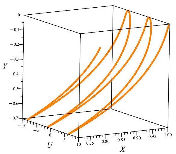
Figure 13: The analytic solution obtained in terms of elliptic integrals describes periodic motion along a circular arc confined into the attractive quadrant $\pi/2<\theta<\pi$, consistently with the numerical solutions in FIG. 11 and 14.

Restoring the radius in the equations shows that the period increases proportionally to the its square, $R_{0}^{2}$,

$$\Delta U=R_{0}^{2}\frac{4K}{\sqrt{2C_{2}}}\;\Rightarrow\;\Delta U\propto R_{0}^{2}\,,$$ (V.23)

as seen in FIG. 14.

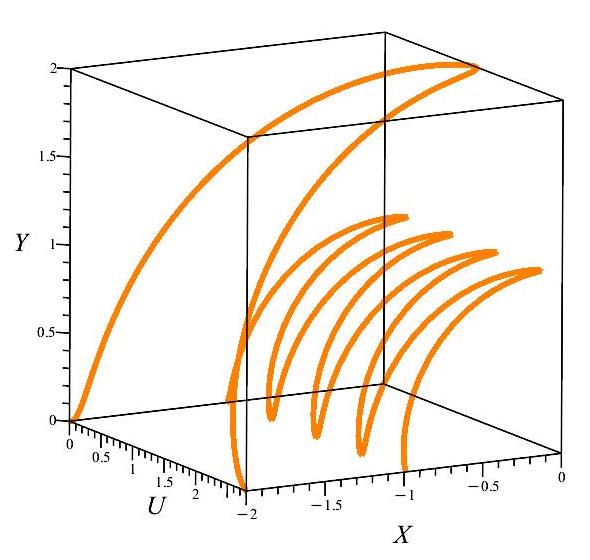
(a)

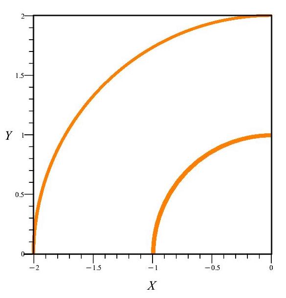
(b)

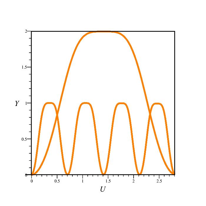
(c)

Figure 14: FIG. 14(a) shows the trajectories of two particles initially at rest on the separation line of the repulsive and attractive quadrants at $(1,0)$ and at $(2,0)$, respectively. The projections in FIG. 14(b) into the $X-Y$ plane follow quarter-of-circle arcs with radiuses $R_{0}=1$ and $R_{0}=2$, respectively. The projection into the $Y-U$ plane in FIG. 14(c), shows clearly that the period for $R_{0}=2$ is four times that for $R_{0}=1$, consistently with (V.23).

Inserting $\theta(U)$ from (V.22) into the conserved Casimir (V.5) we get, for $C_{1}=0$,

$$J^{2}=2\,\mathrm{JacobiCN}^{2}\left[\frac{2}{R_{0}^{2}}(U+C),\frac{\sqrt{2}}{2}\right]+\mathop{\rm const.}\nolimits$$ (V.24)

On the other hand, the angular momentum for (V.22) is

$${J}=\vec{R}\times\vec{V} = \,\mathrm{JacobiCN}\left[\frac{2}{R_{0}^{2}}(U+C),\frac{\sqrt{2}}{2}\right]\,.$$ (V.25)

whose square fixes the constant in (V.24) to vanish. The length of (V.25) thus oscillates as shown in FIG.15, consistently with the breaking of the axial symmetry.

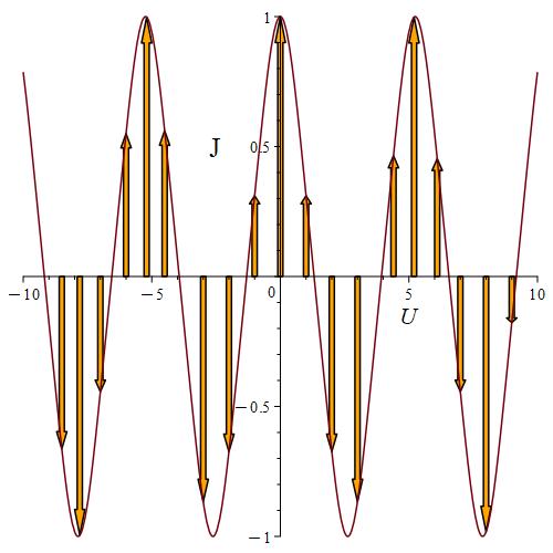
Figure 15: In the anisotropic metric (V.8) in FIG.8, the orbital angular momentum ${J}$ in (V.25) is not conserved: for the circular periodic motion found for zero energy, for example, its length oscillates. The direction of the oscillations seen in FIGs.11 and 14 corresponds to the sign of the angular momentum, with the turning point corresponding to the zeros of the angular momentum.

V.1 Approximate sandwich waves

Returning to gravitational waves, we mention that in realistic situations they are (approximate) sandwich waves Hawking ; BoPi89 ; Zhang:2017rno ; Zhang:2017geq ; Steinbauer1997 ; Podolsky:1998in ; PodSB ; Zhang:2017jma ; SBComment , obtained by inserting the profile (IV.5) into a “Gaussian envelope”,

$$ds_{Gauss}^{2}=dX^{2}+dY^{2}+2dUdV-2e^{-\lambda U^{2}}\left(\frac{C_{1}(X^{2}-Y^{2})+2C_{2}XY}{R^{4}}\right)dU^{2}.$$ (V.26)

The metric is still a vacuum however the $U$-dependent prefactor breaks the ${\rm O}(2,1)$ symmetry. In the (approximate) wave-zone it behaves as a “spike” — i.e., a narrow vacuum wave, whose sign alternates depending on the direction, shown in FIG.16.

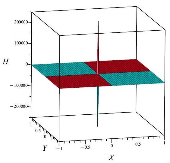
Figure 16: Putting the wave (V.8) into a Gaussian enveloppe, (V.26), yields, for large $\lambda$, a spike whose sign alternates at every quarter of the circle.

We found no analytic solutions, but numerical calculations indicate that particles at rest in the (approximate) before zone (See Hawking ; BoPi89 ; Zhang:2017rno ; Zhang:2017geq ; EZHrev for the terminology). fly apart with constant velocities in the after-zone i.e., after the gravitational wave has passed, as seen in FIGs.17 and 18 : we get the velocity effect Grishchuk1989 ; Zhang:2018srn .

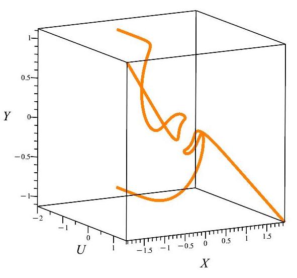
(a)

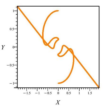
(b)

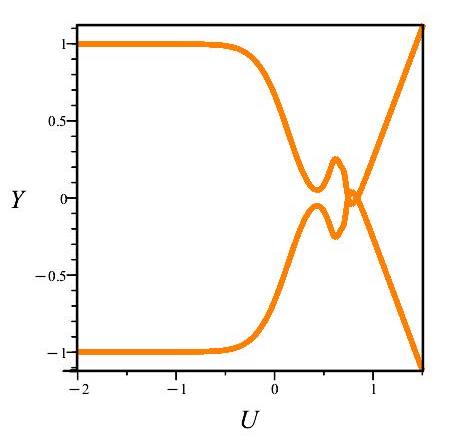
(c)

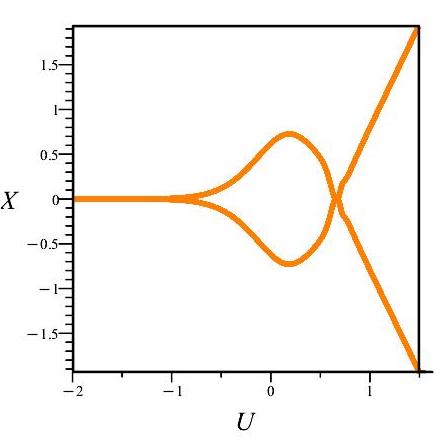
(d)

Figure 17: FIG. 17(a): $3d$ trajectories of two particles at rest at initial positions $({\bf 1,0})$ and $(\bf{-1,0})$ in the (approximate) before zone in the gravitational wave spacetime (V.26). The wave has a Gaussian profile. Their projections of the trajectories into the $X-Y$, $U-Y$ and $U-X$ planes are shown in FIGs.17(b)-17(c)-17(d). Both particles perform complicated motion in the wave zone before escaping with constant velocities after the gravitational wave has passed.

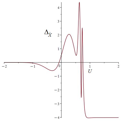
Figure 18: Velocity effect Grishchuk1989 ; Zhang:2018srn for the Gaussian profile: after violent motion in the short wave zone, the particles escape with non-zero constant velocity.

VI History: from Arnold through Newton, back to Galilei

The zero - energy motions which oscillate along quarter-of-circles in the attractive zone between the separation lines of the attractive and repulsive quarters have indeed quite remarkable ancestry. Let’s proceed backwards in history.

We start with noting that our equations (V.20) are reminiscent of studying planetary motion making use of the Bohlin-Arnold duality between harmonic oscillators and the Kepler problem Bohlin ; Arnold ; ZHArnold . Eqns. #(8.3) in ZHArnold which assume circular trajectories are (apart of circular motion in the usual $r^{-1}$ potential) consistent when the force is inversely proportional to the fifth power of the distance from the sun,

$$\text{force}\;\propto\;-\frac{1}{r^{5}}\,.$$ (VI.1)

This was known already by Newton, who, in his Principia, wondered: – What force laws do allow for circular trajectories ? And he found, using geometrical techniques, that (in addition to $r^{-2}$) one can have also (VI.1). See Principia vol. I Proposition VII. Problem II, where the proof is left as an exercise.

Yet another intriguing feature is that both our circular solution in sec.V and the parabolic trajectory of the 1680 comet (proved by Newton in his Principia Principia , Book III Proposition XLI, Problem XXI) have, just like our circular one found above, zero energy which separate bounded and unbounded motions. Even more incredibly, FIG.4 in Galilei’s “Dialogo” Dialogo , written before Newton was even born, suggests such a circular motion which would pass through the center of the Earth.

Returning to our circularly oscillating motions in sect.V we note that they do not enter into the Bohlin-Arnold framework. Let us explain. The clue is that the Bohlin-Arnold trick Bohlin ; Arnold is based on a duality between two central potentials proportional to $r^{a}$ and $r^{A}$, respectively. They are duals when the constraint

$$\left(1+\frac{a}{2}\right)\left(1+\frac{A}{2}\right)=1$$ (VI.2)

is satisfied; then motion in the $r^{a}$ and in the $r^{A}$ potentials can be swapped into each other.

The newtonian potential corresponds, for example, to $a=-1$; its dual has therefore $A=2$ i.e., that of an isotropic harmonic oscillator. This duality swaps also the dynamical symmetries of the oscillator with the Runge-Lenz vector-induced one of planetary motion. Working for simplicity in the plane using complex coordinates, $\zeta=\xi+i\eta$ for the oscillator and $z=x+iy$ for the Kepler problem, the corresponding Levi-Civita - Bohlin - Arnold map LeviCivita ; Bohlin ; Arnold ; Nersessian ; ZHArnold ,

$$z=\left(\zeta+\frac{1}{\zeta}\right)^{2}$$ (VI.3)

interchanges also those dynamical symmetries Berard . The potential of the inverse-5 force (VI.1) is in turn self-dual, $a=A=-4$.

However the inverse square potential, which is what we are interested in in this paper, does not enter the Bohlin-Arnold duality because it has no dual: the constraint (VI.2) can not be satisfied for $a=-2$. It is therefore a remarkable tour de force that Sundaram et al Sundaram could extend the Bohlin-Arnold duality to that case.

VII Summary and discussions

In this paper we study conformally related vacuum gravitational waves and their associated symmetries by using a special Möbius conformal transformation (II.7)-(II.8). The vacuum condition is preserved by eliminating the additional non-vacuum oscillator term (II.4) Masterov ; ZZH2022 . The resulting GW is in general different from the original one. The transformation (II.7)-(II.8) carries a global GW into an (approximate) sandwich wave, as illustrated by LPP GW and CPP GW which exemplify the memory effect ZelPol ; Braginsky1985 ; Grishchuk1989 ; Zhang:2017rno ; Zhang:2017geq ; EZHrev .

A vacuum GW can also be invariant under the special Möbius conformal transformation (II.7)-(II.8) when it has an ${\rm O}(2,1)$ symmetry. The remarkable efficiency of this symmetry is that its generators act on the radial variable only, therefore they apply equally well to anisotropis systems.

The particularly interesting example originating in molecular physics Camblong:2001zt but applied here in the gravitational context by using the Bargmann framework DBKP ; Eisenhart ; DGH91 is studied in some detail. It has the form of the inverse-square potential AFF whose rôle played in black-hole physics has been noticed before Camblong:2003mz in the isotropic case.

For the polar-molecular application, (V.1) the familiar rotational symmetry is broken by an angle-dependent coefficient which makes it anisotropic: it alternates between repulsive and attractive at every quarter-of-a circle, see (V.8). The particle is accordingly being pushed out to infinity or attracted towards the singularity at the origin, depending on the sign of the energy in the underlying non-relativistic problem. The behavior is reminiscent of that in the Kepler problem.

Bounded motion arise in the attractive quadrant, with the particle oscillates along quarter-of-circle between the lines which separate the attractive and repulsive quadrants.

Analytic solutions were found for escaping or incoming radial motion along the “crests” or “valley bottoms" which correponds to the usual inverse-square potential with repulsive or attractive sign.

The anisotropy breaks the rotational symmetry : the length of the angular momentum (V.25) oscillates, as shown in FIG.15 in the periodic case.

The analytic periodic motions in the attractive zone show remarkable historical analogies, recounted in sec. VI by proceeding backwards in time.

Approximately sandwich waves are obtained by putting the profile into a Gaussian envelop. No analytic solutions are found but we observe instead the (approximate) velocity effect Grishchuk1989 ; Zhang:2018srn .

The rôle played by the inverse-square potential in black-hole physics has been noticed before Claus , for the isotropic Reissner-Nordström solution Camblong:2003mz . The anisotropic metric (V.8), which seems to have escaped attention so far, is a pp wave which resembles that near the “Dirac String” in the Lorentzian Taub-NUT metric Gibbons:2006gx ; Holzegel:2006gn ; GWG .

- (1) H. W. Brinkmann, “Einstein spaces which are mapped conformally on each other,” Math. Ann. 94 (1925), 119-145 doi:10.1007/BF01208647
- (2) C. Duval, G. W. Gibbons and P. Horvathy, “Celestial mechanics, conformal structures and gravitational waves,” Phys. Rev. D 43 (1991), 3907-3922 doi:10.1103/PhysRevD.43.3907 [arXiv:hep-th/0512188 [hep-th]].
- (3) V. Bargmann, “On Unitary ray representations of continuous groups,” Annals Math. 59 1 (1954).
- (4) C. Duval, G. Burdet, H. P. Künzle and M. Perrin, “Bargmann structures and Newton-Cartan theory", Phys. Rev. D 31 (1985) 1841.
- (5) G. Burdet, C. Duval and M. Perrin, “Time Dependent Quantum Systems and Chronoprojective Geometry,” Lett. Math. Phys. 10 (1985), 255-262 doi:10.1007/BF00420564
- (6) L. P. Eisenhart, “Dynamical trajectories and geodesics", Annals Math. 30 591-606 (1928).
- (7) Ya. B. Zel’dovich and A. G. Polnarev, “Radiation of gravitational waves by a cluster of superdense stars," Astron. Zh. 51, 30 (1974) [Sov. Astron. 18 17 (1974)].
- (8) V. B. Braginsky and L. P. Grishchuk, “Kinematic Resonance and Memory Effect in Free Mass Gravitational Antennas,” Sov. Phys. JETP 62 (1985), 427-430
- (9) L. P. Grishchuk and A. G. Polnarev, “Gravitational wave pulses with ‘velocity coded memory’,” Sov. Phys. JETP 69 (1989), 653-657
- (10) J. Ehlers and W. Kundt, “Exact solutions of the gravitational field equations,” in Gravitation: An Introduction to Current Research, edited by L. Witten (Wiley, New York, London, 1962).
- (11) J-M. Souriau, “Ondes et radiations gravitationnelles,” Colloques Internationaux du CNRS No 220, pp. 243-256. Paris (1973).
- (12) M. Elbistan, P. M. Zhang and P. A. Horvathy, “Memory effect & Carroll symmetry, 50 years later,” Annals Phys. 459 (2023), 169535 doi:10.1016/j.aop.2023.169535
- (13) C. Duval, G. W. Gibbons, P. A. Horvathy and P. M. Zhang, “Carroll symmetry of plane gravitational waves,” Class. Quant. Grav. 34 (2017) no.17, 175003 doi:10.1088/1361-6382/aa7f62 [arXiv:1702.08284 [gr-qc]]. This paper draws heavily on Sou73 .
- (14) P. M. Zhang, C. Duval, G. W. Gibbons and P. A. Horvathy, “The Memory Effect for Plane Gravitational Waves,” Phys. Lett. B 772 (2017), 743-746 doi:10.1016/j.physletb.2017.07.050 [arXiv:1704.05997 [gr-qc]].
- (15) P. M. Zhang, C. Duval, G. W. Gibbons and P. A. Horvathy, “Soft gravitons and the memory effect for plane gravitational waves,” Phys. Rev. D 96 (2017) no.6, 064013 doi:10.1103/PhysRevD.96.064013 [arXiv:1705.01378 [gr-qc]].
- (16) P. M. Zhang, C. Duval, G. W. Gibbons and P. A. Horvathy, “Velocity Memory Effect for Polarized Gravitational Waves,” JCAP 05 (2018), 030 doi:10.1088/1475-7516/2018/05/030 [arXiv:1802.09061 [gr-qc]].
- (17) L. Marsot, “Planar Carrollean dynamics, and the Carroll quantum equation,” J. Geom. Phys. 179 (2022), 104574 doi:10.1016/j.geomphys.2022.104574 [arXiv:2110.08489 [math-ph]].
- (18) H. Bondi, F. A. E. Pirani and I. Robinson, “Gravitational waves in general relativity. 3. Exact plane waves,” Proc. Roy. Soc. Lond. A 251 (1959), 519-533 doi:10.1098/rspa.1959.0124
- (19) Sippel, R., Goenner, H. (1986). “Symmetry classes of pp-waves. General relativity and gravitation,” General Relativity and Gravitation 18 (1986), 1229-1243.
- (20) H. Stephani, D. Kramer, M. A. H. MacCallum, C. Hoenselaers and E. Herlt, “Exact solutions of Einstein’s field equations,” Cambridge Univ. Press (2003). doi:10.1017/CBO9780511535185
- (21) R. Maartens and S. D. Maharaj, “Conformal symmetries of pp waves,” Class. Quant. Grav. 8 (1991) 503. doi:10.1088/0264-9381/8/3/010.
- (22) A. J. Keane and B. O. J. Tupper, “Conformal symmetry classes for pp-wave spacetimes,” Class. Quant. Grav. 21 (2004), 2037 doi:10.1088/0264-9381/21/8/009 [arXiv:1308.1683 [gr-qc]].
- (23) M. Dunajski and R. Penrose, “Quantum state reduction, and Newtonian twistor theory,” Annals Phys. 451 (2023), 169243 doi:10.1016/j.aop.2023.169243 [arXiv:2203.08567 [gr-qc]].
- (24) M. Dunajski, “Equivalence principle, de-Sitter space, and cosmological twistors,” [arXiv:2304.08574 [gr-qc]].
- (25) U. Niederer, “The maximal kinematical invariance group of the harmonic oscillator,” Helv. Phys. Acta 46 (1973), 191-200 PRINT-72-4208.
- (26) S. Dhasmana, A. Sen and Z. K. Silagadze, “Equivalence of a harmonic oscillator to a free particle and Eisenhart lift,” Annals Phys. 434 (2021), 168623 doi:10.1016/j.aop.2021.168623 [arXiv:2106.09523 [quant-ph]].
- (27) A. Sen, B. K. Parida, S. Dhasmana and Z. K. Silagadze, “Eisenhart lift of Koopman-von Neumann mechanics,” J. Geom. Phys. 185 (2023), 104732 doi:10.1016/j.geomphys.2022.104732 [arXiv:2207.05073 [gr-qc]].
- (28) P. Zhang, Q. Zhao and P. A. Horvathy, “Gravitational waves and conformal time transformations,” Annals Phys. 440 (2022), 168833 doi:10.1016/j.aop.2022.168833 [arXiv:2112.09589 [gr-qc]].
- (29) G. W. Gibbons, “Dark Energy and the Schwarzian Derivative,” [arXiv:1403.5431 [hep-th]].
- (30) P. M. Zhang, M. Elbistan and P. A. Horvathy, “Particle motion in circularly polarized vacuum pp waves,” Class. Quant. Grav. 39 (2022) no.3, 035008 doi:10.1088/1361-6382/ac43d2 [arXiv:2108.00838 [gr-qc]].
- (31) M. Elbistan, “Circularly polarized periodic gravitational wave and the Pais-Uhlenbeck oscillator,” Nucl. Phys. B 980 (2022), 115846 doi:10.1016/j.nuclphysb.2022.115846 [arXiv:2203.02338 [gr-qc]].
- (32) I. Masterov and M. Masterova, “Coupling-constant metamorphosis in SL(2,R)-invariant systems,” J. Geom. Phys. 168 (2021), 104320 doi:10.1016/j.geomphys.2021.104320
- (33) H. E. Camblong, L. N. Epele, H. Fanchiotti and C. A. Garcia Canal, “Quantum anomaly in molecular physics,” Phys. Rev. Lett. 87 (2001), 220402 doi:10.1103/PhysRevLett.87.220402 [arXiv:hep-th/0106144 [hep-th]].
- (34) H. E. Camblong and C. R. Ordonez, “Anomaly in conformal quantum mechanics: From molecular physics to black holes,” Phys. Rev. D 68 (2003), 125013 doi:10.1103/PhysRevD.68.125013 [arXiv:hep-th/0303166 [hep-th]].
- (35) S. Moroz and R. Schmidt, “Nonrelativistic inverse square potential, scale anomaly, and complex extension,” Annals Phys. 325 (2010), 491-513 doi:10.1016/j.aop.2009.10.002 [arXiv:0909.3477 [hep-th]].
- (36) J. B. Achour, “Proper time reparametrization in cosmology: Möbius symmetry and Kodama charges,” JCAP 12 (2021) no.12, 005 doi:10.1088/1475-7516/2021/12/005 [arXiv:2103.10700 [gr-qc]].
- (37) G. W. Gibbons and S. W. Hawking, “Theory of the detection of short bursts of gravitational radiation,” Phys. Rev. D 4 (1971), 2191-2197 doi:10.1103/PhysRevD.4.2191
- (38) H. Bondi and F. A. E. Pirani, “Gravitational Waves in General Relativity. 13: Caustic Property of Plane Waves,” Proc. Roy. Soc. Lond. A 421 (1989) 395.
- (39) R. Steinbauer, “Geodesics and geodesic deviation for impulsive gravitational waves,” J. Math. Phys. 39 (1998), 2201-2212 doi:10.1063/1.532283 [arXiv:gr-qc/9710119 [gr-qc]].
- (40) J. Podolsky and K. Vesely, “New examples of sandwich gravitational waves and their impulsive limit,” Czech. J. Phys. 48 (1998), 871-878 doi:10.1023/A:1022869004605 [arXiv:gr-qc/9801054 [gr-qc]].
- (41) J. Podolsky and R. Steinbauer, “Geodesics in space-times with expanding impulsive gravitational waves,” Phys. Rev. D 67 (2003), 064013 doi:10.1103/PhysRevD.67.064013 [arXiv:gr-qc/0210007 [gr-qc]].
- (42) P. M. Zhang, C. Duval and P. A. Horvathy, “Memory Effect for Impulsive Gravitational Waves,” Class. Quant. Grav. 35 (2018) no.6, 065011 doi:10.1088/1361-6382/aaa987 [arXiv:1709.02299 [gr-qc]].
- (43) R. Steinbauer, “The memory effect in impulsive plane waves: comments, corrections, clarifications,” Class. Quant. Grav. 36 (2019) no.9, 098001 doi:10.1088/1361-6382/ab127d [arXiv:1811.10940 [gr-qc]].
- (44) K. Andrzejewski and S. Prencel, “Memory effect, conformal symmetry and gravitational plane waves,” Phys. Lett. B 782 (2018), 421-426 doi:10.1016/j.physletb.2018.05.072 [arXiv:1804.10979 [gr-qc]].
- (45) K. Andrzejewski and S. Prencel, “Niederer’s transformation, time-dependent oscillators and polarized gravitational waves,” doi:10.1088/1361-6382/ab2394 [arXiv:1810.06541 [gr-qc]].
- (46) P. A. M. Dirac, “New basis for cosmology,” Proc. Roy. Soc. Lond. A 165 (1938), 199-208 doi:10.1098/rspa.1938.0053
- (47) C.G. Torre, “Gravitational waves: just plane symmetry,” Gen. Relat. Gravit. 38, 653 (2006). arXiv:gr-qc/9907089
- (48) P. M. Zhang, M. Elbistan, G. W. Gibbons and P. A. Horvathy, “Sturm-Liouville and Carroll: at the heart of the memory effect,” Gen. Rel. Grav. 50 (2018) no.9, 107 doi:10.1007/s10714-018-2430-0 [arXiv:1803.09640 [gr-qc]].
- (49) M. Elbistan, P. M. Zhang, G. W. Gibbons and P. A. Horvathy, “Lukash plane waves, revisited,” JCAP 01 (2021), 052 doi:10.1088/1475-7516/2021/01/052 [arXiv:2008.07801 [gr-qc]].
- (50) M. Brdicka, “On Gravitational Waves,” Proc. Roy. Irish Acad. 54A (1951) 137.
- (51) M. Elbistan, N. Dimakis, K. Andrzejewski, P. A. Horvathy, P. Kosínski and P. M. Zhang, “Conformal symmetries and integrals of the motion in pp waves with external electromagnetic fields,” Annals Phys. 418 (2020), 168180 doi:10.1016/j.aop.2020.168180 [arXiv:2003.07649 [gr-qc]].
- (52) R. Jackiw, “Introducing scale symmetry,” Phys. Today 25N1 (1972), 23-27 doi:10.1063/1.3070673 C. R. Hagen, “Scale and conformal transformations in galilean-covariant field theory,” Phys. Rev. D 5 (1972), 377-388 doi:10.1103/PhysRevD.5.377 U. Niederer, “The maximal kinematical invariance group of the free Schrodinger equation,” Helv. Phys. Acta 45 (1972), 802-810 doi:10.5169/seals-114417
- (53) C. Duval, P. A. Horvathy and L. Palla, “Conformal Properties of Chern-Simons Vortices in External Fields,” Phys. Rev. D 50 (1994), 6658-6661 doi:10.1103/PhysRevD.50.6658 [arXiv:hep-th/9404047 [hep-th]].
- (54) S. Dhasmana, A. Sen and Z. K. Silagadze, “Equivalence of a harmonic oscillator to a free particle and Eisenhart lift,” Annals Phys. 434 (2021), 168623 doi:10.1016/j.aop.2021.168623 [arXiv:2106.09523 [quant-ph]].
- (55) R. Jackiw and S. Y. Pi, “Soliton Solutions to the Gauged Nonlinear Schrodinger Equation on the Plane,” Phys. Rev. Lett. 64 (1990), 2969-2972 doi:10.1103/PhysRevLett.64.2969 R. Jackiw and S. Y. Pi, “Classical and quantal nonrelativistic Chern-Simons theory,” Phys. Rev. D 42 (1990), 3500 [erratum: Phys. Rev. D 48 (1993), 3929] doi:10.1103/PhysRevD.42.3500
- (56) C. Duval, P. A. Horvathy and L. Palla, “Conformal symmetry of the coupled Chern-Simons and gauged nonlinear Schrodinger equations,” Phys. Lett. B 325 (1994), 39-44 doi:10.1016/0370-2693(94)90068-X [arXiv:hep-th/9401065 [hep-th]].
- (57) C. G. J. Jacobi, “Vorlesungen über Dynamik.” Univ. Königsberg 1842-43. Herausg. A. Clebsch. Zweite ausg. C. G. J. Jacobi’s Gesammelte Werke. Supplementband. Herausg. E. Lottner. Berlin Reimer (1884). An english translation is available as Jacobi’s Lectures on Dynamics, 2nd edition, Texts and Readings in Mathematics, https://doi.org/10.1007/978-93-86279-62-0, Hindustan Book Agency Gurgaon.
- (58) V. de Alfaro, S. Fubini and G. Furlan, “Conformal Invariance in Quantum Mechanics,” Nuovo Cim. A 34 (1976), 569 doi:10.1007/BF02785666
- (59) P. M. Zhang, M. Cariglia, M. Elbistan and P. A. Horvathy, “Scaling and conformal symmetries for plane gravitational waves,” J. Math. Phys. 61 (2020) no.2, 022502 doi:10.1063/1.5136078 [arXiv:1905.08661 [gr-qc]].
- (60) V. Efimov, “Energy levels of three resonantly interacting particles,” Nucl. Phys. A 210 (1973), 157-188 doi:10.1016/0375-9474(73)90510-1
- (61) P. Claus, M. Derix, R. Kallosh, J. Kumar, P. K. Townsend and A. Van Proeyen, “Black holes and superconformal mechanics,” Phys. Rev. Lett. 81 (1998), 4553-4556 doi:10.1103/PhysRevLett.81.4553 [arXiv:hep-th/9804177 [hep-th]].
- (62) S. S. Gubser, I. R. Klebanov and A. M. Polyakov, “Gauge theory correlators from noncritical string theory,” Phys. Lett. B 428 (1998), 105-114 doi:10.1016/S0370-2693(98)00377-3 [arXiv:hep-th/9802109 [hep-th]].
- (63) E. Witten, “Anti-de Sitter space and holography,” Adv. Theor. Math. Phys. 2 (1998), 253-291 doi:10.4310/ATMP.1998.v2.n2.a2 [arXiv:hep-th/9802150 [hep-th]].
- (64) R. Jackiw, “Dynamical Symmetry of the Magnetic Monopole,” Annals Phys. 129 (1980), 183 doi:10.1016/0003-4916(80)90295-X
- (65) R. Jackiw, “Dynamical Symmetry of the Magnetic Vortex,” Annals Phys. 201 (1990), 83-116 doi:10.1016/0003-4916(90)90354-Q
- (66) Prasolov, V. V., Solov_ev, I. P. “Elliptic functions and elliptic integrals,” American Mathematical Soc., 1997, Vol. 170.
- (67) Sriram Sundaram, C. P. Burgess, D. H. J. O’Dell, “Duality between the quantum inverted harmonic oscillator and inverse square potentials,” e-print: [2402.13909 [quant-ph]]
- (68) V. I. Arnold: Huygens & Barrow, Newton & Hook. Birkhäuser (1990).
- (69) M. K. Bohlin, “Note sur le problème des deux corps et sur une intégration nouvelle dans le problème des trois corps,” Bull. Astron. 28, 113 (1911)
- (70) P. M. Zhang and P. Horvathy, “The laws of planetary motion, derived from those of a harmonic oscillator (following Arnold),” Physics Education (India) [arXiv:1404.2265v3 [physics.class-ph]]
- (71) I. S. Newton, Philosophia Naturalis Pricipia Mathematica. London: Royal Society of London (1686), translated by A. Motte as Sir Isaac Newton’s Mathematical Principles of Natural Philosphy and his System of the World (1729). Translation revised by F. Cajori, Berkeley: University of California Press (1946).
- (72) Galileo Galilei, Dialogo sopra i due massimi sistemi del mondo, Firenze, (1632).
- (73) A. Nersessian, V. Ter-Antonian and M. M. Tsulaia, “A Note on quantum Bohlin transformation,” Mod. Phys. Lett. A 11 (1996) 1605 doi:10.1142/S0217732396001600 [hep-th/9604197].
- (74) T. Levi-Civita: “Sur la résolution qualitative du problème resteint des trois corps,” Acta Math. 30, 305-327 (1906), Opere Matematiche, Vol. 2, p. 419. Bologna (1956).
- (75) Y. Grandati, A. Berard, H. Mohrbach, “Bohlin-Arnold-Vassiliev’s duality and conserved quantities,” e-Print: 0803.2610 [math-ph]
- (76) G. W. Gibbons and G. Holzegel, “The Positive mass and isoperimetric inequalities for axisymmetric black holes in four and five dimensions,” Class. Quant. Grav. 23 (2006), 6459-6478 doi:10.1088/0264-9381/23/22/022 [arXiv:gr-qc/0606116 [gr-qc]].
- (77) G. Holzegel, “A Note on the instability of Lorentzian Taub-NUT-space,” Class. Quant. Grav. 23 (2006), 3951-3962 doi:10.1088/0264-9381/23/11/017 [arXiv:gr-qc/0602045 [gr-qc]].
- (78) G. W. Gibbons, private communiction (2024)