Dynamical observation of non-trivial doublon formation using a quantum computer

Abstract

Dynamical formation of doublons or onsite repulsively bound pairs of particles on a lattice is a highly non-trivial phenomenon. In this work we show the signatures of doublon formation in a quantum computing experiment by simulating the continuous time quantum walk in the framework of the one dimensional extended Fermi-Hubbard model. By considering two up-component and one down-component particles initially created at the three neighbouring sites at the middle of the lattice and allowing intra- (inter-) component nearest neighbour (onsite) interactions we show the formation a stable onsite doublon in the quantum walk. The probability of such doublon formation is more (less) if the hopping strength of the down particle is weaker (stronger) compared to the up particle. On the contrary, for an initial doublon along with a free up particle, the stability of the doublon is more prominent than the doublon dissociation in the dynamics irrespective of the hopping asymmetry between the two components. We first numerically obtain the signatures of the stable doublon formation in the dynamics and then observe them using Noisy Intermediate-Scale Quantum (NISQ) devices.

Introduction.- Dynamics of interacting many-body systems following a sudden quench of system parameters reveals fascinating phenomena in condensed matter Bloch et al. (2008); Moeckel and Kehrein (2010); Polkovnikov et al. (2011). Interactions along with particle statistics and lattice geometries are known to play crucial roles in establishing non-trivial scenarios in the dynamics which are otherwise absent in systems at equilibrium. One such phenomenon is the formation of doublons that are the repulsively bound onsite pairs of constituent particles formed due to strong inter-particle interactions. Although the concept of doublons was originally discussed in the context of Hubbard model Hubbard and Flowers (1963); Yang (1989), recent progress in the field of ultracold atoms in optical lattices have enabled the observation of stable doublons of bosonic particles  Winkler et al. (2006). Subsequently doublons have been observed in the context of several bosonic and fermionic Hubbard models Jördens et al. (2008); Strohmaier et al. (2010); Greif et al. (2011); Meinert et al. (2013); Jürgensen et al. (2014); Xia et al. (2015); Covey et al. (2016); de Hond et al. (2022) and their dynamical properties have been studied in recent years Petrosyan et al. (2007); Khomeriki et al. (2010); Hofmann and Potthoff (2012); Kolovsky et al. (2012); Longhi and Della Valle (2012); Santos and Dykman (2012); Chudnovskiy et al. (2012); Longhi and Della Valle (2013); Boschi et al. (2014); Wiater et al. (2017); Gärttner et al. (2019).

While the study of controllable formation of doublons and their stability in many-body systems remain challenging both theoretically and experimentally, the quench dynamics of few interacting particles or the continuous time quantum walk (QW) offers a suitable platform to realise such phenomena in the simplest possible way Kempe (2003); Venegas-Andraca (2012). In this context, it has been well understood that a pair of particles (bosons or fermions of two different spins) when initialized on a particular site form a stable doublon in the QW due to strong onsite interaction. However, when initiated at the nearest neighbour (NN) sites, a doublon is not formed as strong repulsion between the constituents prohibits the overlap of their wavefunctions Preiss et al. (2015); Lahini et al. (2012). This question remained open until the recent prediction of stable onsite doublon formation in the QW of initially non-local bosons in the QW of two-component bosons Giri et al. (2022). However, the observation of such non-trivial doublon remains challenging due to the complexity of the model involved.

Recently, quantum computers have become very useful tool to simulate the dynamics of condensed matter systems and observe various physical phenomena Smith et al. (2019); Motta et al. (2020); Vovrosh and Knolle (2021); Sun et al. (2021); Kamakari et al. (2022); Chen et al. (2023); Koh et al. (2023a); Hoke et al. (2023); Shen et al. (2023). Several quantum computing experiments have been performed in the context of condensed matter physics using such NISQ devices which includes topological phases Azses et al. (2020); Smith et al. (2022); Koh et al. (2022a, b); Tan et al. (2023); Koh et al. (2023b), Floquet systems Mei et al. (2020); Mi et al. (2022); Harle et al. (2023), Fermi-Hubbard models Arute et al. (2020); Anselme Martin et al. (2022); Stanisic et al. (2022), spin systems Smith et al. (2019); Sun et al. (2021); Wang et al. (2023); Rosenberg et al. (2023), quantum scar Chen et al. (2022), non-hermitian physics Shen et al. (2023) etc. However, the operations involving qubits or two-level systems in such quantum devices play a real bottleneck for the simulation of the dynamics of bosonic Hamiltonians involving finite short-range interactions and hence the observation of the non-trivial onsite doublons. To counter such difficulties, it is essential to consider systems of fermions whose dynamics can be simulated using the exiting quantum computers.

In this work, we simulate the QW of two-component fermions ($\uparrow$ and $\downarrow$) and observe the dynamical formation of a stable doublon in a quantum computing experiment. By considering an initial state of three nearest neighbour fermions in a one dimensional chain, we show that a stable onsite doublon ($\uparrow\downarrow$ pair) is formed due to the competition between the onsite inter-particle interaction and nearest-neighbour (NN) intra-particle interaction. We find that the formation, dissociation, and stability of such doublon strongly depend on the hopping asymmetry between the two components, interplay between interactions and the initial configuration considered. We first numerically establish the formation of this non-trivial doublon and then perform a digital quantum circuit implementation in the framework of the Fermi-Hubbard model on NISQ devices.

Model and approach.- The system of two component fermions possessing onsite and NN interaction in one dimension is described by the extended Hubbard model which is given by the Hamiltonian

$$\begin{split}\hat{H}=\sum_{j,\sigma={\uparrow,\downarrow}}-J_{\sigma}(\hat{a}_{j,\sigma}^{\dagger}\hat{a}_{j+1,\sigma}&+\text{H.c.})+\sum_{j,\sigma}V_{\sigma\sigma^{\prime}}\hat{n}_{j,\sigma}\hat{n}_{j+1,\sigma^{\prime}}\\ &+U_{\uparrow\downarrow}\sum_{j}\hat{n}_{j,\uparrow}\hat{n}_{j,\downarrow},\end{split}$$ (1)

where ${\hat{a}^{\dagger}}_{j,\sigma}$$(\hat{a}_{j,\sigma})$ are the creation (annihilation) operator for two types of fermions denoted by $\sigma=\uparrow,\downarrow$ and $\hat{n}_{j,\sigma}=\hat{a}^{\dagger}_{j,\sigma}\hat{a}_{j,\sigma}$ is the particle number at the $j^{th}$ lattice site. $J_{\sigma}$ is the NN hopping strength of the particles, $V_{\sigma\sigma^{\prime}}$ and $U_{\uparrow\downarrow}$ are the NN and inter-component onsite interaction strengths respectively. We define $\delta=\frac{J_{\downarrow}}{J_{\uparrow}}$ as the hopping or mass imbalance between the up and down particles.

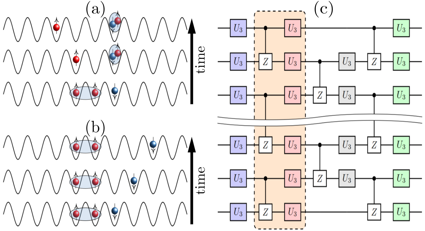
Figure 1: Show the short-time evolution of the initial state $|\psi(0)\rangle=\hat{a}_{-1,\uparrow}^{\dagger}\hat{a}_{0,\uparrow}^{\dagger}\hat{a}_{1,\downarrow}^{\dagger}|vac\rangle$. Two possible energy conserving time evolution processes are shown in (a) and (b). (c) shows the recompiled circuit, consisting of an alternative single-qubit $U_{3}$ layer and two-qubit control-Z layer. A gate round consists of a single layer of single-qubit gate and a single layer of two-qubit gate shown in the dashed box.

The quantum state at time $t\neq 0$ is determined from the solution of the time-dependent Schrodinger equation, $|\psi(t)\rangle=e^{-i\hat{H}t}|\psi(0)\rangle$, where $|\psi(0)\rangle$ is the initial state. Our numerical study is based on the time evolved block decimation (TEBD)  Vidal (2003, 2004) approach using the OSMPS library Wall and Carr (2012); Jaschke et al. (2018) by considering systems of size $L=51$ sites. For the quantum circuit implementation, we consider a limited number of qubits and further compare the results with the data obtained using the exact diagonalization (ED) method for an equivalent system. Although we restrict ourselves to smaller system sizes and short-time dynamics in our quantum computing experiment, we are able to capture important physics using certain kinds of error mitigation and circuit optimization techniques which will be discussed in the following.

Results.- The QW is studied by considering an initial state of two $\uparrow$ and one $\downarrow$ particles located at the three consecutive sites such that the two $\uparrow$ particle are in the NN sites and the $\downarrow$ is on the adjacent site on the right of the right $\uparrow$ particle as depicted in Fig. 1(a). The initial state corresponding to this configuration is given as $|\psi(0)\rangle=\hat{a}_{-1,\uparrow}^{\dagger}\hat{a}_{0,\uparrow}^{\dagger}\hat{a}_{1,\downarrow}^{\dagger}|vac\rangle$. For this choice of the initial state, although $U_{\uparrow\downarrow}$ and both $V_{\uparrow\uparrow}$ and $V_{\uparrow\downarrow}$ terms are allowed, we assume $V_{\uparrow\downarrow}=0$ to capture the desired physics due to the competing interactions. From here onwards we denote $U_{\uparrow\downarrow}$ and $V_{\uparrow\uparrow}$ as $U$ and $V$ respectively. We consider a stronger NN interaction $V=10$ and vary $U$ to study their combined effect on the dynamics. When $U=0$, it is expected that the two $\uparrow$ particles form a repulsively bound NN pair ($\uparrow\uparrow$) at their initial position Fukuhara et al. (2013); Li et al. (2020) and move together whereas the down particle perform independent particle QW. However, as $U$ becomes finite and comparable with $V$ (i.e. $U\sim V$), we obtain finite probabilities of both onsite doublon along with an NN pair ($\uparrow\uparrow$) in the dynamics for equal hopping strengths of both the components (i.e. $\delta=1$). This behaviour can be quantified by comparing the probabilities of the doublon and the NN pair ($\uparrow\uparrow$) formation defined as

$$P_{\uparrow\downarrow}=\sum_{i}^{L}\langle\hat{n}_{i,\uparrow}\hat{n}_{i,\downarrow}\rangle\ \ \text{and}\ \ P_{\uparrow\uparrow}=\sum_{i}^{L-1}\langle\hat{n}_{i,\uparrow}\hat{n}_{i+1,\uparrow}\rangle$$ (2)

respectively.

In Fig. 2(a), we plot the time evolution of $P_{\uparrow\downarrow}$ (filled diamonds) and $P_{\uparrow\uparrow}$ (empty diamonds) for $\delta=1$ and $U=V=10$ which saturate to finite values close to $0.5$. The almost equal probabilities for both the $\uparrow\downarrow$ and $\uparrow\uparrow$ bound pairs is due to the almost equal energies of both the states at $U=V$. However, introducing a finite hopping imbalance i.e. $\delta<1$, $P_{\uparrow\downarrow}$ (filled symbols) clearly dominates over $P_{\downarrow\downarrow}$ (empty symbols) in the time evolution which are shown as blue squares for $\delta=0.4$ and red circles for $\delta=0.2$ respectively. This indicates that when the hopping imbalance is stronger (i.e. $\delta<<1$), the $\uparrow\uparrow$ pair tends to dissociate completely and a stable onsite doublon ($\uparrow\downarrow$) is formed in the QW. To quantify this behaviour further, we plot the saturated values of $P_{\uparrow\downarrow}$ (filled circles) and $P_{\uparrow\uparrow}$ (empty circles) after $t=10(J_{\uparrow}^{-1})$ in the time evolution as a function of $U$ for $V=10$ and $\delta=0.2$ in Fig. 2(b). The figure depicts that initially for $U=0$, $P_{\uparrow\uparrow}\sim 1$ and as $U$ increases and becomes $U\sim V=10$, $P_{\uparrow\uparrow}$ reaches a minimum value close to zero and at the same time $P_{\uparrow\downarrow}$ becomes maximum, indicating a stable doublon formation and dissociation of the NN pair ($\uparrow\uparrow$). Further increase in the value of $U$ leads to the stability of the NN pair ($\uparrow\uparrow$) state as the energy of the doublon state is off resonant to the NN pair ($\uparrow\uparrow$) state which prohibits an NN pair ($\uparrow\uparrow$) breaking - a situation similar to the case when $U<V$.

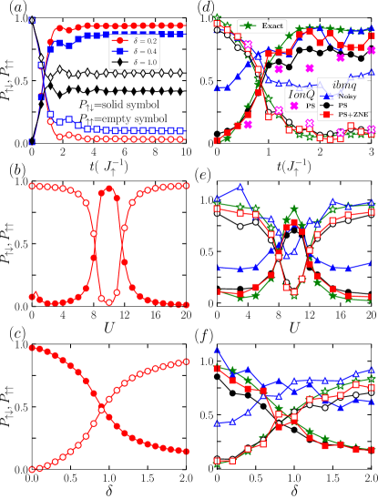
Figure 2: Left panel shows the results from the classical simulation with $L=51$. (a) $P_{\uparrow\downarrow}$ and $P_{\uparrow\uparrow}$ are plotted as a function of time at the resonance condition ($V=U=10$) for different values of hopping imbalance $\delta$. (b) $P_{\uparrow\downarrow}$ and $P_{\uparrow\uparrow}$ are plotted against $U$ for $\delta=0.2$ and $V=10$ at a particular time $t=10J_{\uparrow}^{-1}$. (c) $P_{\uparrow\downarrow}$ and $P_{\uparrow\uparrow}$ plotted as a function of $\delta$, for $U=V=10$ at time $t=10J_{\uparrow}^{-1}$. The right panel shows the results from the digital quantum simulation for $7$ lattice sites and short-time dynamics. (d) Shows the $P_{\uparrow\downarrow}$ and $P_{\downarrow\downarrow}$ plot as a function of time for $U=V=10$ and $\delta=0.2$. (e) Shows $P_{\uparrow\downarrow}$ and $P_{\uparrow\uparrow}$ at time $t=1.6(J^{-1})$ as a function of $U$ for $\delta=0.2$. (f) Shows $P_{\uparrow\downarrow}$ and $P_{\uparrow\uparrow}$ at time $t=1.6(J^{-1})$ as a function of $\delta$ for $U=10$. In both (e) and (f) we consider $V=10$. For all the figures $P_{\uparrow\downarrow}$ ($P_{\uparrow\uparrow}$) is denoted by solid (empty) symbols. In (d-f), the green stars, bule triangles, black circles and red squares denote the exact, noisy, PS and PS+ZNE data respectively obtained using the $ibmq\_brisbane$ hardware. The magenta crosses in (d) denotes the data from the $IonQ$-$Aria~{}1$ hardware.

We further examine the behaviour of the probability of doublon formation as a function of $\delta$ by plotting the saturated values of $P_{\uparrow\downarrow}$ (filled circles) and $P_{\uparrow\uparrow}$ (empty circles) in Fig. 2(c) for $U=V=10$. For $\delta=0$, the values of $P_{\uparrow\downarrow}\sim 1$ and $P_{\uparrow\uparrow}\sim 0$ are the clear indication of a stable doublon formation. However, as $\delta$ increases, $P_{\uparrow\downarrow}$ decreases and $P_{\uparrow\uparrow}$ increases and at $\delta\sim 1$, we have equal probabilities of both the bound states. Further increase in $\delta$ (i.e. for $\delta>1$) results in further decrease in $P_{\uparrow\downarrow}$ and increase in $P_{\uparrow\uparrow}$ indicating that the $\uparrow\uparrow$ is favourable at higher hopping imbalance.

In the rest of the paper is mainly focused on the signatures of such non-trivial doublon formation and its stability from the quantum computing simulation.

Signatures from quantum circuit simulations.- Before proceeding further we briefly provide the quantum circuit implementation of the QW considered here. The QW is simulated using the $ibmq\_brisbane$ and $IonQ$-$Aria~{}1$ quantum hardware. The circuit for the two-component model shown in Eq. 1 is constructed by considering $7$ lattice sites for each component which requires $14$ qubits in total. The required initial state for the time evolution is constructed by applying the Pauli-X gate to the default initial state. The quantum circuit for the unitary time evolution is obtained using the Suzuki-Trotter Suzuki (1990) decomposition of the operator

$$\hat{U}(t)=e^{-i\hat{H}t}=(e^{-i\hat{H}\Delta t})^{n}$$ (3)

with the time step $\Delta t=\frac{t}{n}$ (see supplementary materials for details). The time evolved state $|\psi(t)\rangle$ at $t=n\Delta t$ is obtained by applying $\hat{U}(t)$ on an initial state with $n$ Trotter steps and considering a large $n$ to reduce the local and global errors. To avoid the variable circuit depth for each time step, we convert our Trotter circuit of time evolution operator $e^{-i\hat{H}t}$ to a constant depth parametrized circuit Khatri et al. (2019); Jones and Benjamin (2022); Heya et al. (2018), using an open-source QUIMB library Gray (2018).

The parametrized circuit is shown in Fig. 1(c), which consists of alternating layers of single-qubit $U_{3}$ gates and two-qubit control-Z gate. Here the $U_{3}$ gate consists of three rotational parameters and is defined as,

$$U_{3}(\theta,\phi,\lambda)=\begin{pmatrix}\cos(\frac{\theta}{2})&-e^{i\lambda}\sin(\frac{\theta}{2})\\ e^{i\phi}\sin(\frac{\theta}{2})&e^{i(\phi+\lambda)}\cos(\frac{\theta}{2})\end{pmatrix}$$ (4)

Denoting the parametrized circuit as an unitary operator $\hat{U}^{*}(\Theta)$, with $\Theta$ as all the rotation angles of the $U_{3}$ gates and denoting the Totter circuit by $\hat{U}$ and the initial state by $|\psi(0)\rangle$, the optimal recompiled unitary that mimics the Trotter circuit is obtained by maximizing the Fidelity

$$F(\Theta)=\Big{|}\langle\psi(0)|\hat{U}^{*}(\Theta)^{\dagger}\hat{U}|\psi(0)\rangle\Big{|}^{2}.$$ (5)

Following the above method, although we are able to construct a shallower depth circuit, due to noise in the device we still get some undesirable results. To circumvent this we implement the post-selection (PS) Smith et al. (2019); McArdle et al. (2019) and zero noise extrapolation (ZNE) error mitigation methods  Li and Benjamin (2017); Temme et al. (2017); Kandala et al. (2019) which significantly increases the accuracy of the results. For all of our calculations on $ibmq$ and $IonQ$ quantum hardware, we use $6000$ and $5000$ shots respectively.

With this setup in hand we experimentally realize our numerical prediction of doublon formation by implementing the system Hamiltonian on a quantum processor for a small-size lattice system. As already predicted in the classical simulation, a small value of $\delta$ is preferable for stable doublon formation, we choose $\delta=0.2$ and fix the resonance condition for interaction i.e. $U=V=10$ for the time evolution. Fig. 2(d) shows the data for $P_{\uparrow\uparrow}$ (empty symbols) and $P_{\uparrow\downarrow}$ (solid symbols) as a function of $t(J_{\uparrow}^{-1})$ without any error mitigation or noisy data (blue triangle), with PS (black circle) and with PS+ZNE (red square) error mitigation, which are computed using the $ibmq\_brisbane$ hardware. Besides the $ibmq\_brisbane$ data we also show the PS error mitigated data obtained from the $IonQ$-$Aria~{}1$ hardware (magenta cross in Fig. 2(d)). For comparison, we compute the relevant quantities using the ED method for an equivalent system size. The data without error-mitigation shows qualitative agreement with the exact result (green star). However, the error-mitigated results show a good quantitative agreement with the ED results. Although both $ibmq$ and $IonQ$ error mitigated data show qualitative agreement with the exact results, the rest of our calculations are done using $ibmq$ only. In Fig. 2(e) we plot $P_{\uparrow\downarrow}$ and $P_{\uparrow\uparrow}$ as a function of $U$ at a particular time $t=1.6(J^{-1})$ of the time evolution, for $V=10$ and $\delta=0.2$. This clearly establishes the resonance condition for doublon formation as predicted from the TEBD analysis. Finally similar agreement is also seen in Fig. 2(f) for $P_{\uparrow\downarrow}$ and $P_{\uparrow\uparrow}$ when plotted against $\delta$ at time $t=1.6{J^{-1}}$ for $V=U$ (compare with Fig. 2(c)).

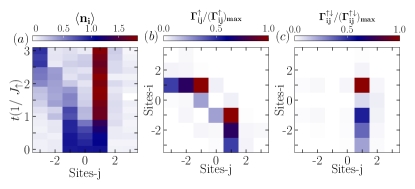
Figure 3: (a), (b) and (c) show the PS and ZNE error mitigated data of the time evolved density $\langle n_{i}\rangle$, correlation function $\Gamma_{ij}^{\uparrow}$ and $\Gamma_{ij}^{\uparrow\downarrow}$ respectively, for $U=V=10$ and $\delta=0.2$ obtained using the $ibmq\_brisbane$ hardware. The correlation functions are plotted at time $t=1.6(J^{-1})$ of the time evolution.

To further quantify the above observations, we plot the total particle density $\langle\hat{n}_{i}\rangle=\langle\hat{n}_{i,\uparrow}\rangle+\langle\hat{n}_{i,\downarrow}\rangle$ for each site as a function of time shown in Fig. 3(a), for fixed hopping imbalance $\delta=0.2$ and interaction strength $V=U=10$. The information about the doublon formation can be seen from the value $\langle n_{i}\rangle\sim 2$ at the $1^{st}$ site after a short time evolution and the independent dynamics of the $\uparrow$ particle on the left part of the central site as depicted in Fig. 3(a). Additionally, we also calculate the inter- and intra-component density density correlation

$$\Gamma_{ij}^{\uparrow\downarrow}(t)=\langle\hat{n}_{i,\uparrow}\hat{n}_{j,\downarrow}\rangle\ \ and\ \ \Gamma_{ij}^{\sigma}(t)=\langle\hat{a}_{i,\sigma}^{\dagger}\hat{a}_{j,\sigma}^{\dagger}\hat{a}_{j,\sigma}\hat{a}_{i,\sigma}\rangle$$ (6)

to identify the type of bound states present in the system. $\Gamma_{ij}^{\uparrow}$ and $\Gamma_{ij}^{\uparrow\downarrow}$ are plotted at time $t=1.6(J^{-1})$ in Fig. 3(b) and (c) respectively for same parameter values as in Fig. 3(a). The presence of a diagonal element in the $\Gamma_{ij}^{\uparrow\downarrow}$ as shown in Fig. 3(c) indicates the formation of an onsite doublon in the system. The weaker values of $\Gamma_{ij}^{\uparrow}$ immediately above or below the diagonal in Fig. 3(b) indicate the lesser probabilities of finding an NN pair ($\uparrow\uparrow$). For all the calculations in Fig. 2 and  3 we consider the parametrized circuit with eight layers of alternative single qubit $U_{3}$ and two-qubit control-Z gate. Note that for most parameter values considered here we find the fidelity $F(\Theta)$ is greater than $99\%$ and in fewer cases it is below $99\%$.

With this observation we confirm the dynamical creation of stable doublons in the QW of interacting fermions. Now it is essential to examine the stability of such a doublon in the dynamics which will be discussed in the following section.

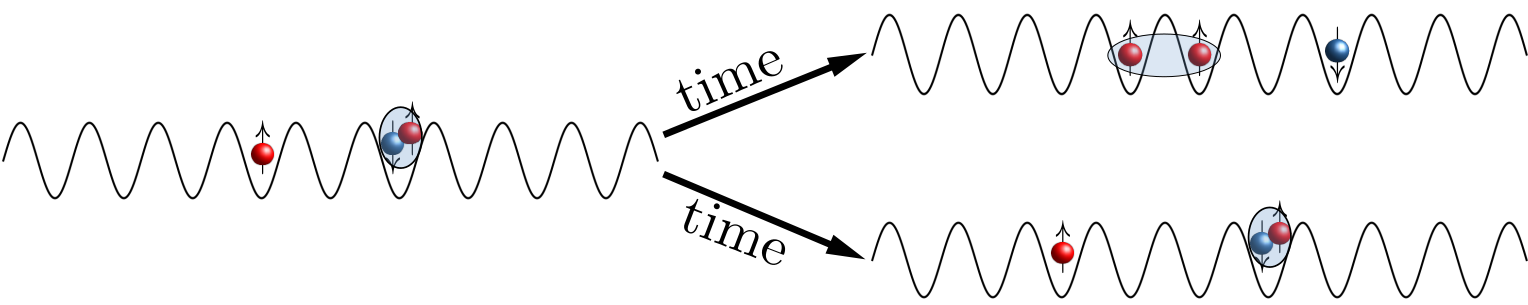
Figure 4: Shows two energy-conserving time evolution processes when we start from the initial state $|\psi(0)\rangle=\hat{a}_{-1,\uparrow}^{\dagger}\hat{a}_{1,\uparrow}^{\dagger}\hat{a}_{1,\downarrow}^{\dagger}|vac\rangle$.

Stability of doublon.- To examine the stability of the doublon we consider an initial state with one doublon and one $\uparrow$ particle at the right and left sites of the central site respectively. Such initial state is given as $|\psi(0)\rangle=\hat{a}_{-1,\uparrow}^{\dagger}\hat{a}_{1,\uparrow}^{\dagger}\hat{a}_{1,\downarrow}^{\dagger}|vac\rangle$ and is depicted in Fig. 4 (left). Naively, one would expect that for larger values of $\delta$, the onsite doublon will tend to dissociate completely and a stable NN pair ($\uparrow\uparrow$) will be formed as the latter one is energetically more stable. However, here we obtain a counter-intuitive situation. From the TEBD data shown in Fig. 5(a), we can see that $P_{\uparrow\downarrow}$ after some time saturates to finite values for different values of $\delta$ when $U=V=10$. As expected, for $\delta=0.2$, $P_{\uparrow\downarrow}$ saturates to a larger value close to one (red circles). For $\delta=1$, $P_{\uparrow\downarrow}$ saturates to a value close to $0.5$ (blue squares) due to the equal probability of the doublon and the NN pair ($\uparrow\uparrow$) states. However, when $\delta$ becomes larger than one, we obtain that $P_{\uparrow\downarrow}$ saturates to larger values compared to that for $\delta=1$ which is shown as black diamonds for $\delta=2$.

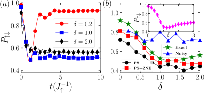
Figure 5: (a) Shows the TEBD data for $P_{\uparrow\downarrow}$ as a function of $t(J_{\uparrow}^{-1})$ for different values of $\delta$ when $U=V=10$ and $L=51$. (b) Shows the digital quantum simulation data for $P_{\uparrow\downarrow}$ plotted as a function of $\delta$ at time $t=2.5(J_{\uparrow}^{-1})$ for $U=V=10$. The green stars, bule triangles, black circles and red squares denote the exact, noisy, PS and PS+ZNE data respectively obtained using the $ibmq\_brisbane$ hardware. Inset shows $P_{\uparrow\downarrow}$ at time $t=10(J_{\uparrow}^{-1})$ as a function of $\delta$ obtained using TEBD for $U=V=10$ and $L=51$.

We also perform quantum computing implementation to observe the stability of the initially created doublon as a function of $\delta$. We plot the value of $P_{\uparrow\downarrow}$ at time $t=2.5(J_{\uparrow}^{-1})$ as a function of $\delta$ in Fig. 5(b) for $U=V=10$ where the data from the ED and quantum computing experiment show the initial decrease and then increase of $P_{\uparrow\downarrow}$ with increase in $\delta$. The inset of Fig. 5(b) shows the trend obtained from the TEBD simulations up to $\delta=3$ which confirms the results obtained from ED. The discrepancy between the ED and quantum computing experiment in Fig. 5(b) is due to the increase in noise with increase in circuit depth. Here we have considered a parametrized circuit of $12$ control-Z layers. For most of the parameter values we get the fidelity $F(\Theta)>97\%$ and in fewer cases we get lower fidelity than this.

This analysis shows that once the doublon is formed it remains stable at least up to 50 percent probability and never vanishes. Surprisingly, after reaching a minimum, the probability of stable doublon increases with increase in the hopping imbalance at the resonance condition i.e. $U=V$.

Conclusions.- In this work, we studied the QW of three interacting fermions in the context of an extended Fermi-Hubbard model and observed the signature of an onsite doublon formation using the quantum hardware. By implementing appropriate digital circuits for the model and utilizing the circuit optimization and various error mitigation techniques we obtained that the onsite doublons are spontaneously formed in the dynamics due to the combined effect of two competing interactions such as the inter-particle onsite interaction and the intra-particle NN interaction. The probability of doublon formation is found to be strongly dependent on the hopping imbalance between the constituents. Furthermore, we examined the stability of such doublons by analysing the QW from an initial state with already formed doublon and a free particle where we obtained that in any circumstances the probability of doublon survival is higher than the probability doublon dissociation.

Our work reveals two important results: (i) a route to form a stable doublon in the QW of non-local particles due to interaction. (ii) signature of such non-trivial doublon in a quantum computing experiments which was not observed in any other quantum simulators. This also opens up avenues and provides appropriate platform to explore dynamics of more interacting particles and the effect of perturbations such as disorder and tilt. One immediate extension can be the formation and stability of two or more doublons in the dynamics.

Acknowledgement.- We thank Sudhindu Bikash Mandal for useful discussions. T.M. acknowledges support from Science and Engineering Research Board (SERB), Govt. of India, through project No. MTR/2022/000382 and STR/2022/000023. T.M. also acknowledges MeitY QCAL project for providing access to use IonQ hardware through AWS Braket platform.

I Supplementary Material

I.1 Jordan-Wigner transformation

For the implementation of our operator on the quantum circuit we need to transform our Hamiltonian on spin-$\frac{1}{2}$ basis. We use the Jordan-Wigner transformation Somma et al. (2002) to map our Hamiltonian from Fock-space basis to spin-$\frac{1}{2}$ basis. The transformations of the operators are given as,

$$\hat{a}_{j,\uparrow}=\left(\prod_{i=0}^{j-1}\hat{\sigma}_{i}^{z}\right)\frac{\hat{\sigma}_{j}^{x}-i\hat{\sigma}_{j}^{y}}{2},\ \ \ \hat{n}_{j,\uparrow}=\frac{1}{2}(1-\hat{\sigma}_{j}^{z})$$

$$\hat{a}_{j,\downarrow}=\left(\prod_{i=L}^{L+j-1}\hat{\sigma}_{i}^{z}\right)\frac{\hat{\sigma}_{L+j}^{x}-i\hat{\sigma}_{L+j}^{y}}{2},\ \ \ \hat{n}_{j,\downarrow}=\frac{1}{2}(1-\hat{\sigma}_{L+j}^{z}),$$

where $\hat{\sigma}^{x},\hat{\sigma}^{y}$ and $\hat{\sigma}^{z}$ are the Pauli matrices. One can check that the transformation preserves anti-commutation relation i.e. $\{\hat{a}_{i,\sigma},\hat{a}_{j,\sigma}^{\dagger}\}=\delta_{ij}$, $\{\hat{a}_{i,\sigma}^{\dagger},\hat{a}_{j,\sigma}^{\dagger}\}=0$ and $\{\hat{a}_{i,\sigma},\hat{a}_{j,\sigma}\}=0$. We consider a one-dimensional system with $L$ lattice sites. As we are considering two different component systems we require $2L$ qubits to simulate our system. Here, we assign first $L$ qubits for $\uparrow$ component particles and remaining $L$ sites for the $\downarrow$ component particles.

With this, the transformed Hamiltonian corresponding to Eq. 1 is given as,

$$\hat{H}=\hat{H}_{0}+\hat{H}_{1}+\hat{H}_{2},$$ (7)

where,

$$\hat{H}_{0}=\sum_{j=0}^{L-2}\frac{J_{\uparrow}}{2}(\hat{\sigma}_{j}^{x}\hat{\sigma}_{j+1}^{x}+\hat{\sigma}_{j}^{y}\hat{\sigma}_{j+1}^{y})+\frac{V_{\uparrow\uparrow}}{4}\hat{\sigma}_{j}^{z}\hat{\sigma}_{j+1}^{z}$$

$$+\sum_{j=L}^{2L-2}\frac{J_{\downarrow}}{2}(\hat{\sigma}_{j}^{x}\hat{\sigma}_{j+1}^{x}+\hat{\sigma}_{j}^{y}\hat{\sigma}_{j+1}^{y})+\frac{V_{\downarrow\downarrow}}{4}\hat{\sigma}_{L+j}^{z}\hat{\sigma}_{L+j+1}^{z}$$

$$\hat{H}_{1}=\frac{U_{\uparrow\downarrow}}{4}\sum_{0}^{L-1}\hat{\sigma}_{j}^{z}\hat{\sigma}_{L+j}^{z}$$

$$\hat{H}_{2}=\sum_{j=1}^{L-2}(-\frac{V_{\uparrow\uparrow}}{2}\hat{\sigma}_{j}^{z}-\frac{V_{\downarrow\downarrow}}{2}\hat{\sigma}_{L+j}^{z})-\frac{V_{\uparrow\uparrow}}{4}(\hat{\sigma}_{0}^{z}+\hat{\sigma}_{L-1}^{z})$$

$$-\frac{V_{\downarrow\downarrow}}{4}(\hat{\sigma}_{L}^{z}+\hat{\sigma}_{2L-1}^{z})$$

Here we consider $V_{\uparrow\downarrow}=0$ as mentioned in the main text. We use this Hamiltonian (Eq. 7) to write the time evolution operator $\hat{U}$ of the main text. This unitary time evolution operator $\hat{U}$ can be converted into the quantum circuit and the details of which is given in the next section.

I.2 Time evolution on Quantum Circuit

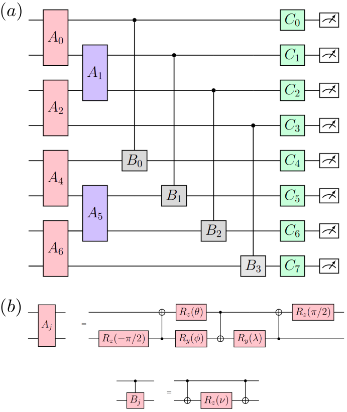
Figure 6: (a)Shows the circuit diagram for a single Trotter step. (b) Shows the explicit circuit diagram for the operators $A_{j}$ and $B_{j}$. Here we use $\theta=\frac{\pi}{2}-\frac{V_{\sigma\sigma}\Delta t}{2}$, $\phi=J_{\sigma}\Delta t-\frac{\pi}{2}$, $\lambda=\frac{\pi}{2}-J_{\sigma}\Delta t$ and $\nu=\frac{U_{\uparrow\downarrow}\Delta t}{2}$.

The first order Suzuki-Trotter decomposition of our time evolution operator $\hat{U}(t)$ for $n$ number of Trotter steps is given by,

$$\hat{U}(t) =e^{-i\hat{H}t}=\Big{(}e^{-i\hat{H}\Delta t}\Big{)}^{n}$$

$$=\Big{(}e^{-i\hat{H_{0}}\Delta t}e^{-i\hat{H_{1}}\Delta t}e^{-i\hat{H_{2}}\Delta t}\Big{)}^{n}+\mathcal{O}(n\Delta t^{2})$$

$$=\Big{(}\prod_{j=even}\hat{A}_{j}\prod_{i=odd}\hat{A}_{j}\prod_{j=0}^{L-1}\hat{B}_{j}\prod_{j=0}^{2L-1}\hat{C}_{j}\Big{)}^{n}+\mathcal{O}(n\Delta t^{2}).$$

To make the notation simpler we use,

$$\hat{A}_{j} =e^{-i\Delta t[J_{\sigma}/2(\hat{\sigma}_{j}^{x}\hat{\sigma}_{j+1}^{x}+\hat{\sigma}_{j}^{y}\hat{\sigma}_{j+1}^{y})+(V_{\sigma}/4)\hat{\sigma}_{j}^{z}\hat{\sigma}_{j+1}^{z}]},$$

$$\hat{B}_{j} =e^{-i\Delta t(U_{\uparrow\downarrow}/4)\hat{\sigma}_{j}^{z}\hat{\sigma}_{L+j}^{z}},$$

$$\hat{C}_{j} =e^{i\Phi_{j}\hat{\sigma}_{j}^{z}}$$

In the case of $\hat{A}_{j}$, $j$ can take values as $0\leq j\leq L-2$ and $L\leq j\leq 2L-2$, for $B_{j}$, $j$ runs from $0$ to $L-1$ and for $C_{j}$, $j$ can take values from $0$ to $2L-1$. Depending upon the sites $j$, the onsite rotation angles $\Phi_{j}$($\frac{V_{\uparrow\uparrow}\Delta t}{2}$ or $\frac{V_{\downarrow\downarrow}\Delta t}{2}$ or $\frac{V_{\uparrow\uparrow}\Delta t}{4}$ or $\frac{V_{\downarrow\downarrow}\Delta t}{4}$) changes. The Fig. 6(b) shows the quantum circuit for the expression $\hat{A}_{j}$ with the optimal number of gates Vatan and Williams (2004); Smith et al. (2019). The first-order Trotter circuit for a single Trotter step is shown in Fig. 6(a). The error depends on the time step $\Delta t$, which can be decreased by making the step size smaller. However, this will require more number Trotter steps which in turn increases the number of noisy quantum gates in the circuit. Therefore, we consider a moderately small $\Delta t=0.1$ in our calculation.

References

- Bloch et al. (2008) I. Bloch, J. Dalibard, and W. Zwerger, Rev. Mod. Phys. 80, 885 (2008).
- Moeckel and Kehrein (2010) M. Moeckel and S. Kehrein, New J. Phys. 12, 055016 (2010).
- Polkovnikov et al. (2011) A. Polkovnikov, K. Sengupta, A. Silva, and M. Vengalattore, Rev. Mod. Phys. 83, 863 (2011).
- Hubbard and Flowers (1963) J. Hubbard and B. H. Flowers, Proceedings of the Royal Society of London. Series A. Mathematical and Physical Sciences 276, 238 (1963).
- Yang (1989) C. N. Yang, Phys. Rev. Lett. 63, 2144 (1989).
- Winkler et al. (2006) K. Winkler, G. Thalhammer, F. Lang, R. Grimm, J. Hecker Denschlag, A. J. Daley, A. Kantian, H. P. Büchler, and P. Zoller, Nature 441, 853 (2006).
- Jördens et al. (2008) R. Jördens, N. Strohmaier, K. Günter, H. Moritz, and T. Esslinger, Nature 455, 204 (2008).
- Strohmaier et al. (2010) N. Strohmaier, D. Greif, R. Jördens, L. Tarruell, H. Moritz, T. Esslinger, R. Sensarma, D. Pekker, E. Altman, and E. Demler, Phys. Rev. Lett. 104, 080401 (2010).
- Greif et al. (2011) D. Greif, L. Tarruell, T. Uehlinger, R. Jördens, and T. Esslinger, Phys. Rev. Lett. 106, 145302 (2011).
- Meinert et al. (2013) F. Meinert, M. J. Mark, E. Kirilov, K. Lauber, P. Weinmann, A. J. Daley, and H.-C. Nägerl, Phys. Rev. Lett. 111, 053003 (2013).
- Jürgensen et al. (2014) O. Jürgensen, F. Meinert, M. J. Mark, H.-C. Nägerl, and D.-S. Lühmann, Phys. Rev. Lett. 113, 193003 (2014).
- Xia et al. (2015) L. Xia, L. A. Zundel, J. Carrasquilla, A. Reinhard, J. M. Wilson, M. Rigol, and D. S. Weiss, Nature Physics 11, 316 (2015).
- Covey et al. (2016) J. P. Covey, S. A. Moses, M. Gärttner, A. Safavi-Naini, M. T. Miecnikowski, Z. Fu, J. Schachenmayer, P. S. Julienne, A. M. Rey, D. S. Jin, and J. Ye, Nature Communications 7, 11279 (2016).
- de Hond et al. (2022) J. de Hond, J. Xiang, W. C. Chung, E. Cruz-Colón, W. Chen, W. C. Burton, C. J. Kennedy, and W. Ketterle, Phys. Rev. Lett. 128, 093401 (2022).
- Petrosyan et al. (2007) D. Petrosyan, B. Schmidt, J. R. Anglin, and M. Fleischhauer, Phys. Rev. A 76, 033606 (2007).
- Khomeriki et al. (2010) R. Khomeriki, D. O. Krimer, M. Haque, and S. Flach, Phys. Rev. A 81, 065601 (2010).
- Hofmann and Potthoff (2012) F. Hofmann and M. Potthoff, Phys. Rev. B 85, 205127 (2012).
- Kolovsky et al. (2012) A. R. Kolovsky, J. Link, and S. Wimberger, New Journal of Physics 14, 075002 (2012).
- Longhi and Della Valle (2012) S. Longhi and G. Della Valle, Phys. Rev. B 86, 075143 (2012).
- Santos and Dykman (2012) L. F. Santos and M. I. Dykman, New Journal of Physics 14, 095019 (2012).
- Chudnovskiy et al. (2012) A. L. Chudnovskiy, D. M. Gangardt, and A. Kamenev, Phys. Rev. Lett. 108, 085302 (2012).
- Longhi and Della Valle (2013) S. Longhi and G. Della Valle, Phys. Rev. A 87, 013634 (2013).
- Boschi et al. (2014) C. D. E. Boschi, E. Ercolessi, L. Ferrari, P. Naldesi, F. Ortolani, and L. Taddia, Phys. Rev. A 90, 043606 (2014).
- Wiater et al. (2017) D. Wiater, T. Sowiński, and J. Zakrzewski, Phys. Rev. A 96, 043629 (2017).
- Gärttner et al. (2019) M. Gärttner, A. Safavi-Naini, J. Schachenmayer, and A. M. Rey, Phys. Rev. A 100, 053607 (2019).
- Kempe (2003) J. Kempe, Contemporary Physics 44, 307–327 (2003).
- Venegas-Andraca (2012) S. E. Venegas-Andraca, Quantum Information Processing 11, 1015 (2012).
- Preiss et al. (2015) P. M. Preiss, R. Ma, M. E. Tai, A. Lukin, M. Rispoli, P. Zupancic, Y. Lahini, R. Islam, and M. Greiner, Science 347, 1229 (2015).
- Lahini et al. (2012) Y. Lahini, M. Verbin, S. D. Huber, Y. Bromberg, R. Pugatch, and Y. Silberberg, Phys. Rev. A 86, 011603 (2012).
- Giri et al. (2022) M. K. Giri, S. Mondal, B. P. Das, and T. Mishra, Phys. Rev. Lett. 129, 050601 (2022).
- Smith et al. (2019) A. Smith, M. S. Kim, F. Pollmann, and J. Knolle, npj Quantum Information 5, 106 (2019).
- Motta et al. (2020) M. Motta, C. Sun, A. T. K. Tan, M. J. O’Rourke, E. Ye, A. J. Minnich, F. G. S. L. Brandão, and G. K.-L. Chan, Nature Physics 16, 205 (2020).
- Vovrosh and Knolle (2021) J. Vovrosh and J. Knolle, Scientific Reports 11, 11577 (2021).
- Sun et al. (2021) S.-N. Sun, M. Motta, R. N. Tazhigulov, A. T. Tan, G. K.-L. Chan, and A. J. Minnich, PRX Quantum 2, 010317 (2021).
- Kamakari et al. (2022) H. Kamakari, S.-N. Sun, M. Motta, and A. J. Minnich, PRX Quantum 3, 010320 (2022).
- Chen et al. (2023) W. Chen, S. Zhang, J. Zhang, X. Su, Y. Lu, K. Zhang, M. Qiao, Y. Li, J.-N. Zhang, and K. Kim, npj Quantum Information 9, 122 (2023).
- Koh et al. (2023a) J. M. Koh, S.-N. Sun, M. Motta, and A. J. Minnich, Nature Physics 19, 1314 (2023a).
- Hoke et al. (2023) J. C. Hoke et al., Nature 622, 481 (2023).
- Shen et al. (2023) R. Shen, T. Chen, B. Yang, and C. H. Lee, (2023), arXiv:2311.10143 [quant-ph] .
- Azses et al. (2020) D. Azses, R. Haenel, Y. Naveh, R. Raussendorf, E. Sela, and E. G. Dalla Torre, Phys. Rev. Lett. 125, 120502 (2020).
- Smith et al. (2022) A. Smith, B. Jobst, A. G. Green, and F. Pollmann, Phys. Rev. Res. 4, L022020 (2022).
- Koh et al. (2022a) J. M. Koh, T. Tai, Y. H. Phee, W. E. Ng, and C. H. Lee, npj Quantum Information 8, 16 (2022a).
- Koh et al. (2022b) J. M. Koh, T. Tai, and C. H. Lee, Phys. Rev. Lett. 129, 140502 (2022b).
- Tan et al. (2023) A. T. K. Tan, S.-N. Sun, R. N. Tazhigulov, G. K.-L. Chan, and A. J. Minnich, Phys. Rev. A 107, 032614 (2023).
- Koh et al. (2023b) J. M. Koh, T. Tai, and C. H. Lee, (2023b), arXiv:2303.02179 [cond-mat.str-el] .
- Mei et al. (2020) F. Mei, Q. Guo, Y.-F. Yu, L. Xiao, S.-L. Zhu, and S. Jia, Phys. Rev. Lett. 125, 160503 (2020).
- Mi et al. (2022) X. Mi et al., Science 378, 785 (2022).
- Harle et al. (2023) N. Harle, O. Shtanko, and R. Movassagh, Nature Communications 14, 2286 (2023).
- Arute et al. (2020) F. Arute et al., (2020), arXiv:2010.07965 [quant-ph] .
- Anselme Martin et al. (2022) B. Anselme Martin, P. Simon, and M. J. Rančić, Phys. Rev. Res. 4, 023190 (2022).
- Stanisic et al. (2022) S. Stanisic, J. L. Bosse, F. M. Gambetta, R. A. Santos, W. Mruczkiewicz, T. E. O’Brien, E. Ostby, and A. Montanaro, Nature Communications 13, 5743 (2022).
- Wang et al. (2023) X. Wang, X. Feng, T. Hartung, K. Jansen, and P. Stornati, Phys. Rev. A 108, 022612 (2023).
- Rosenberg et al. (2023) E. Rosenberg et al., (2023), arXiv:2306.09333 [quant-ph] .
- Chen et al. (2022) I.-C. Chen, B. Burdick, Y. Yao, P. P. Orth, and T. Iadecola, Phys. Rev. Res. 4, 043027 (2022).
- Vidal (2003) G. Vidal, Phys. Rev. Lett. 91, 147902 (2003).
- Vidal (2004) G. Vidal, Phys. Rev. Lett. 93, 040502 (2004).
- Wall and Carr (2012) M. L. Wall and L. D. Carr, New J. Phys. 14, 125015 (2012).
- Jaschke et al. (2018) D. Jaschke, M. L. Wall, and L. D. Carr, Computer Physics Communications 225, 59 (2018).
- Fukuhara et al. (2013) T. Fukuhara, P. Schauß, M. Endres, S. Hild, M. Cheneau, I. Bloch, and C. Gross, Nature 502, 76 (2013).
- Li et al. (2020) W. Li, A. Dhar, X. Deng, K. Kasamatsu, L. Barbiero, and L. Santos, Phys. Rev. Lett. 124, 010404 (2020).
- Suzuki (1990) M. Suzuki, Physics Letters A 146, 319 (1990).
- Khatri et al. (2019) S. Khatri, R. LaRose, A. Poremba, L. Cincio, A. T. Sornborger, and P. J. Coles, Quantum 3, 140 (2019).
- Jones and Benjamin (2022) T. Jones and S. C. Benjamin, Quantum 6, 628 (2022).
- Heya et al. (2018) K. Heya, Y. Suzuki, Y. Nakamura, and K. Fujii, (2018), arXiv:1810.12745 [quant-ph] .
- Gray (2018) J. Gray, Journal of Open Source Software, 3(29), 819 (2018), 10.21105/joss.00819.
- McArdle et al. (2019) S. McArdle, X. Yuan, and S. Benjamin, Phys. Rev. Lett. 122, 180501 (2019).
- Li and Benjamin (2017) Y. Li and S. C. Benjamin, Phys. Rev. X 7, 021050 (2017).
- Temme et al. (2017) K. Temme, S. Bravyi, and J. M. Gambetta, Phys. Rev. Lett. 119, 180509 (2017).
- Kandala et al. (2019) A. Kandala, K. Temme, A. D. Córcoles, A. Mezzacapo, J. M. Chow, and J. M. Gambetta, Nature 567, 491 (2019).
- Somma et al. (2002) R. Somma, G. Ortiz, J. E. Gubernatis, E. Knill, and R. Laflamme, Phys. Rev. A 65, 042323 (2002).
- Vatan and Williams (2004) F. Vatan and C. Williams, Phys. Rev. A 69, 032315 (2004).