Evolving disorder and chaos induces acceleration of elastic waves

Abstract

Static or frozen disorder, characterised by spatial heterogeneities, influences diverse complex systems, encompassing many-body systems, equilibrium and nonequilibrium states of matter, intricate network topologies, biological systems, and wave-matter interactions. While static disorder has been thoroughly examined, delving into evolving disorder brings increased intricacy to the issue. An example of this complexity is the observation of stochastic acceleration of electromagnetic waves in evolving media, where noisy fluctuations in the propagation medium transfer effective momentum to the wave. Here, we investigate elastic wave propagation in a one-dimensional heterogeneous medium with diagonal disorder. We examine two types of complex elastic materials: one with static disorder, where mass density randomly varies in space, and the other with evolving disorder, featuring random variations in both space and time. Our results indicate that evolving disorder enhances the propagation speed of Gaussian pulses compared to static disorder. Additionally, we demonstrate that the acceleration effect also occurs when the medium evolves chaotically rather than randomly over time. The latter establishes that evolving randomness is not a unique prerequisite for observing wavefront acceleration, introducing the concept of chaotic acceleration in complex media.

I Introduction

A heterogeneous medium, characterised by spatial variations in physical properties, stands in contrast to homogeneous counterparts. These variations originate from localised changes in the medium’s properties and can be effectively modelled using continuous, piecewise, or random spatial functions Sahimi (2003); Bahraminasab et al. (2007). Found extensively in nature, materials exhibiting such inherent heterogeneity, including granular materials, porous media, glassy systems, the atmosphere, and colloidal suspensions, play crucial roles in technological and industrial applications influenced by human manipulation de Gennes (1999). Efforts to model complex materials have led to stochastic descriptions of processes within these systems Buryachenko (2007); Christakos (2012); Bahraminasab et al. (2007). These spatial random field models find applications in various real-world phenomena, such as transport processes in porous media Quintard and Whitaker (1993), oil reservoir characterisation parameters Sahimi (1992); Wu et al. (2006), and the spatial distribution of elastic moduli in polycrystals Hamanaka and Onuki (2006), granular materials Aoki and Ito (1996); Luding and Straub (2001); Trujillo et al. (2010), and composites Mohanty et al. (1982); Torquato (1985); Shalaev (1999). Numerical modelling has gained significant interest for practical applications, with acoustic and elastic wave propagation analysis serving as a key method for non-invasive tomography and seismic wave source characterisation in geophysics Boore (1972); Kelly et al. (1976); Frankel and Clayton (1984, 1986); Dablain (1986); Kneib and Kerner (1993).

Wave localisation, a robust phenomenon observed in various disordered systems with spatially dependent randomness, i.e. frozen disorder Lagendijk et al. (2009), has been a subject of significant exploration He and Maynard (1986); Maynard (2001); Sahimi et al. (2009). Phillip Anderson’s seminal work in 1958 demonstrated that frozen disorder can transform a conductor into an insulator, halting transport due to multiple scattering Anderson (1958). The exploration of waves in disordered media and localisation constitutes a highly intricate field, unveiling hitherto unknown phenomena such as Lévy flight Barthelemy et al. (2008) and hyper-transport Levi et al. (2012). Significantly, the dynamic evolution of disorder introduces nontrivial effects, as illustrated by Levi et al. Levi et al. (2012) in a paraxial optical context. Their findings revealed that an evolving random medium induces stochastic acceleration, facilitating the momentum exchange between the wave packet and the disorder. This process transcends diffusion, culminating in the attainment of ballistic transport Levi et al. (2012). The universality of this phenomenon extends its relevance to diverse wave systems featuring disorder.

Motivated by these observations, our investigation explores the propagation of elastic waves within a one-dimensional random medium featuring both frozen and evolving disorders in the mass-density distribution (diagonal disorder). Through extensive numerical simulations, we provide the first demonstration that evolving diagonal disorder induces stochastic acceleration of elastic waves. Our investigation considers two types of random fluctuations: one following a uniform distribution and another following a delta-correlated zero-mean Gaussian distribution. Additionally, we explore the effects of chaotic fluctuations in the mass-density of the propagating medium. We show that the system exhibits an equivalent acceleration of elastic waves under chaotic dynamics. Thus, evolving randomness is not a necessary condition for the acceleration of wavefronts in evolving media, an observation that leads us to coin the term chaotic acceleration in complex media. Moreover, we show that contrary to the case of stochastic acceleration, where acceleration is enhanced as the noise strength increases, there is a band of optimal levels of chaos where the system reaches an acceleration plateau. Thus, highly evolved chaos does not always give larger acceleration effects.

The remaining of the article is organised as follows. In Section II, we introduce our model for elastic wave propagation in one-dimensional heterogeneous materials with diagonal disorder. We also introduce here the models of disorder used for random frozen disorder, stochastic evolving disorder, and chaotic evolving disorder. In Section III, we show a summary of our results from numerical simulations. We first study in Section III.1 the effects of complexity through randomness (for frozen and evolving media), and in Section III.2 the effects of introducing complexity through chaos. Finally, we conclude and summarise our main results in Section IV.

II Elastic waves in heterogeneous media with diagonal disorder

II.1 The model

We will model a random heterogeneous medium that is, in some sense, close to a deterministic homogeneous reference medium Ostoja-Starzewski (2007). More abstractly, a random (complex) material is represented by a random medium $\mathcal{M}$ member of a family of random media $\mathcal{M}(\zeta)$, where $\zeta$ is a point in the space of events $\Lambda$ (sample space) Ostoja-Starzewski (2007); Gardiner (2009). In probability theory, $\Lambda$ consists of all possible outcomes $\zeta$ of an experiment or observation performed on a random system. The statistical description of the system is completed by providing a probability density function over the members of $\mathcal{M}(\zeta)$ Ostoja-Starzewski (2007); Gardiner (2009). The system’s physical properties are obtained through an ensemble average over multiple observations of the system so that the final results are statistically independent and could be related to experimental results. However, most heterogeneous materials are nonequilibrium, quenched disordered media for which no true statistical ensemble exists. Thus, our description of a heterogeneous system as a random medium corresponds to a heuristic model for the local random spatial variations of physical properties, limiting our study to simple models in which each member of the family $\mathcal{M}(\zeta)$ differs slightly from a homogeneous reference medium $\mathcal{M}^{0}$. In particular, we will consider random fluctuations introduced in the mass density $\rho$ of the medium, i.e.,

$$\rho(x,t)=\rho_{0}\left[1+\epsilon\eta(x,t)\right],$$ (1)

where $\eta(x,t)$ is a stochastic process which can also be random in space, $\rho_{0}$ is the mass density of the homogeneous reference medium, and $\epsilon$ is the noise strength. Here, we coined the term random frozen disorder for the case of a variable $\eta=\eta(x)$ that only depends on space. Alternatively, we shall use the term random evolving disorder for the case of a spatiotemporal variable $\eta=\eta(x,t)$. The random variable $\eta$ can take values from -1 to 1 and parameter $\epsilon$ can be regarded as a measure of the medium’s departure from homogeneity. Equation (1) describes what is known as diagonal disorder Ziman (1979) since it captures from a microscopic point of view fluctuations of a one-cite parameter: the mass of particles constituting the propagation medium.

Elastic waves propagating in a one-dimensional heterogeneous medium, whose linear mass-density $\rho$ varies randomly in space, are governed by the following hyperbolic wave equation,

$$\partial_{tt}\phi-c^{2}(x,t)\partial_{xx}\phi=0,$$ (2)

where $\phi$ is the dimensionless perturbation, and $c(x,t):=\sqrt{K_{0}/\rho(x,t)}$ is the phase velocity of waves. We assume that $K_{0}$ represents the bulk modulus of the homogeneous reference medium. In Appendix A, we provide a brief derivation of Eq. (2) from a microscopic model of elastic waves in a one-dimensional system with diagonal disorder. In the same spirit of the models studied in Refs. Bahraminasab et al. (2007); Shahbazi et al. (2005); Allaei and Sahimi (2006); Allaei et al. (2008), Eq. (2) can be regarded as a modified model based on elastic wave propagation in homogeneous media, where we have introduced spatial variations in the phase velocity to account for micro-structural density disorder Marín (2013); Alcântara et al. (2018); Discacciati et al. (2022, 2023).

II.2 Models of disorder

We consider three types of statistics for the disorder in this work:

• The first and most simple type corresponds to a random and uniform distribution of uncorrelated values for the variable $\eta$. We generate such noisy variable $\eta(x,t)$ in numerical simulations using standard algorithms for pseudo-random number generation at each space and time step.

• The second type of disorder assumes that statistical fluctuations of $\eta$ obey a Gaussian-type delta-correlated distribution in space with zero mean, i.e.,

  $$\langle\eta(x,t)\rangle=0,$$ (3a)

  $$C(x,t):=\left\langle\eta(x^{\prime},t^{\prime})\,\eta(x+x^{\prime},t+t^{\prime})\right\rangle_{x^{\prime},t^{\prime}}=\sigma^{2}\delta(x)\delta(t),$$ (3b)

  where $\sigma$, $\delta$, and $\langle\cdot\rangle$ denote the variance, the Dirac delta function, and the ensemble average with respect to the underlying Gaussian probability distribution, respectively. In our numerical simulations, we employed the Ziggurat method Marsaglia and Tsang (1984) to generate statistics of this kind. This method is widely employed in the literature to model various noisy sources in nature Gardiner (2009). Notice that from Eqs. (1) and (3) we have $\langle\rho\rangle=\rho_{0}$.

• We introduce a third type of evolving disorder modeled from a complex but deterministic source. In particular, at $t=0$, we considered a random distribution of uncorrelated values uniformly distributed in space for the field $\eta(x,t=0)$. Then, for each coordinate $x=x^{*}$, we introduced chaotic evolving disorder through time series generated from the well-known logistic map Strogatz (2018) ,

  $$\eta_{n+1}(x^{*})=r\eta_{n}(x^{*})\left[1-\eta_{n}(x^{*})\right],$$ (4)

  famously known for exhibiting intermittency and a period-doubling route to chaos as the bifurcation parameter $r$ increases within the interval $[0,4]$. Evolving chaos is obtained for $r>r_{c}\simeq 3.56995$, except for the isolated ranges corresponding to the periodic windows of the logistic map. One obtains completely developed chaos for $r=4$.

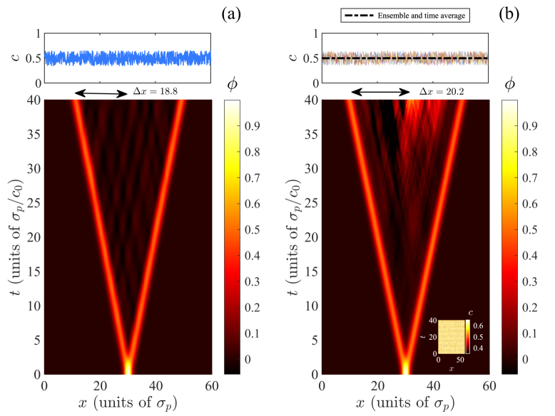
Figure 1: Typical behaviour of waves in random complex media with an underlying uniform probability distribution. Cases are shown for a single disorder realisation with disorder strength $\epsilon=0.3$. The colour scale indicates the field of the elastic wave $\phi$. (a) Evolution under frozen randomness. The upper panel shows the random fluctuations of the phase velocity $c$ in space for a single realisation. (b) Evolution under evolving randomness. The inset shows a realisation of the random disorder in the phase speed. The upper panel shows the random fluctuations of the phase velocity $c$ in space at $t=0$ for various disorder realisations, along with the time and ensemble-averaged speed over 500 realisations (black dashed-dotted line).

III Results

We simulate numerically the time evolution of an initially-at-rest Gaussian wave packet of width $\sigma_{p}$, given by

$$\phi(x,t=0)=\exp\left(-\frac{(x-x_{0})^{2}}{2\sigma_{p}^{2}}\right),$$ (5)

governed by Eq. (2) considering free-end (Neumann) boundary conditions. Hereon, we shall consider only dimensionless variables where the space $x$ is measured in units of $\sigma_{p}$, and time $t$ is measured in units of $\sigma_{p}/c_{0}$, where $c_{0}=\sqrt{K_{0}/\rho_{0}}$ is the phase speed of elastic waves in the homogeneous reference medium. At $t=0$, the wavepacket is stationary and centred at $x_{0}=L/2$ (the centre of the space domain), with $L=60$. We used 800 discrete nodes in space and finite differences of second-order accuracy for the space derivatives with step $\Delta x=0.075$. For the time integration, we used the Dormand-Prince algorithm as an explicit Runge-Kutta of orders 4 and 5 with an adaptive time step Shampine and Reichelt (1997). We calculated 500 statistical realisations of the disorder for each combination of parameters using a parallel code written in Matlab ©, and we have verified that the ensemble average of the speed and the amplitude fields becomes statistically invariant.

III.1 Complexity through randomness: frozen and evolving media

Figure 1 shows typical instances of wave propagation in a random media obtained under frozen randomness [Fig. 1(a)] and evolving randomness [Fig. 1(b)]. We considered uniform probability density distributions with $\epsilon=0.3$ in both cases. In the trivial homogeneous case where the phase speed $c$ is constant, it is well known that under Eq. (2), an initially at-rest Gaussian wavepacket breaks into two counterpropagating pulses with half the amplitude of the initial pulse. In Figure 1(a), the initially at-rest Gaussian wavepacket also breaks into two counterpropagating pulses in our heterogeneous material. These two pulses propagate at nearly constant speed, and multiple backscattering due to the spatial disorder within the density of the medium produces a small amplitude interference pattern observed in the region between them. The upper panel in Fig. 1(a) shows a typical statistical realisation of the frozen disorder induced in the phase speed in the heterogeneous medium, which is indeed random in space with mean value $c_{0}=0.5$.

For the case of evolving randomness, Fig. 1(b) shows that the multiple backscattering produces a larger amplitude interference pattern than the case of frozen randomness. These patterns are also more complex and emerge from the spatiotemporal complexity of the phase velocity (see inset in Fig. 1(b)). The upper panel in Fig. 1(b) shows several statistical realisations of the phase velocity at $t=0$. The ensemble average of the phase speed after 500 disorder realisations gives an almost constant phase speed $\langle c\rangle=c_{0}=0.5$, as shown with a black dashed-dotted line in the upper panel of Fig. 1(b). We have noticed that the counterpropagating pulses travel faster under random evolving disorder than under random frozen disorder. As indicated with double arrows in Fig. 1, during the same time interval $\Delta t=40$, the pulse travels a distance $\Delta x\simeq 18.8$ under random frozen disorder and $\Delta x\simeq 20.2$ under random evolving disorder. This observation suggests an acceleration process occurs in the evolving medium compared to the frozen case. To inquire about this observation, we computed the ensemble average of the pulse speed for different values of $\epsilon$ and compared the observed behaviour between frozen and evolving cases. Figure 2(a) reveals that as the strength of frozen randomness increases, the speed of travelling pulses decreases, and thus the wave tends to localise. Indeed, spatial randomness is expected to induce a strong tendency for waves to localise in one-dimensional systems. Surprisingly, Fig. 2(a) also reveals that the speed slightly increases as the strength of the evolving randomness increases. Thus, increasing the disorder strength in evolving media, rather than promoting wave localisation, enhances wave transport. Consequently, for a fixed value of $\epsilon$, waves travel faster under a random evolving disorder than under a random frozen disorder.

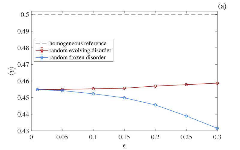
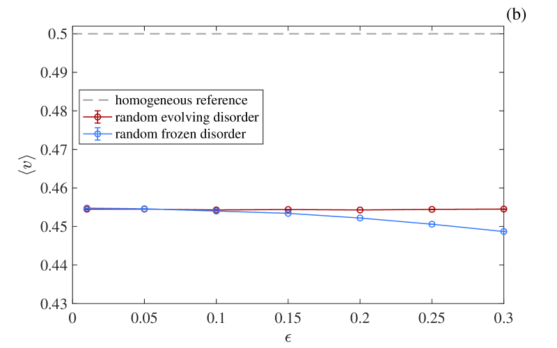
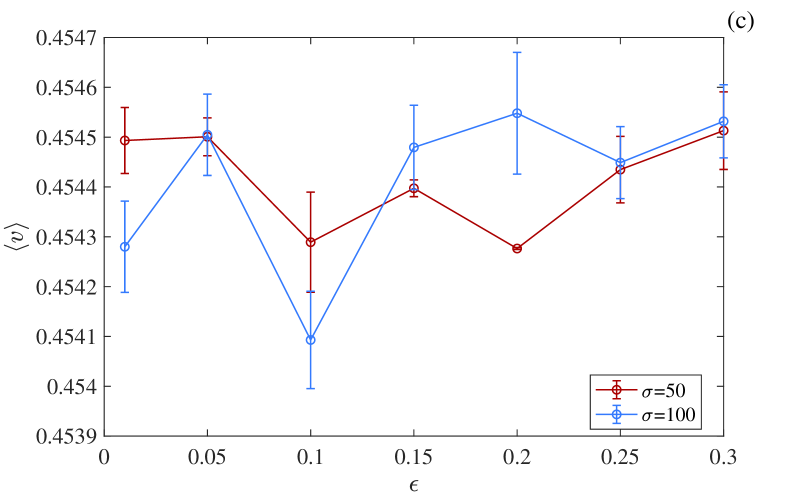
Figure 2: Stochastic-induced acceleration of elastic waves: Ensemble average speed $\langle v\rangle$ as a function of disorder strength $\epsilon$ for (a) uniform distribution, and (b) delta-correlated normal distribution with zero mean and variance $\sigma=50$. Error bars are too small to be shown in the scale. (c) Dependence of the ensemble average speed as a function of the variance of the underlying normal distribution. The speed of the wave under evolving randomness remains almost invariant under changes in the variance and noise strength.

Thus, we have discovered a kind of stochastic-induced acceleration in the propagation of elastic waves. This phenomenon is very similar to that observed by Levi et al. in Ref. Levi et al. (2012), where hyper-transport of light by evolving disorder is reported numerically and experimentally using an effective 2+1-dimensional paraxial optical setting. Here, we report a similar phenomenon for elastic waves in an evolving 1+1-dimensional randomly disordered medium.

We determined that the observed phenomenon is robust against changes in the underlying probability distributions. In Fig. 2(b), we considered a delta-correlated normal distribution with $\sigma=50$, following Eq. (3), and obtained the same qualitative behaviour. In this case, random frozen disorder enhances a weaker localisation than the case of frozen uniform randomness [see Fig. 2(a)]. This is because samples of a random variable under a Gaussian probability distribution predominantly accumulate near its mean value, and extreme events corresponding to the tails of the Gaussian distribution are less probable to occur. This frozen randomness with accumulated values near the mean induces a weaker wave localisation in contrast with a uniform distribution, where samples away from the mean are equally probable to occur than values near the mean. Similarly, evolving randomness following a Gaussian distribution leads to a weaker enhancement of wave transport when compared to the case of uniform distributions. However, as evidenced in Fig. 2(b), the evolving randomness counteracts wave localisation, sustaining the speed at a nearly constant value as the disorder strength increases.

Following the previous observations, it is natural to wonder about the effect of a Gaussian probability distribution with a higher dispersion of sample points. Thus, we repeated our analysis with a variance $\sigma=100$, i.e. twice as that in Fig. 2(b). Figure 2(c) shows minimal differences in the outcome from the ensemble average speed. Thus, although extreme events are more probable for $\sigma=100$ than for $\sigma=50$, they are still much less probable than events near the mean of the stochastic process. Thus, the effect of enhanced transport under evolving randomness is qualitatively the same for both variance values.

III.2 Complexity through chaos: chaotic acceleration in complex media

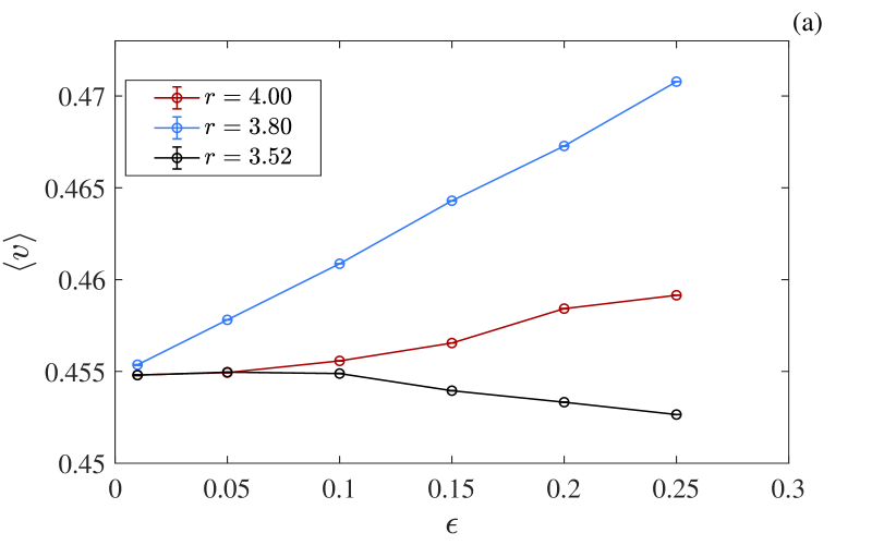
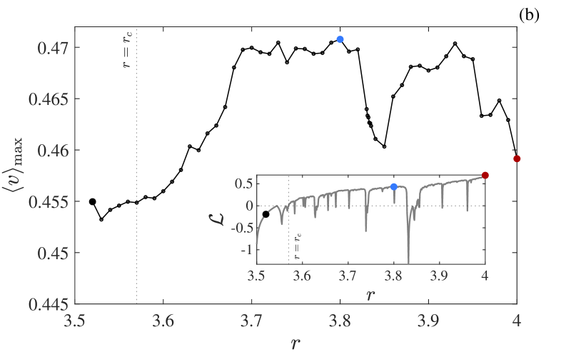
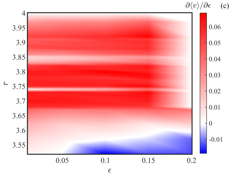
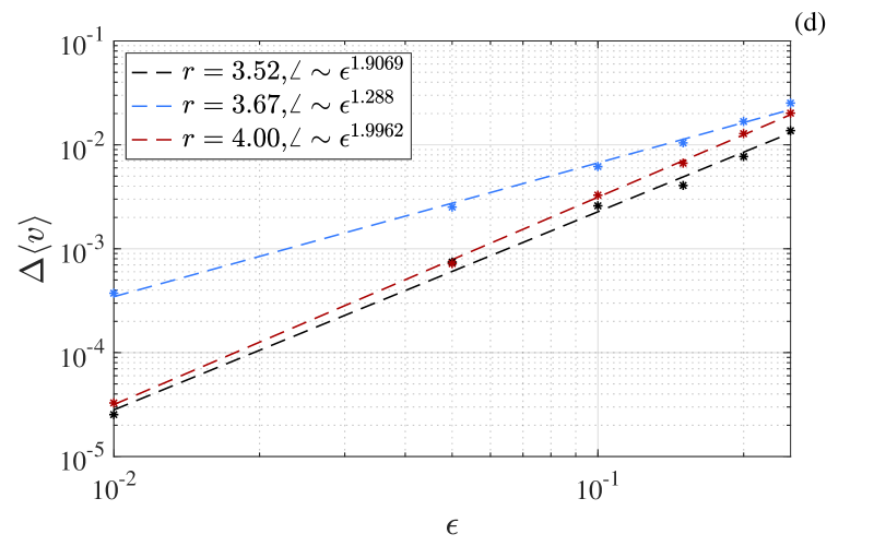
Figure 3: Chaos-induced acceleration of elastic waves: (a) Ensemble average speed $\langle v\rangle$ as a function of disorder strength $\epsilon$ for different values of the bifurcation parameter $r$. (b) Maximum speed of elastic waves as a function of the bifurcation parameter. The maximum values are obtained within a broad bandwidth of $r$. The inset shows the Lyapunov exponent $\mathcal{L}$ as a function of $r$ along with three sample points used to characterise the speed dependence on the chaos level (black, blue and red dots). (c) Phase space representation, indicating regions in the parameter space $(\epsilon,r)$ where localisation (blue regions) and chaos-induced acceleration (red regions) are observed. (d) Measured scaling laws of the chaos-induced acceleration with the disorder strength. Error bars are too small to be shown in the scale.

Following our previous observations, we wondered if the evolving nature of the media must be strictly random to induce the acceleration of elastic waves. Thus, we explored the outcome of the system if the medium evolves in a deterministic but complex way, following the logistic map shown in Eq. (4). We have discovered that chaos also induces the same qualitative acceleration effect, as summarised in Fig. 3. Our explorations lead us to coin the term chaotic acceleration in complex media.

In Fig. 3(a), we show the ensemble-averaged speed of elastic waves as a function of the disorder strength $\epsilon$ for different bifurcation parameter $r$ values. For $r=3.52$, the logistic map exhibits a periodic orbit with period $4$. We observe that the wave tends to localise as $\epsilon$ increases. In this case, the elastic waves undergo multiple scattering at localised heterogeneities periodically modulated in time. Thus, the wave tends to localise as the amplitude of such modulations becomes larger.

However, we notice that for $r=3.80$, a value of the bifurcation parameter where the system evolves chaotically, there is a remarkable increase of the wave speed as the disorder strength $\epsilon$ increases, as shown in Fig. 3(a). Indeed, $\langle v\rangle$ increases monotonically with $\epsilon$. Importantly, comparing Fig. 2(a) and Fig. 2(b) with Fig. 3(a), we notice that chaotic dynamics in the evolving medium induces a larger increase of the wave speed than in the stochastic case.

We have systematically studied the ensemble-averaged speed of waves for increasing bifurcation parameter values. For $r=4$, the value at which the medium exhibits completely evolved chaos, one might expect that the effect of increased transport will reach its stronger regime. However, we have found that the accelerating effect is more moderate than for $r=3.80$, as shown in Fig. 3(a). The latter evidences an optimal value of $r$ (and thus, an optimal level of chaos), where the chaotically induced transport is stronger.

We have computed the maximum value of $\langle v\rangle_{\max}$ in terms of the bifurcation parameter $r$ in Fig. 3(b). We observe that the maximum ensemble-averaged speed reaches a maximum plateau for intermediate values of $r$ within the interval $[r_{c},\,4]$, where $r_{c}\simeq 3.56995$ is the critical value for the onset of chaos in the logistic map. A black point in Fig. 3(b) indicates the case $r=3.52$, which corresponds to the non-chaotic dynamics of the system. The blue point in Fig. 3(b) indicates the case where we have detected the largest value of $\langle v\rangle$, corresponding to $r=3.80$. The red point Fig. 3(b) corresponds to the case of completely evolved chaos for $r=4$.

Notice in Fig. 3(b) that there are ranges for the breakdown of the chaotic acceleration effect in the middle of the chaotic acceleration plateau. These breakdown ranges of $r$ correspond to sub-ranges of $[r_{c},\,4]$ where the speed decays abruptly due to the emergence of the periodic windows of the logistic map. Indeed, in the inset of Fig. 3(b), we show the Lyapunov exponent $\mathcal{L}$ of the logistic map, evidencing that the broadest range of acceleration breakdown corresponds to the wider periodic window of the logistic map. For each periodic window of the logistic map, which is fractally distributed within the range $[r_{c},\,4]$, there will be a corresponding breakdown of the chaotic acceleration effect. Also, in the inset of Fig. 3(b), we show the cases corresponding to $r=3.52$, $r=3.80$ and $r=4$, with black, blue and red dots, respectively, to emphasise that highly evolved chaos do not imply higher acceleration effects: an optimum value is somewhere in between the points $r=r_{c}$ and $r=4$.

Figure 3(c) shows a diagram in the parameter space $(\epsilon,r)$ of the chaotic system. Here, the colour scale indicates the value of $\partial\langle v\rangle/\partial\epsilon$. Thus, red regions indicate combinations of parameters for chaotic acceleration, whereas white and blue regions are for localisation. Notice that the breakdowns of chaotic acceleration emerge as white stripes within red regions in parameter space.

Finally, in Fig. 3(d), we study the scaling laws of the ensemble-averaged speed jumps, $\Delta\langle v\rangle$, with the disorder strength $\epsilon$. We observe that, although $\langle v\rangle$ can reach large values for $r=3.67$ than for $r=4$, it grows faster with $\epsilon$ for completely evolved chaos ($r=4$) than for moderate chaos ($r=3.67$). Indeed, it is clear that $\partial\langle v\rangle/\partial\epsilon\sim\epsilon^{1.288}$ for $r=3.67$, and $\partial\langle v\rangle/\partial\epsilon\sim\epsilon^{1.9962}$ for $r=4$. Thus, although the largest ensemble-averaged speed occurs for moderate chaos, the ensemble-averaged speed increases faster with $\epsilon$ for completely evolved chaos.

IV Conclusions

In summary, we have shown that evolving disorder, random or chaotic, enhances the acceleration of elastic waves in one-dimensional systems under diagonal disorder. Using as a model a hyperbolic partial differential equation with space-time variations in the phase velocity, we have characterised the acceleration effect considering three types of statistics for the disorder: uniform (random), Gaussian (random), and chaotic (deterministic) distributions. Under frozen disorder, elastic waves localise as the disorder strength increases. However, we have shown that evolving random disorder tends to increase the speed of wavefronts as the disorder’s strength increases. We have discussed similarities between the observed phenomenon and the hyper-transport of light observed by other researchers in random evolving media Levi et al. (2012). Furthermore, we have discovered that chaotic (deterministic) evolving disorder induces the same acceleration effect. Thus, randomness is not a unique prerequisite to observing enhanced transport. We have characterised the chaotic acceleration effect considering chaotic signals generated from a logistic map and show that the maximum value of the ensemble-averaged speed reaches a maximum plateau within an interval of the bifurcation parameter of the logistic map. We provide evidence of the breakdown of chaotic acceleration at intervals of the bifurcation parameter corresponding to the periodic windows of the logistic map, thus supporting the hypothesis that acceleration in such deterministic systems is purely enhanced by chaos and not by periodic signals composed of a large number of frequencies.

Appendix A Derivation of the wave equation under diagonal disorder

Elastic wave propagation in a one-dimensional medium can be described microscopically by a system of $n$ consecutive point-like particles of mass $m_{j}$ coupled by springs with a Hooke’s constant $k_{j}$ ($j=1,\ldots,n-1$). Diagonal disorder corresponds to the situation where $k_{j}=k$ is constant and deterministic, whereas $m_{j}$ for $j=1,\ldots,n$ is given by a stochastic process. Let $\phi_{j}(\omega,t)$ be the displacement from equilibrium of particle $j$ at time $t$ in a realisation $\omega(t)$ of the random evolving medium. If such displacements are small compared to the inter-particle distance $a$, the system exhibits a linear response to external perturbations and the stochastic equation of motion for the $j$-th mass within the bulk of the material ($j=2,\dots,n-1$) reads

$$a\rho_{j}(\omega,t)\frac{d^{2}\phi_{j}}{dt^{2}}=-\frac{2K_{0}}{a}\phi_{j}+\frac{K_{0}}{a}(\phi_{j+1}+\phi_{j-1}),$$ (6)

where $\rho_{j}(\omega,t):=m_{j}(\omega(t))/a$ and $K_{0}:=ak$ are the microscopic mass density and stiffness of the medium, respectively. We can use some coarse-graining strategy to obtain a continuous (macroscopic) wave equation from Eq. (6). The use of integral representations through weighted space-time averages of particle quantities is one such alternative Murdoch (2012), which can be achieved by multiplying both sides of Eq. (6) by a smoothing kernel of radius $h$, namely $f(x-x_{j},h)$, and integrating over $x_{j}$ Murdoch and Bedeaux (1994); Glasser and Goldhirsch (2001); Goldhirsch and Goldenberg (2002). This type of coarse-graining formalism is known to solve problems related to discontinuities and the lack of derivatives in many stochastic processes, such as the case of fractional Brownian motions (as shown in Mandelbrot’s seminal work on Ref. Mandelbrot and Ness (1968)). Here, we assume that the kernel $f$ has a compact support domain $\mathcal{S}(x)$ of radius $h$ around $x_{j}$, i.e. the function $f$ vanishes if $|x-x_{j}|\geq h$ Marín et al. (2014); Petit et al. (2014). Thus, the left-hand side of Eq. (6) becomes

$$a\int_{\mathcal{S}(x)}\rho_{j}(\omega,t)\frac{d^{2}\phi_{j}}{dt^{2}}f(x-x_{j},h)dx_{j}=a\langle\rho(x,t)\partial_{tt}\phi(x,t)\rangle_{h},$$ (7)

where $\langle\cdot\rangle_{h}$ denotes the continuum function obtained after coarse-graining with a smoothing function of radius $h$. Similarly, the right-hand side of Eq. (6) after coarse-graining and using a Taylor expansion for $\phi_{j\pm 1}-\phi_{j}\gg a\forall j$, becomes

$$\frac{K_{0}}{a}\int_{\mathcal{S}(x)}(\phi_{j+1}-2\phi_{j}-\phi_{j-1})f(x-x_{j},h)dx_{j}=aK_{0}\langle\partial_{xx}\phi(x,t)\rangle_{h}.$$ (8)

Equating Eqs. (7) and (8), setting $c(x,t):=\sqrt{K_{0}/\rho(x,t)}$, we obtain a hyperbolic partial differential equation of the same form as Eq. (2).

References

- Sahimi (2003) M. Sahimi, “Heterogeneous materials, volume I: Morphology, and linear transport and optical properties,” (Springer-Verlag, New York, 2003).
- Bahraminasab et al. (2007) Alireza Bahraminasab, S Mehdi Vaez Allaei, Farhad Shahbazi, Muhammad Sahimi, MD Niry, and M Reza Rahimi Tabar, “Renormalization group analysis and numerical simulation of propagation and localization of acoustic waves in heterogeneous media,” Physical Review B 75, 064301 (2007).
- de Gennes (1999) P. G. de Gennes, “Granular matter: a tentative view,” Rev. Mod. Phys. 71, S374–S382 (1999).
- Buryachenko (2007) Valeriy Buryachenko, Micromechanics of heterogeneous materials (Springer Science & Business Media, 2007).
- Christakos (2012) George Christakos, Random field models in earth sciences (Courier Corporation, 2012).
- Quintard and Whitaker (1993) Michel Quintard and Stephen Whitaker, “Transport in ordered and disordered porous media: volume-averaged equations, closure problems, and comparison with experiment,” Chemical Engineering Science 48, 2537–2564 (1993).
- Sahimi (1992) Muhammad Sahimi, “Brittle fracture in disordered media: from reservoir rocks to composite solids,” Physica A: Statistical Mechanics and its Applications 186, 160–182 (1992).
- Wu et al. (2006) Kejian Wu, Marinus IJ Van Dijke, Gary D Couples, Zeyun Jiang, Jingsheng Ma, Kenneth S Sorbie, John Crawford, Iain Young, and Xiaoxian Zhang, “3D stochastic modelling of heterogeneous porous media–applications to reservoir rocks,” Transport in porous media 65, 443–467 (2006).
- Hamanaka and Onuki (2006) Toshiyuki Hamanaka and Akira Onuki, “Transitions among crystal, glass, and liquid in a binary mixture with changing particle-size ratio and temperature,” Physical Review E 74, 011506 (2006).
- Aoki and Ito (1996) Keiko M. Aoki and Nobuyasu Ito, “Effect of size polydispersity on granular materials,” Physical Review E 54, 1990–1996 (1996).
- Luding and Straub (2001) S. Luding and O. Straub, “The equation of state of polydisperse granular gases — Granular gases. Eds. T. Pöschel and S. Luding.” (Springer, Berlin, 2001) p. 389.
- Trujillo et al. (2010) Leonardo Trujillo, Franklin Peniche, and Leonardo Di G Sigalotti, “Derivation of a Schrödinger-like equation for elastic waves in granular media,” Granular Matter 12, 417–436 (2010).
- Mohanty et al. (1982) KK Mohanty, JM Ottino, and HT Davis, “Reaction and transport in disordered composite media: introduction of percolation concepts,” Chemical Engineering Science 37, 905–924 (1982).
- Torquato (1985) S Torquato, “Effective electrical conductivity of two-phase disordered composite media,” Journal of Applied Physics 58, 3790–3797 (1985).
- Shalaev (1999) Vladimir M Shalaev, Nonlinear optics of random media: fractal composites and metal-dielectric films, Vol. 158 (Springer Science & Business Media, 1999).
- Boore (1972) David M Boore, “Finite difference methods for seismic wave propagation in heterogeneous materials,” in Methods in computational physics, Vol. 11, edited by Fernbach and M. Rotenberg (Academic Press New York, 1972) pp. 1–37.
- Kelly et al. (1976) Kenneth R Kelly, Ronald W Ward, Sven Treitel, and Richard M Alford, “Synthetic seismograms: A finite-difference approach,” Geophysics 41, 2–27 (1976).
- Frankel and Clayton (1984) Arthur Frankel and Robert W Clayton, “A finite-difference simulation of wave propagation in two-dimensional random media,” Bulletin of the Seismological Society of America 74, 2167–2186 (1984).
- Frankel and Clayton (1986) Arthur Frankel and Robert W Clayton, “Finite difference simulations of seismic scattering: Implications for the propagation of short-period seismic waves in the crust and models of crustal heterogeneity,” Journal of Geophysical Research: Solid Earth 91, 6465–6489 (1986).
- Dablain (1986) MA Dablain, “The application of high-order differencing to the scalar wave equation,” Geophysics 51, 54–66 (1986).
- Kneib and Kerner (1993) Guido Kneib and Claudia Kerner, “Accurate and efficient seismic modeling in random media,” Geophysics 58, 576–588 (1993).
- Lagendijk et al. (2009) Ad Lagendijk, Bart van Tiggelen, and Diederik S. Wiersma, “Fifty years of Anderson localization,” Physics Today 62, 24–29 (2009).
- He and Maynard (1986) Shanjin He and JD Maynard, “Detailed measurements of inelastic scattering in Anderson localization,” Physical review letters 57, 3171 (1986).
- Maynard (2001) Julian D Maynard, “Acoustical analogs of condensed-matter problems,” Reviews of modern physics 73, 401 (2001).
- Sahimi et al. (2009) Muhammad Sahimi, M Reza Rahimi Tabar, Alireza Bahraminasab, Reza Sepehrinia, and SM Vaez Allaei, “Propagation and localization of acoustic and elastic waves in heterogeneous materials: renormalization group analysis and numerical simulations,” Acta mechanica 205, 197–222 (2009).
- Anderson (1958) Philip W Anderson, “Absence of diffusion in certain random lattices,” Physical Review 109, 1492 (1958).
- Barthelemy et al. (2008) Pierre Barthelemy, Jacopo Bertolotti, and Diederik S Wiersma, “A Lévy flight for light,” Nature 453, 495–498 (2008).
- Levi et al. (2012) Liad Levi, Yevgeny Krivolapov, Shmuel Fishman, and Mordechai Segev, “Hyper-transport of light and stochastic acceleration by evolving disorder,” Nature Physics 8, 912–917 (2012).
- Ostoja-Starzewski (2007) Martin Ostoja-Starzewski, Microstructural randomness and scaling in mechanics of materials (CRC Press, 2007).
- Gardiner (2009) Crispin Gardiner, Stochastic methods, Vol. 4 (Springer Berlin, 2009).
- Ziman (1979) John M Ziman, Models of disorder: the theoretical physics of homogeneously disordered systems (Cambridge university press, 1979).
- Shahbazi et al. (2005) F. Shahbazi, Alireza Bahraminasab, S. Mehdi Vaez Allaei, Muhammad Sahimi, and M. Reza Rahimi Tabar, “Localization of elastic waves in heterogeneous media with off-diagonal disorder and long-range correlations,” Phys. Rev. Lett. 94, 165505 (2005).
- Allaei and Sahimi (2006) S. Mehdi Vaez Allaei and Muhammad Sahimi, “Shape of a wave front in a heterogenous medium,” Phys. Rev. Lett. 96, 075507 (2006).
- Allaei et al. (2008) SM Vaez Allaei, Muhammad Sahimi, and M Reza Rahimi Tabar, “Propagation of acoustic waves as a probe for distinguishing heterogeneous media with short-range and long-range correlations,” Journal of Statistical Mechanics: Theory and Experiment 2008, P03016 (2008).
- Marín (2013) Juan F Marín, Modelado computacional de la propagación de ondas en medios heterogéneos, Tech. Rep. (Undergraduate thesis, Universidad Central de Venezuela, 2013).
- Alcântara et al. (2018) Adriano A Alcântara, Haroldo R Clark, and Mauro A Rincon, “Theoretical analysis and numerical simulation for a hyperbolic equation with Dirichlet and acoustic boundary conditions,” Computational and Applied Mathematics 37, 4772–4792 (2018).
- Discacciati et al. (2022) Marco Discacciati, Claudia Garetto, and Costas Loizou, “Inhomogeneous wave equation with t-dependent singular coefficients,” Journal of Differential Equations 319, 131–185 (2022).
- Discacciati et al. (2023) Marco Discacciati, Claudia Garetto, and Costas Loizou, “On the wave equation with space dependent coefficients: Singularities and lower order terms,” Acta Applicandae Mathematicae 187, 10 (2023).
- Marsaglia and Tsang (1984) George Marsaglia and Wai Wan Tsang, “A fast, easily implemented method for sampling from decreasing or symmetric unimodal density functions,” SIAM Journal on scientific and statistical computing 5, 349–359 (1984).
- Strogatz (2018) Steven H Strogatz, Nonlinear dynamics and chaos: With applications to physics, biology, chemistry, and engineering (CRC press, 2018).
- Shampine and Reichelt (1997) Lawrence F. Shampine and Mark W. Reichelt, “The MATLAB ODE suite,” SIAM Journal on Scientific Computing 18, 1–22 (1997).
- Murdoch (2012) A Ian Murdoch, Physical foundations of continuum mechanics (Cambridge University Press, 2012).
- Murdoch and Bedeaux (1994) A. I. Murdoch and D. Bedeaux, “Continuum equations of balance via weighted averages of microscopic quantities,” Proceedings of the Royal Society of London. Series A: Mathematical and Physical Sciences 445, 157–179 (1994).
- Glasser and Goldhirsch (2001) B. J. Glasser and I. Goldhirsch, “Scale dependence, correlations, and fluctuations of stresses in rapid granular flows,” Physics of Fluids 13, 407–420 (2001).
- Goldhirsch and Goldenberg (2002) I Goldhirsch and C Goldenberg, “On the microscopic foundations of elasticity,” The European Physical Journal E 9, 245–251 (2002).
- Mandelbrot and Ness (1968) Benoit B. Mandelbrot and John W. Van Ness, “Fractional Brownian motions, fractional noises and applications,” SIAM Review 10, 422–437 (1968).
- Marín et al. (2014) Juan F. Marín, Juan C. Petit, Leonardo Di. G. Sigalotti, and Leonardo Trujillo, “Integral representation for continuous matter fields in granular dynamics,” in Computational and Experimental Fluid Mechanics with Applications to Physics, Engineering and the Environment, edited by Leonardo Di G. Sigalotti, Jaime Klapp, and Eloy Sira (Springer International Publishing, Cham, 2014) pp. 473–480.
- Petit et al. (2014) Juan C. Petit, Juan F. Marín, and Leonardo Trujillo, “On the construction of a continuous theory for granular flows,” in Computational and Experimental Fluid Mechanics with Applications to Physics, Engineering and the Environment, edited by Leonardo Di G. Sigalotti, Jaime Klapp, and Eloy Sira (Springer International Publishing, Cham, 2014) pp. 463–471.
- Hyslip and Vallejo (1997) James P Hyslip and Luis E Vallejo, “Fractal analysis of the roughness and size distribution of granular materials,” Engineering geology 48, 231–244 (1997).
- Ostojic et al. (2006) Srdjan Ostojic, Ellák Somfai, and Bernard Nienhuis, “Scale invariance and universality of force networks in static granular matter,” Nature 439, 828–830 (2006).
- Torquato and Haslach Jr (2002) Salvatore Torquato and HW Haslach Jr, “Random heterogeneous materials: microstructure and macroscopic properties,” Appl. Mech. Rev. 55, B62–B63 (2002).
- Sahimi and Tajer (2005) Muhammad Sahimi and S. Ehsan Tajer, “Self-affine fractal distributions of the bulk density, elastic moduli, and seismic wave velocities of rock,” Physical Review E 71, 046301 (2005).
- Alexander (1998) Shlomo Alexander, “Amorphous solids: their structure, lattice dynamics and elasticity,” Physics reports 296, 65–236 (1998).
- Abry and Sellan (1996) Patrice Abry and Fabrice Sellan, “The wavelet-based synthesis for fractional Brownian motion proposed by F. Sellan and Y. Meyer: Remarks and fast implementation,” Applied and Computational Harmonic Analysis 3, 377–383 (1996).
- Evers and Mirlin (2008) Ferdinand Evers and Alexander D Mirlin, “Anderson transitions,” Reviews of Modern Physics 80, 1355 (2008).