Numerical Simulation of Phase Transition with the Hyperbolic Godunov-Peshkov-Romenski Model

Abstract

In this paper, a thermodynamically consistent solution of the interfacial Riemann problem for the first-order hyperbolic continuum model of Godunov, Peshkov and Romenski (GPR model) is presented. In the presence of phase transition, interfacial physics are governed by molecular interaction on a microscopic scale, beyond the scope of the macroscopic continuum model in the bulk phases. The developed two-phase Riemann solvers tackle this multi-scale problem, by incorporating a local thermodynamic model to predict the interfacial entropy production. Using phenomenological relations of non-equilibrium thermodynamics, interfacial mass and heat fluxes are derived from the entropy production and provide closure at the phase boundary. We employ the proposed Riemann solvers in an efficient sharp interface level-set Ghost-Fluid framework to provide coupling conditions at phase interfaces under phase transition. As a single-phase benchmark, a Rayleigh-Bénard convection is studied to compare the hyperbolic thermal relaxation formulation of the GPR model against the hyperbolic-parabolic Euler-Fourier system. The novel interfacial Riemann solvers are validated against molecular dynamics simulations of evaporating shock tubes with the Lennard-Jones shifted and truncated potential. On a macroscopic scale, evaporating shock tubes are computed for the material n-Dodecane and compared against Euler-Fourier results. Finally, the efficiency and robustness of the scheme is demonstrated with shock-droplet interaction simulations that involve both phase transfer and surface tension, while featuring severe interface deformations.

[1]organization=Institute of Aerodynamics and Gas Dynamics, University of Stuttgart, addressline=Pfaffenwaldring 21, city=Stuttgart, postcode=70569, country=Germany

[2]organization=Division of Mathematics, University of Cologne, addressline=Weyertal 86-90, city=Cologne, postcode=50931, country=Germany

1 Introduction

The process of phase transition is a defining characteristic of interfacial flows and at the heart of fundamental environmental processes like the water cycle. In engineering, the understanding and reliable prediction of multiphase flows with phase transition is essential e.g. in cooling circuits and combustion chambers of current aeronautical propulsion systems. Here, phase transition often occurs under extreme ambient conditions close to the critical point and in the presence of strong thermodynamic non-equilibrium.

Despite the indisputable relevance of interfacial flows with phase transition, high-fidelity simulations of such phenomena on a macroscopic scale remain a formidable challenge for current numerical methods due to the inherent multi-scale character of the problem. While the fluid in the bulk phases can be described with continuum models, physical effects at the evaporating phase boundary are governed by molecular interaction on a microscopic length scale where the continuum assumption is lost. Further, in near critical conditions or under non-equilibrium, the fluids are strongly affected by compressible effects, which leads to a tight coupling between hydrodynamics and thermodynamics.

In literature, interfacial flows are studied with a variety of models depending on the scale of the problem of interest. Molecular dynamics (MD) simulations describe multi-phase flows through the interaction of molecules on a microscopic scale [15, 42, 29]. Thereby, the material properties depend on intermolecular attractive and repulsive forces governed by a suitable potential. While MD simulations capture fluid behavior and interfacial physics intrinsically, they are restricted to small-scale problems due to the immense number of molecules.

On a macroscopic continuum scale, two main strategies can be distinguished to model multi-phase flows: diffuse interface models and sharp interface models. While diffuse interface methods like the Navier-Stokes-Korteweg equations [4] and the Baer-Nunziato equations [6, 37] model the phase interface as a smooth transition layer of finite thickness, the sharp interface approach assumes a discontinuous transition of fluid properties across a sharp interface of zero thickness. As a consequence, diffuse interface methods have to resolve the interface with sufficient accuracy to capture the local physical behavior and are thus restricted to small-scale problems. Therefore, the present paper focuses on a sharp interface approach to study interfacial flows on a macroscopic scale, where the local physical behavior is included in the interfacial jump conditions.

Multi-phase simulations with the sharp interface method rely on two essential building blocks: an interface tracking algorithm and a consistent coupling of the bulk phases across the phase interface. Following Sussman et al. [62], we employ the level-set method to track the evolution of the interface position and geometry. Coupling of the bulk phases at the phase boundary is implemented via the Ghost-Fluid idea of Fedkiw et al. [23], which relies on the definition of ghost states at the interface.

In this work, we follow the concept of Merkle and Rohde [51] to solve an interfacial Riemann problem to supply the required ghost states. Contrary to the single-phase case, where a multitude of Riemann solvers are available [65], the construction of thermodynamically consistent two-phase Riemann solvers in the presence of phase transition is still the subject of ongoing research.

The main challenge arises due to a breakdown of the continuum assumption across the phase interface. In the equation of state (EOS), this manifests as an unphysical spinodal region which is characterized by a non-convex behavior of the EOS and thus leads to imaginary eigenvalues. As Menikoff and Plohr pointed out [49], this results in anomalous wave structures and non-uniqueness of the solution of the Riemann problem. A possible approach to find a unique, admissible solution is the kinetic relation as proposed by Abeyaratne and Knowles [1], which enforces the correct amount of entropy production due to phase change.

The solution to the interfacial Riemann problem is further complicated in the presence of phase transition since the mechanism of heat transfer is essential to provide the latent heat of vaporization [27]. With heat transfer commonly modeled by the hyperbolic parabolic Euler-Fourier model, this results in a loss of self-similarity. In recent works by Hitz et al. [32, 31] and Jöns et al. [33, 35], this issue was circumvented by solving the Riemann problem first without heat transfer and then imposing the heat fluxes, obtained from an evaporation model, on the resulting interfacial fluxes.

We choose a different approach and use the inviscid Godunov-Peshkov-Romenski (GPR) continuum model [18], which provides a first-order hyperbolic formulation for compressible, heat-conducting fluids, based on the work of Malyshev and Romenski [47]. A key advantage of the GPR approach is the treatment of irreversible, dissipative effects of heat conduction via algebraic source terms. This allows for the incorporation of heat transfer effects in the solution of the Riemann solver. Müller et al. developed an approximate two-phase Riemann solver for the GPR system in [56, 54]. We refer the reader also to [63], where the authors formulate a Riemann solver for two-phase flow in the context of symmetric hyperbolic thermodynamically compatible (SHTC) models, to which the GPR model pertains.

In the present paper, a novel approximate Riemann solver and a second simplified version are formulated for the interfacial Riemann problem under phase transition. Both solvers rely on a local thermodynamic model by Cipolla et al. [14] that predicts the interfacial entropy production based on kinetic theory. Using phenomenological relations from non-equilibrium thermodynamics, the interfacial mass and heat flux are derived from the estimated entropy production. With these additional conditions for the thermodynamic interfacial fluxes, a closed non-linear equation system is obtained, which can be solved iteratively towards the correct entropy solution. Crucially, the local phase transition model controls the entropy production and the dissipative effects of heat transition and thus allows for a thermodynamically consistent incorporation of the source terms of the GPR equation system in the solution process.

The present work combines the novel interface solvers with an efficient semi-analytical source term integration scheme [11], which allows for accurate and robust source term treatment in the stiff regime. The resulting scheme is implemented in the hp-adaptive Discontinuous Galerkin (DG) multi-phase code FLEXI [21, 55, 34, 5, 52] to study interfacial flows with phase transition in multiple space dimensions.

This paper is structured as follows: In Section 2 we recapitulate the GPR equation system for an inviscid, heat conducting continuum in the bulk phases and derive a kinetic relation that defines the entropy production across the interface. To close the system, expressions for the interfacial mass and heat flux are provided, based on kinetic theory and phenomenological force flux relations. In Section 3, the sharp interface framework is outlined briefly and two approximate two-phase Riemann solvers with phase transfer are formulated. Furthermore, the semi-analytical source term integration for the relaxation term of the hyperbolic heat transfer equation is addressed. Finally, in Section 4 we apply the framework to a selection of numerical test cases starting with a single phase Rayleigh-Bénard convection to compare the GPR system against the Euler-Fourier equations. The Riemann solvers are applied for evaporating shock tube computations and validated against molecular dynamics data and Euler-Fourier computations. Finally, the robustness and efficiency of the scheme is demonstrated with two-dimensional shock-droplet interaction simulations, that exhibit severe interface deformations. The paper closes with a summary and conclusion in Section 5.

2 Governing Equations

In the present work, we study compressible, two-phase flows with phase transition. We restrict our investigation to inviscid single-component fluids.The bulk phases are separated by a phase interface of zero thickness according to the sharp interface approach. Therefore, the computational domain $\Omega$ consists of a liquid subdomain $\Omega_{l}$ and a vapor subdomain $\Omega_{v}$, separated by a phase interface $\Gamma=\Omega_{v}\cap\Omega_{l}$.

2.1 Continuum Model of the Bulk Fluid

As a continuum model for compressible, heat-conducting fluids, we chose the inviscid GPR equation system as found in [18], where the hyperbolic formulation of heat transfer developed by Malyshev and Romenski [47] is found in conjunction with the model of mechanics given in [60]. The system is defined by

$$\frac{\partial\rho}{\partial t} +\nabla\cdot\left(\rho\boldsymbol{u}\right)=0,$$ (1a)

$$\frac{\partial\rho\boldsymbol{u}}{\partial t} +\nabla\cdot\left(\rho\boldsymbol{u}\otimes\boldsymbol{u}+p\mathbb{I}\right)=0,$$ (1b)

$$\frac{\partial\rho\chi}{\partial t} +\nabla\cdot\left(\rho\boldsymbol{u}\chi+\alpha^{2}\boldsymbol{j}\right)=-\frac{\rho}{\theta(\tau)T}\alpha^{2}\boldsymbol{j}\cdot\boldsymbol{j},$$ (1c)

$$\frac{\partial\rho\boldsymbol{j}}{\partial t} +\nabla\cdot\left(\rho\boldsymbol{j}\otimes\boldsymbol{u}+T\mathbb{I}\right)=-\frac{\alpha^{2}\rho\boldsymbol{j}}{\theta(\tau)},$$ (1d)

and satisfies an additional conservation equation for the total energy

$$\frac{\partial\rho e}{\partial t}+\nabla\cdot\left((\rho e+p)\boldsymbol{u}+q\right)=0.$$ (2)

Even though the GPR system is derived for the entropy $\chi$ as an unknown and energy conservation as a consequence to obtain a thermodynamically compatible formulation [18], we solve the equation system with the energy instead of the entropy for practical numerical studies within this work. With the energy as an unknown, the GPR system can be expressed in matrix-vector notation as

$$\frac{\partial\boldsymbol{Q}}{\partial t}+\nabla_{\boldsymbol{x}}\cdot\boldsymbol{F}(\boldsymbol{Q})=\boldsymbol{S}(\boldsymbol{Q})\quad\quad\text{in}\quad\Omega\times[0,T],$$ (3)

with the state vector $\boldsymbol{Q}$, the physical flux vector $\boldsymbol{F}$ and the algebraic source term $\boldsymbol{S}$, given in terms of the density $\rho$, velocity $\boldsymbol{u}=(u_{1},u_{2},u_{3})^{T}$, total energy per unit mass $e$, the pressure $p$, the temperature $T$ and the thermal impulse per unit mass $\boldsymbol{j}=(j_{1},j_{2},j_{3})^{T}$. The thermal heat flux $\boldsymbol{q}$ is related to the temperature and the thermal impulse via the constitutive relation

$$\boldsymbol{q}=\alpha^{2}Tj.$$ (4)

Thereby, the parameter $\alpha$ is connected to the propagation speed of the thermo-acoustic waves $c_{h}$ by

$$c_{h}=\frac{\alpha}{\rho}\sqrt{\frac{T}{c_{v}}},$$ (5)

with the specific heat capacity at constant volume $c_{v}$. A key aspect of the GPR method is the definition of the specific total energy as a potential $e(\rho,\chi,\boldsymbol{u},\boldsymbol{j})$, which ensures a thermodynamically consistent formulation of the overdetermined equation system (1) and (2). The energy $e$ is obtained as the sum of the internal energy $u$, the kinetic energy $\frac{1}{2}\boldsymbol{u}\cdot\boldsymbol{u}$ and the mesoscopic non-equilibrium part of the energy $\frac{1}{2}\alpha^{2}\boldsymbol{j}\cdot\boldsymbol{j}$ associated to thermal non-equilibrium:

$$e=\epsilon+\frac{1}{2}\alpha\boldsymbol{j}\cdot\boldsymbol{j}+\frac{1}{2}\boldsymbol{u}\cdot\boldsymbol{u}.$$ (6)

For a detailed discussion of the energy potential, the reader is referred to Dumbser et al. [18]. The equation system (1) is closed with an EOS that relates the pressure with the density and specific internal energy

$$p=p(\rho,\epsilon).$$ (7)

Our numerical framework provides algebraic EOS, like the ideal or stiffened gas EOS, as well as cubic EOS, like the Peng-Robinson EOS. Furthermore, multi-parameter EOS from the fluid library CoolProp are available and can be accessed via the efficient tabulation approach of Föll et al. [24].

Finally, the source term $\boldsymbol{S}$ contains a scalar function $\theta(\tau)$ that depends on the thermal impulse and relaxation time $\tau$. The remaining free parameter $\theta(\tau)$ can be defined as

$$\theta(\tau)=\tau\alpha^{2}\frac{\rho}{\rho_{0}}\frac{T_{0}}{T},$$ (8)

with the reference density $\rho_{0}$ and reference $T_{0}$, set to to the initial conditions. Dumbser et at. [18] demonstrated with an asymptotic analysis that this particular choice of $\theta(\tau)$ recovers the Fourier law in the stiff limit

$$\boldsymbol{q}=\alpha^{2}Tj=\tau\alpha^{2}\frac{T_{0}}{\rho_{0}}\nabla T:=-\lambda\nabla T.$$ (9)

Thus, the relaxation time $\tau$ can be related to the thermal conductivity $\lambda$ through

$$\lambda=\alpha^{2}\tau\frac{T_{0}}{\rho_{0}},$$ (10)

for vanishing relaxation times $\tau$.

To simplify the evaluation of the eigenvalues of the GPR system, the parameter $\alpha$ is assumed to be constant within each phase and determined once at the beginning of the computation by equation (10). Therefore, the relaxation time $\tau$ needs to be provided at the start of the computation. While the thermal relaxation time was set manually tuned to a stiff regime by Dumbser et al. in [18, 19], we follow the approach of Müller et al. and choose between the kinetic theory-based model of Jordan [36]

$$\tau=\frac{3}{c_{s}^{2}}\frac{\lambda}{\rho c_{v}}\frac{T}{T_{0}}\frac{\rho_{0}}{\rho},$$ (11)

and a thermomass theory-based model [10, 38] that predicts a relaxation time

$$\tau=\frac{\lambda}{\rho c_{v}}\frac{1}{2c_{p}T},$$ (12)

with $c_{s}$ denoting the speed of sound. It is to be emphasized, that the validity of both models for real materials and a wide temperature range is highly questionable. However, in the absence of physically sound models for $\tau$ in literature, the given models allow for a parameter-free closure and provide acceptable results as long as a relaxation time in the stiff regime is ensured.

2.2 Thermodynamics of Phase Transition

At a sharp phase interface $\Gamma$ separating two immiscible phases, interfacial physics are governed by the exchange of mass, momentum and energy. From the Rankine-Hugoniot conditions, a set of jump conditions can be defined for mass, momentum, energy and thermal impulse. For the GPR continuum model, they are obtained in the interface-normal direction as

$$\llbracket\dot{m}\rrbracket =0,$$ (13a)

$$\dot{m}\llbracket u\rrbracket+\llbracket p\rrbracket =\Delta p_{\sigma},$$ (13b)

$$\dot{m}\llbracket e\rrbracket+\llbracket up\rrbracket+\llbracket q\rrbracket =s^{\#}\Delta p_{\sigma},$$ (13c)

$$\dot{m}\llbracket j\rrbracket+\llbracket T\rrbracket =\Delta T,$$ (13d)

with the definition of a jump operator $\llbracket z\rrbracket=z_{v}-z_{l}$ for an arbitrary quantity $z$. Here, the expression $s^{\#}=\boldsymbol{n}\cdot\boldsymbol{s}_{\Gamma}$ denotes the velocity of the phase boundary in an interface-normal reference space. To account for surface tension, a pressure jump $\Delta p_{\sigma}$ is included in the momentum and energy equation with

$$\Delta p_{\sigma}=2\kappa\sigma,$$ (14)

according to the Young-Laplace law. In the presence of phase transition, evaporation or condensation respectively drives an interfacial mass flux denoted as $\dot{m}$. A further consequence of phase transition is an interfacial temperature jump $\Delta T$ in the thermal impulse equation.

In the GPR system, dissipative effects of heat conduction are captured by an algebraic relaxation source term

$$S_{\rho j}=-\frac{\alpha^{2}\rho j}{\Theta(\tau)}$$ (15)

in the thermal impulse balance. Consequently, the term $S_{\rho j}$ reappears in the source term of the entropy balance equation

$$S_{\rho\chi}=-\frac{\rho}{\Theta(\tau)T}\alpha^{4}\boldsymbol{j}\boldsymbol{j}=-S_{\rho j}\frac{\alpha^{2}\boldsymbol{j}}{T},$$ (16)

where it describes the entropy production due to heat conduction. Since the GPR continuum model can not be expected to predict the entropy production of phase transition, a local thermodynamic model is employed to obtain the correct entropy solution. In that sense, the temperature jump $\Delta T$ serves as an additional degree of freedom in the jump conditions, which allows for an interfacial entropy production. Unknown a priori, it is determined through a surrogate phase transition model. It is to remark that the assumption of an interfacial temperature jump in the presence of phase change is in line with experimental findings e.g. by Gatapova et al. [25] or Kazemi et al. [38].

To fulfill the second law of thermodynamics, an entropy jump condition can be derived from the entropy balance (1c) as

$$\dot{m}\llbracket\chi\rrbracket+\llbracket\frac{\dot{q}}{T}\rrbracket=\chi^{\Gamma}\quad\text{, with}\quad\chi^{\Gamma}\geq 0,$$ (17)

where $\chi^{\Gamma}$ denotes the entropy production rate. This kinetic relation serves as a link between the jump conditions of the continuum model and a suitable phase transition model. Following [54], equation (17) can be expressed in terms of the Gibbs energy per unit mass $g$ and the enthalpy $h$ per unit mass as

$$\dot{m}\llbracket\frac{-g+h_{v}}{T}\rrbracket+q_{v}\llbracket\frac{1}{T}\rrbracket=\chi^{\Gamma},$$ (18)

with $h_{v}$ and $q_{v}$ denoting the enthalpy per unit mass and the heat flux evaluated at the vapor side of the phase boundary. This relation can now be reformulated with the tools of non-equilibrium thermodynamics [45]. From equation (18) we can deduce the thermodynamic fluxes $\dot{m}$ and $q_{v}$ and the thermodynamic forces $\llbracket\frac{-g+h_{v}}{T}\rrbracket$ and $\llbracket\frac{1}{T}\rrbracket$. Assuming linear dependencies between forces and fluxes according to Onsager’s theory, phenomenological relations for the thermodynamic fluxes can be derived as

$$\dot{m} =L_{mm}\llbracket\frac{-g+h_{v}}{T}\rrbracket+L_{em}\llbracket\frac{1}{T}\rrbracket,$$ (19)

$$q_{v} =L_{me}\llbracket\frac{-g+h_{v}}{T}\rrbracket+L_{ee}\llbracket\frac{1}{T}\rrbracket,$$ (20)

with $L_{mm}$,$L_{me}$,$L_{em}$,$L_{ee}$ denoting the Onsager coefficients. With the Onsager reciprocal relation $L_{me}=L_{me}$, the number of the yet unknown Onsager coefficients can be reduced to three. The modeling of the non-equilibrium phase transition process is thus reduced to a closure problem for the three remaining Onsager coefficients. In this publication we follow the approach of Jöns et al. [33] and apply a model from kinetic theory derived by Cipolla et al. [14]. Herein, the Onsager coefficients are reported as

$$L_{mm} =\frac{-k_{2}}{k_{1}k_{2}-k_{3}^{2}}\rho_{v}\sqrt{\frac{2T_{l}}{R}},$$ (21)

$$L_{me}=L_{em} =\frac{-k_{3}}{k_{1}k_{2}-k_{3}^{2}}\rho_{v}T_{l}\sqrt{2T_{l}},$$ (22)

$$L_{ee} =\frac{-k_{1}}{k_{1}k_{2}-k_{3}^{2}}p_{s}(T_{l})T_{l}\sqrt{2T_{l}},$$ (23)

with the ideal gas constant $R$ and the saturation pressure at the liquid temperature $p_{s}(T_{l})$. The coefficients $k_{1}$, $k_{2}$ and $k_{3}$ are defined as

$$k_{1} =\frac{9}{8}\sqrt{\pi}\left(\frac{1}{2}+\frac{16}{9\pi}\right)-\sqrt{\pi}\frac{1-\sigma_{c}}{\sigma_{c}},$$ (24)

$$k_{2} =\frac{1}{2}\sqrt{\pi}\left(\frac{1}{2}+\frac{52}{25\pi}\right),$$ (25)

$$k_{3} =\frac{1}{4}\sqrt{\pi}\left(\frac{1}{2}+\frac{8}{5\pi}\right),$$ (26)

with the condensation coefficient $\sigma_{c}$. We determine the condensation coefficient with a model of Nagayama et al. [57] as

$$\sigma_{c}=\left(1-\sqrt[3]{\frac{\nu_{l}}{\nu_{v}}}\right)\exp\left(-\frac{1}{2}\frac{1}{\sqrt[3]{\nu_{l}/\nu_{v}}-1}\right),$$ (27)

with

$$\nu_{l} =\frac{1}{\rho_{l}}-\frac{1}{3\rho_{c}},$$ (28)

$$\nu_{v} =\frac{1}{\rho_{v}}-\frac{1}{3\rho_{c}},$$ (29)

and the critical density $\rho_{c}$. We want to emphasize that a different choice for a microscopic model for the Onsager coefficients or even a different choice for an evaporation model, like the Hertz Knudsen model [30, 40] that predicts the thermodynamic fluxes directly is possible within the present framework and does not affect the construction of the two-phase Riemann solvers.

2.3 Level-set Interface Tracking

The interface tracking algorithm is an essential building block of a sharp interface framework. We deduce the interface position and geometry following Sussman et al. [62] from a level-set function $\Phi$ that is advected with the velocity $\boldsymbol{s}_{\Gamma}=(s_{1},s_{2},s_{3})$ according to

$$\frac{\partial\Phi}{\partial t}+\boldsymbol{s}_{\Gamma}\cdot\nabla_{\boldsymbol{x}}\Phi=0.$$ (31)

The velocity $\boldsymbol{s}_{\Gamma}$ is determined by solving a two-phase Riemann problem at the phase interface and subsequently extrapolated to the volume by solving a Hamilton-Jacobi type equation, according to Peng et al. [58]. The signed distance property of the level-set function is maintained with the level-set reinitialization procedure of Sussman et al. [62]. Geometric properties like the local normal vector $\boldsymbol{n}$ and curvature $\kappa$ of the phase interface can obtained in terms of derivatives of the level-set field. For a detailed description of the interface tracking algorithm, the reader is referred to [20, 34].

3 Numerical Method

The sharp interface framework used in this work requires three major building blocks: the bulk fluid solver, the level-set interface tracking algorithm and a Ghost-Fluid coupling at the interface via a two-phase Riemann solver. In this Section, we provide a brief overview of the bulk fluid solver and the interface tracking algorithm. For a thorough description of these operators, the reader is referred to [20, 54, 67]. Since the bulk flow is modeled with the GPR equation system, additional care is required when treating the stiff thermal relaxation source term. In the present framework, we implemented the semi-analytical source term integration, recently introduced in [11]. The main focus of this Section is dedicated to the construction of two novel approximate interfacial Riemann solvers for the GPR equation system.

3.1 The Bulk Fluid Solver

The GPR equation system (1), governing the bulk flow, is discretized in space with the high-order discontinuous Galerkin spectral element method (DGSEM)[41, 43]. Hereby the computational domain $\Omega\subset\mathbb{R}^{3}$ is divided in $K\in\mathbb{N}$ non-overlapping hexaedral elements $\Omega^{e}$. Within each element, the solution is represented by a Lagrange polynomial of degree $N$, defined on Gauss-Legendre interpolation nodes. This results in a piecewise polynomial solution representation in the computational domain $\Omega$. Adjacent elements are coupled at their faces by classical single-phase approximate Riemann solvers like the HLLC solver [66]. Even though the DGSEM scheme provides efficient and high-order accurate results in smooth flow regions, it suffers from Gibbs oscillations in the presence of shocks, phase interfaces or severe under-resolution. Here, a robust Finite Volume (FV) scheme is applied on an h-refined sub-cell grid of $N_{FV}^{d}$ FV sub-cells per DG element to provide reliable shock capturing and precise interface localization. This involves a conservative transformation of the element-local solution between a polynomial and a piecewise constant solution representation. The accuracy of the FV method is enhanced by a second-order TVD reconstruction scheme.

In this work, we use the hp-adaptive extension for the DGSEM by Mossier et al. [53, 52] that allows for a p-adaptive discretization with variable element-local degree $N$ and a variable FV sub-cell resolution $N_{FV}$. The adaptive scheme allows for high local accuracy at the phase interface while maintaining a coarser resolution in most regions of the computational domain. Both p-adaptivity and FV sub-cell shock capturing are controlled by an indicator, which infers the smoothness and an error estimate from the analysis of the modal spectrum of the element local solution polynomials [48, 53]. The resulting scheme is advanced in time with an explicit fourth-order low-storage Runge-Kutta (RK) method [39].

3.2 The Level-Set Ghost-Fluid Method

The level-set Ghost-Fluid method relies on the sign of the level-set function to distinguish the bulk phases and infers the interface position from the zero iso-contour of the level-set field. In the present framework, the level-set transport equation (31) is discretized with a path-conservative DGSEM [9, 17] operator with FV sub-cell limiting [34]. Analogously to Section 3.1, the solution is therefore represented either by piece-wise DG polynomials or a piecewise constant FV discretization on an h-refined sub-cell grid. In smooth regions, the DGSEM operator is applied for its high-order accuracy and efficiency. If changes in the topology of the phase interface occur, e.g. during the merging of droplets, the level-set may exhibit discontinuities and the robust FV sub-cell scheme is applied. In the present work, we employ an hp-adaptive extension [52], that allows for variable polynomial degrees $N$ and variable FV sub-cell resolutions $N_{FV}$ within each element. The level-set transport equation is advanced in time with an explicit RK scheme, analogously to the bulk fluid operator. The remaining building blocks for the level-set method, the velocity extrapolation and level-set reinitialization are implemented by solving Hamilton-Jacobi-type equations with a fifth-order WENO scheme [58, 20]. To reduce computational costs, the interface tracking is restricted to a narrow band of two to three elements around the interface [3].

With the interface tracking established, the remaining step is the coupling of the bulk fluid phases. The present scheme employs the Ghost-Fluid method of Fedkiw et al. [23]. It relies on the definition of ghost states at the phase interface to provide boundary conditions and achieve a sound coupling between the bulk phases. Following Merkle et al. [51], we solve an interfacial Riemann problem and assign the intermediate Riemann states as ghost states. The interfacial Riemann problem further provides the local advection velocity of the phase boundary. Solution strategies for the two-Phase Riemann problem are covered in depth in Section 3.4.

When a cell changes its phase during the convection of the phase boundary, the cell needs to be initialized with a physically sound state. In the present Ghost-Fluid scheme, cells that underwent a phase change are populated with the intermediate states of the corresponding interfacial Riemann problem. For an analysis of the effect of this non-conservative procedure, the reader is referred to the publication of Jöns et al. [33].

3.3 Semi-Analytical Source Term Integration

Solving the GPR equation system (1) for inviscid, heat-conducting fluids requires the discretization of possibly stiff algebraic source terms in the thermal impulse equations. Therefore, a simple explicit source term integration is impracticable due to a prohibitive time step limitation in the stiff relaxation regime. A common strategy to solve an inhomogeneous partial differential equation (PDE) is the splitting approach. This involves the solution of the homogeneous PDE in the first step and a subsequent correction for the contribution of the source term by solving an ordinary differential equation (ODE). In the present case, this requires advancing the PDE (3) from a time level $t^{n}$ towards $t^{n+1}$ by first solving the homogeneous system

$$\frac{\partial\boldsymbol{Q}}{\partial t}+\nabla_{\boldsymbol{x}}\cdot\boldsymbol{F}(\boldsymbol{Q})=0\quad\text{in}\quad\Omega\times[t^{n},t^{n+1}]\quad\text{with}\quad\boldsymbol{Q}(\boldsymbol{x},t^{n})=\boldsymbol{Q}^{n}.$$ (32)

The solution of the homogeneous system at $t^{n+1}$ is denoted $\boldsymbol{Q}^{*}$. According to the splitting approach, the solution at $\boldsymbol{Q}^{n+1}$ is then obtained by solving the ODE

$$\frac{\partial\boldsymbol{Q}}{\partial t}=S(\boldsymbol{Q})\quad\text{in}\quad\Omega\times[t^{n},t^{n+1}]\quad\text{, with}\quad\boldsymbol{Q}(\boldsymbol{x},t^{n})=\boldsymbol{Q}^{*}.$$ (33)

However, in recent studies [7, 11] it was demonstrated that a simple splitting approach fails to recover the non-trivial equilibrium of the thermal relaxation formulation in the stiff relaxation limit. The authors therefore highlighted the requirement of an asymptotic preserving scheme, that ensures convergence towards the Euler-Fourier system in the stiff regime. They therefore suggested solving a modified ODE for the thermal impulse vector $\boldsymbol{J}=\rho\boldsymbol{j}$, that accounts for the discrete update of the left-hand side of equation (3)

$$\frac{\partial\boldsymbol{J}}{\partial t}=\boldsymbol{P}^{*}+S(\boldsymbol{J})\quad\text{in}\quad\Omega\times[t^{n},t^{n+1}]\quad\text{with}\quad\boldsymbol{J}(\boldsymbol{x},t^{n})=\boldsymbol{J}^{*},$$ (34)

with the additional term $\boldsymbol{P}^{*}=(\boldsymbol{J}*-\boldsymbol{J}^{n})/\Delta t$. The modified ODE is shown to recover the Fourier law in the stiff limit and is thus called an asymptotic preserving scheme. Following [11], an exact solution to the ODE (34) can be found as

$$\boldsymbol{J}^{n+1}=(\boldsymbol{J}^{n}-\tau_{H}\boldsymbol{P}^{*})\exp(-\Delta t/\tau_{H})+\tau_{H}\boldsymbol{P}^{*}\quad\text{, with}\quad\tau_{H}=\frac{\Theta(\tau)}{\alpha^{2}}=\frac{\rho\lambda}{T\alpha^{2}},$$ (35)

allowing for a computationally efficient evaluation. This semi-analytical scheme is used throughout the present paper for its robustness in the stiff relaxation limit and its low computational cost. It is applied for the bulk discretization in combination with a fourth-order Runge-Kutta method, where the semi-analytical solver simply replaces each Euler step found in the standard RK scheme. Thus, the ODE (34) is solved between subsequent RK time stages instead of the time interval $t\in[t^{n},t^{n+1}]$.

Note that such a semi-analytical approach, while specifically designed for the relaxation systems, namely heat impulse and strain relaxation found in the GPR model, is based on a rather general principle and its early origins trace back to the solution of Baer-Nunziato relaxation sources [12], meaning the coupled system of mechanical friction, pressure relaxation, and compaction dynamics.

In particular, it aims solely at being an accurate and efficient integrator and does not take advantage of the symmetric hyperbolic thermodynamically compatible (SHTC) structure of the governing equations. See e.g. [2, 8] for recent numerical schemes specifically designed to mimic the SHTC structure at the discrete level, in a general GPR context and [64] in multiphase flows.

3.4 Approximate Two-Phase Riemann Solvers

At a sharp phase interface $\Gamma$, separating a liquid and vapor bulk phase, a two-phase Riemann problem can be defined. Using the rotational invariance of system (1), we consider the initial value problem

$$\boldsymbol{Q}(\boldsymbol{x},t=0)=\begin{cases*}\boldsymbol{Q}_{l}\quad\text{for}\;x\leq x_{0}\;\text{(liq)},\\ \boldsymbol{Q}_{v}\quad\text{for}\;x>x_{0}\;\text{(vap)},\end{cases*}$$ (36)

with a liquid state $\boldsymbol{Q}_{l}$ on the left and a vapor state $\boldsymbol{Q}_{v}$ on the right in a reference space, normal to the phase interface $\Gamma$. A key challenge when solving the two-phase Riemann problem with phase transition is the dissipative nature of heat conduction that causes a loss of self-similarity in the solution. Previous publications saw a variety of strategies to circumvent this issue. In [26, 61] the isothermal Euler equations were considered, thus assuming an instantaneous heat transfer. Hitz et al. [32, 31] and Jöns et al. [33] formulated interfacial Riemann solvers for the Euler-Fourier system that neglect heat conduction across all waves except the phase boundary, where a constant heat flux from a local phase transition model is imposed. In a recent study of Müller et al. [56], an approximate two-phase Riemann solver was proposed for the GPR system. It is formulated for the homogeneous part of the PDE (1), thus neglecting the dissipative effects of heat transfer. While their approach employs a phase transition model to predict the interfacial mass flux, it failed to enforce an interfacial heat flux and thus the interfacial entropy production.

The goal of this paper is the formulation of a thermodynamically consistent interfacial Riemann solver for the GPR system, that finds an entropy solution in agreement with a local phase transition model. In the following, the construction of two approximate Riemann solvers denoted as $HLLP_{mq}$ and $HLLP_{m}$ is motivated.

Consider the wave pattern associated with the exact solution of the homogeneous GPR equation system in figure 1(a). It consists of four shock or rarefaction-like waves that are related to the eigenvalues of the system. The material interface at the phase boundary is represented by an additional non-classical, undercompressive shock wave. As discussed by Menikoff and Plohr [49], it is not associated with an eigenvalue of the system in the presence of phase transition. This is explained by the non-convex spinodal region that separates the phases and causes a local breakdown of hyperbolicity due to imaginary eigenvalues. As outlined in Section 2.2, we evaluate a kinetic relation [1] to control the entropy production at the phase interface to unitize the undercompressive shock. The interfacial entropy production in turn is predicted by a phase transition model. While exact two-phase Riemann solvers with phase transition were previously reported for the Euler-Fourier system [31, 33], the authors found approximate solution strategies to be of comparable accuracy, while being significantly more robust and computationally efficient. Therefore, we focus on the construction of an approximate two-phase Riemann solver for the GPR system, that assumes a simplified HLLC-like wave pattern, as depicted in figure 1(b). The reduced wave fan consists of two outer classical waves and a central undercompressive wave, which represents the phase boundary. By solving the approximate two-phase Riemann problem, the inner states $\boldsymbol{Q}^{*}_{l}$ and $\boldsymbol{Q}^{*}_{v}$ and the interface velocity $s^{\#}$ are determined.

(a) Exact GPR Riemann problem

(b) Approximate GPR Riemann problem

Figure 1: Exact and approximate wave pattern for a GPR two-phase Riemann problem with phase transition. The non-classical wave of the phase interface, associated with the velocity of the phase boundary $s^{\#}$, is highlighted in pink. The remaining waves are shock or rarefaction waves.

3.4.1 The $\text{HLLP}_{mq}$ Two-Phase Riemann Solver

The $\text{HLLP}_{mq}$ solver consists of two main building blocks: a non-linear equation system $\boldsymbol{\Gamma}^{s}$ for the intermediate states, defined by jump conditions across the three waves and a thermodynamic closure relation $\boldsymbol{\Gamma}^{m}$, based on a local phase transition model. The equation system $\boldsymbol{\Gamma}^{s}$ is constructed from the interfacial jump conditions (13) and Rankine-Hugoniot conditions for the two outer waves. It relates the inner states $\boldsymbol{Q}^{*}_{l}$ and $\boldsymbol{Q}^{*}_{v}$ and the velocity of the phase boundary $s^{\#}$ to the initial states $\boldsymbol{Q}_{l}$ and $\boldsymbol{Q}_{v}$:

$$\left(\boldsymbol{Q}^{*}_{l},\boldsymbol{Q}^{*}_{v},s^{\#}\right)^{T}:=\boldsymbol{\Gamma}^{s}\left(\boldsymbol{Q}_{l},\boldsymbol{Q}_{v},\dot{m}^{*},q^{*}_{v}\right).$$ (37)

When phase transition is considered, estimates for the interfacial mass $\dot{m}^{*}$ and heat flux $q^{*}_{v}$ have to be supplied through a closure relation to find a unique and thermodynamically consistent entropy solution. Throughout this work, we use the evaporation model of Cipolla et al. [14] as outlined in Section 2.2. Given the inner states $\boldsymbol{Q}^{*}_{l}$ and $\boldsymbol{Q}^{*}_{v}$, the phase transition model $\boldsymbol{\Gamma}^{m}$ provides estimates for $\dot{m}^{*}$ and $q^{*}_{v}$ based on the phenomenological force flux relations (20):

$$\left(\dot{m}^{*},q^{*}_{v}\right)^{T}:=\boldsymbol{\Gamma}^{m}\left(\boldsymbol{Q}^{*}_{l},\boldsymbol{Q}^{*}_{v},s^{\#}\right).$$ (38)

In conjunction, the integral jump relations $\boldsymbol{\Gamma}^{s}$ and the thermodynamic closure relation $\boldsymbol{\Gamma}^{m}$ form a closed non-linear system of equations. Starting with an initial guess $(\dot{m}^{*},q^{*}_{v})^{T}=(0,0)^{T}$, the system can be solved iteratively in $(\dot{m}^{*},q^{*}_{v})^{T}$ with a Newton algorithm:

$$\left(\chi^{\Gamma},\dot{m}^{*},q^{*}_{v}\right)^{T}-\boldsymbol{\Gamma}^{m}\left(\boldsymbol{\Gamma}^{s}\left(\boldsymbol{Q}_{l},\boldsymbol{Q}_{v},\dot{m}^{*},q^{*}_{v}\right)\right)\overset{!}{=}0.$$ (39)

In the following, we derive the non-linear equation system $\boldsymbol{\Gamma}^{s}$ for the GPR model. First, the wave speeds of the outer waves $s_{l}$ and $s_{v}$ are approximated by two-phase adapted HLL estimates of Davis et al. [16] as

$$s_{l} =u_{l}-c_{s,l},$$ (40)

$$s_{v} =u_{v}+c_{s,v},$$ (41)

with $c_{s,l}$ and $a_{s,v}$ denoting the sound speed in the liquid and vapor respectively. Next, Ranine-Hugoniot conditions are defined for the two outer waves $s_{l}$ and $s_{v}$

$$\llbracket\dot{m}\rrbracket_{l,v} =0,$$ (42a)

$$\dot{m}\llbracket u\rrbracket_{l,v}+\llbracket p\rrbracket_{l,v} =0,$$ (42b)

$$\dot{m}\llbracket e\rrbracket_{l,v}+\llbracket up\rrbracket_{l,v}+\llbracket q\rrbracket_{l,v} =0,$$ (42c)

$$\dot{m}\llbracket j\rrbracket_{l,v}+\llbracket T\rrbracket_{l,v} =0,$$ (42d)

with the notation $\llbracket z\rrbracket_{l}=z_{l}^{*}-z_{l}$ and $\llbracket z\rrbracket_{v}=z_{v}^{*}-z_{v}$. Given the jump relations across the phase boundary (42), previously defined in 2.2, a set of balance equations for the mass

$$\dot{m}_{l}=\rho_{l}(u_{l}-s_{l}) =\rho_{l}^{*}(u_{l}^{*}-s_{l}),$$ (43)

$$\rho_{l}^{*}(u_{l}^{*}-s^{\#}) =\rho_{v}^{*}(u_{v}^{*}-s^{\#}),$$ (44)

$$\dot{m}_{v}=\rho_{v}(u_{v}-s_{v}) =\rho_{v}^{*}(u_{v}^{*}-s_{v}),$$ (45)

and impulse

$$\dot{m}_{l}u_{l}+p_{l} =\dot{m}_{l}u_{l}^{*}+p_{l}^{*},$$ (46)

$$\dot{m}^{*}u_{v}^{*}+p_{v}^{*} =\dot{m}^{*}u_{l}^{*}+p_{l}^{*}+\Delta p_{\sigma},$$ (47)

$$\dot{m}_{v}u_{v}+p_{v} =\dot{m}_{v}u_{v}^{*}+p_{v}^{*}$$ (48)

can be defined across the three waves. In total, we obtain six equations for the density, velocity and pressure $\rho^{*}_{l},\rho^{*}_{v},u^{*}_{l},u^{*}_{v},p^{*}_{l},p^{*}_{v}$ of the inner state vectors $\boldsymbol{Q}^{*}_{l}$ and $\boldsymbol{Q}^{*}_{v}$. Further, the unknown velocity of the phase boundary $s^{\#}$ can be related to the interfacial mass flux estimate $\dot{m}^{*}$ by

$$\dot{m}^{*}=\rho_{l}^{*}(u_{l}^{*}-s^{\#})=\rho_{v}^{*}(u_{v}^{*}-s^{\#}).$$ (49)

The resulting linear equation system is called the mechanical system and can be solved algebraically.

To find expressions for the remaining conservative quantities $(\rho e)^{*}_{l},(\rho e)^{*}_{v}$ and $(\rho j)^{*}_{l},(\rho j)^{*}_{v}$, we consider the jump relations for the energy

$$\dot{m}_{l}e_{l}+u_{l}p_{l}+q_{l} =\dot{m}_{l}e_{l}^{*}+u_{l}^{*}p_{l}^{*}+q_{l}^{*},$$ (50)

$$\dot{m}_{v}e_{v}^{*}+u_{v}^{*}p_{v}^{*}+q_{v}^{*} =\dot{m}_{l}e_{l}^{*}+u_{l}^{*}p_{l}^{*}+q_{l}^{*}+s^{\#}\Delta p_{\sigma},$$ (51)

$$\dot{m}_{v}e_{v}+u_{v}p_{v}+q_{v} =\dot{m}_{v}e_{v}^{*}+u_{v}^{*}p_{v}^{*}+q_{v}^{*},$$ (52)

and the thermal impulse

$$\dot{m}_{l}j_{l}+T_{l} =\dot{m}_{l}j_{l}^{*}+T_{l}^{*},$$ (53)

$$\dot{m}_{v}j_{v}^{*}+T_{v}^{*} =\dot{m}_{l}j_{l}^{*}+T_{l}^{*}+\Delta T,$$ (54)

$$\dot{m}_{v}j_{v}+T_{v} =\dot{m}_{v}j_{v}^{*}+T_{v}^{*}.$$ (55)

With constitutive relations, linking the heat flux to the temperature and thermal impulse

$$q_{l}^{*} =\alpha^{2}T_{l}^{*}j_{l}^{*},$$ (56)

$$q_{v}^{*} =\alpha^{2}T_{v}^{*}j_{v}^{*},$$ (57)

we obtain a total of eight equations, that we call the thermodynamic system. In the present work, we solve the thermodynamic system in two steps. First, we use the jump condition (53)-(55) for the energy together with an estimate for the heat flux $q_{v}^{*}$ from the phase transition model $\boldsymbol{\Gamma}^{m}$ to compute the unknown energies $e^{*}_{l}$ and $e^{*}_{v}$ and the heat flux $q_{l}^{*}$. The resulting linear equation system can be easily solved algebraically. To determine the remaining quantities $j^{*}_{l}$, $j^{*}_{v}$, $T_{l}^{*}$ and $T_{l}^{*}$, we insert equations (56) and (57) in (53) and (55):

$$\dot{m}_{l}j_{l}+T_{l}=\dot{m}_{l}\frac{q_{l}^{*}}{\alpha^{2}T_{l}^{*}}+T_{l}^{*},$$ (58)

$$\dot{m}_{v}j_{l}+T_{v}=\dot{m}_{v}\frac{q_{l}^{*}}{\alpha^{2}T_{l}^{*}}+T_{v}^{*}.$$ (59)

This produced two quadratic equations in $T^{*}_{l}$ and $T^{*}_{v}$ that can be solved as follows:

$$T_{l_{1,2}}^{*} =\frac{1}{2}\left(\dot{m}_{l}j_{l}+T_{l}\pm\sqrt{(\dot{m}_{l}j_{l}+T_{l})^{2}-4\frac{\dot{m}_{l}q_{l}^{*}}{\alpha^{2}T_{l}^{*}}}\right),$$ (60)

$$T_{v_{1,2}}^{*} =\frac{1}{2}\left(\dot{m}_{v}j_{v}+T_{v}\pm\sqrt{(\dot{m}_{v}j_{v}+T_{v})^{2}-4\frac{\dot{m}_{v}q_{v}^{*}}{\alpha^{2}T_{v}^{*}}}\right).$$ (61)

Even though the quadratic equations yield two possible solutions, we found from numerical experiments, that only $T_{l_{1}}^{*}$ and $T_{v_{1}}^{*}$ are physically meaningful solutions.

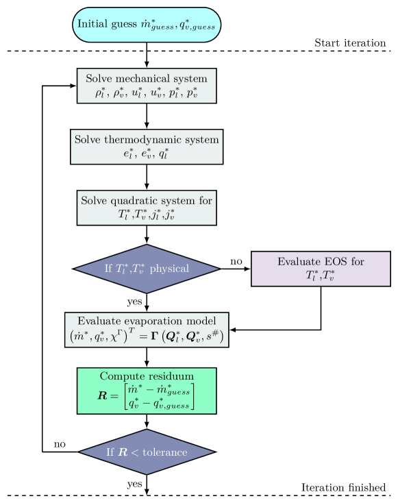
Figure 2: Flowchart, illustrating the iterative solution procedure of the $\text{HLLP}_{mq}$ Riemann solver.

An inherent issue of the quadratic equation system is the possibility of a negative discriminant during the iterative solution procedure when given inaccurate initial guesses for $\dot{m}^{*}$ and $\dot{q}^{*}$. Such behavior was encountered when computing more complex multi-dimensional setups involving severe phase interface deformations, surface tension and strong thermodynamic non-equilibrium. In the $\text{HLLP}_{mq}$ Riemann solver, we circumvent this issue with a fallback to an EOS evaluation for the temperatures, in case the discriminant exhibits a negative sign. The non-equilibrium contribution $\frac{1}{2}\alpha j^{2}$ to the total energy (6) is neglected during the EOS evaluation, since $j_{l}^{*}$ and $j_{v}^{*}$ are still unknown. We want to emphasize, that this fallback is only encountered during the initial iteration steps and not allowed in the final step. With the temperatures $T_{l}^{*}$ and $T_{v}^{*}$ known, we can finally obtain the thermal impulses from equations (53) and (55). The main steps during the iterative solution process of the $\text{HLLP}_{mq}$ solver are visualized in figure 2. The iterative solution procedure is illustrated in figure 2.

Notice, that equation (54) was not used in the solution procedure so far. To explain this curious decision, we want to recapitulate the effects of the relaxation source terms in the GPR model. In the balance equation for the thermal impulse (1d), the thermal relaxation source term controls the dissipation and therefore the entropy production due to heat conduction. Since the $\text{HLLP}_{mq}$ two-phase Riemann solver is formulated for the homogeneous GPR system, it would appear that we enforced a negligible entropy production across the interface. However, even if the thermal relaxation source terms had been included, the GPR model could not be expected to predict the correct entropy production in the presence of phase transition due to the breakdown of the continuum assumption across the phase boundary.

By incorporating a temperature jump $\Delta T$ in the jump relation (13d), we allow the phase transition model to impose an interfacial entropy production. In that sense the additional degree of freedom $\Delta T$ in the thermal impulse jump relation acknowledges the existence of an unknown thermal relaxation source term, that is determined through the local thermodynamic model. The proposed strategy thus allows a consistent coupling between the GPR model and a local thermodynamic phase transition model, that guides the iterative solution procedure to the correct entropy solution.

3.4.2 The $\text{HLLP}_{m}$ Two-Phase Riemann Solver

While the proposed $\text{HLLP}_{mq}$ interface Riemann solver combines the GPR model consistently with a thermodynamic closure relation, the iteration in the two variables poses a possible source for instabilities and increased computational costs. This motivates, the construction of a further simplified two-phase Riemann solver, called $\text{HLLP}_{m}$, which requires only an iteration in the mass flux $\dot{m}^{*}$. Since the linear mechanical system is evaluated independent of the heat flux $q_{v}^{*}$, the differences between the $\text{HLLP}_{mq}$ and $\text{HLLP}_{m}$ solvers are restricted to the construction of the thermodynamic system.

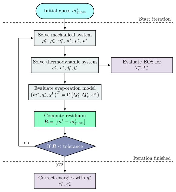
Figure 3: Flowchart, illustrating the iterative solution procedures of the $\text{HLLP}_{m}$ Riemann solver.

The iteration in $q_{v}^{*}$ is necessary since the jump relations for the energy across the three waves provide only three equations for the four unknown energies and heat fluxes $e_{l}^{*}$, $e_{v}^{*}$, $q_{l}^{*}$ and $q_{v}^{*}$. A possible simplification to obtain closure without a prediction of $q_{v}^{*}$ is to neglect the heat fluxes in the energy jump conditions across the outer waves. Equations (50) and (52) thus reduce to

$$\dot{m}_{l}e_{l}+u_{l}p_{l} =\dot{m}_{l}e_{l}^{*}+u_{l}^{*}p_{l}^{*},$$ (62)

$$\dot{m}_{v}e_{v}+u_{v}p_{v} =\dot{m}_{v}e_{v}^{*}+u_{v}^{*}p_{v}^{*}.$$ (63)

Consequently, they can be solved for the unknown energies $e_{l}^{*}$ and $e_{v}^{*}$ independently of the phase transition model. Subsequently, the temperatures $T_{l}^{*}$ and $T_{v}^{*}$ are determined by the EOS, while the non-equilibrium contributions $\frac{1}{2}\alpha j^{2}$ to the total energy (6) are neglected. Finally, with the temperatures known, the thermal impulses $j_{l}^{*}$ and $j_{v}^{*}$ are computed with equations (53) and (55). As depicted in figure 3, the simplified thermodynamic system allows to solve the two-phase Riemann problem with an iteration over the mass flux $\dot{m}^{*}$ only.

To account for the heat flux $q_{v}^{*}$, predicted by the evaporation model, a correction step is performed after the iteration in $\dot{m}^{*}$ has converged. Using the states $\boldsymbol{Q}^{*}_{l}$ and $\boldsymbol{Q}^{*}_{v}$ from the final iteration and the matching heat flux prediction $q_{v}^{*}$ from the evaporation model, the heat flux $q_{l}^{*}$ is computed via equation (51):

$$q_{l}^{*}=\dot{m}_{v}e_{v}^{*}+u_{v}^{*}p_{v}^{*}+q_{v}^{*}-(\dot{m}_{l}e_{l}^{*}+u_{l}^{*}p_{l}^{*}+s^{\#}\Delta p_{\sigma}).$$ (64)

When the heat fluxes $q_{v}^{*}$ and $q_{l}^{*}$ are available, the energies $e_{l}^{*}$, $e_{v}^{*}$ can finally be computed with (50) and (52), without neglecting the heat conduction across the outer waves, as done in (62) and (63). This correction step for the energies is crucial to achieve a solution, that is in agreement with the predicted thermodynamic flux $q_{v}^{*}$ of the evaporation model. The final solution procedure for the $\text{HLLP}_{mq}$ solver is outlined in figure 3.

4 Numerical Results

In this Section, we apply the proposed numerical method to a range of representative test cases. First, the thermal relaxation formulation of the GPR continuum model is compared against the Euler-Fourier system. Therefore, a one-dimensional heat conduction problem and the well-known Rayleigh-Bénard convection are studied. Next, the novel $\text{HLLP}_{mq}$ and $\text{HLLP}_{m}$ Riemann solvers are validated with evaporating shock tube computations against MD reference data and solutions obtained with the Euler-Fourier approach. The investigation focuses on a qualitative analysis, convergence studies and a comparison of the computational costs. Finally, we apply the method to shock-droplet interactions that involve phase transition, surface tension and complex deformations of the phase interface.

4.1 One-Dimensional Heat Conduction

In this paragraph, we investigate a one-dimensional heat conductivity dominated singe-phase flow to validate the thermal relaxation model of the GPR system against the Euler-Fourier model. We consider a computational domain $\Omega=[0,1]$ that contains a resting perfect gas with a constant temperature $T=2.0$ and pressure $p=2.5$ at the initial time $t=0.0$. Heat capacities at constant volume and pressure are chosen as $c_{v}=0.718$ and $c_{p}=1.005$ respectively and the relaxation time $\tau$ of the GPR model is defined according to (11). The setup is visualized in figure 4 with periodic boundary conditions in y-direction and heat fluxes $q^{+}$ and $q^{-}$ imposed at the lower and upper boundaries in x-direction. With the heat transmission coefficient $\alpha=100\lambda$, the heat fluxes are defined as

$$q^{+}=\rho\alpha(T-T_{B}^{+}),$$

$$q^{-}=\rho\alpha(T-T_{B}^{-}),$$

and depend on the density and temperature at the wall. The left wall is heated to a temperature $T_{B}^{+}=3$ and the right wall is cooled to a temperature $T_{B}^{-}=1$. Wherever not indicated, standard SI units can be assumed. The domain $\Omega$ is discretized with $[256]\times[1]$ DG elements of degree $N=2$. We perform three computations

Figure 4: Computational setup for the one-dimensional heat conduction test case. Heat fluxes are imposed on the left and right boundaries.

with different heat conductivities $\lambda=1\cdot 10^{-3}$, $\lambda=1\cdot 10^{-4}$ and $\lambda=1\cdot 10^{-5}$ until the final computation times $t=200$, $t=4000$ and $t=40000$ respectively. Figure 5 depicts the temperature profiles in x-direction at different time instances, computed with the GPR model and the Euler-Fourier system as a reference solution. A near-perfect agreement of both solutions can be observed for the considered range of thermal conductivities.

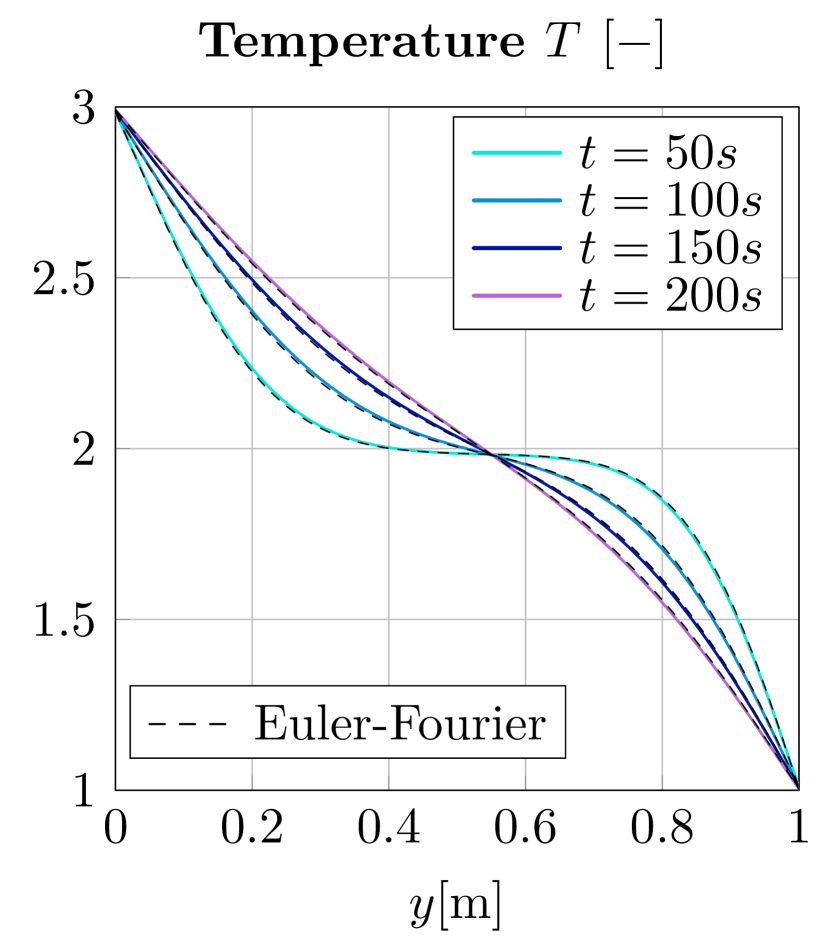
(a) $\lambda=1\cdot 10^{-3}$

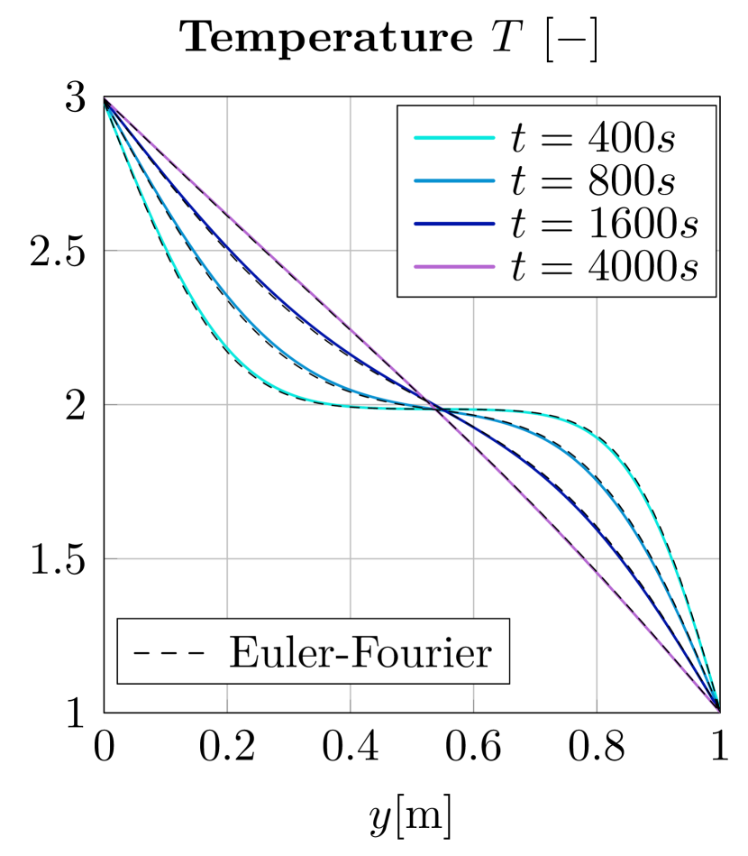
(b) $\lambda=1\cdot 10^{-4}$

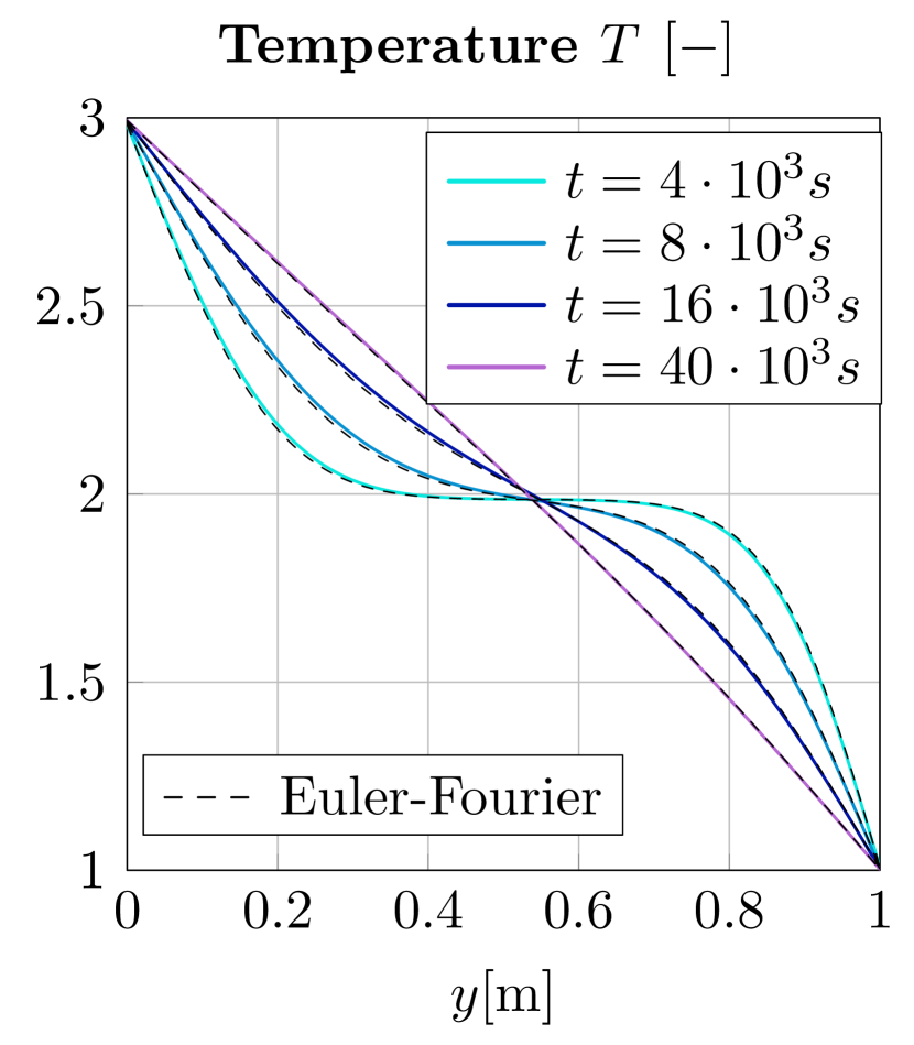
(c) $\lambda=1\cdot 10^{-5}$

Figure 5: Temperature profile of the one-dimensional heat conduction test case at different time instances. The heat conductivity is increased from left to right and the GPR model is compared against a Euler-Fourier reference solution.

4.2 Rayleigh-Bénard Convection

The Rayleigh-Bénard convection is a well-known benchmark, based on the interaction of heat conductivity and gravitational forces. In this paragraph, it is used as a two-dimensional test case to assess the computational performance of the present GPR implementation. As an initial setup, we consider a two-dimensional domain $\Omega=[0,1]\times[0,1]$ that contains a resting perfect gas with a constant temperature $T=2.0$. A gravitational force with gravitation constant $g=1.0$ is imposed in negative y-direction. For the compressible fluid, this results in a non-linear hydrostatic pressure profile

$$p(y)=p_{0}\exp{\left(\frac{gy}{T_{0}k}\right)}\quad\text{, with}\quad T_{0}=2.0,p_{0}=2.5,k=\frac{c_{p}}{c_{v}},$$ (65)

with $T_{0}=2.0$, $p_{0}=2.5$, $R=\frac{c_{p}}{c_{v}}$ and $c_{v}=0.718$ and $c_{p}=1.005$. Periodic boundary conditions are imposed in x-direction, while heat fluxes $q^{+}$ and $q^{-}$ are prescribed at the lower and upper boundaries in y-direction. The heat fluxes are defined similarly to Section 4.1 with the addition of a sine-shaped perturbation in x-direction

$$q^{+}=\rho h(T-T_{B}^{+})(1+0.1\text{cos}(8\pi x)),$$

$$q^{-}=\rho h(T-T_{B}^{-})(1+0.1\text{cos}(8\pi x)),$$

and the transmission coefficient $h=100\lambda$. We consider three different thermal conductivities $\lambda=1\cdot 10^{-3}$, $\lambda=1\cdot 10^{-4}$ and $\lambda=1\cdot 10^{-5}$ and chose the thermal relaxation time $\tau$ according to equation (11). Since we study the inviscid GPR model in the present work, viscosity is neglected. The final setup is depicted in figure 6

Figure 6: Computational setup for the Rayleigh-Bénard convection test case.

and discretized with $256\times 256$ DG elements of degree $N=3$ in a time interval $t\in[0,40]$. We compare the results obtained with the GPR continuum model with Euler-Fourier computations. Since we neglect physical viscosity, the gravitational forces are solely damped by numerical viscosity. Therefore, the characteristic convection process of the Rayleigh-Bénard instability develops, as visualized in figure 7.

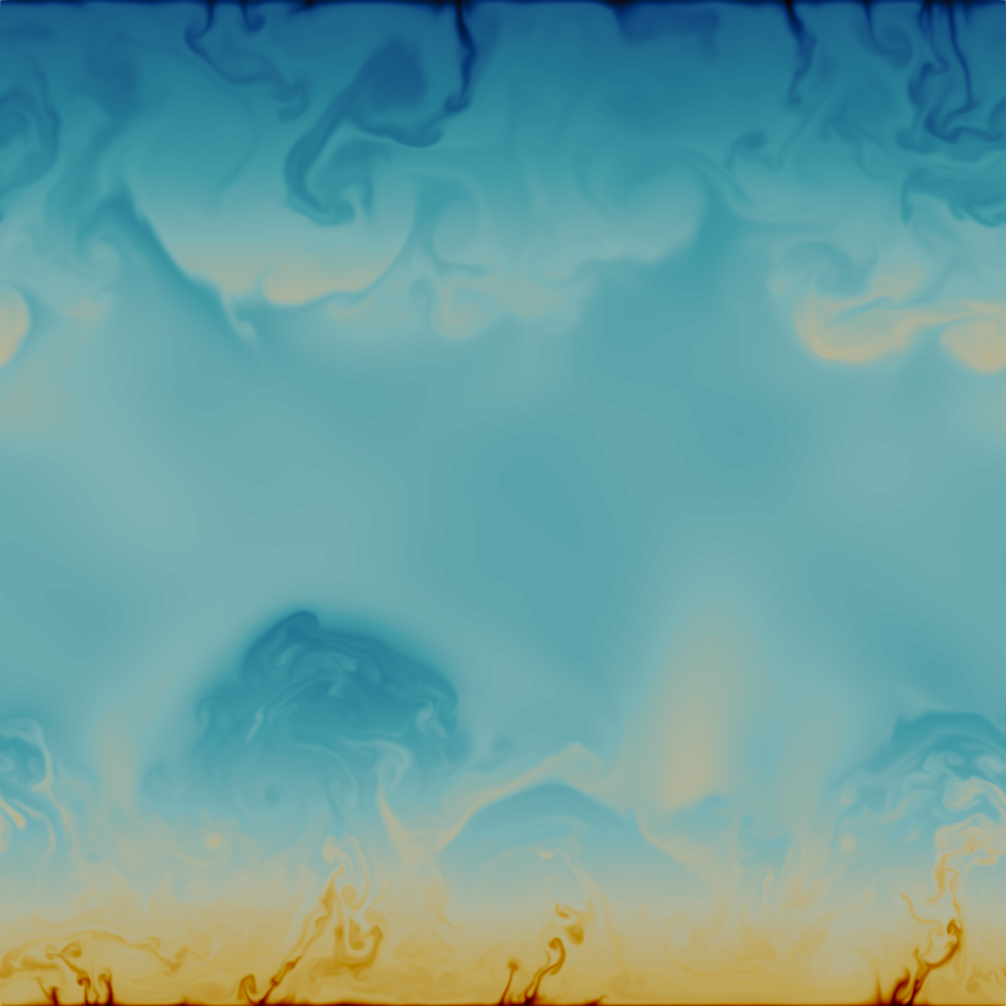
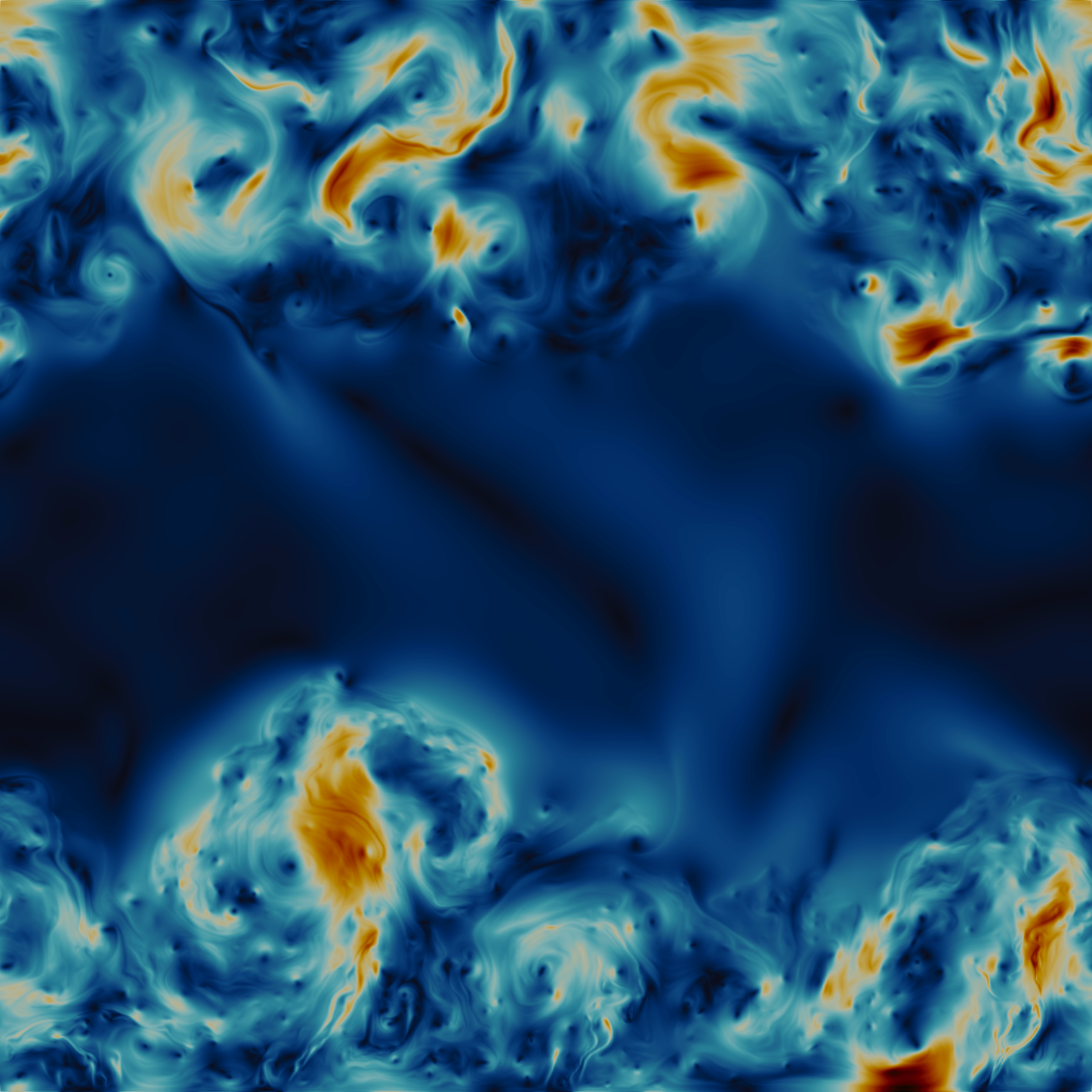
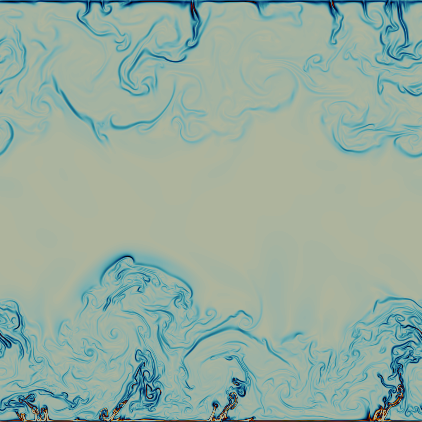
(a) Temperature

(b) Velocity magnitude

(c) Thermal impulse magnitude

Figure 7: Temperature (left), velocity (center) and thermal impulse (left) field of a Rayleigh-Bénard convection at $t=40.0$ with $\lambda=1\cdot 10^{-5}$, computed with the GPR continuum model.

For a quantitative comparison between the GPR and Euler-Fourier model, temperature profiles in y-direction are averaged along the x-axis at the final computation time $t=40.0$. The resulting temperature statistics are visualized in figure 8 and show a good agreement.

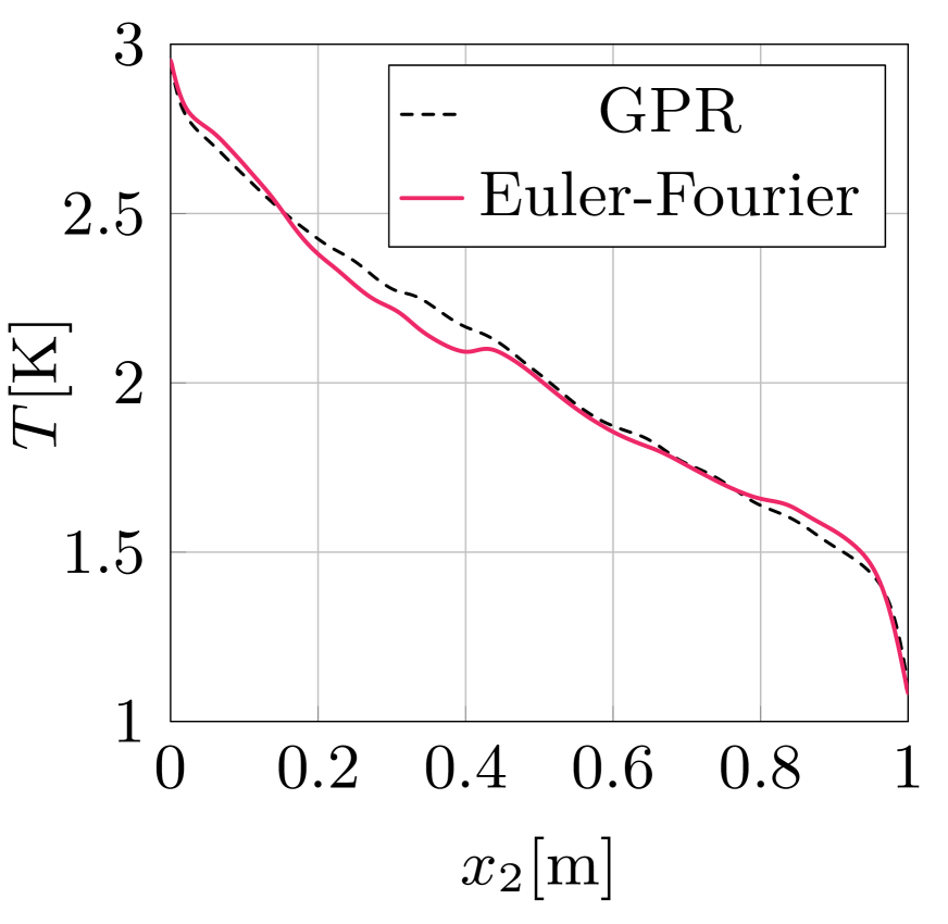
(a) $\lambda=1\cdot 10^{-3}$

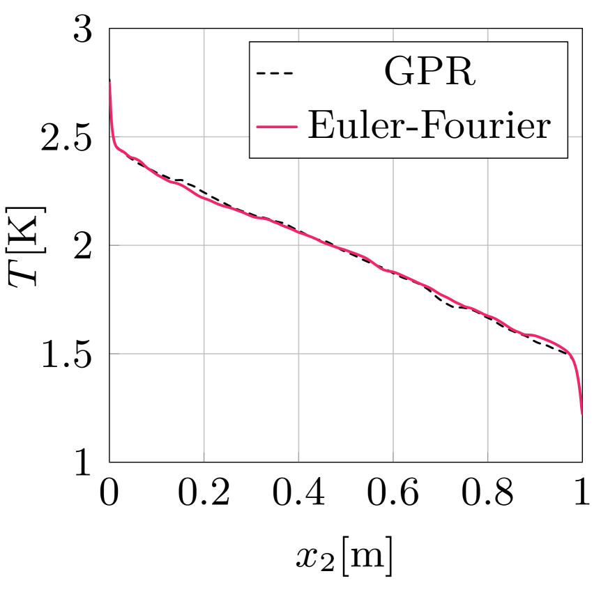
(b) $\lambda=1\cdot 10^{-4}$

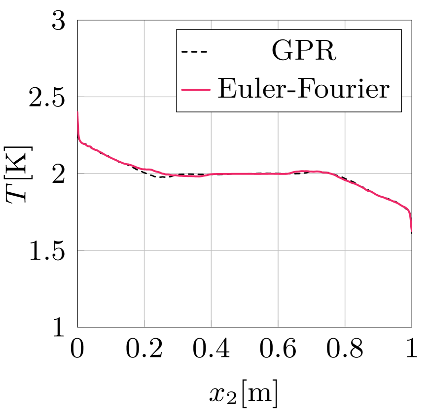
(c) $\lambda=1\cdot 10^{-5}$

Figure 8: Temperature profiles in y-direction, averaged over the x-direction for different thermal conductivities $\lambda$. The GPR computation is compared against a reference solution, obtained with the Euler-Fourier system.

To quantify the computational efficiency of both schemes, we compare the wall time and the total number of time steps in table 1.

	$\lambda$	Time steps	Wall time [CPU h]
GPR	$1\cdot 10^{-3}$	$1.76\cdot 10^{5}$	743.8
Euler-Fourier		$5.13\cdot 10^{5}$	1910.6
GPR	$1\cdot 10^{-4}$	$1.69\cdot 10^{5}$	623.0
Euler-Fourier		$1.69\cdot 10^{5}$	468.5
GPR	$1\cdot 10^{-5}$	$1.58\cdot 10^{5}$	618.8
Euler-Fourier		$1.56\cdot 10^{5}$	432.7

Table 1: Comparison of the number of times steps and the wall time for the Rayleigh-Bénard convection benchmark with the GPR model and the Euler-Fourier system.

For the lower heat conductivities $\lambda=1\cdot 10^{-4}$ and $\lambda=1\cdot 10^{-5}$, the number of time steps is nearly identical for both methods. A different trend is observed for the highest thermal conductivity $\lambda=1\cdot 10^{-3}$. Here, the Euler-Fourier computation requires about three times more time steps than the GPR computation. This behavior is a result of the parabolic time step constraint of the Euler-Fourier model, which is linked to the thermal diffusivity $d_{\alpha}=\frac{\lambda}{\rho c_{p}}$. Since the hyperbolic GPR model avoids this constraint, it outperforms the Euler-Fourier model in the presence of high thermal conductivities. In contrast, when the time step is restricted by the convective process, the GPR model requires about $30\%$ more wall time due to the additional variables for the thermal impulse.

4.3 Evaporating LJTS Shock-Tube

To validate the $\text{HLLP}_{mq}$ and $\text{HLLP}_{m}$ two-phase Riemann solvers, we study an evaporating shock tube setup, introduced by Hitz et al. [31]. It is defined as a Riemann problem for the LJTS fluid with piece-wise constant initial conditions

$$\boldsymbol{Q}(\boldsymbol{x},0)=\begin{cases}(\rho,u,T)^{T}=(0.6635,0.0,0.9)^{T}&\quad\text{, for}\;x<0\;\text{(liq)},\\ (\rho,u,T)^{T}=(0.013844,0.0,0.8)^{T}&\quad\text{, for}\;x>0\;\text{(vap)},\end{cases}$$

within a computational domain $\Omega=[-200,1000]$. The left state is in a saturated liquid state, while the right state consists of superheated vapor. The initial conditions are provided in non-dimensionalized form with the reference length $\sigma_{\text{ref}}=1\text{\AA}$, the reference energy $\frac{\epsilon_{\text{ref}}}{k_{B}}=1K$, the reference mass $m_{\text{ref}}=1u$ and the reference time $t_{\text{ref}}=\sigma_{\text{ref}}\sqrt{m_{\text{ref}}/\epsilon_{\text{ref}}}$ following Merker et al. [50]. We apply the EOS of Heier et al. [28] for the LJTS fluid and model the heat conductivities in the liquid and vapor with the models of Lautenschläger and Hasse [44] and Lemmon and Jacobsen [46], respectively. The thermal relaxation time $\tau$ is defined by equation (12) according to a thermomass theory model. We discretize the computational domain with $N_{\text{elems}}=300$ DG elements of degree $N=3$. In the presence of shocks or the phase boundary, the FV sub-cell scheme with a sub-cell resolution of $N_{FV}=4$ is applied. The setup is computed until a final time $t=600$.

In figure 9, we compare the solutions of the introduced $\text{HLLP}_{mq}$ and $\text{HLLP}_{m}$ Riemann solvers to Euler-Fourier computations by Jöns et al. [33] and a molecular dynamics simulation of Hitz et al. [31].

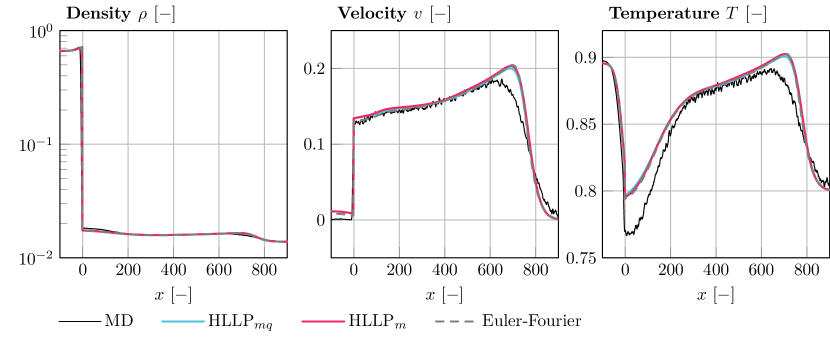
Figure 9: Density, velocity and temperature of the evaporating LJTS shock tube at time $t=600$. The $\text{HLLP}_{mq}$ and $\text{HLLP}_{m}$ Riemann solvers are compared against the Euler-Fourier solution of Jöns et al. [33] and a reference solution from molecular dynamic data of Hitz et al. [31].

An excellent agreement between the solutions of the $\text{HLLP}_{mq}$ and $\text{HLLP}_{m}$ Riemann solvers can be observed. Further, the GPR computations match the solution of the Euler-Fourier system almost perfectly.

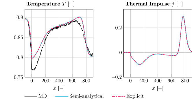
Figure 10: Comparison of the temperature and thermal impulse distribution at $t=600$ computed with a semi-analytical and explicit source term integration scheme.

When compared against the molecular dynamics data, the $\text{HLLP}_{mq}$ and $\text{HLLP}_{m}$ solvers show a good qualitative agreement. Deviations are most prominent at the phase boundary, where the GPR computations slightly overpredict the temperature. A possible cause for the discrepancy could be an underprediction of the evaporation by the thermodynamic closure model. Deviations between the GPR results and the MD data away from the interface can be explained by the fact that in this work we neglected viscous effects.

Next, the semi-analytical source term integration scheme of Section 3.3 is validated. Therefore, the shock tube computation is repeated with an explicit source term integration scheme. Due to the high thermal diffusivity $d_{\alpha}=\frac{\lambda}{\rho c_{p}}$ of the LJTS fluid, the thermal relaxation time obtained with equation (12) leads to a mildly stiff behavior of the source and an explicit reference computation is affordable. Both methods are compared in figure 10 and demonstrate a near-perfect agreement in the temperature and thermal impulse profiles.

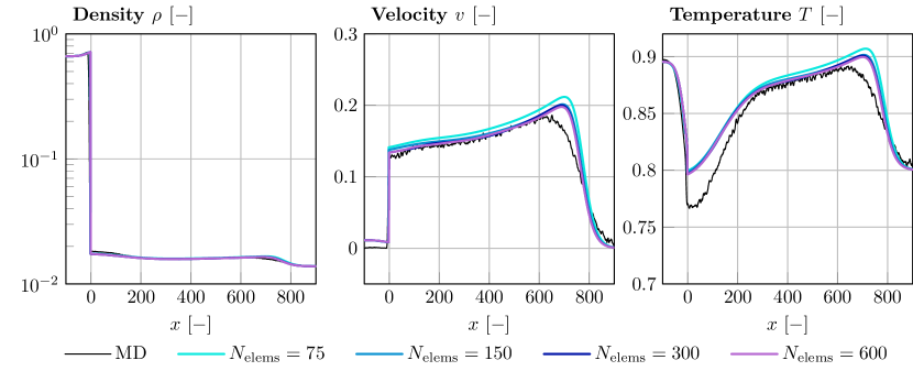
Figure 11: Mesh convergence study with the $\text{HLLP}_{mq}$ two-phase Riemann solver for an evaporating LJTS shock tube.

Further, a mesh convergence study is performed for the evaporating shock tube in figure 11. Therefore, the computation is repeated for a range of mesh resolutions $N_{\text{elems}}\in[75,150,300,600]$. With an increased resolution, a noticeable decrease in the vapor temperatures and velocities is observable. Beyond a resolution of $N_{\text{elems}}=300$, a further increase in the element number has only a very minor effect on the solution.

Finally, the computational efficiency of the GPR method is assessed in comparison to the Euler-Fourier methodology. Since the LJTS fluid exhibits a high thermal conductivity $\lambda$ and consequently high thermal diffusivity $d_{\alpha}$, the Euler-Fourier scheme suffers from a parabolic time step restriction. As indicated in table 2, this results in significantly larger computation times due to an increased number of time steps when compared to the GPR model.

In summary, the introduced $\text{HLLP}_{mq}$ and $\text{HLLP}_{m}$ Riemann solvers provide results in good agreement with MD reference data. A comparison to a sharp interface study with the Euler-Fourier method revealed a significant performance advantage of the GPR method due to a lack of a parabolic time step constraint. Further, a mesh convergence study achieves convergence at a reasonable resolution. Finally, a perfect agreement between the semi-analytical source term integration and an explicit reference solution was demonstrated.

	Time steps	Wall time [CPU h]
GPR $\text{HLLP}_{mq}$	$3.76\cdot 10^{3}$	29.7
Euler-Fourier	$3.50\cdot 10^{4}$	197.9

Table 2: Comparison of the number of times steps and the wall time for the evaporating LJTS shock tube with the GPR model and the Euler-Fourier system.

4.4 Evaporating n-Dodecane Shock-Tube

In the previous paragraph, we investigated an evaporating shock tube for an artificial model fluid, derived from the LJTS potential. This facilitated a validation against molecular dynamics simulations to establish the proposed interfacial Riemann solvers. With this Section, we extend the study to a shock tube problem for the material n-Dodecane. A Riemann problem is derived from an evaporating n-Dodecane shock-droplet setup, reported by Jöns et al. [33], with piecewise constant initial liquid and vapor states

$$\boldsymbol{Q}(\boldsymbol{x},0)=\begin{cases}(\rho,u,p)^{T}=(539.94[\frac{Kg}{m^{3}}],0.0[\frac{m}{s}],0.13[\text{MPa}])^{T}&\text{, for}\;x<0\;\text{(liq)},\\ (\rho,u,p)^{T}=(4.3830[\frac{Kg}{m^{3}}],0.0[\frac{m}{s}],0.10[\text{MPa}])^{T}&\text{, for}\;x>0\;\text{(vap)},\end{cases}$$

separated by a phase boundary at $x=0$. N-dodecane is modeled with the Peng-Robinson EOS, based on the material parameter listed in table 3. The thermal conductivity is determined with the model of Chung et al. [13]. We chose the thermal relaxation time $\tau$ according to equation (11).

$\rho_{c}[\frac{Kg}{m^{3}}]$	$p_{c}[\text{MPa}]$	$T_{c}[K]$	$M[\frac{Kg}{mol}]$	$\omega[-]$
226.55	18.17	658.1	0.1703	0.576

Table 3: Material parameter of the Peng-Robinson EOS for n-Dodecane

The setup considers a domain $\Omega=[0,0.001]\mathrm{m}$ that is discretized with $600$ DG elements of degree $N=3$. At shocks and the interface, a local refinement is applied based on an FV sub-cell scheme with a resolution of $N_{FV}=4$ sub-cells per DG element. The setup is advanced until a final computation time $t=2\cdot 10^{-6}\mathrm{s}$ with the novel $\text{HLLP}_{mq}$ and $\text{HLLP}_{m}$ interface solvers.

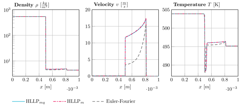
Figure 12: Density, velocity and temperature profile of an evaporating shock tube computation with the material n-Dodecane at $t=2\cdot 10^{-6}\mathrm{s}$. Sharp interface computations with the $\text{HLLP}_{mq}$ and $\text{HLLP}_{m}$ solvers are compared against an Euler-Fourier solution.

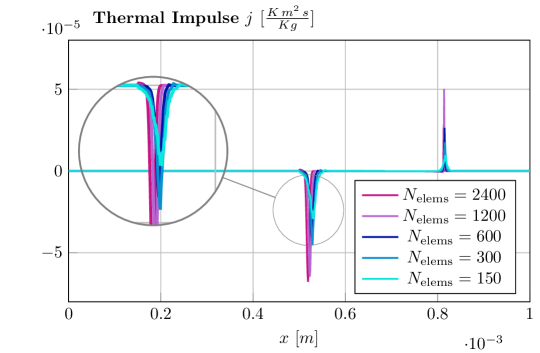
Figure 13: Convergence study with the $\text{HLLP}_{mq}$ solver for the thermal impulse $j$.

Figure 12 provides the density, velocity and temperature profiles at the final time $t=2\cdot 10^{-6}\mathrm{s}$. Results, obtained with the GPR model are compared against an Euler-Fourier reference solution, computed with the framework of Jöns et al. [33]. While an excellent agreement can be observed between the novel $\text{HLLP}_{mq}$ and $\text{HLLP}_{m}$ two-phase Riemann solvers, the Euler-Fourier solution predicts a significantly lower velocity in the vapor and a sharper temperature jump at the interface. The wider temperature profile indicates a more dissipative behavior of the GPR model, compared to the Euler-Fourier system.

This observation can be explained by the thermal impulse distribution, visualized in figure 13. Due to low significantly lower thermal conductivity of n-Dodecane compared to the LJTS fluid, steep gradients in the temperature cause a delta-pulse-like distribution of the thermal impulse. Capturing these sharp solution features is demanding for a discretization scheme and incurs a particularly high resolution requirement. This argument is further supported by a mesh convergence study in figure 14. Similar observations were reported by Peshkov et al in [59] with regard to the simulation of viscous flows in the GPR framework.

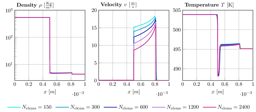
Figure 14: Mesh convergence study with the $\text{HLLP}_{mq}$ two-phase Riemann solver for an evaporating n-Dodecane shock tube.

While mesh convergence is not reached for the GPR model at $N_{\text{elems}}=2400$, the investigation suggests that the solution approaches the Euler-Fourier reference with increasing mesh resolution. This trend is particularly pronounced in the velocity of the freshly evaporated vapor. Furthermore, the temperature dip at the phase boundary appears sharper with increasing mesh resolutions.

Next, we analyze the accuracy of the semi-analytical integration scheme for the thermal relaxation source term. Again, a reference solution is computed with an explicit source term integration scheme. Due to the prohibitive time step restriction of the explicit scheme, the comparison is performed for a coarse resolution of $N_{\text{elems}}=150$ elements and evaluated at $t=7\cdot 10^{-8}\mathrm{s}$. Figure 15 depicts the temperature and thermal impulse profiles for both simulations.

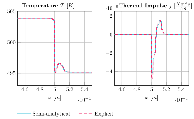
Figure 15: Comparison of the temperature profile and thermal impulse distribution for the semi-analytical and explicit integration of the thermal relaxation source term.

Both schemes produce near identical results with a slightly damped thermal impulse profile obtained with the semi-analytical scheme.

Finally, the computational costs of the GPR computation and the Euler-Fourier reference are evaluated in table 4. For the given thermal conductivity of n-Dodecane, the time step is dominated by the convection process and the parabolic time step constraint of the Euler-Fourier system has no effect. Thus both schemes require roughly the same number of times steps. The increased wall time of the GPR implementation is the result of the additional variables for the thermal impulse and the source term integration.

	Time steps	Wall time [CPU h]
GPR $\text{HLLP}_{mq}$	$2.89\cdot 10^{3}$	49.5
Euler-Fourier	$2.80\cdot 10^{3}$	16.0

Table 4: Comparison of the number of times steps and the wall time for the evaporating n-Dodecane shock tube with the GPR model and the Euler-Fourier system.

In conclusion, the low thermal conductivity of n-Dodecane compared to the LJTS fluid results in low thermal diffusivity. As a consequence, the solution exhibits sharp temperature gradients, that cause delta-pulse-like solution features in the thermal impulse. Therefore, a particularly high-resolution requirement is observed for GPR computations. Since the Euler-Fourier system does not suffer from a parabolic time step restriction in this case, it proves to be the more efficient method for the given setup.

4.5 Shock-Droplet Interaction

Finally, we consider a two-dimensional shock-droplet interaction with phase transition for n-Dodecane. The test case involves surface tension and severe phase boundary deformations and is chosen in order to demonstrate the robustness and efficiency of the proposed two-phase Riemann solver for complex two-phase simulations. We adopt a setup, proposed by Fechter et al. [22] and recently studied by Jöns et al. [33] as a test case for their Euler-Fourier two-phase Riemann solver. The computational domain $\Omega=[-2.5,7.5]\mathrm{mm}\times[-5.0,5.0]\mathrm{mm}$ contains a planar incident shock at $x=-1.5\mathrm{mm}$ and an initially resting droplet of radius $r=1.\mathrm{mm}$ at $x=0.\mathrm{mm}$ under evaporating conditions. The surface tension is set to $\sigma_{c}=0.009\mathrm{N}\,\mathrm{m}^{-1}$ resulting in a Weber number of $We=25549$. The setup is illustrated in figure 16(a) and initial conditions are provided in table 5. As an extension to the setup of Fechter et al. [22], we consider a second test case with a vapor-filled cavity of radius $r=0.5\mathrm{mm}$ inside the droplet, sketched in figure 16(b).

(a) Setup 1

(b) Setup 2

Figure 16: Initial setup for a 2D shock-droplet interaction. Setup 1 considers an initially resting n-Dodecane droplet. Setup 2 is an extension of setup 1 with the droplet containing a vapor-filled cavity.

	$\rho[\text{kg}\,\text{m}^{-3}]$	$u_{1}[\mathrm{m}\,\mathrm{s}^{-1}]$	$p[\mathrm{MPa}]$
Vapor (pre-shock) $\Omega_{v}$	4.383	0.0	0.10
Vapor (post-shock) $\Omega_{v_{s}}$	9.696	108.87	0.227
Vapor (cavity) $\Omega_{v_{c}}$	4.383	0.0	0.10
Liquid $\Omega_{l}$	539.94	0.0	0.13

Table 5: Initial conditions of the evaporating n-Dodecane shock-droplet interaction.

The computational domain $\Omega$ is discretized by $240\times 120$ DG elements with a polynomial degree in a range of $N=[2,4]$ and a FV sub-cell resolution of $N_{FV}=9$. The sharp phase interface is always discretized by FV sub-cells, leading to an effective resolution of $432$ DOFs per bubble diameter. Due to the symmetric setup, we only compute half of the domain $\Omega$ and impose symmetry boundary conditions along the x-axis. For the remaining boundaries, we impose non-reflecting boundary conditions at the right and top and an inflow boundary condition at the left. The numerical flux is computed by an HLLC Riemann solver in the bulk and by the $\text{HLLP}_{mq}$ Riemann solver at the phase interface.

(a) $t=10\mu\mathrm{s}$

(b) $t=30\mu\mathrm{s}$

(c) $t=60\mu\mathrm{s}$

(d) $t=100\mu\mathrm{s}$

Figure 17: Numerical schlieren images analyzed temperature fields of an n-Dodecane shock-droplet interaction with phase transition using the $\text{HLLP}_{mq}$ two-phase Riemann solver.

We advance the setup until a final time $t=120\mu\mathrm{s}$. The computation is performed on $1024$ processor units and load imbalances caused by the adaptive discretization, the interface tracking and the two-phase Riemann solver are balanced with the dynamic load balancing (DLB) scheme, introduced in [5, 52].

Figure 17 provides numerical schlieren images and the temperature fields of the shock-droplet interaction at times $t=10\mu\mathrm{s}$, $t=30\mu\mathrm{s}$, $t=60\mu\mathrm{s}$ and $t=100\mu\mathrm{s}$.

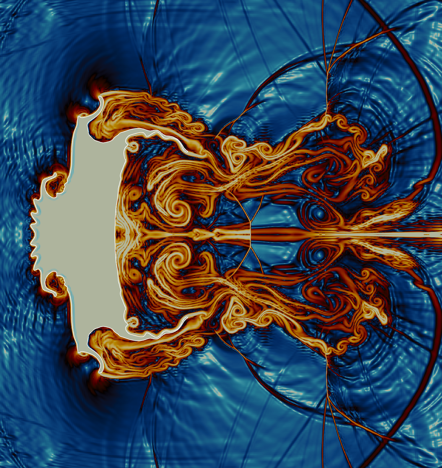
(a) Thermal impulse $|\rho\boldsymbol{j}|$

(b) Adaptive discretization

Figure 18: The left plot shows the absolute thermal impulse $|\rho\boldsymbol{j}|$ at time $t=100\mu\mathrm{s}$. The bottom half of the right figure shows the hp-adaptive hybrid DG/FV discretization. The top half depicts the current partition of the domain and indicates the number of elements per processor.

Results are in good qualitative agreement with the reported computations of Jöns et al. [33]. At $t=10\mu\mathrm{s}$, the incident shock wave passed through most of the droplet and has been reflected at the droplet surface. Inside the droplet, the transmitted wave is reflected at the back and a weak retransmitted wave behind the droplet is observable. Due to the initial pressure difference between the droplet and the surrounding vapor, a circular shock wave has formed around the droplet and interacts with the incident shock. At the droplet surface, still unaffected by the incident shock, a lower temperature in the vapor is visible due to the latent heat of the evaporating droplet.

At the front of the droplet, a slight increase in the droplet temperature is visible. We follow the explanation of Jöns et al. and Fechter et al. [22, 33] and assume that this phenomenon is caused by the condensation of hot vapor impinging on the cool droplet surface. At $t=30\mu\mathrm{s}$, the onset of instabilities at the droplet surface due to the high Weber number becomes apparent. They develop into filaments at $t=60\mu\mathrm{s}$ and grow until they almost detach from the main liquid body at $t=100\mu\mathrm{s}$. During later stages of the simulation, condensation at the front of the droplet becomes stronger, indicated by a heating of the surface. In the back of the droplet, freshly evaporated and cooled vapor detaches and mixes with vortical structures in the wake of the droplet. Since the GPR continuum model is used for the bulk fluid, heat conduction is modeled through the thermal impulse. As visualized in figure 18(a), the absolute value of the thermal impulse is an excellent choice for the visualization of temperature gradients in the fluid.

(a) $t=10\mu\mathrm{s}$

(b) $t=40\mu\mathrm{s}$

(c) $t=45\mu\mathrm{s}$

(d) $t=60\mu\mathrm{s}$

Figure 19: Interaction of an incident shock wave with an evaporating n-Dodecane droplet that contains a vapor-filled cavity. Numerical results, obtained with the $\text{HLLP}_{mq}$ two-phase Riemann solver show a collapse of the cavity.

Finally, insight into the adaptive discretization and DLB is provided by figure 18(b). The lower half of the plot indicates regions where FV sub-cell limiting and p-refinement is applied. Shocks and the phase interface are detected and treated with the refined FV sub-cell grid. At vortical structures in the wake of the droplet, a higher polynomial degree is applied to reduce numerical dissipation. The upper half of figure 18(b) highlights the partition of the computational domain due to DLB. With processor units receiving between $1$ and $64$ elements, a substantial load imbalance between elements can be constituted. Elements discretized by the FV sub-cell scheme or the DG scheme with an increased polynomial degree have the highest cost.

As a final test case, we consider the extended setup with a vapor-filled cavity inside the droplet. At $t=10\mu\mathrm{s}$ a very similar result is observed. However, the transmitted incident shock wave is now reflected at the surface of the cavity inside the droplet. Here, a temperature drop can be observed due to the evaporation of the liquid droplet into the vapor of the cavity. Between $t=10\mu\mathrm{s}$ and $t=40\mu\mathrm{s}$, the bubble undergoes a significant deformation caused by the formation of a high-speed liquid jet along the $y=0$ axis. This liquid jet leads to a bubble collapse at $t=45\mu\mathrm{s}$, with shock waves of the collapse reflected at the back of the droplet. The high pressure in the primary cavity and in the secondary cavities, formed after the collapse, causes condensation. This leads to a slight increase in the liquid temperature at the surface of the primary and secondary cavities during and after the collapse.

In summary, the two-dimensional shock-droplet interactions demonstrate the applicability of the proposed $\text{HLLP}_{mq}$ Riemann solver to complex two-phase simulations with phase transition in the presence of surface tension and significant interface deformations.

5 Conclusion

In this paper, we presented a sharp interface approach for the simulation of compressible two-phase flows with phase transition. It employs the first-order hyperbolic continuum model of Godunov, Peshkov and Romenski to describe compressible, inviscid heat-conducting fluid flow in the bulk phases. The main contribution of this work is the construction of two novel interfacial Riemann solvers that provide a thermodynamically consistent coupling at the phase boundary in the presence of phase transition. The developed Riemann solvers address two key challenges related to the modeling of phase transition in the sharp interface context: a loss of self-similarity due to irreversible effects at the interface like entropy production and heat conduction and avoiding the breakdown of the continuum assumption across the phase boundary. Using the hyperbolic GPR model, irreversible effects are treated as relaxation processes and confined to a source term. To obtain a unique and thermodynamically consistent entropy solution, we employ a local phase transition model to determine the source term and thus predict the entropy production and heat dissipation associated with phase transition.

The novel interfacial solvers are constructed from integral jump relations across a simplified wave fan, analogously to the established HLLC methodology. The equation system is closed by a kinetic relation that employs an entropy estimate from a kinetic theory-based phase transition model. With phenomenological force flux relations of Onsager theory, the entropy production is related to the interfacial mass and heat flux. The resulting non-linear equation system can be solved iteratively. We propose two approximate solvers for the two-phase Riemann problem denoted $\text{HLLP}_{mq}$ and $\text{HLLP}_{m}$. While the $\text{HLLP}_{mq}$ solver relies on an iterative solution in both the mass and heat flux, the simplified $\text{HLLP}_{m}$ solver requires only an iteration in the mass flux. In addition, we discussed the treatment of the thermal relaxation source term of the GPR model. We implemented a recently developed semi-analytical scheme [11] that allows to reproduce the Fourier law in the stiff relaxation limit.

To validate the presented method, we investigated a range of representative test cases. First, we compared the inviscid, heat-conducting GPR model against Euler-Fourier computations for heat-driven single-phase flows. An excellent agreement between both methods is observed while the GPR model demonstrates a superior computational efficiency in the presence of large heat conductivities due to the lack of a parabolic time step constraint. The two-phase Riemann solvers are validated against molecular dynamics data for an evaporating shock tube simulation with the Lennard-Jones shifted and truncated potential. Both the $\text{HLLP}_{mq}$ and $\text{HLLP}_{m}$ solvers yield near-identical results and match the molecular dynamics reference data well. Further, a close agreement with an analog Euler-Fourier computation is reported. Due to the high thermal conductivity of the LJTS-fluid, the GPR model is computationally advantageous, since it is not restricted by a parabolic time step constraint. As an additional test case, we studied an evaporating n-Dodecane shock tube. While the $\text{HLLP}_{mq}$ and $\text{HLLP}_{m}$ solver produce again near-identical solutions, the GPR results deviated significantly from the Euler-Fourier reference. The authors contribute this to a lack of resolution, required for the thermal impulse in case of low thermal conductivities. This assumption is supported by mesh convergence studies, suggesting a slow convergence against the Euler-Fourier result.

Finally, we applied the framework to two-dimensional shock-droplet interactions with phase transition. The setups feature surface tension, severe interface deformations and topological changes of the phase boundary. To meet the high local resolution requirement at the interface, the developed phase transition kernel was combined with the hp-adaptive discretization scheme, introduced in [53, 52]. A robust performance of the proposed interface Riemann solvers was demonstrated for complex simulations and a good qualitative agreement with similar shock-droplet investigations with the Euler-Fourier method [33] was achieved.

In the future, we extend the presented framework towards multi-component flows. This allows for validation against experiments with an evaporating liquid in an inert gaseous atmosphere. Therefore, the bulk phases need to accommodate species transport and diffusion, while the phase transition models need to be extended to the presence of a multi-component mixture.

Declarations

Funding We gratefully acknowledge the support of the German Research Foundation (DFG) for the research reported in this publication through the project ”Droplet Interaction Technologies”, grant GRK 2160/1 and GRK 2160/2 (project 270852890), the framework of the research unit FOR 2895 (grant BE 6100/3-1) and through Germany’s Excellence Strategy EXC 2075 (project 390740016).

Further, S. Chiocchetti acknowledges funding from the European Union’s Horizon Europe research and innovation program under project MoMeNTUM, Marie Skłodowska-Curie grant (agreement No. 101109532).

All simulations were performed on the national supercomputer HPE Apollo Systems HAWK at the High Performance Computing Center Stuttgart (HLRS) under the grant number hpcmphas/44084.

Conflict of interest The corresponding author states on behalf of all authors, that there is no conflict of interest.

Code availability The open-source code FLEXI, on which all extensions are based, is available at www.flexi-project.org under the GNU GPL v3.0 license.

Availability of data and material All data generated or analyzed during this study are included in this published article.

References

- [1] Abeyaratne, R., Knowles, J.K.: Kinetic relations and the propagation of phase boundaries in solids. Archive for Rational Mechanics and Analysis 114(2), 119–154 (1991). DOI 10.1007/bf00375400
- [2] Abgrall, R., Busto, S., Dumbser, M.: A simple and general framework for the construction of thermodynamically compatible schemes for computational fluid and solid mechanics. Applied Mathematics and Computation 440, 127629 (2023). DOI 10.1016/j.amc.2022.127629
- [3] Adalsteinsson, D., Sethian, J.A.: A fast level set method for propagating interfaces. Journal of Computational Physics 118(2), 269–277 (1995). DOI 10.1006/jcph.1995.1098
- [4] Anderson, D.M., McFadden, G.B., Wheeler, A.A.: Diffuse-interface methods in fluid mechanics. Annual Review of Fluid Mechanics 30(1), 139–165 (1998). DOI 10.1146/annurev.fluid.30.1.139
- [5] Appel, D., Jöns, S., Keim, J., Müller, C., Zeifang, J., Munz, C.D.: A narrow band-based dynamic load balancing scheme for the level-set ghost-fluid method. In: W.E. Nagel, D.H. Kröner, M.M. Resch (eds.) High Performance Computing in Science and Engineering ’21, pp. 305–320. Springer International Publishing, Cham (2023)
- [6] Baer, M., Nunziato, J.: A two-phase mixture theory for the deflagra-tion-to-detonation transition (ddt) in reactive granular materials. International Journal of Multiphase Flow 12(6), 861–889 (1986). DOI 10.1016/0301-9322(86)90033-9
- [7] Boscheri, W., Chiocchetti, S., Peshkov, I.: A cell-centered implicit-explicit lagrangian scheme for a unified model of nonlinear continuum mechanics on unstructured meshes. Journal of Computational Physics 451, 110852 (2022). DOI 10.1016/j.jcp.2021.110852
- [8] Boscheri, W., Loubére, R., Braeunig, J.P., Maire, P.H.: A geometrically and thermodynamically compatible finite volume scheme for continuum mechanics on unstructured polygonal meshes (2023)
- [9] Castro, M., Gallardo, J., Parés, C.: High order finite volume schemes based on reconstruction of states for solving hyperbolic systems with nonconservative products. Applications to shallow-water systems. Mathematics of Computation 75(255), 1103–1134 (2006)
- [10] Chester, M.: Second sound in solids. Physical Review 131(5), 2013–2015 (1963). DOI 10.1103/physrev.131.2013
- [11] Chiocchetti, S., Dumbser, M.: An exactly curl-free staggered semi-implicit finite volume scheme for a first order hyperbolic model of viscous two-phase flows with surface tension. Journal of Scientific Computing 94, 24 (2023). DOI 10.1007/s10915-022-02077-2
- [12] Chiocchetti, S., Mueller, C.: A Solver for Stiff Finite-Rate Relaxation in Baer–Nunziato Two-Phase Flow Models, pp. 31–44 (2020). DOI 10.1007/978-3-030-33338-6“˙3
- [13] Chung, T.H., Ajlan, M., Lee, L.L., Starling, K.E.: Generalized multiparameter correlation for nonpolar and polar fluid transport properties. Industrial & Engineering Chemistry Research 27, 671–679 (1988)
- [14] Cipolla, J.W., Lang, H., Loyalka, S.K.: Kinetic theory of condensation and evaporation. II. The Journal of Chemical Physics 61(1), 69–77 (1974). DOI 10.1063/1.1681672
- [15] Dang, L.X., Chang, T.M.: Molecular dynamics study of water clusters, liquid, and liquid–vapor interface of water with many-body potentials. The Journal of Chemical Physics 106(19), 8149–8159 (1997). DOI 10.1063/1.473820
- [16] Davis, S.F.: Simplified second-order Godunov-type methods. Siam Journal on Scientific and Statistical Computing 9, 445–473 (1988)
- [17] Dumbser, M., Loubère, R.: A simple robust and accurate a posteriori sub-cell finite volume limiter for the discontinuous Galerkin method on unstructured meshes. Journal of Computational Physics 319, 163–199 (2016). DOI 10.1016/j.jcp.2016.05.002
- [18] Dumbser, M., Peshkov, I., Romenski, E., Zanotti, O.: High order ADER schemes for a unified first order hyperbolic formulation of continuum mechanics: Viscous heat-conducting fluids and elastic solids. Journal of Computational Physics 314, 824–862 (2016). DOI 10.1016/j.jcp.2016.02.015
- [19] Dumbser, M., Peshkov, I., Romenski, E., Zanotti, O.: High order ADER schemes for a unified first order hyperbolic formulation of Newtonian continuum mechanics coupled with electro-dynamics. Journal of Computational Physics 348, 298–342 (2017). DOI 10.1016/j.jcp.2017.07.020
- [20] Fechter, S.: Compressible multi-phase simulation at extreme conditions using a discontinuous Galerkin scheme. Ph.D. thesis, University of Stuttgart (2015)
- [21] Fechter, S., Munz, C.D.: A discontinuous Galerkin-based sharp-interface method to simulate three-dimensional compressible two-phase flow. International Journal for Numerical Methods in Fluids 78(7), 413–435 (2015). DOI 10.1002/fld.4022
- [22] Fechter, S., Munz, C.D., Rohde, C., Zeiler, C.: Approximate Riemann solver for compressible liquid vapor flow with phase transition and surface tension. Computers & Fluids 169, 169–185 (2018). DOI 10.1016/j.compfluid.2017.03.026
- [23] Fedkiw, R.P., Aslam, T., Merriman, B., Osher, S.: A non-oscillatory Eulerian approach to interfaces in multimaterial flows (the ghost fluid method). Journal of Computational Physics 152(2), 457–492 (1999). DOI 10.1006/jcph.1999.6236
- [24] Föll, F., Hitz, T., Müller, C., Munz, C.D., Dumbser, M.: On the use of tabulated equations of state for multi-phase simulations in the homogeneous equilibrium limit. Shock Waves (2019). DOI 10.1007/s00193-019-00896-1
- [25] Gatapova, E.Y., Graur, I.A., Kabov, O.A., Aniskin, V.M., Filipenko, M.A., Sharipov, F., Tadrist, L.: The temperature jump at water-air interface during evaporation. International Journal of Heat and Mass Transfer 104, 800–812 (2017). DOI 10.1016/j.ijheatmasstransfer.2016.08.111
- [26] Hantke, M., Dreyer, W., Warnecke, G.: Exact solutions to the riemann problem for compressible isothermal euler equations for two-phase flows with and without phase transition. Quarterly of Applied Mathematics 71, 509–540 (2013). DOI 10.1090/S0033-569X-2013-01290-X
- [27] Hantke, M., Thein, F.: On the impossibility of first-order phase transitions in systems modeled by the full Euler equations. Entropy 21(11), 1039 (2019). DOI 10.3390/e21111039
- [28] Heier, M., Stephan, S., Liu, J., Chapman, W.G., Hasse, H., Langenbach, K.: Equation of state for the Lennard-Jones truncated and shifted fluid with a cut-off radius of 2.5 based on perturbation theory and its applications to interfacial thermodynamics. Molecular Physics 116(15-16), 2083–2094 (2018). DOI 10.1080/00268976.2018.1447153
- [29] Heinen, M., Vrabec, J.: Evaporation sampled by stationary molecular dynamics simulation. The Journal of Chemical Physics 151, 044704 (2019). DOI 10.1063/1.5111759
- [30] Hertz, H.: Über die Verdunstung der Flüssigkeiten, insbesondere des Quecksilbers, im luftleeren Raume. Annalen der Physik 253(10), 177–193 (1882). DOI 10.1002/andp.18822531002
- [31] Hitz, T., Heinen, M., Vrabec, J., Munz, C.: Comparison of macro- and microscopic solutions of the riemann problem ii. two-phase shock tube. Journal of Computational Physics 429(110027) (2021). DOI 10.1016/j.jcp.2020.110027
- [32] Hitz, T., Heinen, M., Vrabec, J., Munz, C.D.: Comparison of macro- and microscopic solutions of the riemann problem i. supercritical shock tube and expansion into vacuum. Journal of Computational Physics 402, 109077 (2020). DOI 10.1016/j.jcp.2019.109077
- [33] Jöns, S.: Riemann solvers for two-phase interfaces in compressible fluid flows. Ph.D. thesis, University of Stuttgart (2023)
- [34] Jöns, S., Müller, C., Zeifang, J., Munz, C.D.: Recent Advances and Complex Applications of the Compressible Ghost-Fluid Method, pp. 155–176 (2021). DOI 0.1007/978-3-030-72850-2“˙7
- [35] Jöns, S., Munz, C.D.: Riemann solvers for phase transition in a compressible sharp-interface method. Applied Mathematics and Computation 440, 127624 (2023). DOI 10.1016/j.amc.2022.127624
- [36] Jordan, P.M.: Second-sound phenomena in inviscid, thermally relaxing gases. Discrete & Continuous Dynamical Systems - B 19(7), 2189–2205 (2014). DOI 10.3934/dcdsb.2014.19.2189
- [37] Kapila, A., Menikoff, R., Bdzil, J., Son, S., Stewart, D.: Two-phase modeling of deflagration-to-detonation transition in granular materials: Reduced equations. Phys. Fluids 13, 3002–3024 (2001). DOI 10.1063/1.1398042
- [38] Kazemi, A., Nobes, D., Elliott, J.: Experimental and numerical study of the evaporation of water at low pressures. Langmuir 33 (2017). DOI 10.1021/acs.langmuir.7b00616
- [39] Kennedy, C.A., Carpenter, M.H.: Additive Runge-Kutta schemes for convection-diffusion-reaction equations. Applied Numerical Mathematics 44(1), 139–181 (2003). DOI 10.1016/S0168-9274(02)00138-1
- [40] Knudsen, M.: Die maximale Verdampfungsgeschwindigkeit des Quecksilbers. Annalen der Physik 352(13), 697–708 (1915). DOI 10.1002/andp.19153521306
- [41] Kopriva, D.A.: Implementing Spectral Methods for Partial Differential Equations: Algorithms for Scientists and Engineers. Springer Publishing Company, Incorporated (2009)
- [42] Kotsalis, E., Walther, J., Koumoutsakos, P.: Multiphase water flow inside carbon nanotubes. International Journal of Multiphase Flow 30(7), 995–1010 (2004). DOI 10.1016/j.ijmultiphaseflow.2004.03.009
- [43] Krais, N., Beck, A., Bolemann, T., Frank, H., Flad, D., Gassner, G., Hindenlang, F., Hoffmann, M., Kuhn, T., Sonntag, M., Munz, C.D.: Flexi: A high order discontinuous Galerkin framework for hyperbolic-parabolic conservation laws. Computers & Mathematics with Applications 81, 186–219 (2020). DOI 10.1016/j.camwa.2020.05.004
- [44] Lautenschläger, M.P., Hasse, H.: Transport properties of the Lennard-Jones truncated and shifted fluid from non-equilibrium molecular dynamics simulations. Fluid Phase Equilibria 482, 38–47 (2019). DOI 10.1016/j.fluid.2018.10.019
- [45] Lebon, G., Jou, D., Casas-Vázquez, J.: Understanding Non-equilibrium Thermodynamics. Springer Berlin Heidelberg (2008). DOI 10.1007/978-3-540-74252-4
- [46] Lemmon, E.W., Huber, M.L.: Thermodynamic properties of n-Dodecane. Energy & Fuels 18(4), 960–967 (2004). DOI 10.1021/ef0341062
- [47] Malyshev, A., Romenskii, E.: Hyperbolic equations for heat transfer. global solvability of the Cauchy problem. Siberian Mathematical Journal 27(11), 734–740 (1986). DOI 10.1007/BF00969202
- [48] Mavriplis, C.: A posteriori error estimators for adaptive spectral element techniques. In: P. Wesseling (ed.) Proceedings of the Eighth GAMM-Conference on Numerical Methods in Fluid Mechanics, pp. 333–342. Vieweg+Teubner Verlag, Wiesbaden (1990)
- [49] Menikoff, R., Plohr, B.J.: The riemann problem for fluid flow of real materials. Reviews of Modern Physics 61, 75–130 (1989). DOI 10.1103/RevModPhys.61.75
- [50] Merker, T., Vrabec, J., Hasse, H.: Engineering Molecular Models: Efficient Parameterization Procedure and Cyclohexanol as Case Study. Soft Materials 10(1-3), 3–25 (2012). DOI 10.1080/1539445x.2011.599695
- [51] Merkle, C., Rohde, C.: The sharp-interface approach for fluids with phase change: Riemann problems and ghost fluid techniques. ESAIM: Mathematical Modelling and Numerical Analysis 41(06), 1089–1123 (2007). DOI 10.1051/m2an:2007048
- [52] Mossier, P., Appel, D., Munz, C.D., Beck, A.: An efficient hp-adaptive strategy for a level-set ghost fluid method. preprint (2022)
- [53] Mossier, P., Munz, C.D., Beck, A.: A p-adaptive discontinuous Galerkin method with hp-shock capturing. Journal of Scientific Computing 91(1), 1573–7691 (2022). DOI 10.1007/s10915-022-01770-6
- [54] Müller, C.: Multiscale modeling of the evaporation process. Ph.D. thesis, University of Stuttgart (2021)
- [55] Müller, C., Hitz, T., Jöns, S., Zeifang, J., Chiocchetti, S., Munz, C.D.: Improvement of the Level-Set Ghost-Fluid Method for the Compressible Euler Equations. In: Fluid Mechanics and Its Applications, pp. 17–29. Springer International Publishing (2020). DOI 10.1007/978-3-030-33338-6“˙2
- [56] Müller, C., Mossier, P., Munz, C.D.: A sharp interface framework based on the inviscid Godunov-Peshkov-Romenski equations: Simulation of evaporating fluids. Journal of Computational Physics 473, 111737 (2023). DOI 10.1016/j.jcp.2022.111737
- [57] Nagayama, G., Tsuruta, T.: A general expression for the condensation coefficient based on transition state theory and molecular dynamics simulation. The Journal of Chemical Physics 118(3), 1392–1399 (2003). DOI 10.1063/1.1528192
- [58] Peng, D., Merriman, B., Osher, S., Zhao, H., Kang, M.: A PDE-based fast local level set method 1. Journal of Computational Physics 155.2, 410–438 (1998)
- [59] Peshkov, I., Dumbser, M., Boscheri, W., Romenski, E., Chiocchetti, S., Ioriatti, M.: Simulation of non-Newtonian viscoplastic flows with a unified first order hyperbolic model and a structure-preserving semi-implicit scheme. Computers & Fluids 224, 104963 (2021). DOI 10.1016/j.compfluid.2021.104963
- [60] Peshkov, I., Romenski, E.: A hyperbolic model for viscous Newtonian flows. Continuum Mechanics and Thermodynamics 28(1-2), 85–104 (2014). DOI 10.1007/s00161-014-0401-6
- [61] Rohde, C., Zeiler, C.: On Riemann solvers and kinetic relations for isothermal two-phase flows with surface tension. Zeitschrift für angewandte Mathematik und Physik 69 (2018). DOI 10.1007/s00033-018-0958-1
- [62] Sussman, M., Smereka, P., Osher, S.: A level set approach for computing solutions to incompressible two-phase flow. Journal of Computational Physics 114(1), 146–159 (1994). DOI 10.1006/jcph.1994.1155
- [63] Thein, F., Romenski, E., Dumbser, M.: Exact and numerical solutions of the riemann problem for a conservative model of compressible two-phase flows. J. Sci. Comput. 93(3) (2022). DOI 10.1007/s10915-022-02028-x
- [64] Thomann, A., Dumbser, M.: Thermodynamically compatible discretization of a compressible two-fluid model with two entropy inequalities. J. Sci. Comput. 97, 127629 (2023). DOI 10.1007/s10915-023-02321-3
- [65] Toro, E.: Riemann Solvers and Numerical Methods for Fluid Dynamics: A Practical Introduction. Springer Berlin Heidelberg (2009). DOI 10.1007/b79761
- [66] Toro, E.F., Spruce, M., Speares, W.: Restoration of the contact surface in the HLL-Riemann solver. Shock Waves 4(1), 25–34 (1994). DOI 10.1007/bf01414629
- [67] Zeifang, J.: A discontinuous Galerkin method for droplet dynamics in weakly compressible flows. Ph.D. thesis, University of Stuttgart (2020)