Improving the detection sensitivity to primordial stochastic gravitational waves with reduced astrophysical foregrounds – II: subthreshold binary neutron stars
Abstract
Stochastic gravitational waves (GWs) consist of a primordial component from early Universe processes and an astrophysical component from compact binary mergers. To detect the primordial stochastic GW background (SGWB), the astrophysical foregrounds must be reduced to high precision, which is achievable for third-generation (3G) ground based GW detectors. Previous studies have shown that the foreground from individually detectable merger events can be reduced with fractional residual energy density below , and the residual foreground from subthreshold binary neutron stars (BNSs) will be the bottleneck if not be well cleaned. In this work, we propose that the foreground energy density of subthreshold BNSs can be estimated via a population based approach from the individually detectable BNSs utilizing the isotropic orbital orientations of all BNSs, i.e., uniform distribution in , where is the BNS inclination angle with respect to the line of sight. Using this approach, we find can be measured with percent-level uncertainty, assuming individually detected BNSs in our simulations. As a result, the sensitivity to the primordial SGWB will be limited by the detector noise and the total observation time, instead of the astrophysical foregrounds from compact binaries.
I Introduction
Primordial stochastic gravitational wave background (SGWB) is well motivated and has been speculated to be produced from various early-universe physical processes, including inflation [1, 2] and preheating [3, 4], first-order phase transitions [5, 6, 7, 8, 9, 10] and cosmic strings [11, 12, 13, 14, 15, 16] (see [17, 18, 19, 20, 21, 22] for complete reviews). Primordial gravitational waves (GWs) have long been viewed as a unique probe to the universe at the earliest moments. Therefore the primordial SGWB detection has been one of the primary targets for GW detectors in different frequency bands, including pulsar timing arrays [23, 24, 25, 26], spaceborne GW detectors [27, 28] and ground based detectors [29, 30, 31]. And the first milestone is the recent detection of SGWB by pulsar timing arrays [32, 33, 34, 35, 36, 37, 38, 39], which has inspired intensive discussions about the implication to early-universe processes [40, 41], though it is still too early to attribute this detection to the primordial SGWB, due to the existing astrophysical foregrounds from supermassive black hole binaries [42, 43, 41, 44].
Foreground cleaning is essential for detecting the primordial background in all frequency bands, and in this work we will focus on the foreground cleaning problem of third-generation (3G) ground based detectors [45, 46, 47, 48]. In a nutshell, this problem can be formulated as follows. For an incoming binary merger event at a detector, where is the detector strain data, consisting of signal and noise , one can estimate and substract its contribution to the foreground energy density . From the observable and the detector noise power spectrum density (PSD) , one can construct various foreground cleaning methods, i.e., different ways of estimating and subtracting its contribution to the foreground energy density, including the full Bayesian analysis where loud and subthreshold events are equally treated [49, 50, 51], event identification and subtraction in the time-frequency domain [52], and the classical cleaning method in the strain level via the subtraction of the maximum likelihood (ML) strain where represents the ML waveform model parameters [53], and the optimization by further subtracting the expected value of the residue foreground energy density [54] (hereafter Paper I). In addition to these well characterized methods, there have been some confusions about the foreground cleaning accuracy in the literature, and all these confusions come from not accepting the principle that a cleaning method should be applied to data , rather than other non-data and unknown quantities, e.g., signal strain [55, 56] or polarization [57, 58, 59, 60] (see Sec. III B of Paper I for detailed clarifications).
As shown in simulations of Paper I, the foreground from individually detectable merger events can be reduced with fractional residual energy density below , assuming a 3G GW detector network consisting of 2 Cosmic Explorers and 1 Einstein Telescope. Consequently, the residual foreground will be dominated by subthreshold binary neutron stars (BNSs), which has been a long-standing problem and has been recognized as the next critical problem to solve for detecting the primordial SGWB in the 3G era [54, 45, 57, 52, 48]. Both the classical cleaning method of subtracting the ML signal and the method of notching the individually resolved compact binary signals in time-frequency domain are incapable of cleaning subthreshold events, while this challenge may be addressed within a Bayesian framework, as discussed in [49, 50, 51]. One subtlety may be the enormous computational cost required in applying this method, and it is more susceptible to non-Gaussian noise in detectors.
In this work, we propose a population based method for estimating the energy density of foreground from subthreshold BNSs. The basic idea is stated as follows. From the individually detected BNSs, we reconstruct their cosine inclination angle distribution, , where is the effective amplitiude with representing the redshifted chirp mass and representing the luminosity distance. From the distribution of detected BNSs, one can figure out the distribution of subthreshold BNSs utilizing that the distribution of the whole population should be uniform in , i.e., . Then it is straightforward to calculate the energy density of foreground from subthreshold BNSs .
In practice, we perform a Bayesian population inference for the BNSs, constraining the population model and the total number of all events from individually detected events , where is the number of the detections, and denotes the BNS population model parameters. With the constrained population model and the total number in hand, we can calculate the energy density of foreground from subthreshold BNSs and its uncertainty, . In fact, a similar idea based on compact binary population inference has been investigated and proven to be valuable for multiband foreground cleaning, reducing the mHz foreground of spaceborne GW detectors with 3G ground based detectors [61].
This paper is organized as follows. In Sec. II, we give a brief review of foreground cleaning basics, emphasising two approaches, an event-to-event approach and a population based approach, then introduce the hierarchical Bayesian method we use in the BNS population inference. In Sec. III we explain the details in the Bayesian analysis of the BNS population, then present our results of constraining the BNS population model from a simulated sample of BNSs detected by the 3G detector network, and the results of recovering GW foreground contributed by subthreshold BNSs. We summarize this paper in Sec. IV with the conclusion that with proper cleaning, the astrophysical foregrounds of compact binaries may not be the limiting factor for detecting the primordial SGWB in the 3G era.
In this paper, we use geometrical units . We assume a flat CDM cosmology with , and , according to the Planck 2018 result [62].
II Foreground cleaning basics
II.1 A brief review
In this work, we focus on cleaning the foreground from compact binaries, i.e., measuring and subtracting their contribution to the energy density of stochastic GWs. Following the notations in Paper I, the energy density of stochastic GWs per logarithmic frequency is related to its power spectrum density (PSD) by
| (1) |
where is the critical energy density to close the universe. For the astrophysical foreground of compact binaries, the PSD is formulated as (see e.g., [63, 64, 65] for derivation)
| (2) |
where the index runs over all binaries in the universe that merge within the observation time span , and represent the two polarizations of incoming GWs. In terms of detector strain
| (3) |
where the anttena pattern depend on the source sky location () and the source polarization angle , the PSD writes as
| (4) |
where represents ensemble average over the three antenna pattern dependent angles, and we have used the fact that for LIGO/Virgo/KAGRA (LVK) like L-shape interferometers in the 2nd equal sign [66]. For a large population of compact binaries as we are investigating, the foreground PSD can be calculated as
| (5) |
where is the total number of the merger events during the observation time period and is the population model with parameters , i.e., the probability density of waveform model parameters , normalized as
| (6) |
The foreground cleaning problem is about measuring the foreground energy density or equivalently PSD, and Eqs. (4,5) display two different perspectives in understanding the astrophysical foreground PSD. The former represents an event-to-event approach and the latter represents a population based approach [61]. Consequently, the foreground cleaning can be done following these two different approaches: in general, the former applies to loud events that are individually detectable, while the latter better applies to a large population of events, especially a mixture of loud and subthreshold events.
Approach 1: For an incoming binary merger event, the detector strain data is consisting of signal and noise , the foreground cleaning is to estimate and subtract its contribution to the foreground energy density, or equivalently the strain magnitude [see Eq. (4)] from data and the detector noise power spectrum density . NOTE that neither the signal strain nor the two polarizations is data. There have been some confusions in the literature arising from applying the cleaning methods to these non-data and unknown quantities instead of the data .
For individually detectable events with signal to noise ratio (SNR) above the detection threshold , a foreground cleaning method has been detailed in Paper I and we briefly review as follows. From data and the detector noise power spectrum , one can infer the maximum likelihood (ML) signal , where is the ML/best-fit waveform model parameters. As a first step, one can subtract the ML signal from data and the residual data is
| (7) |
It is straightforward to find out that the residual power scales as , i.e., . After the first step, there is no way to further clean the residual strain , since this will require a better estimate of the signal strain than the ML/best-fit estimate . But the expected value of the residual power can be computed if the true model parameters were known. Without the knowledge of the true parameters, an approximate estimator can be constructed using the ML parameters as . As shown in Paper I, after subtracting the approximate average residual power, the residue is further reduced with fractional uncertainty scaling as .
Approach 2: The event-to-event approach above does not apply to subthreshold events since they are individually indistinguishable from detector noise fluctuations. For a 3G detector network, almost all the BBHs are individually detectable while nearly half of BNSs are subthreshold, which has long been identified as a bottleneck for detecting the primordial SGWB in the 3G era [54, 45, 57, 52, 48]. In this work, we will focus on cleaning the foreground from subthreshold BNSs in the population based approach. The basic idea is rather straightforward. Using the fact that the orientations of all BNSs should be statistically isotropic, i.e., the distribution of is uniform in the range of , , with representing the inclination between the BNS orbital angular momentum direction and the line of sight direction, one can infer the number of subthreshold BNSs from the number of loud BNSs. Then it is straightforward to calculate the energy density of foreground from subthreshold BNSs . In practice, the above analysis should be conducted in the framework of Bayesian population inference, constraining the population model from individually detected events , then calculating the energy density (and its uncertainty) of foreground from subthreshold BNSs .
II.2 Bayesian population inference
In this subsection, we will explain the basics of Bayesian population inference, starting with the model parameter inference of individual GW event.
For a network of GW detectors, the strain data can be written as
| (8) |
where is a diagonal matrix with
| (9) |
which represents the time delay for GW signals to reach each detector. In this work, we adopt the IMRPhenomD waveform model [67, 68] and use model parameters , where are the direction angles and the polarization angle of the source, is the effective amplitude as introduced in Sec. I, and are the coalescence time and phase, respectively. In principle, the effects of tidal deformation and star spins should also be taken in account in realistic data analysis, here we neglect these minor effects for convenience and saving the computational time, as they are not expected to largely change the forecast results.
From the Bayes’ theorem, the posterior of parameters constrained by data is formulated as
| (10) |
where is the likelihood of detecting data in the detector network for an incoming GW signal parameterized by , and is the prior of the parameters assumed. In GW data analysis, the likelihood is defined as [69]
| (11) |
where the noise weighted inner product is defined as
| (12) |
with being the detector noise PSD. Following the discussions in Ref. [70], we consider a reference detector network consisting of a 40 km Cosmic Explorer, a 20 km Cosmic Explorer and a Einstein Telescope (see Fig. 1 in Paper I for a visual summary of the detector noise PSDs).
From loud events that can be individually detected , one can infer the total number of all events and the population parameters using the hierarchical Bayesian method, with the population likelihood [71, 72]
| (13) |
The term represents the fraction of detectable BNSs in the population and is defined as
| (14) |
where is the Heaviside step function, i.e., only loud events with observed SNR above the detection threshold are classified as detected. Note that the ML parameters inferred from data differ from the true parameters due to detector noises, consequently the observed SNR is not equal to the true SNR . Instead, fluctuates around the true value with a unit standard deviation, i.e.,
| (15) |
which makes a nontrivial difference and therefore is necessary to be considered in the calculation of . As long as and then the population likelihood are calculated [Eq. (13)], the BNS population model and the total number can be constrained, and the foreground PSD of BNSs can therefore be calculated using Eq. (5).
III Cleaning the foreground of subthreshold BNS
As explained in the previous section, the key step of cleaning the foreground of subthreshold BNSs is the BNS population inference [Eq. (13)]. The commonly used method of evaluating the high-dimensional integrals is replacing the integrals with Monte Carlo estimations [72, 73],
| (16) |
where is the total number of sampled parameter sets in the Bayesian parameter inference of data . The computation intensive parts are the Bayesian parameter inference and the high-dimensional integral for each event. In this work, we aim to forecast the sensitivity of the foreground cleaning method in Approach 2, where only a subset of waveform parameters matters and both parts can be simplified for the purpose of sensitivity forecast.
III.1 BNS population inference
In the sensitivity band of 3G detectors, the amplitude of an inspiralling BNS can be well approximated as [67, 68]
| (17) |
where are the antenna pattern functions. For the purpose of evaluating the foreground PSD of BNSs, we only need the distribution of a subset of waveform parameters . In any reasonable population model , the distributions of angles are determined by the isotropy of the universe and are naturally known. Therefore only the amplitude distribution remains to be determined from the detected events. For any BNS merger event, the chirp mass is most tightly constrained among all the waveform parameters, while the constraint on and therefore on is limited by the degeneracy with the inclination angle . Based on this observation, we divide the waveform parameters into two subsets, , write the population model as , and rewrite the integral in Eq. (13) as
| (18) |
where
| (19) |
is the two-dimensional likelihood marginalized over all other waveform parameters .
One method of evaluating is calculating the Fisher matrix for each event, and the likelihood can be approximated as a Gaussian distribution centered on the true parameters and with covariance matrix . There are two potential issues in this approximation. One is that the parameter uncertainties and correlations inferred from Fisher matrix are only valid for high-SNR events [74], while events with SNR near the threshold provide essential information for the population inference. The other is that the true parameters are unknown in practice, therefore the population inference result obtained from the likelihood given by Fisher approximation could be biased from the inference result of real-world observations.
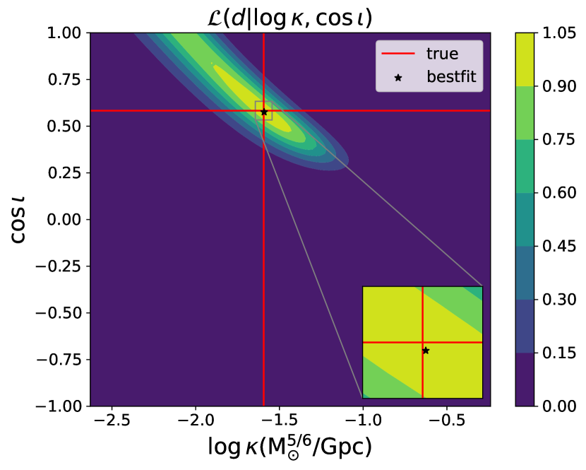
To avoid these two issues and mimic the realistic data analysis more closely, we choose to directly calculate the likelihood using Eq. (11): we sample the Gaussian noise using the power spectrum of each detector to obtain the detector strain . Using the approximation that the uncertainties of and are mainly due to their mutual correlation, while their correlations with other parameters are negligible, the evaluation of Eq. (19) is approximated as
| (20) |
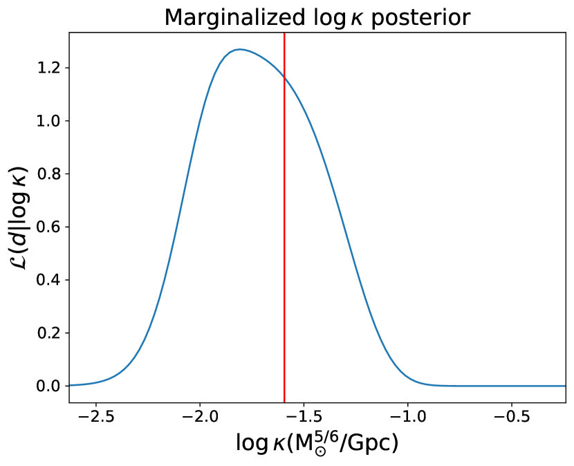
The Fisher matrix, however, is used to give a rough estimation of and range within which is calculated. For each event, we calculate the likelihood on linear grid of and , with a 3- range around the true parameter values. The uncertainties and are given by the Fisher approximation. Fig. 1 displays the likelihood for an example event, which clearly shows the strong degeneracy between and . The marginalized likelihood for the same event is shown in Fig. 2, which displays more features than the Gaussian likelihood given by the simple Fisher matrix approximation.
To summarize, the steps of inferring the BNS population model from a number of simulated BNS events are stated as follows: 1) generating of BNS events with total number , and parameters sampled from an injection population model ; 2) calculating the observed SNR of each event with Eq. (15), and labelling loud events with as detected; 3) picking a population model , constraining the population model and the total number of events in the framework of hierarchical Bayesian analysis with the population likelihood in Eq. (13), the evaluation of which makes use of the likelihood of individual events in Eq. (11). The implementation of these steps are coded in a Python package PoppinGW we developed, where GWFAST [75] is used in waveform related calculations and BILBY [76] is used for conducting Bayesian inferences. Source code of PoppinGW is available on GitHub \faGithub https://github.com/mzLi01/poppingw.
III.2 Examples of BNS population inference
In this subsection, we aim to examine how accurately the BNS population model and therefore the foreground energy density of BNSs can be constrained with the hierarchical Bayesian method from simulated BNS observations with 3G detectors.
As a fiducial population model, we use the same BNS merger rate model as in Paper I,
| (21) |
with the local merger rate [71, 72] (see e.g. [77, 58, 78] for more detailed rate modeling). The total merger rate in the observer frame is then
| (22) |
where is the comoving volume of the Universe within redshift . In the fiducial model, the total merger rate turns out to be . For other parameters, we set
| (23) | ||||
where are masses of the binary.
As a convenient example, we sample a total number of BNS events from the fiducial population model, events among these have SNR exceed the detection threshold, i.e., . We perform the population inference on these individually detected events.
Before implementing the Bayesian population inference with likelihood in Eq. (13), we need to determine the parameterization form of the population . To be as general as possible, we parameterize using cubic spline interpolation among a number of discrete points with . The boundary values and are fixed to be zero, considering the low probability of BNS mergers at extremely low and extremely high redshifts. In this general BNS population model with model parameters , the probability density of given is expressed as
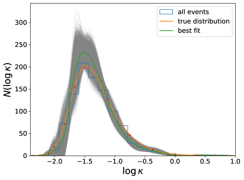
where is the cubic spline interpolation function with given control point values (see red dots in Fig. 3 for the control points) and we have applied normalization on the probability density function for arbitrary values of . This model is (almost) free of any assumption on the star formation rate and the delay time of BNS mergers thereafter, therefore the reconstructed BNS population is expected to be unbiased.
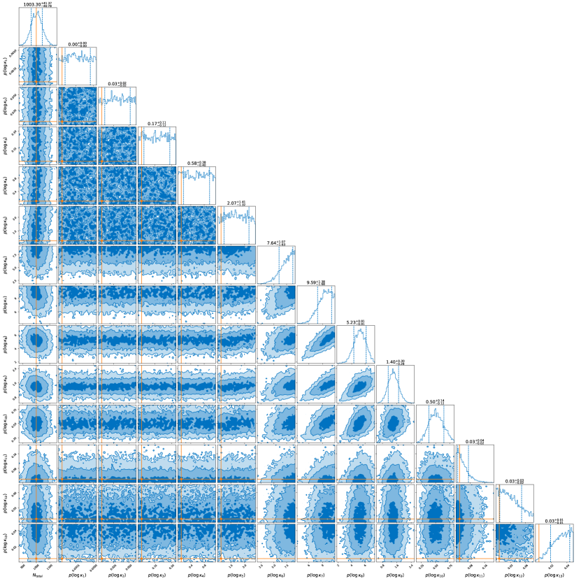
With this general population model, we constrain the population model parameters from the events. Fig. 3 displays the corner plot of the posterior contours, where the total number uncertainty is consistent with the Possion distribution with , and the constraints on at middle bins ( ) are highly correlated. Though this correlation seems biases the parameter constraints, the constraint on the number of events in each bin is well behaved as shown in Fig. 4.
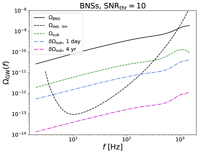
After the BNS population reconstructed, the energy density of the foreground from all the BNSs and subthreshold BNSs can be calculated using Eq. (5), where the selection effect is also taken into account in the latter calculations. We choose posterior samples from the constrained population model and calculate for each sample population. The uncertainty range is therefore estimated as . As shown in Fig. 5, in the fiducial population , which is measured with fractional uncertainty from day’s observations. The measurement precision would be largely improved with many more BNS events available in year long observations of 3G detectors, i.e.,
| (24) |
is expected, where we have used the fiducial merger rate [Eq. (22)] in the second equal sign.
For comparison, we also plot the detector sensitivity limit which is the sensitivity of the detector network to the SGWB if no astrophysical foreground presented. We adopt a commonly used definition, the power-law integrated sensitivity curve proposed in [79], assuming a threshold and an observation time of : any SGWB with energy density that is tangent to the detector sensitivity limit curve at , i.e.,
| (25) |
with the power index can be detected by the detector network with confidence level in 4 years (see [80, 58] for the computational details).
As shown in Fig. 5, the measurement uncertainty is below in the entire frequency range. Therefore the sensitivity for detecting the primordial SGWB is mainly limited by the detector noise level and the total observation time, and the foreground of BNSs after proper cleaning is a minor limiting factor.
IV Summary
Foreground cleaning is essential for detecting the SGWB. In a nutshell, foreground cleaning is to measure and subtract the foreground energy density or equivalently the PSD. There are in general two approaches in understanding and cleaning the foreground, an event-to-event approach in Eq. (4), and a population based approach in Eq. (5). In the 3G era, most of BBHs and a fraction of BNSs are expected to be loud enough and can be individually detected. Their contribution to the foreground can be cleaned with high precision using the event-to-event approach, as shown in Paper I. However, cleaning the foreground of subthreshold BNSs has been a long-standing open question, which we aim to solve in this work.
We propose that the foreground PSD of subthreshold BNSs can be measured with the population based approach. The basic idea is rather straightforward: the orientations of BNSs in the Universe should be isotropic, i.e., a uniform distribution in , therefore one can infer the number of subthreshold BNSs from individually detected ones and their contribution to the foreground PSD, i.e., . In practice, the idea above is conducted in the framework of Bayesian population analysis.
As a convenient example, we constrain the BNS population model from a small number () of BNS events sampled from an injection population . With the constrained population model shown in Fig. 4, we find the foreground energy density from subthreshold BNSs is measured with fractional uncertainty , where . With a much higher number of BNS mergers available during years of observations of 3G detectors, a percent level measurement of is expected (see Fig. 5).
As a result, the residual foreground energy density from either the loud events or the subthreshold events after the foregroud cleaning is expected to be below the detector sensitivity limit , therefore the astrophysical foregrounds from compact binaries will not be a limiting factor of the detection of the primordial SGWB with 3G detector network. Instead, it will be limited by the detector noise level and the total observation time, i.e., . Assuming the fiducial 3G detector network and a -yr observation, a flat SGWB with is expected to be detected at 3 confidence level (see Fig. 5).
The cleaning methods proposed in Paper I and in this work can be equally applied to black hole-neutron star (BH-NS) binaries, which are expected to contribute a minor component to the astrophysical foregrounds with due to the much lower merger rate [48]. After implementing the same cleaning, the residue foreground energy density of BH-NS binaries should be lower than that of BNSs, therefore is not likely a limiting factor for detecting the primordial SGWB either.
Acknowledgements.
We thank Bei Zhou for sharing the detector sensitivity limit curve. This work made use of the Gravity Supercomputer at the Department of Astronomy, Shanghai Jiao Tong University.References
- Guth [1981] A. H. Guth, Inflationary universe: A possible solution to the horizon and flatness problems, Phys. Rev. D 23, 347 (1981).
- Linde [1982] A. D. Linde, A new inflationary universe scenario: A possible solution of the horizon, flatness, homogeneity, isotropy and primordial monopole problems, Physics Letters B 108, 389 (1982).
- Allahverdi et al. [2010] R. Allahverdi, R. Brandenberger, F.-Y. Cyr-Racine, and A. Mazumdar, Reheating in Inflationary Cosmology: Theory and Applications, Annual Review of Nuclear and Particle Science 60, 27 (2010), arXiv:1001.2600 [hep-th] .
- Amin et al. [2015] M. A. Amin, M. P. Hertzberg, D. I. Kaiser, and J. Karouby, Nonperturbative dynamics of reheating after inflation: A review, International Journal of Modern Physics D 24, 1530003 (2015), arXiv:1410.3808 [hep-ph] .
- Turner and Wilczek [1990] M. S. Turner and F. Wilczek, Relic gravitational waves and extended inflation, Phys. Rev. Lett. 65, 3080 (1990).
- Turner et al. [1992] M. S. Turner, E. J. Weinberg, and L. M. Widrow, Bubble nucleation in first-order inflation and other cosmological phase transitions, Physical Review D 46, 2384 (1992).
- Kamionkowski et al. [1994] M. Kamionkowski, A. Kosowsky, and M. S. Turner, Gravitational radiation from first-order phase transitions, Phys. Rev. D 49, 2837 (1994).
- Kosowsky et al. [1992] A. Kosowsky, M. S. Turner, and R. Watkins, Gravitational radiation from colliding vacuum bubbles, Phys. Rev. D 45, 4514 (1992).
- Caprini et al. [2008] C. Caprini, R. Durrer, and G. Servant, Gravitational wave generation from bubble collisions in first-order phase transitions: An analytic approach, Phys. Rev. D 77, 124015 (2008).
- Cutting et al. [2018] D. Cutting, M. Hindmarsh, and D. J. Weir, Gravitational waves from vacuum first-order phase transitions: From the envelope to the lattice, Physical Review D 97, 123513 (2018), arXiv:1802.05712 [astro-ph.CO] .
- Vilenkin [1981] A. Vilenkin, Gravitational radiation from cosmic strings, Physics Letters B 107, 47 (1981).
- Hogan and Rees [1984] C. J. Hogan and M. J. Rees, Gravitational interactions of cosmic strings, Nature (London) 311, 109 (1984).
- Caldwell and Allen [1992] R. R. Caldwell and B. Allen, Cosmological constraints on cosmic-string gravitational radiation, Physical Review D 45, 3447 (1992).
- Hindmarsh and Kibble [1995] M. B. Hindmarsh and T. W. B. Kibble, Cosmic strings, Reports on Progress in Physics 58, 477 (1995), arXiv:hep-ph/9411342 [hep-ph] .
- Vilenkin and Shellard [2000] A. Vilenkin and E. P. S. Shellard, Cosmic Strings and Other Topological Defects (2000).
- Buchmüller et al. [2021] W. Buchmüller, V. Domcke, and K. Schmitz, Stochastic gravitational-wave background from metastable cosmic strings, JCAP 2021, 006 (2021), arXiv:2107.04578 [hep-ph] .
- Allen [1997] B. Allen, The Stochastic Gravity-Wave Background: Sources and Detection, in Relativistic Gravitation and Gravitational Radiation, edited by J.-A. Marck and J.-P. Lasota (1997) pp. 373–417, arXiv:gr-qc/9604033 [gr-qc] .
- Chiara Guzzetti et al. [2016] M. Chiara Guzzetti, N. Bartolo, M. Liguori, and S. Matarrese, Gravitational waves from inflation, arXiv e-prints , arXiv:1605.01615 (2016), arXiv:1605.01615 [astro-ph.CO] .
- Cai et al. [2017] R.-G. Cai, Z. Cao, Z.-K. Guo, S.-J. Wang, and T. Yang, The Gravitational-Wave Physics, National Science Review 4, 687 (2017), arXiv:1703.00187 [gr-qc] .
- Caprini and Figueroa [2018] C. Caprini and D. G. Figueroa, Cosmological backgrounds of gravitational waves, Classical and Quantum Gravity 35, 163001 (2018), arXiv:1801.04268 [astro-ph.CO] .
- Christensen [2019] N. Christensen, Stochastic gravitational wave backgrounds, Reports on Progress in Physics 82, 016903 (2019), arXiv:1811.08797 [gr-qc] .
- Renzini et al. [2022] A. I. Renzini, B. Goncharov, A. C. Jenkins, and P. M. Meyers, Stochastic Gravitational-Wave Backgrounds: Current Detection Efforts and Future Prospects, Galaxies 10, 34 (2022), arXiv:2202.00178 [gr-qc] .
- Hobbs et al. [2010] G. Hobbs, A. Archibald, Z. Arzoumanian, D. Backer, M. Bailes, N. D. R. Bhat, M. Burgay, S. Burke-Spolaor, D. Champion, I. Cognard, W. Coles, J. Cordes, P. Demorest, G. Desvignes, R. D. Ferdman, L. Finn, P. Freire, M. Gonzalez, J. Hessels, A. Hotan, G. Janssen, F. Jenet, A. Jessner, C. Jordan, V. Kaspi, M. Kramer, V. Kondratiev, J. Lazio, K. Lazaridis, K. J. Lee, Y. Levin, A. Lommen, D. Lorimer, R. Lynch, A. Lyne, R. Manchester, M. McLaughlin, D. Nice, S. Oslowski, M. Pilia, A. Possenti, M. Purver, S. Ransom, J. Reynolds, S. Sanidas, J. Sarkissian, A. Sesana, R. Shannon, X. Siemens, I. Stairs, B. Stappers, D. Stinebring, G. Theureau, R. van Haasteren, W. van Straten, J. P. W. Verbiest, D. R. B. Yardley, and X. P. You, The International Pulsar Timing Array project: using pulsars as a gravitational wave detector, Classical and Quantum Gravity 27, 084013 (2010), arXiv:0911.5206 [astro-ph.SR] .
- McLaughlin [2013] M. A. McLaughlin, The North American Nanohertz Observatory for Gravitational Waves, Classical and Quantum Gravity 30, 224008 (2013), arXiv:1310.0758 [astro-ph.IM] .
- Hobbs [2013] G. Hobbs, The Parkes Pulsar Timing Array, Classical and Quantum Gravity 30, 224007 (2013), arXiv:1307.2629 [astro-ph.IM] .
- Lentati et al. [2015] L. Lentati, S. R. Taylor, C. M. F. Mingarelli, A. Sesana, S. A. Sanidas, A. Vecchio, R. N. Caballero, K. J. Lee, R. van Haasteren, S. Babak, C. G. Bassa, P. Brem, M. Burgay, D. J. Champion, I. Cognard, G. Desvignes, J. R. Gair, L. Guillemot, J. W. T. Hessels, G. H. Janssen, R. Karuppusamy, M. Kramer, A. Lassus, P. Lazarus, K. Liu, S. Osłowski, D. Perrodin, A. Petiteau, A. Possenti, M. B. Purver, P. A. Rosado, R. Smits, B. Stappers, G. Theureau, C. Tiburzi, and J. P. W. Verbiest, European Pulsar Timing Array limits on an isotropic stochastic gravitational-wave background, MNRAS 453, 2576 (2015), arXiv:1504.03692 [astro-ph.CO] .
- Thorpe et al. [2019] J. I. Thorpe, J. Ziemer, I. Thorpe, J. Livas, J. W. Conklin, R. Caldwell, E. Berti, S. T. McWilliams, R. Stebbins, D. Shoemaker, E. C. Ferrara, S. L. Larson, D. Shoemaker, J. S. Key, M. Vallisneri, M. Eracleous, J. Schnittman, B. Kamai, J. Camp, G. Mueller, J. Bellovary, N. Rioux, J. Baker, P. L. Bender, C. Cutler, N. Cornish, C. Hogan, S. Manthripragada, B. Ware, P. Natarajan, K. Numata, S. R. Sankar, B. J. Kelly, K. McKenzie, J. Slutsky, R. Spero, M. Hewitson, S. Francis, R. DeRosa, A. Yu, A. Hornschemeier, and P. Wass, The Laser Interferometer Space Antenna: Unveiling the Millihertz Gravitational Wave Sky, in Bulletin of the American Astronomical Society, Vol. 51 (2019) p. 77, arXiv:1907.06482 [astro-ph.IM] .
- Mei et al. [2021] J. Mei, Y.-Z. Bai, J. Bao, E. Barausse, L. Cai, E. Canuto, B. Cao, W.-M. Chen, Y. Chen, Y.-W. Ding, H.-Z. Duan, H. Fan, W.-F. Feng, H. Fu, Q. Gao, T. Gao, Y. Gong, X. Gou, C.-Z. Gu, D.-F. Gu, Z.-Q. He, M. Hendry, W. Hong, X.-C. Hu, Y.-M. Hu, Y. Hu, S.-J. Huang, X.-Q. Huang, Q. Jiang, Y.-Z. Jiang, Y. Jiang, Z. Jiang, H.-M. Jin, V. Korol, H.-Y. Li, M. Li, M. Li, P. Li, R. Li, Y. Li, Z. Li, Z. Li, Z.-X. Li, Y.-R. Liang, Z.-C. Liang, F.-J. Liao, Q. Liu, S. Liu, Y.-C. Liu, L. Liu, P.-B. Liu, X. Liu, Y. Liu, X.-F. Lu, Y. Lu, Z.-H. Lu, Y. Luo, Z.-C. Luo, V. Milyukov, M. Ming, X. Pi, C. Qin, S.-B. Qu, A. Sesana, C. Shao, C. Shi, W. Su, D.-Y. Tan, Y. Tan, Z. Tan, L.-C. Tu, B. Wang, C.-R. Wang, F. Wang, G.-F. Wang, H. Wang, J. Wang, L. Wang, P. Wang, X. Wang, Y. Wang, Y.-F. Wang, R. Wei, S.-C. Wu, C.-Y. Xiao, X.-S. Xu, C. Xue, F.-C. Yang, L. Yang, M.-L. Yang, S.-Q. Yang, B. Ye, H.-C. Yeh, S. Yu, D. Zhai, C. Zhang, H. Zhang, J.-d. Zhang, J. Zhang, L. Zhang, X. Zhang, X. Zhang, H. Zhou, M.-Y. Zhou, Z.-B. Zhou, D.-D. Zhu, T.-G. Zi, and J. Luo, The TianQin project: Current progress on science and technology, Progress of Theoretical and Experimental Physics 2021, 05A107 (2021), arXiv:2008.10332 [gr-qc] .
- Collaboration [2015] L. S. Collaboration, Advanced LIGO, Classical and Quantum Gravity 32, 074001 (2015), arXiv:1411.4547 [gr-qc] .
- Acernese et al. [2015] F. Acernese, M. Agathos, K. Agatsuma, D. Aisa, N. Allemandou, A. Allocca, J. Amarni, P. Astone, G. Balestri, G. Ballardin, F. Barone, J. P. Baronick, M. Barsuglia, A. Basti, F. Basti, T. S. Bauer, V. Bavigadda, M. Bejger, M. G. Beker, C. Belczynski, D. Bersanetti, A. Bertolini, M. Bitossi, M. A. Bizouard, S. Bloemen, M. Blom, M. Boer, G. Bogaert, D. Bondi, F. Bondu, L. Bonelli, R. Bonnand, V. Boschi, L. Bosi, T. Bouedo, C. Bradaschia, M. Branchesi, T. Briant, A. Brillet, V. Brisson, T. Bulik, H. J. Bulten, D. Buskulic, C. Buy, G. Cagnoli, E. Calloni, C. Campeggi, B. Canuel, F. Carbognani, F. Cavalier, R. Cavalieri, G. Cella, E. Cesarini, E. C. Mottin, A. Chincarini, A. Chiummo, S. Chua, F. Cleva, E. Coccia, P. F. Cohadon, A. Colla, M. Colombini, A. Conte, J. P. Coulon, E. Cuoco, A. Dalmaz, S. D’Antonio, V. Dattilo, M. Davier, R. Day, G. Debreczeni, J. Degallaix, S. Deléglise, W. D. Pozzo, H. Dereli, R. D. Rosa, L. D. Fiore, A. D. Lieto, A. D. Virgilio, M. Doets, V. Dolique, M. Drago, M. Ducrot, G. Endrőczi, V. Fafone, S. Farinon, I. Ferrante, F. Ferrini, F. Fidecaro, I. Fiori, R. Flaminio, J. D. Fournier, S. Franco, S. Frasca, F. Frasconi, L. Gammaitoni, F. Garufi, M. Gaspard, A. Gatto, G. Gemme, B. Gendre, E. Genin, A. Gennai, S. Ghosh, L. Giacobone, A. Giazotto, R. Gouaty, M. Granata, G. Greco, P. Groot, G. M. Guidi, J. Harms, A. Heidmann, H. Heitmann, P. Hello, G. Hemming, E. Hennes, D. Hofman, P. Jaranowski, R. J. G. Jonker, M. Kasprzack, F. Kéfélian, I. Kowalska, M. Kraan, A. Królak, A. Kutynia, C. Lazzaro, M. Leonardi, N. Leroy, N. Letendre, T. G. F. Li, B. Lieunard, M. Lorenzini, V. Loriette, G. Losurdo, C. Magazzù, E. Majorana, I. Maksimovic, V. Malvezzi, N. Man, V. Mangano, M. Mantovani, F. Marchesoni, F. Marion, J. Marque, F. Martelli, L. Martellini, A. Masserot, D. Meacher, J. Meidam, F. Mezzani, C. Michel, L. Milano, Y. Minenkov, A. Moggi, M. Mohan, M. Montani, N. Morgado, B. Mours, F. Mul, M. F. Nagy, I. Nardecchia, L. Naticchioni, G. Nelemans, I. Neri, M. Neri, F. Nocera, E. Pacaud, C. Palomba, F. Paoletti, A. Paoli, A. Pasqualetti, R. Passaquieti, D. Passuello, M. Perciballi, S. Petit, M. Pichot, F. Piergiovanni, G. Pillant, A. Piluso, L. Pinard, R. Poggiani, M. Prijatelj, G. A. Prodi, M. Punturo, P. Puppo, D. S. Rabeling, I. Rácz, P. Rapagnani, M. Razzano, V. Re, T. Regimbau, F. Ricci, F. Robinet, A. Rocchi, L. Rolland, R. Romano, D. Rosińska, P. Ruggi, E. Saracco, B. Sassolas, F. Schimmel, D. Sentenac, V. Sequino, S. Shah, K. Siellez, N. Straniero, B. Swinkels, M. Tacca, M. Tonelli, F. Travasso, M. Turconi, G. Vajente, N. van Bakel, M. van Beuzekom, J. F. J. van den Brand, C. Van Den Broeck, M. V. van der Sluys, J. van Heijningen, M. Vasúth, G. Vedovato, J. Veitch, D. Verkindt, F. Vetrano, A. Viceré, J. Y. Vinet, G. Visser, H. Vocca, R. Ward, M. Was, L. W. Wei, M. Yvert, A. Z. żny, and J. P. Zendri, Advanced Virgo: a second-generation interferometric gravitational wave detector, Classical and Quantum Gravity 32, 024001 (2015), arXiv:1408.3978 [gr-qc] .
- Aso et al. [2013] Y. Aso, Y. Michimura, K. Somiya, M. Ando, O. Miyakawa, T. Sekiguchi, D. Tatsumi, and H. Yamamoto (The KAGRA Collaboration), Interferometer design of the kagra gravitational wave detector, Phys. Rev. D 88, 043007 (2013).
- Agazie et al. [2023a] G. Agazie et al. (NANOGrav), The NANOGrav 15 yr Data Set: Evidence for a Gravitational-wave Background, Astrophys. J. Lett. 951, L8 (2023a), arXiv:2306.16213 [astro-ph.HE] .
- Agazie et al. [2023b] G. Agazie et al. (NANOGrav), The NANOGrav 15 yr Data Set: Observations and Timing of 68 Millisecond Pulsars, Astrophys. J. Lett. 951, L9 (2023b), arXiv:2306.16217 [astro-ph.HE] .
- Collaboration et al. [2023] T. I. P. T. A. Collaboration, G. Agazie, J. Antoniadis, A. Anumarlapudi, A. M. Archibald, P. Arumugam, S. Arumugam, Z. Arzoumanian, J. Askew, S. Babak, M. Bagchi, M. Bailes, A.-S. B. Nielsen, P. T. Baker, C. G. Bassa, et al., Comparing recent PTA results on the nanohertz stochastic gravitational wave background (2023), arxiv:2309.00693 [astro-ph, physics:gr-qc] .
- Reardon et al. [2023] D. J. Reardon et al., Search for an Isotropic Gravitational-wave Background with the Parkes Pulsar Timing Array, Astrophys. J. Lett. 951, L6 (2023), arXiv:2306.16215 [astro-ph.HE] .
- Zic et al. [2023] A. Zic et al., The Parkes Pulsar Timing Array third data release, Publ. Astron. Soc. Austral. 40, e049 (2023), arXiv:2306.16230 [astro-ph.HE] .
- Antoniadis et al. [2023a] J. Antoniadis et al. (EPTA), The second data release from the European Pulsar Timing Array III. Search for gravitational wave signals, Astron. Astrophys. 678, A50 (2023a), arXiv:2306.16214 [astro-ph.HE] .
- Antoniadis et al. [2023b] J. Antoniadis et al. (EPTA), The second data release from the European Pulsar Timing Array I. The dataset and timing analysis, Astron. Astrophys. 678, A48 (2023b), arXiv:2306.16224 [astro-ph.HE] .
- Xu et al. [2023] H. Xu et al., Searching for the Nano-Hertz Stochastic Gravitational Wave Background with the Chinese Pulsar Timing Array Data Release I, Res. Astron. Astrophys. 23, 075024 (2023), arXiv:2306.16216 [astro-ph.HE] .
- Afzal et al. [2023] A. Afzal et al. (NANOGrav), The NANOGrav 15 yr Data Set: Search for Signals from New Physics, Astrophys. J. Lett. 951, L11 (2023), arXiv:2306.16219 [astro-ph.HE] .
- Antoniadis et al. [2023c] J. Antoniadis, P. Arumugam, S. Arumugam, P. Auclair, S. Babak, M. Bagchi, A.-S. B. Nielsen, E. Barausse, C. G. Bassa, A. Bathula, A. Berthereau, M. Bonetti, E. Bortolas, P. R. Brook, M. Burgay, et al., The second data release from the European Pulsar Timing Array: V. Implications for massive black holes, dark matter and the early Universe (2023c), arxiv:2306.16227 [astro-ph, physics:gr-qc] .
- Agazie et al. [2023c] G. Agazie et al. (NANOGrav), The NANOGrav 15 yr Data Set: Constraints on Supermassive Black Hole Binaries from the Gravitational-wave Background, Astrophys. J. Lett. 952, L37 (2023c), arXiv:2306.16220 [astro-ph.HE] .
- Agazie et al. [2023d] G. Agazie et al. (NANOGrav), The NANOGrav 15 yr Data Set: Bayesian Limits on Gravitational Waves from Individual Supermassive Black Hole Binaries, Astrophys. J. Lett. 951, L50 (2023d), arXiv:2306.16222 [astro-ph.HE] .
- Bi et al. [2023] Y.-C. Bi, Y.-M. Wu, Z.-C. Chen, and Q.-G. Huang, Implications for the supermassive black hole binaries from the NANOGrav 15-year data set, Sci. China Phys. Mech. Astron. 66, 120402 (2023), arXiv:2307.00722 [astro-ph.CO] .
- Regimbau et al. [2017] T. Regimbau, M. Evans, N. Christensen, E. Katsavounidis, B. Sathyaprakash, and S. Vitale, Digging Deeper: Observing Primordial Gravitational Waves below the Binary-Black-Hole-Produced Stochastic Background, Phys. Rev. Lett. 118, 151105 (2017), arXiv:1611.08943 [astro-ph.CO] .
- ET0 [2018] ET-0000A-18, https://apps.et-gw.eu/tds/?content=3&r=14065 (2018).
- Srivastava et al. [2022] V. Srivastava, D. Davis, K. Kuns, P. Landry, S. Ballmer, M. Evans, E. D. Hall, J. Read, and B. S. Sathyaprakash, Science-driven Tunable Design of Cosmic Explorer Detectors, The Astrophysical Journal 931, 22 (2022), arXiv:2201.10668 [gr-qc] .
- Branchesi et al. [2023] M. Branchesi, M. Maggiore, D. Alonso, C. Badger, B. Banerjee, F. Beirnaert, E. Belgacem, S. Bhagwat, G. Boileau, S. Borhanian, D. D. Brown, M. Leong Chan, G. Cusin, S. L. Danilishin, J. Degallaix, V. De Luca, A. Dhani, T. Dietrich, U. Dupletsa, S. Foffa, G. Franciolini, A. Freise, G. Gemme, B. Goncharov, A. Ghosh, F. Gulminelli, I. Gupta, P. Kumar Gupta, J. Harms, N. Hazra, S. Hild, T. Hinderer, I. Siong Heng, F. Iacovelli, J. Janquart, K. Janssens, A. C. Jenkins, C. Kalaghatgi, X. Koroveshi, T. G. F. Li, Y. Li, E. Loffredo, E. Maggio, M. Mancarella, M. Mapelli, K. Martinovic, A. Maselli, P. Meyers, A. L. Miller, C. Mondal, N. Muttoni, H. Narola, M. Oertel, G. Oganesyan, C. Pacilio, C. Palomba, P. Pani, A. Pasqualetti, A. Perego, C. Périgois, M. Pieroni, O. J. Piccinni, A. Puecher, P. Puppo, A. Ricciardone, A. Riotto, S. Ronchini, M. Sakellariadou, A. Samajdar, F. Santoliquido, B. S. Sathyaprakash, J. Steinlechner, S. Steinlechner, A. Utina, C. Van Den Broeck, and T. Zhang, Science with the Einstein Telescope: a comparison of different designs, JCAP 2023, 068 (2023), arXiv:2303.15923 [gr-qc] .
- Drasco and Flanagan [2003] S. Drasco and É. É. Flanagan, Detection methods for non-Gaussian gravitational wave stochastic backgrounds, Physical Review D 67, 082003 (2003), arXiv:gr-qc/0210032 [gr-qc] .
- Smith and Thrane [2018] R. Smith and E. Thrane, Optimal search for an astrophysical gravitational-wave background, Phys. Rev. X 8, 021019 (2018).
- Biscoveanu et al. [2020] S. Biscoveanu, C. Talbot, E. Thrane, and R. Smith, Measuring the primordial gravitational-wave background in the presence of astrophysical foregrounds, Phys. Rev. Lett. 125, 241101 (2020).
- Zhong et al. [2022] H. Zhong, R. Ormiston, and V. Mandic, Detecting cosmological gravitational waves background after removal of compact binary coalescences in future gravitational wave detectors, arXiv e-prints , arXiv:2209.11877 (2022), arXiv:2209.11877 [gr-qc] .
- Sharma and Harms [2020] A. Sharma and J. Harms, Searching for cosmological gravitational-wave backgrounds with third-generation detectors in the presence of an astrophysical foreground, Physical Review D 102, 063009 (2020), arXiv:2006.16116 [gr-qc] .
- Pan and Yang [2023] Z. Pan and H. Yang, Improving the detection sensitivity to primordial stochastic gravitational waves with reduced astrophysical foregrounds, Physical Review D 107, 123036 (2023), arXiv:2301.04529 [gr-qc] .
- Cutler and Harms [2006] C. Cutler and J. Harms, Big Bang Observer and the neutron-star-binary subtraction problem, Physical Review D 73, 042001 (2006), arXiv:gr-qc/0511092 [gr-qc] .
- Harms et al. [2008] J. Harms, C. Mahrdt, M. Otto, and M. Prieß, Subtraction-noise projection in gravitational-wave detector networks, Physical Review D 77, 123010 (2008), arXiv:0803.0226 [gr-qc] .
- Sachdev et al. [2020] S. Sachdev, T. Regimbau, and B. S. Sathyaprakash, Subtracting compact binary foreground sources to reveal primordial gravitational-wave backgrounds, Physical Review D 102, 024051 (2020), arXiv:2002.05365 [gr-qc] .
- Zhou et al. [2022a] B. Zhou, L. Reali, E. Berti, M. Çalışkan, C. Creque-Sarbinowski, M. Kamionkowski, and B. S. Sathyaprakash, Subtracting Compact Binary Foregrounds to Search for Subdominant Gravitational-Wave Backgrounds in Next-Generation Ground-Based Observatories, arXiv e-prints , arXiv:2209.01310 (2022a), arXiv:2209.01310 [gr-qc] .
- Zhou et al. [2022b] B. Zhou, L. Reali, E. Berti, M. Çalışkan, C. Creque-Sarbinowski, M. Kamionkowski, and B. S. Sathyaprakash, Compact Binary Foreground Subtraction in Next-Generation Ground-Based Observatories, arXiv e-prints , arXiv:2209.01221 (2022b), arXiv:2209.01221 [gr-qc] .
- Song et al. [2024] H. Song, D. Liang, Z. Wang, and L. Shao, Compact Binary Foreground Subtraction for Detecting the Stochastic Gravitational-wave Background in Ground-based Detectors, arXiv e-prints , arXiv:2401.00984 (2024), arXiv:2401.00984 [gr-qc] .
- Pan and Yang [2020] Z. Pan and H. Yang, Probing Primordial Stochastic Gravitational Wave Background with Multi-band Astrophysical Foreground Cleaning, Class. Quant. Grav. 37, 195020 (2020), arXiv:1910.09637 [astro-ph.CO] .
- Planck Collaboration et al. [2020] Planck Collaboration, N. Aghanim, Y. Akrami, M. Ashdown, J. Aumont, C. Baccigalupi, M. Ballardini, A. J. Banday, R. B. Barreiro, N. Bartolo, S. Basak, R. Battye, K. Benabed, J. P. Bernard, M. Bersanelli, et al., Planck 2018 results. VI. Cosmological parameters, Astronomy and Astrophysics 641, A6 (2020).
- Allen and Romano [1999] B. Allen and J. D. Romano, Detecting a stochastic background of gravitational radiation: Signal processing strategies and sensitivities, Physical Review D 59, 102001 (1999), arXiv:gr-qc/9710117 [gr-qc] .
- Phinney [2001] E. S. Phinney, A Practical Theorem on Gravitational Wave Backgrounds, arXiv e-prints , astro-ph/0108028 (2001), arXiv:astro-ph/0108028 [astro-ph] .
- Pan and Yang [2020] Z. Pan and H. Yang, Probing primordial stochastic gravitational wave background with multi-band astrophysical foreground cleaning, Classical and Quantum Gravity 37, 195020 (2020), arXiv:1910.09637 [astro-ph.CO] .
- Sathyaprakash and Schutz [2009] B. S. Sathyaprakash and B. F. Schutz, Physics, Astrophysics and Cosmology with Gravitational Waves, Living Reviews in Relativity 12, 2 (2009), arXiv:0903.0338 [gr-qc] .
- Husa et al. [2016] S. Husa, S. Khan, M. Hannam, M. Pürrer, F. Ohme, X. J. Forteza, and A. Bohé, Frequency-domain gravitational waves from non-precessing black-hole binaries. I. New numerical waveforms and anatomy of the signal, Physical Review D 93, 044006 (2016), arxiv:1508.07250 [gr-qc] .
- Khan et al. [2016] S. Khan, S. Husa, M. Hannam, F. Ohme, M. Pürrer, X. J. Forteza, and A. Bohé, Frequency-domain gravitational waves from non-precessing black-hole binaries. II. A phenomenological model for the advanced detector era, Physical Review D 93, 044007 (2016), arxiv:1508.07253 [gr-qc] .
- Abbott et al. [2021] R. Abbott, T. D. Abbott, S. Abraham, F. Acernese, K. Ackley, A. Adams, C. Adams, R. X. Adhikari, V. B. Adya, C. Affeldt, M. Agathos, K. Agatsuma, N. Aggarwal, O. D. Aguiar, L. Aiello, et al., GWTC-2: Compact Binary Coalescences Observed by LIGO and Virgo During the First Half of the Third Observing Run, Physical Review X 11, 021053 (2021), arxiv:2010.14527 [astro-ph, physics:gr-qc] .
- Borhanian [2021] S. Borhanian, GWBENCH: a novel Fisher information package for gravitational-wave benchmarking, Classical and Quantum Gravity 38, 175014 (2021), arXiv:2010.15202 [gr-qc] .
- LIGO Scientific Collaboration and Virgo Collaboration [2019] LIGO Scientific Collaboration and Virgo Collaboration, Binary Black Hole Population Properties Inferred from the First and Second Observing Runs of Advanced LIGO and Advanced Virgo, Astrophys.J.Lett. 882, L24 (2019), arXiv:1811.12940 [astro-ph.HE] .
- The LIGO Scientific Collaboration et al. [2021] The LIGO Scientific Collaboration, the Virgo Collaboration, and the KAGRA Collaboration, The population of merging compact binaries inferred using gravitational waves through GWTC-3, arXiv e-prints , arXiv:2111.03634 (2021), arXiv:2111.03634 [astro-ph.HE] .
- Gray et al. [2020] R. Gray, I. M. Hernandez, H. Qi, A. Sur, P. R. Brady, H.-Y. Chen, W. M. Farr, M. Fishbach, J. R. Gair, A. Ghosh, D. E. Holz, S. Mastrogiovanni, C. Messenger, D. A. Steer, J. Veitch, et al., Cosmological inference using gravitational wave standard sirens: A mock data analysis, Physical Review D 101, 122001 (2020).
- Vallisneri [2008] M. Vallisneri, Use and abuse of the Fisher information matrix in the assessment of gravitational-wave parameter-estimation prospects, Physical Review D 77, 042001 (2008).
- Iacovelli et al. [2022] F. Iacovelli, M. Mancarella, S. Foffa, and M. Maggiore, GWFAST: A Fisher information matrix Python code for third-generation gravitational-wave detectors, The Astrophysical Journal Supplement Series 263, 2 (2022), arxiv:2207.06910 [astro-ph, physics:gr-qc] .
- Ashton et al. [2019] G. Ashton, M. Hübner, P. D. Lasky, C. Talbot, K. Ackley, S. Biscoveanu, Q. Chu, A. Divakarla, P. J. Easter, B. Goncharov, F. Hernandez Vivanco, J. Harms, M. E. Lower, G. D. Meadors, D. Melchor, E. Payne, M. D. Pitkin, J. Powell, N. Sarin, R. J. E. Smith, and E. Thrane, BILBY: A User-friendly Bayesian Inference Library for Gravitational-wave Astronomy, The Astrophysical Journal Supplement Series 241, 27 (2019).
- Périgois et al. [2021] C. Périgois, C. Belczynski, T. Bulik, and T. Regimbau, startrack predictions of the stochastic gravitational-wave background from compact binary mergers, Phys. Rev. D 103, 043002 (2021).
- Regimbau [2022] T. Regimbau, The Quest for the Astrophysical Gravitational-Wave Background with Terrestrial Detectors, Symmetry 14, 270 (2022).
- Thrane and Romano [2013] E. Thrane and J. D. Romano, Sensitivity curves for searches for gravitational-wave backgrounds, Physical Review D 88, 124032 (2013), arXiv:1310.5300 [astro-ph.IM] .
- Moore et al. [2014] C. J. Moore, R. H. Cole, and C. P. L. Berry, Gravitational-wave sensitivity curves, Classical and Quantum Gravity 32, 015014 (2014).