Tsallis Entropy Regularization for Linearly Solvable MDP and Linear Quadratic Regulator
Yota Hashizume1, Koshi Oishi1 and Kenji Kashima1, Senior Member, IEEE1Y. Hashizume, K. Oishi, and K. Kashima are with the Graduate School of Informatics,
Kyoto University, Kyoto, Japan.
hashizume.yota.88n@st.kyoto-u.ac.jp; oishi.koshi.34y@st.kyoto-u.ac.jp; kk@i.kyoto-u.ac.jp This work
was supported by JSPS KAKENHI Grant Number JP21H04875.
Abstract
Shannon entropy regularization is widely adopted in optimal control due to its ability to promote exploration and enhance robustness, e.g., maximum entropy reinforcement learning known as Soft Actor-Critic.
In this paper, Tsallis entropy, which is a one-parameter extension of Shannon entropy, is used for the regularization of linearly solvable MDP and linear quadratic regulators.
We derive the solution for these problems and demonstrate its usefulness in balancing between exploration and sparsity of the obtained control law.
I Introduction
The incorporation of Shannon entropy of a control policy into the objective function of reinforcement learning, a technique known as maximum entropy reinforcement learning, has been applied in approaches like Soft Actor-Critic [1]. This method finds practical applications in various real-world scenarios, notably in fields like robotics.
An important feature of using entropy regularization is that the optimal policy is stochastic which is advantageous for exploration and
improves robustness [2].
Given these practical benefits, there is extensive research on optimal control utilizing entropy regularization.
When using entropy regularization,
the probability density function of the optimal control policy takes positive values for all input values.
Due to this property, entropy regularization cannot be applied to problems that require sparse control policies.
For example, in optimizing transportation routes for logistics,
a robust control policy is required to handle unforeseen circumstances such as disasters and traffic congestion [3].
However, since the number of available trucks is limited,
the number of routes is restricted, and the transportation plan needs to be sparse.
For such problems, while the robustness provided by entropy regularization is beneficial,
it does not satisfy the requirement for sparsity.
In [4], Tsallis entropy,
which originates from Tsallis statistical mechanics [5], is used to regularize optimal transport problems to obtain high-entropy, but sparse solutions.
In the context of reinforcement learning, [6, 7] have proposed a method
to obtain sparse control policies using a special case of Tsallis entropy.
In this study, we formulate a Tsallis entropy regularized optimal control problem (TROC)
for discrete-time systems and derive its Bellman equation.
The Bellman equations in [6, 7]
correspond to those with the deformation parameter set to .
In a general setting, finding the optimal control policy
using the derived Bellman equation is challenging due to the properties of Tsallis entropy.
In particular, we investigate the optimal control policies for linearly solvable Markov decision processes,
which correspond to optimal control on networks, and for the linear quadratic regulator, under the framework of TROC.
Through numerical examples, we verify that the optimal control policies achieve
high entropy while maintaining sparsity, demonstrating the usefulness of TROC.
The rest of the paper is organized as follows.
In Section II,
we describe the definitions and fundamental properties related to Tsallis entropy and Tsallis statistics.
In Section III, we formulate the TROC and derive its Bellman equation.
In Sections IV and V, based on the results from Section III,
we derive the optimal control policies for TROC applied to linearly solvable Markov decision processes
and linear quadratic regulators, respectively.
In Section VI, we briefly discuss the optimal transport problem.
Section VII concludes the paper.
Notation
Let and denote the expected value and variance of a random variable, respectively.
When the distinction between a random variable and its realization is not clear,
the random variable is denoted by , and its realization by .
Let denote the support of the probability density function , that is, the set . The Gamma function is denoted by .
II Preliminary: Tsallis entropy
In the context of Tsallis statistical mechanics[5], -exponential
functions, -products, and -sums are defined as one-parameter extensions of
the usual exponential functions, products, and sums, where is called a
deformation parameter
[8, 9, 10].
In the limit , they coincide with the usual ones. For simplicity, we assume in this paper.
Definition 1 (-Exponential and -Logarithm functions)
(1)
(2)
where .
Remark 1
The inverse function relationship exists, i.e.,
(3)
(4)
However, the standard exponent rules do not hold:
(5)
(6)
although -product can attain a similar formula [11].
Next, we define Tsallis entropy, which is a generalization of Shannon entropy
[9]. It converges to Shannon entropy in the limit
.
Definition 2
Tsallis entropy is defined as
(7)
The deformed -entropy defined below is used as a regularization term in [4].
It is related to the Tsallis entropy by the following relationship, which is referred
to as an additive duality.
Proposition 1 (-Entropy)
The deformed -entropy defined as
(8)
satisfies
(9)
This proposition indicates that the Tsallis entropy and deformed -entropy are
equivalent. In this study, we will use the deformed -entropy as a regularization
term for the sake of notational simplicity.
The KL divergence and Gaussian distribution are extended as follows [12, 13]:
Definition 3 (-KL Divergence)
The -KL divergence between density functions and is defined
as
(10)
The -KL divergence possesses some properties of the KL divergence, such as
non-negativity and convexity [12].
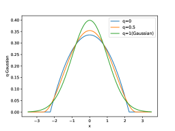
Definition 4 (multivariate -Gaussian)
A -Gaussian is an -dimensional random variable whose density function is given by
It follows from (1) that the support of the -Gaussian is bounded, represented as
(12)
This implies the closer is to , the smaller the support becomes.
See Fig. 1 for the density functions of -Gaussian as
varies.
III Tsallis Entropy Regularized Optimal Control Problem
III-AProblem formulation
Consider a discrete-time system with the state and the control input .
Conditional state transition probability distribution of under
, is denoted as . Also, denotes the
initial distribution. Under this setting, we formulate Tsallis Entropy Regularized
Optimal Control Problem (TROC).
Problem 1 (TROC)
Let the terminal time be . Find
the stochastic state feedback control policy , that minimizes the
cost function given by
(13)
where and is the conditioned deformed -entropy
(14)
The objective of Problem 1 is to balance the traditional cost minimization
(i.e., the sum of running costs and the terminal cost
) and the maximization of the deformed -entropy of the control
policy, which encourages exploration in the control policy. The parameter controls the trade-off between
these objectives.
III-BBellman equation for TROC
In this section, we derive the Bellman equation for TROC in a general setting.
The state-value function is introduced as
(15)
and state-input value function
(16)
Then, we obtain the following:
Theorem 1 (Bellman Equation for TROC)
For Problem 1, the optimal control policy is given by
(17)
where is determined by .
The value function in (15) is the solution to
(18)
(19)
Proof:
Standard dynamic programming yields
(20)
By Lemma 1 in the Appendix, the minimizer of (20) is given by (17).
Substituting this into (20) yields (18).
∎
In the case of the Shannon entropy regularized optimal control problem [15], that is,
when , the Bellman equation (18) is replaced by
(21)
and . Moreover, the optimal control policy is given by the soft-max function
(22)
which is positive for all .
On the contrary, in the case of TROC, the distribution in (17),
which is called ent-max [16], does not satisfy . In fact, the support of ent-max function is bounded.
IV -Kullback-Leibler control
IV-ALinearly solvable Markov Decision Processes
Kullback-Leibler (KL) control is a control problem having costs described in terms of the KL divergence, enabling efficient numerical solutions to nonlinear optimal
control problems [17]. Since KL control can also be interpreted as an entropy-regularized
optimal control problem, it can be extended to the Tsallis entropy framework by
replacing KL divergence with -KL divergence.
In this section, we assume states are defined on a finite set , and control inputs are given by a transition matrix
. That is, if at time , the state is distributed
according to the probability vector , then at time ,
the state distributes according to with input .
Under this setting, we formulate the -KL control problem as follows:
Problem 2 (-KL Control Problem)
Consider a Markov process
with transition matrix . For the initial distribution
, state stage cost , transition matrix ,
terminal time , and , find the transition
matrices that minimize the cost function
given by
(23)
Here, is the -KL divergence in the discrete case, defined as
(24)
According to the objective function (23),
the goal of Problem 2 is to minimize the cost associated with the state at each time point,
while also minimizing the -KL divergence between the state transition matrix
conditioned on the state and the given transition matrix .
Since represents the transition probabilities in the absence of control,
the cost of changing the transition matrix from to is expressed using -KL divergence.
In particular, similar to the conventional KL divergence,
(25)
is needed to make finite.
This implies that only transitions that can occur without control can be realized.
Similar results to KL control are valid for the -KL control problem.
Theorem 2
For Problem 2, the optimal control policy is given by
(26)
where and are determined by and
(27)
(28)
where denotes the -th column of .
Proof:
We show is the optimal state-value function. Similar to (20), let us consider
(29)
Following the same reasoning as the proof of Lemma 1, we can find the minimizer.
The KKT conditions are given by
By (25), for example,
should be , meaning it is not possible to transition from
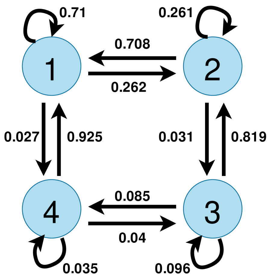
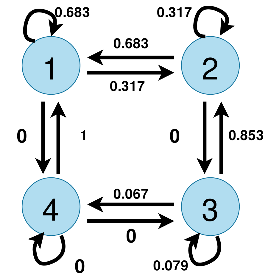
state to state . Hence, this problem becomes one of optimizing transitions
on the graph depicted in Fig. 2, where each state represents a
node on the graph.
Figure 2 depicts the transition matrix for sufficiently large .
While all transition probabilities are
positive for , some of them are for .
For example, and for are given by
Since , it follows from (1) that .
When we regard this problem as a logistics planning as explained in Section I,
means that we do not need to arrange transportation from node to , while retaining a suitable diversity of routes.
Similarly, in optimizing
evacuation routes for residents, it is necessary to disperse people to prevent
overcrowding, while also ensuring that people evacuate in groups to some
extent for safety, requiring a balanced route. Solutions obtained from the -KL control problem are considered to be useful for such problems.
(a)
(b)
Figure 2: Optimal transition probabilities
V -Linear Quadratic Regulator
V-ARicatti equations
The Linear Quadratic Regulator (LQR) is an optimal control problem for linear
systems with quadratic cost functions, which can be solved analytically. In
this section, we formulate an optimal control problem that incorporates Tsallis
entropy as a regularization term for LQR and discuss its properties; See [18, Proposition 1] and [19, Proposition 1] for the Shannon entropy case.
We consider the state and
control input to follow the linear system given by
(35)
The stage cost at each time is given by the following quadratic form:
(36)
In this setting, the optimal control policy is given by the following theorem.
Theorem 3
For Problem 1 with quadratic cost functions (36), the value function is represented as , and the optimal control policy is -Gaussian with mean and variance as follows:
(37)
(38)
(39)
wtih
(40)
(41)
(42)
(43)
(44)
Proof:
From Theorem 1, we have
. Assuming that , the Bellman equation becomes below:
(45)
(46)
(47)
By Lemma 2 in the Appendix, the minimizer of (LABEL:eq:lqr-min) is the density
function of a -Gaussian with mean in (37) and variance in (38).
Since the minimum value does not depend on , it holds that
. Thus, the obtained result is proven inductively.
∎
This theorem shows that the linear feedback with the same gain matrix as LQR with additive noise is optimal.
The resulting closed-loop dynamics is
(48)
Since the -Gaussian has bounded support, the support for the state will also be bounded at any time if the initial state distribution is bounded.
Furthermore, the region of the support can be easily estimated by (12) and (48).
This can be particularly important in real-world applications such as robotics,
where the system can fail if inputs or states move outside their stable operating region.
V-BNumerical example
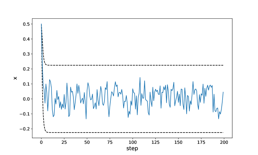
In this section, we solve Problem 1 for , and sufficiently large , the LQR problem () with
(49)
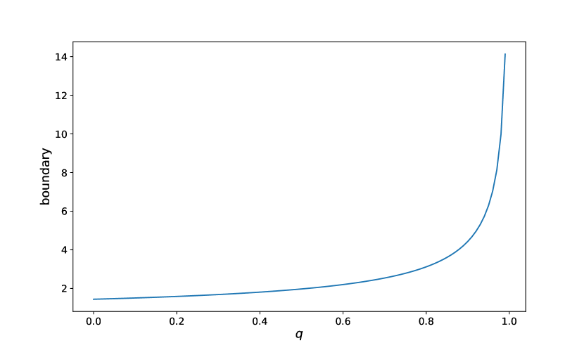
Figure 3 shows an optimally controlled trajectory and its guaranteed region of the support.
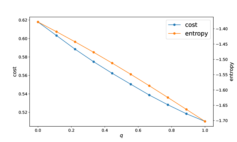
Figure 3: Optimal state trajectories for -LQR, Figure 4: Boundary of support for the additive noise Figure 5: The dependence of control cost and entropy on
Figure 4 shows how the boundary of the additive noise’s support changes with the variation of , i.e., ,
indicating that the larger the , the larger the the support becomes.
Figure 5
illustrate the dependence of control cost and entropy on , respectively, where increasing leads to a decrease in both control cost and entropy.
VI Discussion: Optimal transport problem
In this section, we briefly discuss the optimal transport problem; See [3] for MDP and [18, 19] for the LQR and references therein. The MDP case is formulated as follows:
Problem 3
Consider a Markov process
with transition matrix . For the initial distribution
, terminal distribution , transition cost , transition matrix ,
terminal time , and , find the transition
matrices that minimize the cost function
given by
(50)
under the constraints .
This is an optimal transport over networks where the stage cost is assigned not for the state but for transition.
It should be emphasized that in comparison to Problem 2, a hard constraint is imposed for the final terminal distribution.
When the regularization term is the Shannon entropy,
the Sinkhorn iteration can efficiently solve this problem.
However, in the case of the -KL divergence,
the Sinkhorn iteration solution cannot be directly applied.
This is because the proof and derivation of the Sinkhorn algorithm make extensive use of additivity of the Shannon entropy ,
which does not hold for the Tsallis entropy.
Due to the same reason, the equivalence to the Schrödinger Bridge Problem [18] is not straightforward.
VII Conclusion
We formulated the Tsallis entropy regularized optimal control problem in this study and derived the Bellman equation.
We also investigated optimal control policies for
linearly solvable Markov decision processes and linear quadratic regulators.
Through numerical experiments, we demonstrated the utility of this approach for obtaining solutions
that are both high in entropy and sparse.
Covariance steering and optimal transport problems are currently under investigation.
References
[1]
T. Haarnoja, A. Zhou, P. Abbeel, and S. Levine, “Soft actor-critic: Off-policy maximum entropy deep reinforcement learning with a stochastic actor,” in International Conference on Machine Learning. PMLR, 2018, pp. 1861–1870.
[2]
B. Eysenbach and S. Levine, “Maximum entropy RL (provably) solves some robust RL problems,” in Proceedings. International Symposium on Information Theory, 2005. ISIT 2005., Oct. 2021.
[3]
K. Oishi, Y. Hashizume, T. Jimbo, H. Kaji, and K. Kashima, “Imitation-regularized optimal transport on networks: Provable robustness and application to logistics planning,” Feb. 2024, arXiv:2402.17967 [cs.LG].
[4]
H. Bao and S. Sakaue, “Sparse regularized optimal transport with deformed q,” Entropy, vol. 24, no. 11, p. 1634, Nov. 2022.
[5]
C. Tsallis, “Possible generalization of Boltzmann-Gibbs statistics,” Journal of Statistical Physics, vol. 52, no. 1, pp. 479–487, Jul. 1988.
[6]
K. Lee, S. Choi, and S. Oh, “Sparse markov decision processes with causal sparse Tsallis entropy regularization for reinforcement learning,” IEEE Robotics and Automation Letters, vol. 3, no. 3, pp. 1466–1473, 2018, publisher: IEEE.
[7]
J. Choy, K. Lee, and S. Oh, “Sparse Actor-Critic: Sparse Tsallis entropy regularized reinforcement learning in a continuous action space,” in 2020 17th International Conference on Ubiquitous Robots (UR), Jun. 2020, pp. 68–73, iSSN: 2325-033X.
[8]
M. Gell-Mann and C. Tsallis, Eds., Nonextensive Entropy: Interdisciplinary Applications, ser. Santa Fe Institute Studies on the Sciences of Complexity. Oxford, New York: Oxford University Press, Apr. 2004.
[9]
S. Abe, Y. Okamoto, R. Beig, J. Ehlers, U. Frisch, K. Hepp, W. Hillebrandt, D. Imboden, R. L. Jaffe, R. Kippenhahn, R. Lipowsky, H. V. Löhneysen, I. Ojima, H. A. Weidenmüller, J. Wess, and J. Zittartz, Eds., Nonextensive Statistical Mechanics and Its Applications, ser. Lecture Notes in Physics. Berlin, Heidelberg: Springer, 2001, vol. 560.
[10]
E. P. Borges, “A possible deformed algebra and calculus inspired in nonextensive thermostatistics,” Physica A: Statistical Mechanics and its Applications, vol. 340, no. 1-3, pp. 95–101, Sep. 2004.
[11]
H. Suyari, M. Tsukada, and Y. Uesaka, “Mathematical structures derived from the q-product uniquely determined by Tsallis entropy,” in Proceedings. International Symposium on Information Theory, 2005. ISIT 2005. Adelaide, Australia: IEEE, 2005, pp. 2364–2368.
[12]
S. Furuichi, K. Yanagi, and K. Kuriyama, “Fundamental properties of Tsallis relative entropy,” Journal of Mathematical Physics, vol. 45, no. 12, pp. 4868–4877, Dec. 2004.
[13]
C. Vignat and A. Plastino, “Central limit theorem, deformed exponentials and superstatistics,” Jun. 2007, arXiv:0706.0151 [cond-mat].
[14]
S. Furuichi, “On the maximum entropy principle and the minimization of the Fisher information in Tsallis statistics,” Journal of Mathematical Physics, vol. 50, no. 1, p. 013303, Jan. 2009.
[15]
G. Neu, A. Jonsson, and V. Gómez, “A unified view of entropy-regularized Markov decision processes,” May 2017, arXiv:1705.07798 [cs, stat].
[16]
B. Peters, V. Niculae, and A. F. T. Martins, “Sparse sequence-to-sequence models,” Jun. 2019, arXiv:1905.05702 [cs].
[17]
K. Ito and K. Kashima, “Kullback–Leibler control for discrete-time nonlinear systems on continuous spaces,” SICE Journal of Control, Measurement, and System Integration, vol. 15, no. 2, pp. 119–129, Jun. 2022.
[18]
——, “Maximum entropy optimal density control of discrete-time linear systems and Schrödinger bridges,” IEEE Transactions on Automatic Control, vol. 69, no. 3, pp. 1536–1551, 2024.
[19]
——, “Maximum entropy density control of discrete-time linear systems with quadratic cost,” Sep. 2023, arXiv:2309.10662 [math.OC].
Appendix A Tsallis entropy regularized optimization
We prove two lemmas on optimization problems with a Tsallis entropy regularization term.
Lemma 1
For a real-valued function and ,
(51)
where is a constant determined by
is a unique minimizer of
(52)
Proof:
From the KKT conditions, for any optimal solution there exists such that