Spectrum AUC Difference (SAUCD): Human-aligned 3D Shape Evaluation

Abstract

Existing 3D mesh shape evaluation metrics mainly focus on the overall shape but are usually less sensitive to local details. This makes them inconsistent with human evaluation, as human perception cares about both overall and detailed shape. In this paper, we propose an analytic metric named Spectrum Area Under the Curve Difference (SAUCD) that demonstrates better consistency with human evaluation. To compare the difference between two shapes, we first transform the 3D mesh to the spectrum domain using the discrete Laplace-Beltrami operator and Fourier transform. Then, we calculate the Area Under the Curve (AUC) difference between the two spectrums, so that each frequency band that captures either the overall or detailed shape is equitably considered. Taking human sensitivity across frequency bands into account, we further extend our metric by learning suitable weights for each frequency band which better aligns with human perception. To measure the performance of SAUCD, we build a 3D mesh evaluation dataset called Shape Grading, along with manual annotations from more than 800 subjects. By measuring the correlation between our metric and human evaluation, we demonstrate that SAUCD is well aligned with human evaluation, and outperforms previous 3D mesh metrics.

1 Introduction

With the recent progress of 3D reconstruction and processing techniques, 3D mesh shapes have increasing applications in fields such as video games, industrial design, 3D printing, etc. In these applications, assessing the visual quality of the 3D mesh shape is a crucial task. To meet the requirements of various applications, a promising evaluation metric should not only reflect the geometry measurement but also align with human visual perception. Considering that human beings perceive 3D meshes in both overall shape and local details, it is a challenging task to find an evaluation metric that can align well with humans.

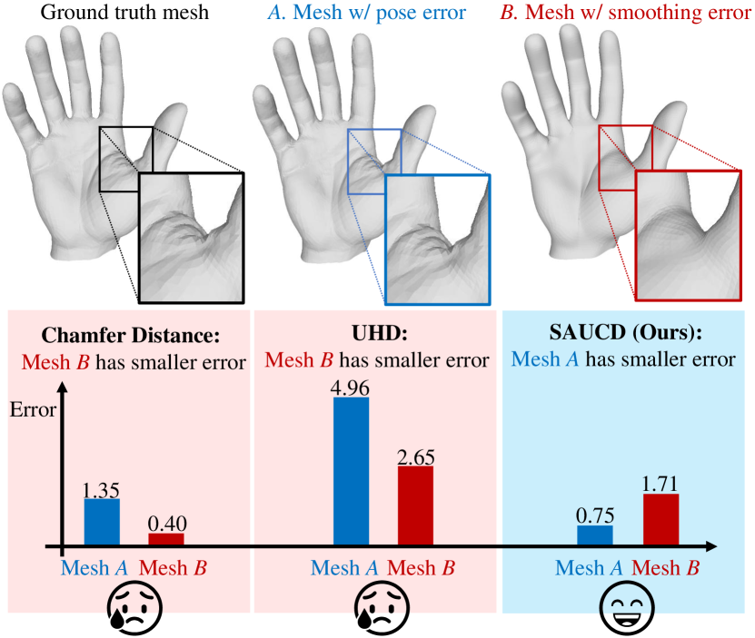
Figure 1: An example of how previous spatial domain 3D shape metrics (Chamfer Distance [7] and UHD [69]) deviate from human evaluation. we create Mesh $A$ by adding a small pose error to the ground truth mesh, and by applying a large smoothing kernel to ground truth, we create Mesh $B$. Contrary to human perception, previous spatial domain metrics evaluate Mesh $B$ better than Mesh $A$. This indicates that while they are sensitive to general shape differences, they tend to overlook high-frequency details. Note that different metrics use different units of measurement.

Previous metrics have the following disadvantages in this scenario. Traditional spatial domain measurements such as Chamfer Distance [7] which calculates the mean distance between a vertex on one mesh and its nearest vertex on the other mesh, can accurately measure the spatial distance. However, it does not guarantee capturing all shape details. In fact, such measurements in the spatial domain often overlook finer shape details, as the details tend to get overwhelmed by the overall shape. Fig. 1 illustrates the discrepancy between spatial measurements and human evaluation as mesh details change. Specifically, When we remove the wrinkles from the ground truth mesh (resulting in Mesh B), the errors detected by previous metrics are not as significant as when we slightly change the pose of the hand (Mesh A). However, humans tend to sense a significant difference between ground truth and Mesh B, but barely recognize the difference between ground truth and Mesh A. To mitigate this problem, previous works propose learning-based approaches, such as Single Shape Fréchet Inception Distance (SSFID) [68] based on learnable features from 3D shape. They compare the difference between the test mesh and the ground truth mesh in the latent feature space, and the design is expected to better align human perception. However, such learning-based methods would require a large amount of data to train the network. Their accuracy and generalizability are limited by the size of the dataset, data distribution, and annotation quality, not to mention the potential bias in collecting human perception feedback, which could mislead the learned metrics. An analytic metric that can better explain the shape difference is thus preferred.

To address the above limitations, we design an analytic-based 3D shape evaluation metric named Spectrum Area Under the Curve Difference (SAUCD). Our metric measures mesh shape differences with a balanced consideration of both overall and detailed shape, making it better aligned with human evaluation. To allow our metric to capture detail variations, we leverage the 3D shape spectrum to decompose different levels of shape details from the overall shape, with details corresponding to higher-frequency components. The advantage of transforming the shape signal into the spectrum domain is that the high-frequency details are explicitly separated from the low-frequency overall shape. Therefore, it provides appropriate consideration to the information in different frequency bands, not just the low-frequency information of the overall shape in the dominant place. Thus, the details that human perception cares about will be better represented. Besides, the frequency analysis method allows the metric to be mostly analytic and better explained.

We design SAUCD following the above inspiration. To begin with, both the test mesh and the ground truth mesh are transformed from the spatial to the spectrum domain using the discrete Laplace-Beltrami operator (DLBO), which encodes the mesh geometry information into a semidefinite Laplacian matrix. Once in the spectrum domain, we compare the regions under the two spectrums. Our Spectrum Area Under the Curve Difference metric is defined as the area of the non-overlapping region under the two spectrums – a larger area indicates a greater difference. Moreover, to better align with human evaluation, we further extend our design by learning a spectrum weight for SAUCD. However, different from previous learning-based approaches that use deep networks, large datasets, and extensive learning processes, our learning-based method requires the training of a weight vector. This vector measures the sensitivity of human perception across frequency bands, making the learned metric better aligned with human perception. We then evaluated the effectiveness of SAUCD on our provided user study benchmark dataset named Shape Grading. Using Shape Grading, we compare our metrics with previous metrics by calculating the correlation between each metric and human scoring. In summary, our contributions are listed as follows.

• We design an analytic-based 3D mesh shape metric named Spectrum AUC Difference (SAUCD), which evaluates the difference between a 3D mesh and its ground truth mesh. Our metric considers both the overall shape and intricate details, to align more closely with human perception.

• We further extend our design to a learnable metric. The extended metric explores the human perception sensitivity in different frequency bands, which further improves this metric.

• We build a user study benchmark dataset named Shape Grading which is annotated by more than 800 subjects. The provided dataset verifies that both versions of our metrics are consistent with human evaluation and outperform previous methods. This dataset can also facilitate 3D mesh metric evaluation in future research.

Our experiments show that both SAUCD and its extended version outperform previous methods with good generalizability to different types of objects.

2 Related Works

Metrics in 3D mesh reconstruction. Chamfer Distance [7] is a popular metric used in 3D mesh reconstruction tasks such as those in [36, 66, 81, 73, 54, 50, 78, 33]. Other spatial domain metrics, such as 3D Intersection over Union (IoU) in [27, 13, 42, 25, 59, 52]. F-score in [64, 22, 4, 60], and Unidirectional Hausdorff distance (UHD) in [69] are commonly focused on the geometry accuracy of mesh shapes. These metrics can provide accurate geometry measurements, but they are not designed to align with human evaluation. Deep-learning-based methods such as Single Shape Fréchet Inception Distance [68] are also used in 3D reconstruction. While these metrics have the capacity to adapt from human evaluation, they are more like black boxes, with performances subject to dataset size and annotation bias. Moreover, most previous works miss out on user study validation to verify if their metrics align with human evaluation.

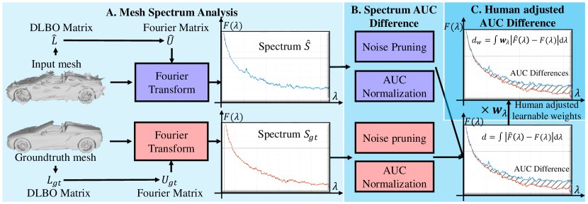
Figure 2: Our SAUCD metric is designed as follows: A. We use mesh Fourier Transform to analyze the spectrums of test and ground truth mesh. B. We compare the difference between two spectrum curves by calculating the Area Under the Curve (AUC) difference. C. We further extend our metric by multiplying the AUC difference with a learnable weight to capture human sensitivity in each frequency band.

3D shape generation metrics. Multiple metrics have been used in 3D shape generation, such as Minimal Matching Distance (MMD) [3], Jensen-Shannon Divergence (JSD) [34], Total Mutual Difference (TMD) [69], Fréchet Pointcloud Distance (FPD) [55], etc.. These metrics are designed to measure the differences between the generated distributions, while our task is to build a metric to compare the shape of two meshes.

3D mesh compression and watermarking metrics. Previous works [62, 10, 35, 16] focused on evaluating mesh errors in mesh compression and watermarking. Since compression and watermarking pursue mesh errors that cannot be detected by humans, they mainly focus on barely noticed errors. However, our task is to build a metric that can handle generally occurring errors that happen in 3D reconstruction tasks and applications.

3 Proposed Method

Our task is to design a metric aligned with human evaluation to measure the shape difference between a test triangle mesh and its corresponding ground truth triangle mesh. Specifically, given a test mesh $\hat{M}$ and its ground truth mesh $M_{gt}$, Spectrum AUC Difference (SAUCD) can be abstracted as

$$d=D(\hat{M},M_{gt}).$$ (1)

$d$ is the distance between the test and the ground truth mesh. In this section, we will elaborate on how the distance function $D(\cdot)$ is designed.

3.1 Overview

As shown in Fig. 2, our metric is calculated via the following steps: First, we use mesh Fourier transform to analyze the spectrums of the test and ground truth mesh (in Sec. 3.2). Then we leverage each frequency band by calculating the Area Under the Curve (AUC) difference of the spectrum curves (in Sec. 3.3). Moreover, we further extended our metric by multiplying the AUC difference with a learnable weight to capture the human sensitivity on each frequency band (in Sec. A.2). We will discuss each step in detail.

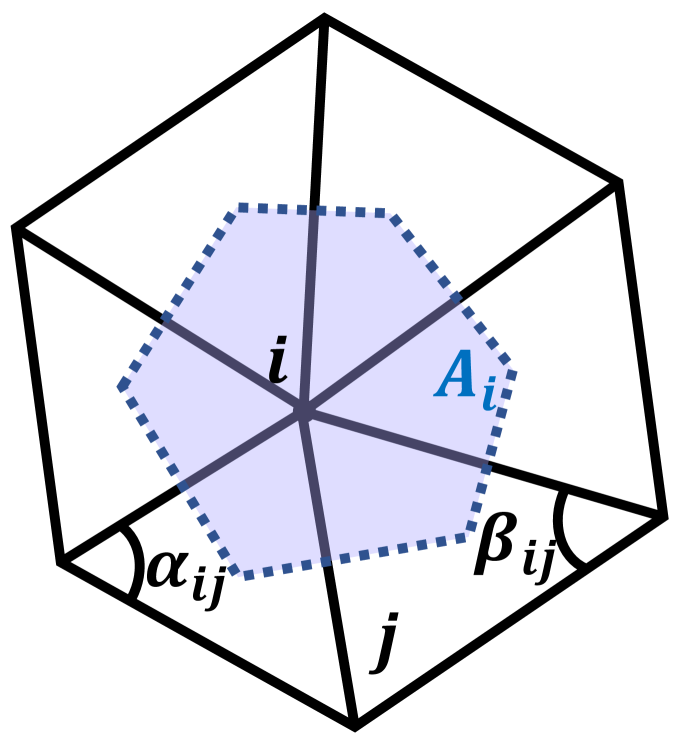
Figure 3: Variables defined in our discrete Laplace-Beltrami operator design.

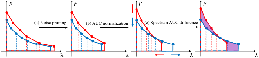
Figure 4: Spectrum Area Under the Curve Difference. We design our metric using the AUC difference of the spectrums. The blue curve and red curve are the test and ground truth mesh spectrum, respectively. The purple area in the last graph is the Spectrum AUC Difference. Please find details in Sec. 3.3.

3.2 Mesh spectrum analysis

In order to capture the overall shape as well as shape details, we choose to decompose the mesh signal into a spectrum. Considering the mesh as a function on a discretized manifold space, we can calculate the spectrum using the manifold space Fourier transform. In Hilbert space, the Fourier operator is defined as the eigenfunctions of the Laplacian operator [18]. The same definition and similar theories are extended to continuous and discrete manifold space by [11, 6]. The Laplacian operator on discrete manifold spaces, i.e. mesh space in our task, is named the Discrete Laplace-Beltrami operator (DLBO). Similar to the Laplacian operator in image space that encodes the pixel information by capturing the local pixel differences [48, 53, 65, 57, 32, 45], DLBO encodes the mesh shape information by capturing the local shape fluctuation. The “Cotan formula” defined in [40] is the most widely used discretization, which can be represented in matrix form as

$$\small L_{ij}=\left\{\begin{array}[]{cc}\sum_{j\in N(i)}\frac{1}{2A_{i}}(\cot\alpha_{ij}+\cot\beta_{ij}),&i=j\\ -\frac{1}{2A_{i}}(\cot\alpha_{ij}+\cot\beta_{ij}),&i\neq j\land j\in N(i)\\ 0,&i\neq j\land j\notin N(i),\end{array}\right.$$ (2)

where $L\in\mathbb{R}^{N\times N}$ is the DLBO matrix, with $N$ the vertex number of the mesh. $L_{ij}$ indicates its entry in $i$th row and $j$th column, which represents the edge weight between vertex $v_{i}$ and $v_{j}$. $A_{i}$ is the mixed Voronoi area of vertex $v_{i}$ on the mesh. As shown in Fig. 4, the $v_{i}$’s mixed Voronoi area is defined as the area of the polygon in which the vertices are the circumcenters of $v_{i}$’s surrounding faces. $N(i)$ is the index set of $v_{i}$’s adjacent vertices. If $v_{i}$ and $v_{j}$ are adjacent, $\alpha_{ij}$ and $\beta_{ij}$ are the opposite angles of edge $(v_{i},v_{j})$ in each of the edge’s two neighbor triangle faces, respectively (shown in Fig. 4). If not, $\alpha_{ij}$ and $\beta_{ij}$ are not defined and $L_{ij}$ is 0. As shown in Fig. 2, the DLBO matrix is used for mesh Fourier transform to get mesh spectrum. We calculate the Fourier operator $U^{\top}$, which is the eigenfunction of $L$ as

$$L=U\Lambda U^{\top},$$ (3)

where $\Lambda$ is a diagonal matrix whose diagonal elements are Fourier mesh frequencies.

To ensure the mesh frequencies are non-negative, we need the DLBO matrix $L$ to be positive semidefinite. Our experiment in Fig. 7 gives an example of the counterintuitive results when there are negative frequencies. However, the Cotan formula in Eq. 2 does not guarantee to be positive semidefinite. We provide a simple example in Appendix 3 in which $L$ is not positive semidefinite when the mesh is not Delaunay triangulated and the mixed Voronoi areas are not all equal to each other. In our metric design, we made two small changes to the original Cotan formula to make it positive semidefinite. a) Inspired by the symmetric normalization of the topology Laplacian matrix in [14], we make $L$ symmetric by changing the normalization parameter $A_{i}$ into a symmetric normalized manner $A_{i}^{\frac{1}{2}}A_{j}^{\frac{1}{2}}$. b) We replace $\cot\alpha_{ij}+\cot\beta_{ij}$ with $|\cot\alpha_{ij}+\cot\beta_{ij}|$. This ensures all the edge weights in the Laplacian matrix to be non-negative. Thus, our revision of DLBO is defined as

$$\footnotesize L_{ij}=\left\{\begin{array}[]{cc}\frac{1}{2}\sum_{j\in N(i)}A_{i}^{-\frac{1}{2}}A_{j}^{-\frac{1}{2}}|\cot\alpha_{ij}+\cot\beta_{ij}|,&i=j\\ -\frac{1}{2}A_{i}^{-\frac{1}{2}}A_{j}^{-\frac{1}{2}}|\cot\alpha_{ij}+\cot\beta_{ij}|,&i\neq j\land j\in N(i)\\ 0,&i\neq j\land j\notin N(i).\end{array}\right.$$ (4)

We prove that our revision of the Cotan formula is positive semidefinite in Appendix B. In Tab. 5, our experiments show that our DLBO matrix design outperforms the origin Cotan formula in [40], and the topology Laplacian matrix defined in [14].

Finally, we obtain the mesh spectrum by acting Fourier operator on the mesh vertices

$$F_{i}=\sqrt{G_{i,x}^{2}+G_{i,y}^{2}+G_{i,z}^{2}},G=U^{\top}v,$$ (5)

where $v\in\mathbb{R}^{N\times 3}$ indicates the 3D coordinates of $N$ mesh vertices. The result spectrum $F\in\mathbb{R}^{N}$. Fig. 5 shows an example of the mesh spectrum (left side) and how the meshes look in different frequency bands (right side). This provides an illustration of the information contained in different frequency bands of the mesh spectrum.

3.3 Spectrum AUC Difference

To reduce the noise and normalize the mesh scale, we also design noise pruning and AUC normalization procedures before calculating the Spectrum AUC Difference.

Noise pruning. As shown in Fig. 4 process (a), we prune a small portion of the highest frequency information to reduce the interference of noise. From the observation of the first two meshes (A and B) in Fig. 5, we can see that humans can barely notice the shape differences when the highest frequency parts are removed. Thus, if we try to evaluate the mesh shape that aligns with human perception, it is reasonable to remove high-frequency noise without losing much information that humans care about. Empirically, we choose to prune the highest $0.1\%$ frequency information as noise. Our experiments in Tab. 5 show that this portion is more consistent with human perception while preserving good mesh quality.

AUC normalization. Given a spectrum $F(\lambda)$, its Area Under the Curve (AUC) can be defined as $\int_{\infty}F(\lambda)d\lambda$. AUC normalization means using spectrum AUC to normalize the mesh scale. If the mesh scale increases by $s$ times in length, the mixed Voronoi area, i.e. $A_{i}$ in Eq. 4, will decrease by $s^{2}$ times. Thus, each element in the DLBO matrix $L$ will also decrease by $s^{2}$ times. Then, according to Eq. 3, the frequency $\lambda$ will decrease $s^{2}$ times to $\lambda/s^{2}$, and according to Eq. 5, the spectrum amplitude $F$ will change to $sF$ because $v$ is increased by $s$ time and $U^{\top}$ is still orthonormal. Then the area under the spectrum curve (the area boxed with red or blue lines in Fig. 4) changes as $A^{\prime}=\int sF(\lambda)d\lambda/s^{2}=\frac{1}{s}A$.

In our approach, we normalize the area under the spectrum curve $A$ to 1 to resolve the scale difference, which means $s=A$, $\lambda$ decreases by $A^{2}$ times, and spectrum amplitude $F$ increases by $A$ times (Fig. 4 process (b)). AUC normalization fairly normalizes the scale of objects in different shapes by only changing the scale, not shape details. It normalizes the spectrum AUC of all mesh to 1, making the mesh spectrums differ only in distributions. Our experiments in Tab. 5 demonstrate this design can bring a fairer comparison of the spectrums and improve the human consistency of the metric. The experiment also demonstrates that this design outperforms the spatial domain scale normalization.

Spectrum AUC Difference. In order to capture the difference between two mesh shapes in the spectrum domain, we design Spectrum AUC Difference (SAUCD) on the spectrum analysis results after noise pruning and AUC normalization:

$$d=D(\hat{M},M_{gt})=\int_{\lambda}|\hat{F}(\lambda)-F_{gt}(\lambda)|d\lambda,$$ (6)

where $\hat{F}$ and $F_{gt}$ are the test and groundtruth mesh spectrum. As shown in Fig. 4 process (c), our metric is defined as the AUC difference of the two spectrum curves (the purple area). In Tab. 5, we compare our design with an alternative design which changes the amplitude difference $|\hat{F}(\lambda)-F_{gt}(\lambda)|$ to energy difference $|\hat{F}(\lambda)^{2}-F_{gt}(\lambda)^{2}|$. The result shows our design is more consistent with human evaluation. Besides, experiments in Tab. 2 show our SAUCD metric aligns well with human evaluation, and outperforms SOTA metrics under multiple evaluation methods. Experiments in Fig. 8 show SAUCD has the capability to improve mesh detail qualities in 3D reconstruction when adapted into training loss.

3.4 Human-adjusted Spectrum AUC Difference

We also provide an extended metric version, in which we design a learnable weight parameter along the frequency bands. The weight parameter indicates the adjustment of human sensitivity to each frequency band. Specifically, we design the extended metric as

$$d_{w}=D_{w}(\hat{M},M_{gt})=\int_{\lambda}w(\lambda)|\hat{F}(\lambda)-F_{gt}(\lambda)|d\lambda.$$ (7)

$w(\lambda)$ is weight parameters indicating human sensitivity along frequency bands. Our training loss is defined as

$$\mathcal{L}=\lambda_{p}\mathcal{L}_{plcc}+\lambda_{sr}\mathcal{L}_{srocc}+\lambda_{r}\mathcal{L}_{regu},$$ (8)

where $\mathcal{L}_{plcc}$ and $\mathcal{L}_{srocc}$ are Pearson correlation loss and Spearman rank order loss. They are defined the same as Pearson’s linear correlation [47] and Spearman’s rank order correlation [56]. $\mathcal{L}_{regu}=1/N\sum_{i}(w_{i}-1)^{2}$ is the regularization loss, which regularizes weight $w_{i}$ close to 1. $\lambda_{p}$, $\lambda_{sr}$, and $\lambda_{r}$ are the loss weights of $\mathcal{L}_{plcc}$, $\mathcal{L}_{srocc}$, and $\mathcal{L}_{regu}$. More details of the loss functions can be found in Appendix A. Our experiments in Sec. 4.3 show that after adjustment, the consistency between our metric output and human-annotated ground truth is improved.

dataset	Raw	w/ IQR removal
number of valid scores	24304	23775
Scoring range	$[0,6]$	$[0,6]$
$95\%$ confidence interval	0.318	0.303
Relative $95\%$ confidence interval	$5.33\%$	5.04%

Table 1: Dataset statistics and error analysis.

	1	2	3	4	5	6	7	8	9	10	11	12	Overall
Chamfer Distance [7]	0.54	0.15	-0.10	0.57	-0.06	-0.12	-0.20	0.07	0.04	0.30	-0.20	0.17	0.097
Point-to-Surface	0.45	0.19	-0.04	0.66	-0.08	-0.25	-0.32	-0.20	0.01	0.13	-0.21	-0.12	0.017
Normal Difference	0.46	0.11	0.06	0.28	0.11	0.21	0.29	0.47	0.27	0.39	0.11	0.27	0.253
IoU [25]	0.60	0.63	0.01	0.51	0.30	0.02	-0.07	0.20	0.14	0.47	-0.09	-0.01	0.225
F-score [64]	0.58	0.09	0.05	0.33	0.03	0.06	0.16	0.34	0.27	0.25	0.01	0.34	0.208
SSFID [68]	0.71	0.74	-0.04	0.74	0.39	0.24	0.13	0.32	0.25	0.64	0.25	-0.02	0.363
UHD [69]	0.29	0.22	0.11	0.15	-0.04	0.18	0.41	0.55	0.13	0.18	0.25	0.33	0.231
SAUCD (Ours)	0.73	0.21	0.60	0.63	0.31	0.51	0.83	0.65	0.77	0.80	0.69	0.08	0.567
Adjusted SAUCD (Ours)	0.79	0.19	0.56	0.64	0.36	0.54	0.79	0.76	0.75	0.77	0.67	0.36	0.598

(a)

a. Pearson’s linear correlation coefficient.

	1	2	3	4	5	6	7	8	9	10	11	12	Overall
Chamfer Distance [7]	0.33	0.14	-0.09	0.43	-0.08	-0.06	-0.15	0.17	-0.04	0.24	-0.16	0.22	0.079
Point-to-Surface	0.42	0.39	0.14	0.59	0.11	0.05	-0.10	0.20	0.18	0.40	-0.11	0.18	0.205
Normal Difference	0.44	0.22	0.33	0.42	0.19	0.29	0.33	0.56	0.33	0.32	0.21	0.34	0.331
IoU [25]	0.57	0.61	0.28	0.50	0.36	0.21	0.12	0.31	0.262	0.56	0.03	0.30	0.342
F-score [64]	0.47	0.25	0.20	0.52	0.21	0.11	0.07	0.36	0.30	0.42	-0.01	0.35	0.27
SSFID [68]	0.63	0.81	0.28	0.70	0.33	0.23	0.10	0.33	0.32	0.65	0.16	0.34	0.407
UHD [69]	0.38	0.20	0.11	0.32	0.13	0.35	0.41	0.60	0.06	0.27	0.37	0.35	0.296
SAUCD (Ours)	0.79	0.25	0.57	0.59	0.36	0.56	0.83	0.79	0.69	0.69	0.83	0.24	0.598
Adjusted SAUCD (Ours)	0.83	0.21	0.55	0.59	0.38	0.60	0.82	0.80	0.69	0.68	0.75	0.42	0.611

(b)

b. Spearman’s rank order correlation coefficient.

	1	2	3	4	5	6	7	8	9	10	11	12	Overall
Chamfer Distance [7]	0.25	0.14	-0.08	0.31	-0.04	-0.02	-0.09	0.15	0.013	0.19	-0.07	0.22	0.080
Point-to-Surface	0.33	0.30	0.07	0.45	0.10	0.08	-0.03	0.17	0.13	0.30	-0.01	0.16	0.171
Normal Difference	0.34	0.16	0.17	0.31	0.18	0.22	0.26	0.44	0.25	0.23	0.16	0.27	0.250
IoU [25]	0.42	0.44	0.24	0.37	0.28	0.22	0.14	0.26	0.20	0.41	0.10	0.23	0.275
F-score [64]	0.37	0.17	0.14	0.42	0.15	0.11	0.09	0.28	0.23	0.34	0.01	0.30	0.216
SSFID [68]	0.48	0.62	0.24	0.51	0.25	0.24	0.12	0.29	0.26	0.48	0.17	0.23	0.322
UHD [69]	0.27	0.13	0.07	0.22	0.09	0.26	0.29	0.42	0.048	0.19	0.28	0.24	0.209
SAUCD (Ours)	0.60	0.16	0.42	0.41	0.27	0.45	0.65	0.57	0.55	0.47	0.60	0.19	0.445
Adjusted SAUCD (Ours)	0.64	0.14	0.40	0.41	0.29	0.48	0.63	0.59	0.55	0.45	0.57	0.29	0.453

(c)

c. Kendall’s rank order correlation coefficient.

Table 2: Correlations between different metrics and human annotation. “SAUCD” is our basic version metric. “Adjusted SAUCD” is the human-adjusted version of our metric. The ranges of all three correlation coefficients are $[-1,1]$, and the higher the better.

4 Experiments

4.1 Dataset

We build a user study benchmark dataset Shape Grading to evaluate whether our metric is aligned with human evaluation. The dataset contains the human evaluation scores for a variety of distorted meshes. Using this dataset, we can calculate the correlation between metric outputs and human evaluation scores to see how aligned the test metrics are to human evaluation.

Dataset design. We choose 12 objects as ground truth 3D triangle mesh from public object/scene/human mesh datasets such as [41, 28, 63] and commercial datasets such as [1, 2]. These objects are picked from different categories including humans, animals, buildings, plants, etc.. For each object, we synthesize 7 different types of distortions which commonly occur in 3D reconstruction. For each distortion type we synthesize 4 distortion levels, which gives us $7\times 4=28$ distorted objects for every ground truth object. We rotate and render each distorted object into 3 videos using different materials for the mesh. In total, we generate $12\times 28\times 3=1,008$ distorted mesh videos. Appendix D shows the meshes and distortion types we use in our dataset along with rendered video examples.

Human scoring procedure. We use a pairwise comparison scoring process similar to [49]. Each subject will evaluate all 28 distorted objects of one ground truth object with a certain material. The scoring follows a Swiss system tournament principle used in [49], in which each subject takes 6 rounds of pairwise comparison to score the distorted meshes. After 6 rounds of scoring, the meshes are scored from 0 to 6. 0 means the object loses in every round and 6 means it wins in every round. This process will largely reduce the biases among subjects, since the subjects are compelled to distribute an equal amount of points to the 28 distorted objects. The process will take about 15 minutes for each subject, avoiding the fatigue problem in [9]. For every object rendered with every material, we have 24 to 25 subjects scoring it. In total, we have 868 subjects (536 males, 316 females, and 16 others) who give us $868\times 28=24304$ scores. More details of the scoring procedure can be found in Appendix E.

Outlier detection. We use the interquartile range (IQR) method [17] which is widely used in statistics to detect and remove outliers. For each distorted mesh, we first find the 25 percentile and the 75 percentile of the scores. The score range in between is called the IQR range. We remove the scores that are 1.5IQR smaller than the 25 percentile or 1.5IQR larger than the 75 percentile. Our dataset error analysis in Tab. 1 shows, that by removing $2.2\%$ of the scores using IQR, we can decrease the uncertainty of the final scoring result by nearly $6\%$.

Dataset error analysis. We analysis the average $95\%$ confidence interval of our dataset scores in Tab. 1. The confidence interval of score $x$ can be calculated as ${\sigma}_{\bar{x}}=z_{0.95}\times\sigma/\sqrt{N}$ where $\sigma$ is the standard derivation of $x$, $N$ is the number of valid scores, and $z_{0.95}\approx 1.96$. We report the average $95\%$ confidence interval and the relative $95\%$ confidence interval (which is the confidence interval divided by the scoring range). The result shows that dataset scoring is accurate with a $5\%$ error range with IQR outlier removal.

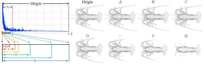
Figure 5: An example of mesh spectrum curve: We do mesh Fourier transform on the “Origin” mesh and show the spectrum in the left graph. The $\lambda$-axis is the eigenvalues of the DLBO matrix, the larger the higher frequency. We also show how mesh changes when gradually removing high-frequency information (mesh A to G). The frequency bands of the meshes are shown as the colored arrows in the left graph.

Evaluation methods. We use 3 different evaluation methods to evaluate the correlation between our metrics and the human scoring (ground truth) on our Shape Grading benchmark dataset. Pearson’s linear correlation coefficient (PLCC) [47] is used to evaluate the linear alignment between our metric and human perception. We also used Spearman’s rank order correlation coefficient (SROCC) [56] and Kendall’s rank order correlation coefficient (KROCC) [30] to evaluate the ranking order correlation between our metric and human perception. The possible ranges of 3 metrics are all $[-1,1]$. Higher numbers mean stronger correlations. More details of the three evaluation methods can be found in Appendix A.

4.2 Implementation details

We implement our basic version metric following Eq. 6. $\hat{F}(\lambda)$ and $F_{gt}(\lambda)$ in Eq. 6 are both piece-wise functions, so we implement the integration by simply adding every piece area together. We implement our human-adjusted version following Eq. 7. We use a 20-dimensional weight $w(\lambda)$ to avoid overfitting. We interpolate $w$ to all frequencies of the ground truth and test meshes and element-wisely multiply them to the spectrums. In spectrum weight training, SROCC and PLCC are used as part of the loss function as Eq. 8. KROCC is not used in training but only for testing. We use a k-fold strategy for training the human-adjusted weight. Each time we choose 1 object for testing and the rest 11 objects for training, which means $k=12$. More implementation details can be found in Appendix A.

4.3 Quantitive and qualitative results

SOTA comparison. Tab. 2 shows our results compared to previous 3D mesh shape metrics. We evaluated the correlation between each metric and the human scoring via three different evaluation methods. We observe that a) without any learning-based design, our metric outperforms the SOTA learning-based (SSFID) and non-learning-based metrics (Chamfer Distance, IoU, F-score, and UHD), b) our extended version metric with learned weights has better linearity and slightly better ranking order correction with human evaluation, and c) our results on different objects show that our metrics have good generalizability.

Spectrum example. We first show an example of mesh spectrum in Fig. 5. We decompose the “origin” mesh using the Fourier Transform and get the resulting spectrum (top-left graph). The meshes on the right (from mesh A to G) are generated by gradually removing high-frequency information. The frequency bands of the meshes are shown as colored arrows in and under the graph. As we see, the details gradually disappear as we remove high-frequency information.

Frequency band separation. We explored the consistency between human perception and the information obtained from every frequency band. Specifically, we separate the frequency band exponentially and build metrics only using information from that frequency band. The results are shown in Tab. 5, we find the frequency bands $[0,0.001]$ and $[0.01,0.03]$ have the best consistency with human perception. Moreover, it shows that if we put all frequencies together, they can achieve better results.

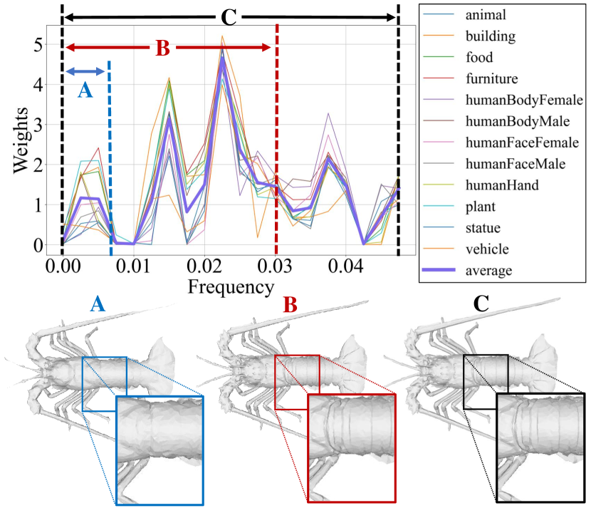
Figure 6: Learned spectrum weights on all 12 folds. The name of colorful thin lines means the test object name of that fold. The bold purple line is the average weights of all folds. We also show some examples of mesh shape information in different frequency bands. Frequency band A is $[0,0.0075)$, B is $[0,0.03)$, and C is $[0,0.05)$.

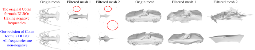
Figure 7: Counterintuitive low-frequencies information if some of the mesh frequencies are negative. We can see if we remove the high-frequency part of the mesh (resulting in “Filtered mesh 1” and “Filtered mesh 2”) using the original Cotan formula, the mesh’s low-frequency parts show artifacts (sharp shapes). The red circles show the artifacts in the left object. The right object shows a case when these artifacts occur much more often. These artifacts do not occur using our revised Cotan formula DLBO.

Frequency band	PLCC $\uparrow$	SROCC $\uparrow$	KROCC $\uparrow$
$[0,0.001)$	0.434	0.515	0.376
$[0.001,0.003)$	0.240	0.409	0.281
$[0.003,0.01)$	0.255	0.455	0.340
$[0.01,0.03)$	0.421	0.528	0.391
$[0.03,0.1)$	0.287	0.351	0.250
$[0.1,\infty)$	0.318	0.192	0.155
$[0,\infty)$	0.567	0.598	0.445

Table 3: Results when building metrics using each frequency band separately. The bottom row is our proposed metric.

Pruning Portion	PLCC $\uparrow$	SROCC $\uparrow$	KROCC $\uparrow$
$0\%$	0.513	0.549	0.393
$0.1\%$	0.567	0.598	0.445
$1\%$	0.554	0.602	0.462
$10\%$	0.517	0.581	0.442
$20\%$	0.503	0.587	0.445

Table 4: Results with different pruning portions. The metric achieves better results with pruning portion to be $0.1\%$ or $1\%$. We use pruning portion as $0.1\%$ in our design.

Modules	PLCC $\uparrow$	SROCC $\uparrow$	KROCC $\uparrow$
Topology Laplacian [14]	0.298	0.327	0.235
Cotan formula [40]	0.417	0.470	0.340
Energy difference	0.268	0.315	0.215
w/o normalization	0.257	0.507	0.353
Spatial normalization	0.269	0.542	0.392
Ours	0.567	0.598	0.445

Table 5: Module replacement. We replace each module of our metric with alternative designs to verify the design of each module.

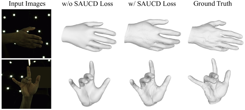
Figure 8: We Adapt SAUCD into a loss function and use it in monocular-image-based 3D hand reconstruction. From left to right: input images, reconstruction result w/o SAUCD loss, reconstruction result w/ SAUCD loss, and ground truth mesh. We can see that the enhancement of SAUCD loss in mesh details is clearly noticeable.

Trained weight. We show our trained weights in Human-adjusted metric in Fig. 6. Different lines represent different folds, and the bold purple line is the average weight. We can see the weights trained on each fold have similar patterns. We also observe that the weight curves have a small peak in the range A and two much larger peaks between A and B, which means our extended metric relies more on the information between A and B. We show an example of mesh shapes in the range A, B, and C at the bottom of Fig. 6. Mesh A obviously has fewer details than Mesh B, and the weight curve shows that this difference is what the learning process tries to emphasize.

Negative frequencies. In Fig. 7 we illustrate how our revised Cotan formula DLBO in Eq. 4 improves frequency analysis compared to the original Cotan formula in Eq. 2 [40]. The first and second rows are the results of the original Cotan formula DLBO and our revised Cotan formula DLBO, respectively. The original Cotan formula can yield negative frequencies due to its lack of positive semidefiniteness, whereas our revision ensures all frequencies are non-negative. For both objects in the figure, we remove different portions of high-frequency information and show the remaining low-frequency parts (resulting in “Filtered mesh 1” and “Filtered mesh 2”). For the left object, notice the counterintuitive sharp shapes in the red circle when using the Cotan formula. The right object is a much more severe case. Sharp shapes in low-frequency parts show improper decomposition and high-frequency aliasing with low-frequency shapes, making the Cotan formula unsuitable for spectral mesh comparison. In contrast, our revised formula yields smooth low-frequency components without these artifacts.

Noise pruning portion. Tab. 5 shows our SAUCD metric performance by changing the noise pruning portion (Sec. 3.3). The metric achieves better results when the pruning portion is $0.1\%$ or $1\%$. In our proposed metric, we choose the pruning portion to be $0.1\%$ to best avoid possible high-frequency information loss.

Module replacement. Tab. 5 shows our SAUCD metric performance by replacing some modules with alternative designs. First, we replace our revision of the discrete Laplace-Beltrami operator in Eq. 4 with topology Laplacian matrix in [14] and “Cotan formula” in [40]. Second, we change the AUC difference defined in Eq. 6 into the energy difference, which means changing $|\hat{F}(\lambda)-F_{gt}(\lambda)|$ in Eq. 6 into $|\hat{F}(\lambda)^{2}-F_{gt}(\lambda)^{2}|$. In the third experiment, we replace AUC normalization (in Sec. 3.3) with spatial normalization, where we normalize the meshes by their maximum range along all 3 spatial axes. We also removed the AUC normalization module for another comparison. Our experiments show SAUCD has better performance than alternative designs.

Adapting SAUCD to loss function. We adapted our metric into a loss function to enhance the visual quality of 3D mesh reconstructions, as evident from the hand reconstruction results in Fig. 8. Details on the experiment’s implementation are available in Appendix G. From this experiment, we can see that the enhancement of SAUCD loss in mesh details is clearly noticeable.

Visualized examples. We visualize examples in our dataset and their evaluation result using different metrics in Appendix F.

5 Conclusions

In order to propose a 3D shape evaluation that better aligns with human perception, we design an analytic metric named Spectrum AUC Difference (SAUCD). Our proposed SAUCD leverages mesh spectrum analysis to evaluate 3D shape that aligns with human evaluation, and its extended version Human-adjusted SAUCD further explores the sensitivity of human perception of each frequency band. To evaluate our new metrics, we build a user study dataset to compare our metrics with existing metrics. The results validate that both our new metrics are well aligned with human perceptions and outperform previous methods.

Appendix

Appendix A Implementation Details

A.1 Discretization of Spectrum AUC Difference

Our Spectrum AUC Difference (SAUCD) is defined in main paper Equation (7) as

$$d=D(\hat{M},M_{gt})=\int_{\lambda}|\hat{F}(\lambda)-F_{gt}(\lambda)|d\lambda,$$ (9)

where $\hat{F}(\lambda)$ and $F_{gt}(\lambda)$ are the test and groundtruth mesh spectrum, respectively. To discretize Eq. 9 in the experiments, we let $\{\hat{\lambda}_{i}\}$ to be the discretized frequencies of $\hat{F}(\lambda)$ and $\{\lambda_{gt,i}\}$ to be the discretized frequencies of $F_{gt}(\lambda)$. We sort the two sets $\{\hat{\lambda}_{i}\}$ and $\{\lambda_{gt,i}\}$ into one array from low to high, resulting in a sorted array $\{\lambda_{i}\}$ with $N_{gt}+\hat{N}$ frequencies, where $N_{gt}$ is the vertex number of the ground truth mesh and $\hat{N}$ is the vertex number of the test mesh. The $N_{gt}+\hat{N}$ frequencies discretize Eq. 9 into the sum of the area of $N_{gt}+\hat{N}-1$ segments as:

$$d=\sum_{i=1}^{N_{gt}+\hat{N}-1}s_{i},$$ (10)

where the area of each segment

$$s_{i}=\left\{\begin{array}[]{cc}\frac{1}{2}|H_{i}+H_{i-1}|(\lambda_{i}-\lambda_{i-1}),&H_{i}H_{i-1}\geq 0\\ \frac{H_{i}^{2}+H_{i-1}^{2}}{2|H_{i}+H_{i-1}|}(\lambda_{i}-\lambda_{i-1}),&H_{i}H_{i-1}<0,\end{array}\right.$$ (11)

is either a trapezoid when $H_{i}H_{i-1}\geq 0$ or two triangles when $H_{i}H_{i-1}<0$. Here,

$$H_{i}=\hat{F}(\lambda_{i})-F_{gt}(\lambda_{i})$$ (12)

is the amplitude difference between $\hat{F}(\lambda)$ and $F_{gt}(\lambda)$ at $\lambda_{i}$. If $\lambda_{i}$ is originally from the test mesh spectrum, then

$$\hat{F}(\lambda_{i})=\hat{F}(\hat{\lambda}_{i}),$$ (13)

and $F_{gt}(\lambda_{i})$ is calculated using interpolation as

$$\small F_{gt}(\lambda_{i})=\frac{(\lambda_{gt,i+}-\lambda_{i})F_{gt}(\lambda_{gt,i+})+(\lambda_{i}-\lambda_{gt,i-})F_{gt}(\lambda_{gt,i-})}{\lambda_{gt,i+}-\lambda_{gt,i-}},$$ (14)

where $\lambda_{gt,i-}$ and $\lambda_{gt,i+}$ are the left and right nearest frequencies of $\lambda_{i}$ in the groundtruch frequency set $\{\lambda_{gt,i}\}$. Similarly, if $\lambda_{i}$ is originally from the ground truth mesh spectrum, then

$$F_{gt}(\lambda_{i})=F_{gt}(\lambda_{gt,i}),$$ (15)

and $\hat{F}(\lambda_{i})$ is calculated using interpolation as

$$\hat{F}(\lambda_{i})=\frac{(\hat{\lambda}_{i+}-\lambda_{i})\hat{F}(\hat{\lambda}_{i+})+(\lambda_{i}-\hat{\lambda}_{i-})\hat{F}(\hat{\lambda}_{i-})}{\hat{\lambda}_{i+}-\hat{\lambda}_{i-}},$$ (16)

where $\hat{\lambda}_{i-}$ and $\hat{\lambda}_{i+}$ are the left and right nearest frequencies of $\lambda_{i}$ in the test frequency set $\{\hat{\lambda}_{i}\}$.

In summary, to calculate the area of the region between the two curves (i.e. AUC difference), we first sort the frequencies from the test and ground truth spectrum in one array, and interpolate the test and ground truth spectrum using the frequencies from the other spectrum. Then, we calculate each AUC difference in the range between two adjacent frequencies and add them together. When $H_{i}H_{i-1}\geq 0$, the region between the two curves is a trapezoid; when $H_{i}H_{i-1}<0$ the region is two triangles and we calculate the sum area of the two triangles. Finally, the sum of the areas between adjacent frequencies is our Spectrum AUC Difference metric.

A.2 Discretization of Human-adjusted SAUCD

Our Human-adjusted SAUCD is defined in main paper Equation (8) as

$$d=D(\hat{M},M_{gt})=\int_{\lambda}w(\lambda)|\hat{F}(\lambda)-F_{gt}(\lambda)|d\lambda.$$ (17)

Similar to SAUCD discretization, Human-adjusted SAUCD can be discretized as

$$d=\sum_{i=1}^{N_{gt}+\hat{N}-1}w_{i}s_{i},$$ (18)

where $s_{i}$ is defined the same as in Eq. 10, and $w_{i}$ is the human-adjusted weight at $\lambda_{i}$ in Eq. 11. Since the weight vector $\mathbf{w}$ we use is only 20-dimensional to avoid overfitting, we get each $w_{i}$ by interpolating $\mathbf{w}$ at each $\lambda_{i}$. Specifically, the 20 elements of $\mathbf{w}$ represent the weights at frequencies uniformly distributed in the range from 0 to 0.05. We denote those 20 frequencies as $\{\lambda_{\mathbf{w},k}\}$ on which the weights $\mathbf{w}$ are explicitly defined, which means $0\leq k<20$, $\lambda_{\mathbf{w},0}=0$, and $\lambda_{\mathbf{w},19}=0.05$. The last frequency location 0.05 is picked empirically. Note that we use a revised version of Discrete Laplace-Beltrami Operator (DLBO) as in main paper Equation (4) to make sure $\lambda_{i}\geq 0$, then to calculate weight $w_{i}$ whose corresponding $\lambda_{i}\notin\{\lambda_{\mathbf{w},k}\}$, we only consider when $\lambda_{i}>0$. We use interpolation to calculate $\lambda_{i}$ as

$$\small w_{i}=\left\{\begin{array}[]{cc}\frac{(\lambda_{\mathbf{w},i+}-\lambda_{i})\mathbf{w}(\lambda_{\mathbf{w},i+})+(\lambda_{i}-\lambda_{\mathbf{w},i-})\mathbf{w}(\lambda_{\mathbf{w},i-})}{\lambda_{\mathbf{w},i+}-\lambda_{\mathbf{w},i-}},&0<\lambda_{i}<\lambda_{\mathbf{w},19}\\ \lambda_{\mathbf{w},19},&\lambda_{i}>\lambda_{\mathbf{w},19},\end{array}\right.$$ (19)

where $\lambda_{\mathbf{w},i-}$ and $\lambda_{\mathbf{w},i+}$ are the left and right nearest element to $\lambda_{i}$ in $\{\lambda_{\mathbf{w},k}\}$.

Having $w_{i}$, we can calculate Human-adjusted SAUCD following Eq. 18.

A.3 Evaluation methods

We use 3 different evaluation methods to evaluate the correlation between our metrics and human scoring (ground truth) on our provided Shape Grading dataset.

Pearson’s linear correlation coefficient (PLCC). Pearson’s correlation [47] evaluates the linear alignment between our metrics and human evaluation. It is defined as

$$p=\frac{\sum_{i=1}^{N}(h_{i}-\bar{h}_{i})(m_{i}-\bar{m}_{i})}{\sqrt{\sum_{i=1}^{N}(m_{i}-\bar{m}_{i})^{2}}\sqrt{\sum_{i=1}^{N}(h_{i}-\bar{h}_{i})^{2}}},$$ (20)

where $m_{i}$ is the score of mesh $i$ given by the tested metric and $h_{i}$ is the groundtruth score (human scoring) of mesh $i$. $\bar{h}_{i}$ and $\bar{m}_{i}$ are the average score of $h_{i}$ and $m_{i}$, respectively.

Spearman’s rank order correlation coefficient (SROCC). SROCC [56] is one of the most commonly used metrics to measure rank correlations. It is defined as

$$r_{s}=1-\frac{6\sum(R(m_{i})-R(h_{i}))^{2}}{n(n^{2}-1)},$$ (21)

where $m_{i}$ and $h_{i}$ is are defined the same as in Eq. 20. $R(m_{i})$ and $R(h_{i})$ are the rankings of $m_{i}$ and $h_{i}$, and $n$ is the amount of data. In our paper, $n$ is the number of meshes scored by one subject.

Kendall’s rank order correlation coefficient (KROCC). KROCC [30] is also a rank order correlation. It is defined as

$$\tau=1-\frac{2}{n(n^{2}-1)}\sum_{i<j}sgn(m_{i}-m_{j})sgn(h_{i}-h_{j}),$$ (22)

where $m_{i}$, $h_{i}$, and $n$ is the same with Eq. 21, and $sgn(\dot{)}$ is the sign function, which means $sgn(x)=1$ when $x>0$, $sgn(x)=-1$ when $x<0$, and $sgn(x)=0$ when $x=0$. The difference between SROCC and KROCC is that SROCC considers the actual amount of rank order difference of input data, while KROCC only counts the number of inverse pairs.

The possible ranges of all 3 metrics are $[-1,1]$. Higher numbers mean stronger correlations.

A.4 Human-adjusted SAUCD training

During training, Pearson’s correlation loss $\mathcal{L}_{plcc}$ and Spearsman’s rank order loss $\mathcal{L}_{srocc}$ in main paper Equation (9) are defined the same as Eq. 20 and Eq. 21, respectively. Note that, since the rank part of SROCC is not naturally differentiable, we used a differentiable ranking approach provided in [5] to make Eq. 21 differentiable. We set $\lambda_{p}=0.1$ , $\lambda_{sr}=10$, and $\lambda_{regu}=1$ for main paper Equation (9). The training process took about 1 minute on a 14-core Intel Xeon CPU. The training code is implemented using PyTorch [46].

Appendix B Proof of Positive-semidefiniteness of Revised Cotan Formula

In this section, we prove that our revised version of the Cotan formula in main paper Equation (4) is positive semidefinite. Here, the DLBO defined in main paper Equation (4) is

$$\footnotesize L_{ij}=\left\{\begin{array}[]{cc}\frac{1}{2}\sum_{j\in N(i)}A_{i}^{-\frac{1}{2}}A_{j}^{-\frac{1}{2}}|\cot\alpha_{ij}+\cot\beta_{ij}|,&i=j\\ -\frac{1}{2}A_{i}^{-\frac{1}{2}}A_{j}^{-\frac{1}{2}}|\cot\alpha_{ij}+\cot\beta_{ij}|,&i\neq j\land j\in N(i)\\ 0,&i\neq j\land j\notin N(i).\end{array}\right.$$ (23)

According to the Gershgorin circle theorem [26], for every eigenvalue $\lambda_{k}$ of $L$,

$$\lambda_{k}\in\bigcup_{i}S_{i},$$ (24)

where $S_{i}$ is the $i$th Gershgorin disc. The Gershgorin disc is defined as

$$S_{i}=\{z\in\mathbb{C}:|z-L_{ii}|\leq R_{i}=\sum_{i\neq j}|L_{ij}|\},$$ (25)

where $\mathbb{C}$ means the complex space. Since $L$ is a real symmetric matrix, according to Eq. 23, the Gershgorin disc degenerates into a line segment in the real space as

$$S_{i}=\{s\in\mathbb{R}:|s-L_{ii}|\leq R_{i}=\sum_{i\neq j}|L_{ij}|\}.$$ (26)

From  Eq. 23, we can also have

$$\sum_{i\neq j}|L_{ij}|=\sum_{j\in N(i)}\frac{|\cot\alpha_{ij}+\cot\beta_{ij}|}{2\sqrt{A_{i}A_{j}}}=L_{ii}.$$ (27)

Note that $L_{ii}\geq 0$, so having Eq. 27, from Eq. 26 we get

$$S_{i}=\{s\in R:|s-L_{ii}|\leq R_{i}=L_{ii}\}\Leftrightarrow 0\leq S_{i}\leq 2L_{ii}.$$ (28)

Thus, according to Eq. 24, we have

$$0\leq\lambda_{k}\leq 2\max_{i}L_{ii},\forall 0\leq k\leq N,$$ (29)

where $N$ is the number of vertices. Then, $L$ is positive semidefinite since $L$ is a real symmetric matrix and all its eigenvalues are greater than or equal to zero.

Q.E.D.

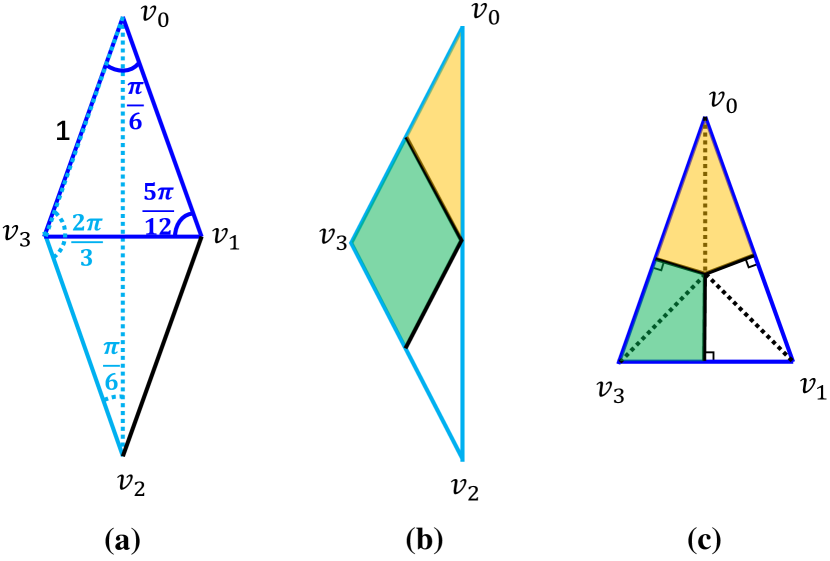
Figure 9: A simple mesh example to show that the original Cotan formula does not guarantee to be positive semidefinite.

Distortion types	Description	Generating details
Impulse	Adding impulsive noise on mesh surface	We add Gaussian noise on $r$ percent of the ground truth mesh vertices. The mean of the Gaussian noise is set to 0 and standard derivation is set to $\sigma$ percent of the mesh scale. For 4 levels of this distortion, ($r$, $\sigma$) are set to (1, 0.5), (5, 2), (8, 3), and (1, 5), respectively.
Poisson reconstruction noise	Synthesizing the noise occurs in Poisson reconstruction [29]	We first use Poisson disk sampling [8] to sample $sN$ points from the groundtruth mesh surface, where $N$ is the number of vertices in groundtruth mesh. Then, we use Poisson reconstruction provided in MeshLab [15] to reconstruct the mesh surface from the sampled points. The reconstruction depth is set to 6. For 4 levels of this distortion, $s$ is set to 0.9, 0.5, 0.2, and 0.05, respectively.
Smoothing	Smoothing mesh surface	We apply $i$ times of $\lambda-\mu$ Taubin smoothing [61] to smooth the groundtruth mesh surface, where $\lambda=0.5$ and $\mu=-0.53$. For 4 levels of this distortion, $i$ is set to 5, 20, 50, and 200, respectively.
Unproportional scaling	Stretching (or shrinking) the mesh along $x$, $y$, and $z$ axis with different rates	We stretch the mesh to $s_{x}$ percent to its original length along $x$ axis, and shrink the mesh to $s_{z}$ percent to its original length along $z$ axis. For 4 levels of this distortion, ($s_{x}$, $s_{z}$) are set to (98, 102), (95, 105), (90, 110), (80, 120), respectively.
Low-resolution mesh	Simplifying mesh surface to lower resolution	We simply the ground truth mesh surface using edge collapse algorithm [21]. For 4 levels of this distortion, the target face number is set to 5000, 2000, 1000, and 500, respectively.
White noise	Adding Gaussian white noise on mesh surface	We add Gaussian noise on all the groundtruth mesh vertices. The mean of the Gaussian noise is set to 0 and standard derivation is set to $\sigma$ percent of the mesh scale. For 4 levels of this distortion, $\sigma$ is set to 0.1, 0.2, 0.3, and 0.5, respectively.
Outlying noise	Adding outlying small floating spheres around the mesh	We add floating spheres around the ground truth mesh to synthesize outlying noise that occurs in 3D reconstruction. The number of the spheres is set to $n$ and the radius $rA$, where $A$ is the maximum length of the mesh along $x$, $y$, and $z$ dimensions. The locations of the spheres are sampled randomly from a cube that surrounds the ground truth mesh. The edge size of the cube is set to $(1+6r)A$. For 4 levels of this distortion, ($n$, $r$) are set to (20, 0.002), (30, 0.004), (40, 0.006), (80, 0.008), respectively.

Table 6: Distortions in our provided Shape Grading dataset.

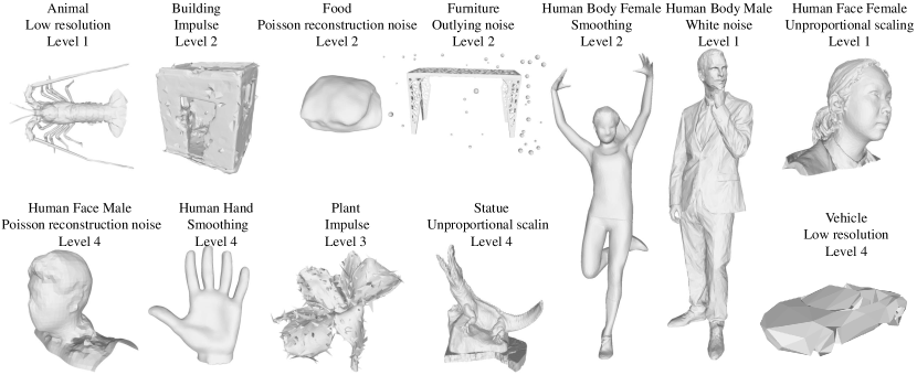
Figure 10: Examples of distorted meshes of different distortion levels in our provided Shape Grading dataset.

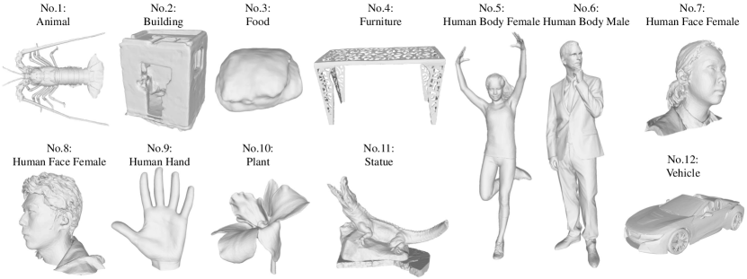
Figure 11: Objects in our provided Shape Grading dataset and what the object numbers correspond to in main paper Table 2.

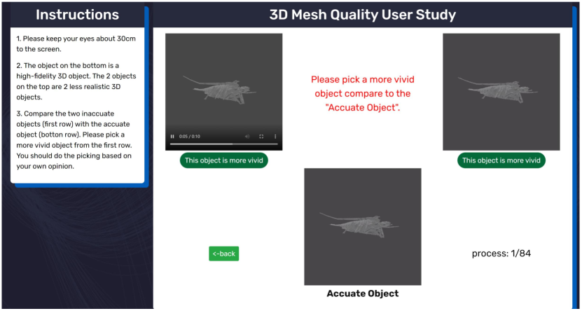
Figure 12: The panel of our online user study system. The instructions on the left contain simple instructions for the subjects. On the right side of the page, the top two videos are rendered from distorted meshes. The lower video is rendered from ground truth mesh.

Appendix C A Counterexample of the Original Cotan Formula not Being Positive Semidefinite

In this section, we provide a simple mesh example to show that the original Cotan formula in main paper Equation (2) does not guarantee to be positive semidefinite. As shown in Fig. 9a, we reconstruct a 4-vertex mesh that is not Delauney triangulated and the mixed Voronoi areas of the vertices are not all equal. We make the two faces on the bottom ($v_{1}v_{2}v_{0}$ and $v_{3}v_{0}v_{2}$) be two congruent obtuse isosceles triangles (shown in Fig. 9b). The apex angles of the two isosceles triangles are $\frac{2\pi}{3}$, and the base angles are $\frac{\pi}{6}$. If we make the bottom two obtuse triangles form different angles to each other, the top two triangle faces ($v_{0}v_{1}v_{3}$ and $v_{2}v_{3}v_{1}$) are always congruent isosceles triangles (as in Fig. 9c), and their apex angles vary continuously in the range of $(0,\frac{\pi}{3})$. Here, we make the bottom two obtuse triangles form a certain angle to each other so that the apex angles of the top two triangles are equal to $\frac{\pi}{6}$, which means their base angles are $\frac{5\pi}{12}$. For simplicity, we set the equal sides of the isosceles triangles to be 1 (shown in Fig. 9a).

Now, we calculate the DLBO metric of this reconstructed mesh using the Cotan formula in main paper Equation (2). First, we calculate the mixed Voronoi area for each vertex. Because of the shape symmetry, we only need to calculate the mixed Voronoi areas for vertex $v_{0}$ and $v_{3}$. The mixed Voronoi areas for vertex $v_{2}$ and $v_{1}$ are equal to $v_{0}$ and $v_{3}$, respectively. For vertex $v_{0}$, its mixed Voronoi area $A_{0}$ can be calculated as the sum of 2 times of yellow area in Fig. 9b and 1 time of yellow area in Fig. 9c, which means

$$\small\begin{split}A_{0}&=2\times(\frac{1}{4}\times\frac{1}{2}\cos\frac{\pi}{3})+1\times(0.5\tan\frac{\pi}{12}\times 0.5)\\ &=\frac{4-\sqrt{3}}{8},\end{split}$$ (30)

where $\frac{1}{2}\cos\frac{\pi}{3}$ is the area of the outer triangle in Fig. 9b and $0.5\tan\frac{\pi}{12}\times 0.5$ is the area of the yellow part in Fig. 9c. For vertex $v_{3}$, its mixed Voronoi area $A_{3}$ can be calculated as the sum of 1 time of green area in Fig. 9b and 2 times of green area in Fig. 9c, which means

$$\small\begin{split}A_{3}&=1\times(\frac{1}{2}\times\frac{1}{2}\cos\frac{\pi}{3})\\ &+2\times(\frac{1}{2}\times(\sin\frac{\pi}{12}\cos\frac{\pi}{12}-0.5\tan\frac{\pi}{12}\times 0.5))\\ &=\frac{3\sqrt{3}-2}{8},\end{split}$$ (31)

where $\sin\frac{\pi}{12}\cos\frac{\pi}{12}$ is the area of the outer triangle in Fig. 9c.

Second, we calculate the DLBO matrix according to main paper Equation (2). The DLBO matrix of the constructed mesh can be represented as

$$L=\left(\begin{array}[]{llll}\frac{w_{1}}{2A_{0}}&\frac{w_{0}}{2A_{0}}&\frac{w_{3}}{2A_{0}}&\frac{w_{0}}{2A_{0}}\\ \frac{w_{0}}{2A_{3}}&\frac{w_{2}}{2A_{3}}&\frac{w_{0}}{2A_{3}}&\frac{w_{4}}{2A_{3}}\\ \frac{w_{3}}{2A_{0}}&\frac{w_{0}}{2A_{0}}&\frac{w_{1}}{2A_{0}}&\frac{w_{0}}{2A_{0}}\\ \frac{w_{0}}{2A_{3}}&\frac{w_{4}}{2A_{3}}&\frac{w_{0}}{2A_{3}}&\frac{w_{2}}{2A_{3}}\par\end{array}\right),$$ (32)

where

$$\begin{split}&w_{0}=-(\cot\frac{5\pi}{12}+\cot\frac{\pi}{6})=-2,\\ &w_{1}=2(\cot\frac{5\pi}{12}+\cot\frac{\pi}{6}+\cot\frac{2\pi}{3})=4-\frac{2\sqrt{3}}{3},\\ &w_{2}=2(\cot\frac{5\pi}{12}+\cot\frac{\pi}{6}+\cot\frac{\pi}{6})=4+2\sqrt{3},\\ &w_{3}=-2\cot\frac{2\pi}{3}=\frac{2\sqrt{3}}{3},\\ &w_{4}=-2\cot\frac{\pi}{6}=-2\sqrt{3}.\end{split}$$ (33)

Then, we can calculate the symmetric part of $L$ as

$$L_{sym}=\frac{L+L^{\top}}{2}.$$ (34)

We use Wolfram Mathematica [67] to calculate the eigenvalues of $L_{sym}$. The 4 eigenvalues are

$$\begin{split}&\lambda_{0}=\frac{2-\frac{2\sqrt{3}}{3}}{A_{0}},\\ &\lambda_{1}=\frac{2+2\sqrt{3}}{A_{3}},\\ &\lambda_{2}=\frac{A_{0}+A_{3}-\sqrt{2(A_{0}^{2}+A_{3}^{2})}}{A_{0}A_{3}},\\ &\lambda_{3}=\frac{A_{0}+A_{3}+\sqrt{2(A_{0}^{2}+A_{3}^{2})}}{A_{0}A_{3}}.\end{split}$$ (35)

It is obvious that when $A_{0}$ and $A_{3}$ are both greater than 0, $\lambda_{0}$, $\lambda_{1}$, and $\lambda_{3}$ will be greater than 0. However, for $\lambda_{2}$, we have

$$\begin{split}\lambda_{2}&=\frac{A_{0}+A_{3}-\sqrt{2(A_{0}^{2}+A_{3}^{2})}}{A_{0}A_{3}}\\ &=\frac{\sqrt{A_{0}^{2}+A_{3}^{2}+2A_{0}A_{3}}-\sqrt{2(A_{0}^{2}+A_{3}^{2})}}{A_{0}A_{3}}\\ &\leq\frac{\sqrt{A_{0}^{2}+A_{3}^{2}+(A_{0}^{2}+A_{3}^{2})}-\sqrt{2(A_{0}^{2}+A_{3}^{2})}}{A_{0}A_{3}}\\ &=0.\end{split}$$ (36)

The equation holds if and only if $A_{0}=A_{3}$. We know from Eq. 30 and Eq. 31 that $A_{0}\neq A_{3}$. Thus, we have

$$\lambda_{2}<0,$$ (37)

which means in the given mesh example, the original Cotan formula is not positive semidefinite.

Appendix D Objects and Distortions in Shape Grading

Fig. 11 shows the objects in our proposed dataset Shape Grading and what the object numbers correspond to in main paper Table 2. We also show the distortion types that we used in our dataset and how we generate them in Tab. 6. Fig. 10 shows examples of distorted meshes of different distortion levels in our dataset.

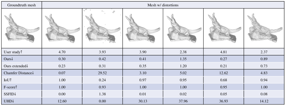
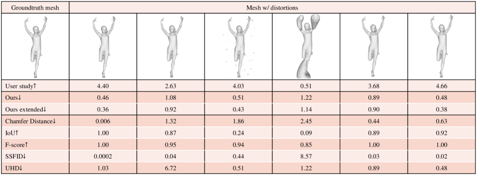
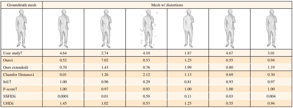
Figure 13: Examples in our dataset and their evaluation results using different metrics. $\downarrow$ means lower is better. $\uparrow$ means higher is better. For each object, the mesh on the top-left is the ground truth mesh, and the rest meshes are distorted meshes. The table below the meshes contains the scores they get from different metrics or from our user study. As shown in the figure, our metric aligns better with user study scores and human perception.

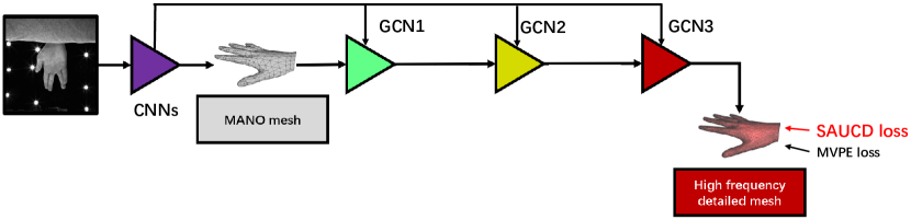
Figure 14: Network architecture used when adapting SAUCD to training loss.

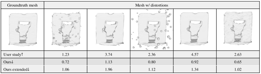
Figure 15: Failure cases. We show a case in which our metric does not provide accurate evaluations aligned with the human evaluation.

Appendix E Swiss System Tournament for Human Scoring

We do a Swiss system tournament for human scoring in main paper Section 4.1. The tournament has 6 rounds. To begin with, all 28 meshes are set to 0 points. In the first round, the 28 meshes are randomly sorted and we form the adjacent meshes into pairs (the 1st and 2nd meshes form a pair, the 3rd and 4th meshes form another pair, etc.). Together, we have 14 pairs. For each pair, we ask the subject which one is closer to the ground truth. The mesh that the subject picked will be added 1 point. From the 2nd to the 6th round, for each round, we first sort the meshes by their current score from low to high, and we also make pairs with adjacent meshes in the sorted mesh array, like what we did in the first round. The mesh closer to ground truth will be added 1 point. The scores of the meshes after 6 rounds are their scores graded by this subject. Fig. 12 shows the panel of our online human scoring page.

Appendix F More Examples and Evaluation Results

We show more examples in our dataset and evaluation results using different metrics in Fig. 13. Compared to previous methods, our provided metrics generally align better with the human evaluation of mesh shape similarity.

Appendix G Implementation Details on Adapting SAUCD to Training Loss

We adapt SAUCD to a topology Laplacian version. Specifically, we replace the Laplacian matrix defined in the main paper Eq.(4) to $L=D-A$ defined in [14], where $D$ is the degree matrix of the mesh graph, and $A$ is the adjacency matrix of the mesh graph. By making the change, we can avoid calculating a different SVD decomposition in every training iteration when mesh vertex locations change. Our network is designed as Fig. 14. The input image first goes through a feature extraction CNNs network to get image features, and uses that feature to generate MANO [51] mesh. Then, we use features from CNNs network and 3 resolution levels of Graph Convolution Networks (GCN) to reconstruct the mesh details. In the main paper Fig. 8, we compare the results using only MVPE loss (w/o SAUCD loss column) and using both MVPE and SAUCD loss (w/ SAUCD loss column). In this experiment, we use EfficientNet [58] and GCN similar to  [31].

Appendix H Failure Cases

We also show a case that our metric does not provide accurate evaluations aligned with the human evaluation in Fig. 15.

Appendix I Discussions of Future Works

In future work, we plan to dig deeper into understanding human sensitivity to frequency changes. To enhance the robustness and applicability of our approach, we plan to expand our dataset to include a wider range of distortions and objects. While our current methods are effective on general 3D meshes, we recognize the importance of developing specialized versions for particular areas of 3D reconstruction, such as human body [23, 24, 38], human face [20, 19], human hand [39], or 3D volumetric approaches [44, 43]. Furthermore, the frequency method holds promise for extension into 2D domains, including the analysis and generation of images  [70, 76, 37, 77, 71, 72], as well as videos [75, 79, 12, 80, 74]. These future works will not only refine our understanding of human perception alignment but also broaden the potential applications of our research in various fields.

References

- [1] Gobotree - photos, cut-outs, 3d people. https://www.gobotree.com/.
- [2] Sketchfab - the best 3d viewer on the web. https://sketchfab.com/.
- Achlioptas et al. [2018] Panos Achlioptas, Olga Diamanti, Ioannis Mitliagkas, and Leonidas Guibas. Learning representations and generative models for 3d point clouds. In ICML, pages 40–49, 2018.
- Bechtold et al. [2021] Jan Bechtold, Maxim Tatarchenko, Volker Fischer, and Thomas Brox. Fostering generalization in single-view 3d reconstruction by learning a hierarchy of local and global shape priors. In CVPR, pages 15880–15889, 2021.
- Blondel et al. [2020] Mathieu Blondel, Olivier Teboul, Quentin Berthet, and Josip Djolonga. Fast differentiable sorting and ranking. In ICML, pages 950–959, 2020.
- Bobenko et al. [2008] Alexander I Bobenko, John M Sullivan, Peter Schröder, and G Ziegler. Discrete differential geometry. Springer, 2008.
- Borgefors [1984] Gunilla Borgefors. Distance transformations in arbitrary dimensions. Computer vision, graphics, and image processing, pages 321–345, 1984.
- Bridson [2007] Robert Bridson. Fast poisson disk sampling in arbitrary dimensions. SIGGRAPH sketches, page 1, 2007.
- BT [2002] RECOMMENDATION ITU-R BT. Methodology for the subjective assessment of the quality of television pictures. International Telecommunication Union, 2002.
- Bulbul et al. [2011] Abdullah Bulbul, Tolga Capin, Guillaume Lavoué, and Marius Preda. Assessing visual quality of 3-d polygonal models. IEEE Signal Processing Magazine, pages 80–90, 2011.
- Burke et al. [1985] William L Burke, William L Burke, and William L Burke. Applied differential geometry. Cambridge University Press, 1985.
- Chen et al. [2022] Hang Chen, Xinyu Yang, and Xiang Li. Learning a general clause-to-clause relationships for enhancing emotion-cause pair extraction. arXiv preprint arXiv:2208.13549, 2022.
- Chen et al. [2021] Zhiqin Chen, Vladimir G Kim, Matthew Fisher, Noam Aigerman, Hao Zhang, and Siddhartha Chaudhuri. Decor-gan: 3d shape detailization by conditional refinement. In CVPR, pages 15740–15749, 2021.
- Chung [1997] Fan RK Chung. Spectral graph theory. American Mathematical Soc., 1997.
- Cignoni et al. [2008] Paolo Cignoni, Marco Callieri, Massimiliano Corsini, Matteo Dellepiane, Fabio Ganovelli, and Guido Ranzuglia. MeshLab: an Open-Source Mesh Processing Tool. In Eurographics Italian Chapter Conference, 2008.
- Corsini et al. [2013] Massimiliano Corsini, Mohamed-Chaker Larabi, Guillaume Lavoué, Oldřich Petřík, Libor Váša, and Kai Wang. Perceptual metrics for static and dynamic triangle meshes. In Comput. Graph. Forum, pages 101–125, 2013.
- Dekking et al. [2005] Frederik Michel Dekking, Cornelis Kraaikamp, Hendrik Paul Lopuhaä, and Ludolf Erwin Meester. A Modern Introduction to Probability and Statistics: Understanding why and how. Springer, 2005.
- Duoandikoetxea and Zuazo [2001] Javier Duoandikoetxea and Javier Duoandikoetxea Zuazo. Fourier analysis. American Mathematical Soc., 2001.
- Gao [2023] Zhongpai Gao. Learning continuous mesh representation with spherical implicit surface. In 2023 IEEE 17th International Conference on Automatic Face and Gesture Recognition (FG), pages 1–8. IEEE, 2023.
- Gao et al. [2020] Zhongpai Gao, Juyong Zhang, Yudong Guo, Chao Ma, Guangtao Zhai, and Xiaokang Yang. Semi-supervised 3d face representation learning from unconstrained photo collections. In CVPRW, pages 348–349, 2020.
- Garland and Heckbert [1997] Michael Garland and Paul S Heckbert. Surface simplification using quadric error metrics. In SIGGRAPH, pages 209–216, 1997.
- Genova et al. [2020] Kyle Genova, Forrester Cole, Avneesh Sud, Aaron Sarna, and Thomas Funkhouser. Local deep implicit functions for 3d shape. In CVPR, pages 4857–4866, 2020.
- Gong et al. [2022] Xuan Gong, Meng Zheng, Benjamin Planche, Srikrishna Karanam, Terrence Chen, David Doermann, and Ziyan Wu. Self-supervised human mesh recovery with cross-representation alignment. In ECCV, pages 212–230, 2022.
- Gong et al. [2023] Xuan Gong, Liangchen Song, Meng Zheng, Benjamin Planche, Terrence Chen, Junsong Yuan, David Doermann, and Ziyan Wu. Progressive multi-view human mesh recovery with self-supervision. In AAAI, pages 676–684, 2023.
- Henderson and Ferrari [2018] Paul Henderson and Vittorio Ferrari. Learning to generate and reconstruct 3d meshes with only 2d supervision. arXiv preprint arXiv:1807.09259, 2018.
- Horn and Johnson [2012] Roger A Horn and Charles R Johnson. Matrix analysis. Cambridge University Press, 2012.
- Hu et al. [2021] Tao Hu, Liwei Wang, Xiaogang Xu, Shu Liu, and Jiaya Jia. Self-supervised 3d mesh reconstruction from single images. In CVPR, pages 6002–6011, 2021.
- Jensen et al. [2014] Rasmus Jensen, Anders Dahl, George Vogiatzis, Engin Tola, and Henrik Aanæs. Large scale multi-view stereopsis evaluation. In CVPR, pages 406–413, 2014.
- Kazhdan et al. [2006] Michael Kazhdan, Matthew Bolitho, and Hugues Hoppe. Poisson surface reconstruction. In Eurographics Symposium on Geometry Processing, 2006.
- Kendall et al. [1946] Maurice George Kendall et al. The advanced theory of statistics. The advanced theory of statistics, 1946.
- Kolotouros et al. [2019] Nikos Kolotouros, Georgios Pavlakos, and Kostas Daniilidis. Convolutional mesh regression for single-image human shape reconstruction. In CVPR, pages 4501–4510, 2019.
- Krishnan and Fergus [2009] Dilip Krishnan and Rob Fergus. Fast image deconvolution using hyper-laplacian priors. NeurIPS, 22, 2009.
- Kulikajevas et al. [2022] Audrius Kulikajevas, Rytis Maskeliunas, Robertas Damasevicius, and Tomas Krilavicius. Auto-refining 3d mesh reconstruction algorithm from limited angle depth data. IEEE Access, pages 87083–87098, 2022.
- Kullback and Leibler [1951] Solomon Kullback and Richard A Leibler. On information and sufficiency. The annals of mathematical statistics, pages 79–86, 1951.
- Lavoué [2009] Guillaume Lavoué. A local roughness measure for 3d meshes and its application to visual masking. ACM Transactions on Applied Perception, pages 1–23, 2009.
- Lin et al. [2022] Peizhen Lin, Hongliang Zhong, Lei Wang, and Jun Cheng. 3d mesh reconstruction of indoor scenes from a single image in-the-wild. In International Conference on Graphics and Image Processing, pages 457–465, 2022.
- Lou et al. [2023] Ange Lou, Kareem Tawfik, Xing Yao, Ziteng Liu, and Jack Noble. Min-max similarity: A contrastive semi-supervised deep learning network for surgical tools segmentation. IEEE TMI, 2023.
- Luan et al. [2021] Tianyu Luan, Yali Wang, Junhao Zhang, Zhe Wang, Zhipeng Zhou, and Yu Qiao. Pc-hmr: Pose calibration for 3d human mesh recovery from 2d images/videos. In AAAI, pages 2269–2276, 2021.
- Luan et al. [2023] Tianyu Luan, Yuanhao Zhai, Jingjing Meng, Zhong Li, Zhang Chen, Yi Xu, and Junsong Yuan. High fidelity 3d hand shape reconstruction via scalable graph frequency decomposition. In CVPR, pages 16795–16804, 2023.
- Meyer et al. [2003] Mark Meyer, Mathieu Desbrun, Peter Schröder, and Alan H Barr. Discrete differential-geometry operators for triangulated 2-manifolds. In Visualization and mathematics III, pages 35–57. Springer, 2003.
- Moon et al. [2020] Gyeongsik Moon, Takaaki Shiratori, and Kyoung Mu Lee. Deephandmesh: A weakly-supervised deep encoder-decoder framework for high-fidelity hand mesh modeling. In ECCV, 2020.
- Nie et al. [2020] Yinyu Nie, Xiaoguang Han, Shihui Guo, Yujian Zheng, Jian Chang, and Jian Jun Zhang. Total3dunderstanding: Joint layout, object pose and mesh reconstruction for indoor scenes from a single image. In CVPR, pages 55–64, 2020.
- Pan et al. [2023a] Shaoyan Pan, Chih-Wei Chang, Marian Axente, Tonghe Wang, Joseph Shelton, Tian Liu, Justin Roper, and Xiaofeng Yang. Data-driven volumetric image generation from surface structures using a patient-specific deep leaning model. arXiv preprint arXiv:2304.14594, 2023a.
- Pan et al. [2023b] Shaoyan Pan, Chih-Wei Chang, Junbo Peng, Jiahan Zhang, Richard LJ Qiu, Tonghe Wang, Justin Roper, Tian Liu, Hui Mao, and Xiaofeng Yang. Cycle-guided denoising diffusion probability model for 3d cross-modality mri synthesis. arXiv preprint arXiv:2305.00042, 2023b.
- Paris et al. [2011] Sylvain Paris, Samuel W Hasinoff, and Jan Kautz. Local laplacian filters: edge-aware image processing with a laplacian pyramid. ACM TOG, page 68, 2011.
- Paszke et al. [2019] Adam Paszke, Sam Gross, Francisco Massa, Adam Lerer, James Bradbury, Gregory Chanan, Trevor Killeen, Zeming Lin, Natalia Gimelshein, Luca Antiga, et al. Pytorch: An imperative style, high-performance deep learning library. NeurIPS, 32, 2019.
- Pearson [1920] Karl Pearson. Notes on the history of correlation. Biometrika, pages 25–45, 1920.
- Pérez et al. [2003] Patrick Pérez, Michel Gangnet, and Andrew Blake. Poisson image editing. In SIGGRAPH, pages 313–318, 2003.
- Ponomarenko et al. [2009] Nikolay Ponomarenko, Vladimir Lukin, Alexander Zelensky, Karen Egiazarian, Marco Carli, and Federica Battisti. Tid2008-a database for evaluation of full-reference visual quality assessment metrics. Advances of Modern Radioelectronics, pages 30–45, 2009.
- Rakotosaona et al. [2021] Marie-Julie Rakotosaona, Paul Guerrero, Noam Aigerman, Niloy J Mitra, and Maks Ovsjanikov. Learning delaunay surface elements for mesh reconstruction. In CVPR, pages 22–31, 2021.
- Romero et al. [2017] Javier Romero, Dimitrios Tzionas, and Michael J. Black. Embodied hands: Modeling and capturing hands and bodies together. SIGGRAPH, 2017.
- Santhanam et al. [2023] Hari Santhanam, Nehal Doiphode, and Jianbo Shi. Automated line labelling: Dataset for contour detection and 3d reconstruction. In WACV, pages 3136–3145, 2023.
- Shen et al. [2007] Jianbing Shen, Xiaogang Jin, Chuan Zhou, and Charlie CL Wang. Gradient based image completion by solving the poisson equation. Computers & Graphics, pages 119–126, 2007.
- Shrestha et al. [2021] Rakesh Shrestha, Zhiwen Fan, Qingkun Su, Zuozhuo Dai, Siyu Zhu, and Ping Tan. Meshmvs: Multi-view stereo guided mesh reconstruction. In 3DV, pages 1290–1300. IEEE, 2021.
- Shu et al. [2019] Dong Wook Shu, Sung Woo Park, and Junseok Kwon. 3d point cloud generative adversarial network based on tree structured graph convolutions. In ICCV, pages 3859–3868, 2019.
- Spearman [1910] Charles Spearman. Correlation calculated from faulty data. British journal of psychology, page 271, 1910.
- Tai and Yang [2008] Shen-Chuan Tai and Shih-Ming Yang. A fast method for image noise estimation using laplacian operator and adaptive edge detection. In International Symposium on Communications, Control and Signal Processing, pages 1077–1081, 2008.
- Tan and Le [2019] Mingxing Tan and Quoc V Le. Efficientnet: Improving accuracy and efficiency through automl and model scaling. arXiv preprint arXiv:1905.11946, 2019.
- Tang et al. [2022] Jiaxiang Tang, Xiaokang Chen, Jingbo Wang, and Gang Zeng. Point scene understanding via disentangled instance mesh reconstruction. In ECCV, pages 684–701, 2022.
- Tatarchenko et al. [2019] Maxim Tatarchenko, Stephan R Richter, René Ranftl, Zhuwen Li, Vladlen Koltun, and Thomas Brox. What do single-view 3d reconstruction networks learn? In CVPR, pages 3405–3414, 2019.
- Taubin [1995] Gabriel Taubin. Curve and surface smoothing without shrinkage. In ICCV, pages 852–857, 1995.
- Wang et al. [2010] Kai Wang, Guillaume Lavoué, Florence Denis, Atilla Baskurt, and Xiyan He. A benchmark for 3d mesh watermarking. In Shape Modeling International Conference, pages 231–235. IEEE, 2010.
- Wang et al. [2022] Lizhen Wang, Zhiyuan Chen, Tao Yu, Chenguang Ma, Liang Li, and Yebin Liu. Faceverse: a fine-grained and detail-controllable 3d face morphable model from a hybrid dataset. In CVPR, pages 20333–20342, 2022.
- Wang et al. [2018] Nanyang Wang, Yinda Zhang, Zhuwen Li, Yanwei Fu, Wei Liu, and Yu-Gang Jiang. Pixel2mesh: Generating 3d mesh models from single rgb images. In ECCV, pages 52–67, 2018.
- Wang [2007] Xin Wang. Laplacian operator-based edge detectors. IEEE TPAMI, pages 886–890, 2007.
- Wei et al. [2021] Xingkui Wei, Zhengqing Chen, Yanwei Fu, Zhaopeng Cui, and Yinda Zhang. Deep hybrid self-prior for full 3d mesh generation. In ICCV, pages 5805–5814, 2021.
- Wolfram [1991] Stephen Wolfram. Mathematica: a system for doing mathematics by computer. Addison Wesley Longman Publishing Co., Inc., 1991.
- Wu and Zheng [2022] Rundi Wu and Changxi Zheng. Learning to generate 3d shapes from a single example. arXiv preprint arXiv:2208.02946, 2022.
- Wu et al. [2020] Rundi Wu, Xuelin Chen, Yixin Zhuang, and Baoquan Chen. Multimodal shape completion via conditional generative adversarial networks. In ECCV, pages 281–296, 2020.
- Xie et al. [2024] Luyuan Xie, Cong Li, Zirui Wang, Xin Zhang, Boyan Chen, Qingni Shen, and Zhonghai Wu. Shisrcnet: Super-resolution and classification network for low-resolution breast cancer histopathology image. MICCAI, 2024.
- Yu et al. [2022] Xin Yu, Qi Yang, Yucheng Tang, Riqiang Gao, Shunxing Bao, Leon Y Cai, Ho Hin Lee, Yuankai Huo, Ann Zenobia Moore, Luigi Ferrucci, et al. Reducing positional variance in cross-sectional abdominal ct slices with deep conditional generative models. In MICCAI, pages 202–212, 2022.
- Yu et al. [2023] Xin Yu, Qi Yang, Yucheng Tang, Riqiang Gao, Shunxing Bao, Leon Y Cai, Ho Hin Lee, Yuankai Huo, Ann Zenobia Moore, Luigi Ferrucci, et al. Deep conditional generative models for longitudinal single-slice abdominal computed tomography harmonization. arXiv preprint arXiv:2309.09392, 2023.
- Zeng et al. [2022] Rongfei Zeng, Mai Su, and Xingwei Wang. Cd2: Fine-grained 3d mesh reconstruction with twice chamfer distance. arXiv preprint arXiv:2206.00447, 2022.
- Zhai et al. [2020] Yuanhao Zhai, Le Wang, Wei Tang, Qilin Zhang, Junsong Yuan, and Gang Hua. Two-stream consensus network for weakly-supervised temporal action localization. In ECCV, pages 37–54, 2020.
- Zhai et al. [2023a] Yuanhao Zhai, Mingzhen Huang, Tianyu Luan, Lu Dong, Ifeoma Nwogu, Siwei Lyu, David Doermann, and Junsong Yuan. Language-guided human motion synthesis with atomic actions. In ACM MM, pages 5262–5271, 2023a.
- Zhai et al. [2023b] Yuanhao Zhai, Tianyu Luan, David Doermann, and Junsong Yuan. Towards generic image manipulation detection with weakly-supervised self-consistency learning. In ICCV, pages 22390–22400, 2023b.
- Zhang et al. [2021] Jiajin Zhang, Hanqing Chao, Xuanang Xu, Chuang Niu, Ge Wang, and Pingkun Yan. Task-oriented low-dose ct image denoising. In MICCAI, pages 441–450, 2021.
- Zhang et al. [2023] Zhihao Zhang, Xinyang Ren, and Xianqiang Yang. Parametric chamfer alignment based on mesh deformation. Measurement and Control, pages 192–201, 2023.
- Zhu et al. [2021] Zixin Zhu, Wei Tang, Le Wang, Nanning Zheng, and Gang Hua. Enriching local and global contexts for temporal action localization. In ICCV, pages 13516–13525, 2021.
- Zhu et al. [2022] Zixin Zhu, Le Wang, Wei Tang, Ziyi Liu, Nanning Zheng, and Gang Hua. Learning disentangled classification and localization representations for temporal action localization. In AAAI, pages 3644–3652, 2022.
- Zuo et al. [2021] Xinxin Zuo, Sen Wang, Minglun Gong, and Li Cheng. Unsupervised 3d human mesh recovery from noisy point clouds. arXiv preprint arXiv:2107.07539, 2021.