Generalized Ghost Dark Energy in Gravity
Abstract
In this manuscript, we use the correspondence principle to construct the generalized ghost dark energy model, where is the non-metricity. For this purpose, we use the Friedman-Robertson-Walker universe model with power-law scale factor. The energy density in this model linearly depends on the Hubble parameter, with a sub-leading term of , resulting in an energy density , where and are arbitrary constants. We reconstruct interacting fluid scenario of this dark energy with dark matter. The reformulated gravity model shows how different epochs of the cosmic history can be reproduced by this modified gravity model. The physical characteristics of the model are discussed through the equation of state parameter with the planes of and . We also explore the stability criteria for the interacting model using the squared speed of sound. The equation of state parameter indicates phantom phase of the universe and the squared speed of sound represents stability of the interacting model. The -plane indicates freezing region, while the -plane corresponds to the Chaplygin gas. We conclude that our findings coincide with the latest observational data.
Keywords: gravity, Generalized ghost dark energy,
Cosmological evolution.
PACS: 04.50.Kd; 95.36.+x; 64.30.+t.
1 Introduction
General relativity (GR) is a theory of gravitation proposed by Albert Einstein and is the most significant discovery of the 20th century. This theory stands as Einstein remarkable scientific legacy, providing a successful framework to unravel the mysteries of our universe evolution and its concealed truths. Recent observations indicate strong evidence about the universe accelerated expansion phase [1]. These observations provide that of the universe contains dark energy (DE) and dark matter (DM) but only of baryonic matter [2]. The expanding universe is said to be the result of exotic force with a large negative pressure, known as DE. The cosmological constant in GR explains the expanding universe but it has two fundamental problems like coincidence and fine tuning. There are two main suggestions to investigate the expanding nature, dynamical DE models and modified theories(MT).
The most fundamental variation of GR is the theory, which is derived from the Einstein-Hilbert(EH) action, by replacing the Ricci scalar with an arbitrary function [3]. Nojiri and Odintsov [4] established modified Gauss-Bonnet theory, termed as gravity, by introducing the generic function into the EH action, where is the Gauss-Bonnet invariant. In particular, realistic models of gravity have been formulated for the observed cosmic accelerated expansion in the late-time universe. The same authors [5] examined various types of modified gravitational theories, including and gravity theories, which are considered alternative theories for DE. They revealed that certain theories within this category could successfully pass the solar system tests and exhibit a robust cosmological structure. The theory of gravity represents another extension of GR, in which represents trace of the energy-momentum tensor (EMT) [6]. Katirci and Kavuk [7] made modifications to the theory by incorporating a non-linear term () within the functional action, leading to what is termed as theory. Sharif and Ikram [8] proposed the inclusion of a generalized function into the EH action to establish gravity. They examined energy conditions within the framework of the FRW universe.
The general theory of relativity is a geometric theory associated with Riemann space. There is another approach to obtain generalized theories of gravity with a more general geometric structure which can describe the gravitational field. Weyl [9] developed a more general geometry than Riemannian by introducing an additional connection (length connection), which does not provide information regarding the direction of the vector during parallel transport. In this theory, the metric tensor’s covariant divergence is non-zero, which yields a novel geometric quantity is non-metricity. Dirac [10] generalized Weyl theory on the basis of two metrics but it was ignored by physicists. Cartan [11] made a significant advancement in geometric theories, giving rise to a new generalized geometric theory is Einstein-Cartan theory [12]. The Weyl geometry can be modified by incorporating torsion, dubbed as Weyl-Cartan geometry [13]. Weitzenbck [14] suggested another mathematical development (Weitzenbck spaces), whose characteristics are , and , where the metric, torsion and curvature tensors are represented by , and , respectively. The Weitzenbck manifold transforms into a Euclidean manifold when . These geometries possess the crucial characteristic of distant parallelism, referred to as absolute parallelism, or tele parallelism.
In the teleparallel theory of gravity, the metric tensor is replaced with a collection of tetrad vectors. Consequently, the torsion is used to characterize gravitational effects instead of the curvature. This gives the teleparallel equivalent to GR, named as theory, where denotes the torsion scalar [15]. Haghani et al. [16] expanded the teleparallel gravity theory into what is known as Weyl-Cartan-Weitzenbck gravity. The same authors [17] proposed another extension of the Weyl-Cartan-Weitzenbck and teleparallel gravity by incorporating the condition of vanishing curvature and torsion in a Weyl-Cartan geometry. The field equations in the gravity theory are of second order, compared to the gravity theory, which is a fourth order theory when examined through a metric approach. The second-order nature of gravity theory has a significant benefit. This discussion leads to the fact that GR can be geometrically divided into two equivalent ways: the curvature description (both the non-metricity and torsion vanish) and the teleparallel description (both the non-metricity and curvature vanish). A third equivalent description is when the non-metricity in the metric signifies the change in vector length during parallel transport. This acts as the fundamental geometric variable characterizing the gravitational interaction properties, leading to symmetric teleparallel gravity (STG), which is also known as theory [18]. There is a great body of literature available [19] to discuss different geometrical and physical aspects of this theory.
The non-metricity is a mathematical concept that emerges in theories involving non-Riemannian geometries, providing an alternative cosmic model without DE. Researchers have drawn attention to explore non-Riemannian geometry, specifically theory, for various reasons such as its theoretical implications, compatibility with observational data and its significance in cosmological contexts [20]. Recent investigations into gravity have revealed cosmic issues and observational constraints can be employed to indicate deviations from the CDM model [21]. The non-metricity scalar has been employed to detect the effects of microscopic systems in [22]. Barros et al. [23] analyzed the cosmic characteristics through redshift space distortion data in non-metricity gravity. For further details, we refer the readers to [24]-[29].
The use of instabilities in quantum field theory suggest that the model may not be well-behaved at the quantum level. Unstable models can lead to inconsistencies when quantum effects are considered. Despite such issues with ghost models, several researchers are interested to explore GDE models for some other well-known motivations. Comparing the predictions of GDE models with standard models allows scientists to understand the differences and potential observable effects. In summary, the use of GDE models in theory is a topic of theoretical exploration, but their realistic viability and compatibility with quantum field theory must be scrutinized to ensure a meaningful contribution to our understanding of cosmology.
The Veneziano GDE has been suggested [30] which is non-physical in the standard Minkowski spacetime but has significant physical consequences in non-trivial topological or dynamical spacetimes. It produces a small vacuum energy density in curved spacetime proportional to and is the quantum chromodynamics mass scale. Therefore, no further changes, degrees of freedom, or parameters are needed. For and , the measured DE density can be accurately ordered by . This remarkable coincidence suggests that the fine-tuning issues are removed by this model [31].
To address the issue of DE, cosmologists have proposed various DE models, including phantom, tachyon, quintessence and Chaplygin gas in different eras. These evolutionary models trace its roots back to the GDE within the Veneziano field of QCD theory. In recent years, this dynamic model has attracted significant attention due to the interesting characteristics of Veneziano GDE, which may be responsible for the current accelerated expansion. Cai et al. [32] explored the Veneziano GDE contribution to the vacuum energy density, demonstrating that it is not completely dependent on . Instead, an additional sub-leading term of must be included in the energy density expression, results in the generalized GDE (GGDE) model, designed to examine the early stages of expansion. In this theoretical framework, the Veneziano ghost maintains compliance with fundamental principles attributes of renormalizable quantum field theory, avoiding any violations of these essential aspects.
Sheykhi and Movahed [33] investigated the consequences of the interacting GDE model within the framework of GR. They analyzed the universe expansion by applying constraints to the model parameters. Setare et al. [34] introduced the interacting DE model within the context of Horava-Lifshitz cosmology. Khodam et al. [35] examined the reconstruction of gravity within the context of the GGDE model. They also investigated the cosmic evolution by analyzing various cosmological parameters. Ebrahimi et al. [36] examined the interacting GGDE in a non-flat universe, discovering that the EoS parameter resides in the phantom era of the universe. Sharif and Jawad [37] analyzed the dynamics of interacting pilgrim DE models using standard cosmological parameters. Additionally, they assessed the stability of the DE model within the context of the FRW universe model. Ebrahimi and Sheykhi [38] proposed the detection of instability signals from generalized quantum chromodynamics GDE. Pasqua et al. [39] studied DE at a higher order of in the context of gravity. Their findings revealed that the model demonstrates stability in the early universe but becomes unstable in the current era.
Sharif and Zubair [40] applied the statefinder diagnostic to both the phantom and quintom DE models. Jawad and Rani [41] investigated the reconstruction of generalized ghost pilgrim DE in the context of gravity. Sharif and Nawazish [42] investigated the interacting and non-interacting DE models in gravity. Sharif and Saba [43] studied the cosmography of GGDE in and gravity theories. Lu, Zhao and Chee [44] studied the cosmic characteristics in symmetric teleparallel gravity (STG), revealing that the accelerating expansion is an inherent property of the universe’s geometry. Lazkoz et al. [45] investigated observational constraints of gravity. Mandal et al. [46] analyzed limitations on the Hubble constant and the cosmographic functions in this theory. Shekh [47] studied the dynamical investigation of holographic DE models in the context of this theory. Mandal et al. [48] calculated the value of equation of state (EoS) parameter for Pantheon samples as well as Hubble parameter. The result of model shows quintessential behavior that diverges from the standard cold DM. Lymperis [49] investigated the cosmological implications through the effective DE sector in the same theory. Solanki et al. [50] discovered that the geometric extension of GR could serve as a viable candidate for explaining the origin of DE. Recently, the parametrization of the effective EoS parameter in this framework has been explored in [51].
This paper reconstructs the GGDE model in the interacting case using the correspondence scheme. We investigate evolution of the universe using the EoS parameter, the squared speed of sound () and phase planes. We organize the article in the following pattern. Section 2 presents the description of this MT of gravity. In section 3, we discuss the effects of interacting DE and CDM in terms of red-shift parameter and apply a correspondence technique between GGDE and gravity to reconstruct GGDE model. Section 4 is dedicated to explore the evolution of this model through cosmographic analysis. Section 5 provides the summary of our results.
2 Brief Sketch of Theory
This segment briefly reviews the geometrical structure of the MT of gravity on the basis of the spacetime. We use the variational principle to formulate the field equations of the theory.
2.1 Geometrical Foundation
Weyl [9] extended the Riemannian geometry (basis of GR) by assuming that an arbitrary vector will change both its direction as well as length during the parallel transport around a closed path. The resultant geometric theory exhibits mathematical properties with the vector that are identical to those of electromagnetic potentials. This implies that there might be a shared geometric origin for both electromagnetic and gravitational forces [15].
In a Weyl space, when a vector of length is parallel transported along a very small path, say , the change in its length is given by . However, for a vector with a small closed loop of area (, its length variation is , where
| (1) |
and is the usual covariant derivative. A local scaling length represented as induces a transformation in the vector field to , where the metric components are transformed by the conformal transformations and .
| (2) |
where is the Christoffel symbol. In Weyl geometry, is symmetric in its lower indices [52] which helps to evaluate gauge covariant derivative. The Weyl curvature tensor can be found through the covariant derivative as
| (3) |
where
| (4) | |||||
| (5) | |||||
The contraction of the Weyl curvature tensor gives
| (6) |
where is the Ricci tensor and the Weyl scalar is
| (7) |
A generalization of the Weyl geometry with torsion yields the Weyl-Cartan (WC) spaces. In this spacetime, one can define a symmetric metric tensor and an asymmetric connection [53], where the torsion tensor can be written as
| (8) |
Here, is the contortion tensor, is the disformation tensor and the Levi-Civita connection is expressed as
| (9) |
The contortion tensor is defined as
| (10) |
which is antisymmetric and . The non-metricity yields the disformation tensor as
| (11) |
As the negative covariant derivative of the metric tensor with WC connection is expressed as , the non-metricity tensor can be obtained
| (12) |
By comparing Eqs.(2) and (8), we can deduce that Weyl geometry is a specific instance of WC geometry when the torsion is zero, and . Consequently, the connection in WC geometry can be expressed as
| (13) |
where
| (14) |
The WC torsion is described as
| (15) |
and the WC curvature tensor as
| (16) |
We can calculate in terms of the Riemann tensor using Eq.(13) as
| (17) | |||||
where , and the covariant derivative is calculated in relation to the metric tensor.
In the framework of symmetric connection, the Levi-Civita connection can be represented in relation to the disformation tensor as
| (18) |
It is well-known from GR that the gravitational action can be restated in a non-covariant form after removing the boundary terms from the Ricci scalar as
| (19) |
Using Eq.(18), the gravitational action (in the coincident gauge) in terms of the disformation tensor becomes
| (20) |
This is the action of the STG with some basic differences between the actions of GR and STG. Firstly, the curvature tensor vanishes in the STG, thus the overall geometry is characterized by flatness and it turns out to be Weitzenbck type geometry [54]. Secondly, the gravitational effects arising from the variations in the length of the vector instead of the rotation of the angle between two vectors during parallel transport.
2.2 The Field Equations of Gravity
Here, we examine an extension of the STG Lagrangian (20) as
| (21) |
where, determinant of the metric tensor and matter-Lagrangian density are represented by and , respectively. The non-metricity scalar is defined as
| (22) |
while Eq.(18) gives
| (23) |
The trace of the tensor is given as
| (24) |
The superpotential is defined as a function of the tensor as
| (25) |
Consequently, the relation for becomes (details are given in Appendix A)
| (26) |
The field equations can be obtained by taking the variation of with respect to the metric tensor as zero
| (27) | |||||
where we have used Appendix B. Using the EMT
| (28) |
and , the field equations of gravity take the form
| (29) |
where .
In theoretical cosmology, the most crucial challenge is to comprehend and regulate the cosmic expansion during both the early as well as late stages. The idea of modifying matter or gravity has attracted a great deal of attention. This noteworthy concept of theoretical advancements, including higher-order gravitational theories, encompass anti-gravity effects arising from higher-order curvature terms. A significant advantage of the gravity theory lies in the fact that its field equations are of second order. Within this framework, the gravitational field is characterized by the function of non-metricity scalar . Non-metricity is a geometric quantity related to the deviation from metric compatibility in the theory of connections. The specific form of the function determines the gravitational dynamics. This theory involves non-metricity scalar, introducing additional geometric structures beyond the metric tensor. We have employed a recently introduced GGDE model, characterized by a strong repulsive force that prevents the formation of black holes. These models stand out as significant solutions to the recent cosmic acceleration problem.
3 Reconstruction of GGDE Model
To reconstruct the GGDE model, we use a correspondence technique between GGDE and gravity in this section. The line element of spatially homogeneous and isotropic universe model is given by
| (30) |
where the scale factor is denoted by . The EMT for perfect fluid configuration containing four velocity field , the usual matter density and pressure and , respectively, is given as
| (31) |
The modified Friedman equations for gravity are
| (32) |
here dot means derivative with respect to time while and are the DE density and pressure, respectively, given by
| (33) | |||||
| (34) |
The two fractional energy densities and are given as follows
| (35) |
implying that , where is the critical density. Consider the interaction between two fluids, i.e., the DE and dark matter. Therefore, the continuity of two fluids yields that the energy densities of the two fluids do not conserve separately but takes the following form for the interacting case
| (36) |
here, represents the interaction term. It is evident that must be positive, signifying the occurrence of energy transfer from DE to DM. Since the unit of is the inverse of time evolution, it is natural to choose this value as the product of and . In this context, we examine , where denotes the coupling constant, representing the transfer strength from DE to DM and is given as
| (37) |
With the parameters defined above, we can write as
| (38) |
Dynamical DE models involving energy density proportional to the Hubble parameter are essential to explain the accelerated expansion of the universe. In this scenario, the GGDE model is a dynamical DE model possessing energy density as The energy density for GGDE model can be expressed as
| (39) |
The theory has successfully undergone observational tests within the confines of the solar system [55]. Considering the dynamic behavior of the GGDE model, it is more appropriate to analyze this model within a dynamic framework, such as the theory. It has been demonstrated that certain characteristics of the original GDE in cosmology deviate from GR. A phenomenological model of GGDE was recently introduced, characterized by an energy density expressed as . This model aims to provide an explanation for the observed acceleration of the universe expansion. The subleading term can induce delays in various epochs of cosmic evolution. The GGDE model mimics the behavior of cosmological constant. It is noteworthy that this behavior is consistent with that of the original GDE model. This is expected, as the in the late time can be neglected due to the smallness of , and the distinction between these two models becomes apparent only in the early epochs of the universe. The solution of the Friedman equations of our model leads to a stable universe in theory due to non-metricity factor .
By equating the associated densities, we establish the relationship between GGDE and the gravity model [32]. Using Eqs.(33) and (39), it is obvious that
| (40) |
which can also be written as
| (41) |
The represents the first-order linear differential equation in terms of whose solution is
| (42) |
where and are integration constants. This is the reconstructed GGDE model in gravity.
Now, we write down this solution in terms of the redshift parameter. We express the scale factor in the form of a power law, given by
| (43) |
where is an arbitrary constant whose current value is and is an arbitrary constant. The deceleration parameter is defined as
| (44) |
When , it represents that the universe is accelerating while indicates deceleration. Substituting the value of in Eq.(43), we obtain
| (45) |
where represents the expanding universe. Moreover, the current universe is accelerating, as indicated by the current value of the deceleration parameter, i.e., [56]. The historical expansion and the current expansion rates of the universe can be expressed as
| (46) |
This indicates that the parameters and determine the cosmic expansion. Using the relationship between the scale factor and the redshift parameter , we have
| (47) |
where .
One can calculate as (details are given in Appendix B). Using the value of , we have
| (48) |
Inserting this value in Eq.(42), the solution in terms of redshift parameter can be written as
| (49) |
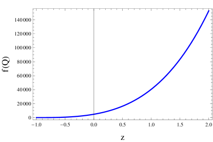
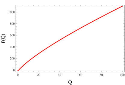
We take throughout the graphical analysis. Figure 1 shows that the reconstructed GGDE model maintains positive value and increases with respect to both as well as . This analysis suggests that the GGDE model signifies an accelerated expansion. We also note that our reconstructed model approaches to zero when tends to zero which implies a realistic behavior of the resulting model.

Next, we investigate the behavior of and for the reconstructed GGDE gravity model. Using Eq.(42) in (33) and (34), it follows that
| (50) | |||||
| (51) | |||||
Converting these equations in terms of redshift parameter, we have
| (52) |
| (53) | |||||
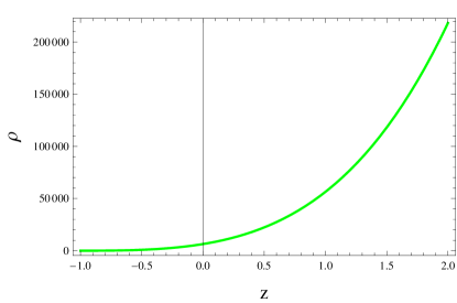
Figures 2 shows the behavior of and with redshift parameter. The energy density maintains positive behavior and increases, while the maintains negative behavior and exhibits a decreasing trend for all which is consistent with the DE behavior.
4 Cosmographic Analysis
In this section, we investigate cosmic evolution through cosmographic analysis of the EoS parameter and phase planes for the reconstructed GGDE model in the interacting case. We also discuss the stability of this model by considering .
4.1 Equation of State Parameter
In the field of cosmology, the EoS parameter () can be classified into various phases of the cosmic evolution. The values of indicate the matter-dominated regions, i.e., dust, radiation and stiff matter, respectively. For the DE era, lead to vacuum, phantom and quintessence phases of the universe expansion. Using Eq.(38), we have
| (54) | |||||
This equation in terms of the redshift parameter becomes
| (55) | |||||
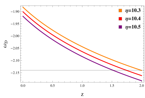
Figure 3 illustrates the dynamic evolution of the EoS in the GGDE gravity model for three different values of . This indicates that in the late universe (), yielding a phantom field DE. This phantom phase is maintained for , whereas this represents a quintessence phase () for .
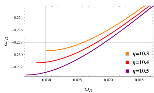
4.2 The ()-Plane
Caldwell and Eric [57] examined the behavior of quintessence scalar field DE models. They analyzed the -plane, where represents the rate of change or evolution of with respect to . We can categorize the models into two distinct classes, i.e., thawing and freezing regions. The thawing region is characterized by , while the freezing region by . Differentiating Eq. (54) with respect to , we get
In terms of redshift parameter, this takes the form
| (56) | |||||
Figure 4 shows that for all values of , which ensures the presence of the freezing region. This indicates that the cosmological expansion is accelerating at a higher rate within this framework.
Here, we utilize the -plane in order to illustrate the current cosmic expansion paradigm. In our work, behavior of the -plane represents freezing region in interacting GGDE model within the framework of gravity. However, the result depicts that -plane represents thawing region which is less accelerating phase as compared with freezing region in gravity [43].
4.3 The -Plane
Sahni et al. [58] presented a set of dimensionless parameters , which are referred to as the statefinder parameters. These are characterized as [59]
In this scenario, the universe comprises two distinct components of the EoS parameter: the usual matter represented by and an exotic form of energy denoted as . The parameters can be defined as [59]
These are helpful in distinguishing various DE models of the cosmos and also give distance of a particular DE model through lambda cold dark matter limit. The literature indicates CDM limit for and lambda CDM limit for . When the trajectories of the plane lie in the range of , we have phantom and quintessence DE eras and for the range , we obtain Chaplygin gas model. The diagnostic in terms of redshift parameter are given as follows
| (57) | |||||
| (58) | |||||
Figure 5 shows that , indicating Chaplygin gas model for . When , the trajectories of the plane lie in the range of , indicating phantom and quintessence DE eras and for , the trajectories lie in the range of , indicating Chaplygin gas model.
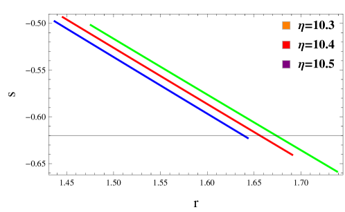
The acceleration of cosmic expansion is specified by parameter s whereas the deviation from pure power-law behavior is specifically defined by the parameter . It is a geometric diagnostic that does not support any specific cosmological paradigm. Furthermore, it attains CDM limit but can not achieve limit. We have observed that, for a significant portion, the plane results in the phantom region in the context of the Chaplygin gas model. Furthermore, our reconstructed model, within the framework of an interacting scenario, attains the CDM limit. This is in contrast to the correspondence between and GGDE model. Our results are consistent with these cosmos [43].
4.4 The Squared Speed of Sound Parameter
To assess the stability of the DE model, perturbation theory offers a direct analysis by examining the sign of the . When is negative, perturbations intensify, leading to an unstable state. Conversely, if is positive, perturbations exhibit oscillatory behavior, suggesting the stability of the background in the presence of linear disturbances. The corresponding is given as
In terms of redshift parameter, it becomes
| (59) | |||||
Figure 6 demonstrates a positively increasing trajectory of , implying the stability of GGDE model for all values of .
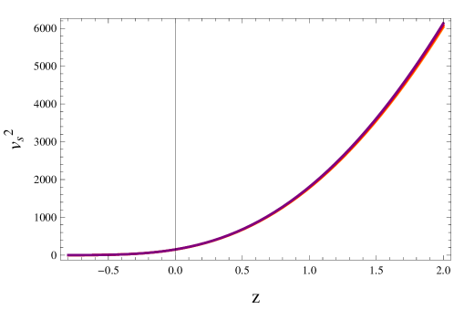
Stability analysis is used to investigate the conditions under which cosmic formations maintain their stability in the presence of various oscillation patterns. The squared speed of sound determines the rate at which pressure waves travel through a medium. Its signature plays a crucial role in discussing the stability of the reconstructed GGDE model. Here, it is worth highlighting that we have achieved increased stability behavior, thanks to the inclusion of non-metricity, in contrast to both GR and other MT. It is also noted that certain characteristics of the original GDE in cosmology differ from those in GR.
5 Conclusions
The phenomena of reconstruction in MT of gravity provides a helpful instrument for creating a workable DE model that predicts the course of cosmic progress. In this situation, we evaluate and contrast the respective energy densities of DE and MT. This enables the correspondence technique to lead to the required generic function of underlying gravity theory. Many researchers have employed this scheme to derive feasible DE models. In this paper, we have studied the GGDE model in gravity. Firstly, we have reconstructed the GGDE gravity model using the correspondence scheme. We have used FRW model with power-law form of the scale factor for the interacting case. We have then examined the evolution trajectories of the EoS, the and -planes. Finally, we have explored the solutions of the DE model . The main results are given as follows.
-
•
The resulting GGDE gravity model demonstrates an increasing trend for both as well as , signifying the realistic nature of the reconstructed model (Figure 1).
-
•
The energy density exhibits positive behavior and increases, while the pressure displays negative behavior. This behavior coincides with the characteristics of DE (Figure 2).
-
•
We have found that the EoS characterizes the late universe involving phantom field DE. We have also observed that the EoS takes more negative values below as the interaction parameter increases (Figure 3). Our findings thus support the present accelerated cosmic behavior.
-
•
The evolutionary behavior of (-)-plane represents the freezing region for all values of (Figure 4). This confirms that the interacting GGDE gravity model implies more accelerated expanding universe.
-
•
The -plane represents Chaplygin gas model for different values of (Figure 5).
-
•
We have found that the is positive and hence GGDE gravity model is stable for all values of (Figure 6).
We have observed that the GGDE model demonstrates stable characteristics and maintains consistent behavior with the current accelerated expansion paradigm of the universe. The phantom-like behavior of the cosmos is noted to anticipate a more accelerated regime, which might ultimately lead to the big-rip scenario or the universe’s present accelerated condition. We noticed that the results are consistent with the current observational data [60] given as
These values have been determined through the application of various observational techniques at a 95% confidence level. It is noteworthy to mention here that our results coincide with the findings from the reconstructed quantum chromodynamics ghost model in gravity [61] and the theory [62]. We would like to emphasize that our results coincide with the latest theoretical observational data examined by Myrzakulov et al. [59].
Appendix A: Calculation of
Appendix B: Evaluation of
Appendix C: Computation of
References
- [1] A.G. Riess, A.V. Filippenko, P. Challis, Supernova search team, Astron. J. 116 (1998) 1009; S. Perlmutter, et al., Measurements of and from 42 high-redshift supernovae, Astrophys. J. 517 (1999) 565; P. de Bernardis, et al., A flat Universe from high-resolution maps of the cosmic microwave background radiation, Nature 404 (2000) 955; A.G. Riess, et al., A 3% solution: determination of the Hubble constant with the Hubble Space Telescope and Wide Field Camera 3, Astrophys. J. 730 (2011) 119; P.A. Ade, et al., Planck 2015 results-xiii. cosmological parameters, Astron. Astrophys. 594 (2016) A13.
- [2] P.J.E. Peebles, B. Ratra, The cosmological constant and dark energy, Rev. Mod. Phys. 75 (2003) 559; T. Padmanabhan, Cosmological constant-the weight of the vacuum, Phys. Rep. 380 (2003) 235; G. Cognola, et al., Class of viable modified gravities describing inflation and the onset of accelerated expansion, Phys. Rev. D 77 (2008) 046009.
- [3] H.A. Buchdahl, Non-linear Lagrangians and cosmological theory, Month. Not. R. Astron. Soc. 150 (1970) 1; J.D. Barrow, A.C. Ottewill, The stability of general relativistic cosmological theory, J. Phys. A: Math. Gen. 16 (1983) 2757.
- [4] S. Nojiri, S.D. Odintsov, Modified Gauss-Bonnet theory as gravitational alternative for dark energy, Phys. Lett. B 631 (2005) 1.
- [5] S. Nojiri, S.D. Odintsov, Introduction to modified gravity and gravitational alternative for dark energy, Int. J. Geom. Methods Mod. Phys. 4 (2007) 115.
- [6] O. Bertolami, C.G. Boehmer, T. Harko, F.S. Lobo, Extra force in modified theories of gravity, Phys. Rev. D 75 (2007) 104016.
- [7] N. Katirci, M. Kavuk, gravity and Cardassian-like expansion as one of its consequences, Eur. Phys. J. Plus 129 (2014) 163.
- [8] M. Sharif, A. Ikram, Energy conditions in gravity, Eur. Phys. J. C 76 (2016) 640.
- [9] H. Weyl, Gravitation und elektrizitt, Sitzungsber. Preuss. Akad. Wiss. 465 (1918) 01.
- [10] P.A.M. Dirac, Long range forces and broken symmetries, Proc. R. Soc. London A 333 (1973) 403.
- [11] . Cartan, Sur unegnralisation de la notion de courbure de Riemann et les espaces torsion, C.R. and Acad. Sci. Paris 174 (1922) 593.
- [12] F.W. Hehl, P. Von der Heyde, G.D. Kerlick, J.M. Nester, General relativity with spin and torsion: Foundations and prospects, Rev. Mod. Phys. 48 (1976) 393.
- [13] M. Novello, S.P. Bergliaffa, Bouncing cosmologies, Phys. Rep. 463 (2008) 127.
- [14] R. Weitzenbck, N. Invariantentheorie, Groningen, The Netherlands, 1923.
- [15] K. Hayashi, T. Shirafuji, New general relativity, Phys. Rev. D 19 (1979) 3524; R. Aldrovandi, J.G. Pereira, Teleparallel gravity: An introduction, Springer, 2013.
- [16] Z. Haghani, T. Harko, H.R. Sepangi, S. Shahidi, Weyl-Cartan-Weitzenbck gravity as a generalization of teleparallel gravity, J. Cosm. AstroPhys. 10 (2012) 061.
- [17] Z. Haghani, T. Harko, H.R. Sepangi, S. Shahidi, Weyl-Cartan-Weitzenbck gravity through Lagrange multiplier, Phys. Rev. D 88 (2013) 044024.
- [18] J.B. Jimnez, L. Heisenberg, T. Koivisto, Coincident general relativity, Phys. Rev. D 98 (2018) 044048.
- [19] A. Conroy, T. Koivisto, The spectrum of symmetric teleparallel gravity, Eur. Phys. J. C 78 (2018) 923; L. Jrv, M. Rnkla, M. Saal, O. Vilson, Nonmetricity formulation of general relativity and its scalar-tensor extension, Phys. Rev. D 97 (2018) 124025; A. Delhom-Latorre, G.J. Olmo, M. Ronco, Observable traces of non-metricity: new constraints on metric-affine gravity, Phys. Lett. B 780 (2018) 294; T. Harko, et al., Coupling matter in modified gravity, Phys. Rev. D 98 (2018) 084043; M. Hohmann, C. Pfeifer, U. Ualikhanova, J.L. Said, Propagation of gravitational waves in symmetric teleparallel gravity theories, Phys. Rev. D 99 (2019) 024009; J. Lu, X. Zhao, G. Chee, Cosmology in symmetric teleparallel gravity and its dynamical system, Eur. Phys. J. C 79 (2019) 530.
- [20] J.B. Jimnez, L. Heisenberg, T. Koivisto, S. Pekar, Cosmology in geometry, Phys. Rev. D 101 (2020) 103507.
- [21] J. Lu, X. Zhao, G. Chee, Cosmology in symmetric teleparallel gravity and its dynamical system, Eur. Phys. J. C 79 (2019) 530; F.K. Anagnostopoulos, S. Basilakos, E.N. Saridakis, First evidence that non-metricity gravity could challenge CDM, Phys. Lett. B 822 (2021) 136634.
- [22] W. Wang, H. Chen, T. Katsuragawa, Static and spherically symmetric solutions in gravity, Phys. Rev. D 105 (2022) 024060.
- [23] K.F. Dialektopoulos, T.S. Koivisto, S. Capozziello, Noether symmetries in symmetric teleparallel cosmology, Eur. Phys. J. C 79 (2019) 606.
- [24] F. Ambrosio, M. Garg, L. Heisenberg, Non-linear extension of non-metricity scalar for MOND, Phys. Lett. B 811 (2020) 135970.
- [25] I. Ayuso, R. Lazkoz, V. Salzano, Observational constraints on cosmological solutions of theories, Phys. Rev. D 103 (2021) 063505.
- [26] K. Flathmann, M. Hohmann, Post-Newtonian limit of generalized symmetric teleparallel gravity, Phys. Rev. D 103 (2021) 044030.
- [27] N. Frusciante, Signatures of gravity in cosmology, Phys. Rev. D 103 (2021) 044021.
- [28] W. Khyllep, A. Paliathanasis, J. Dutta, Cosmological solutions and growth index of matter perturbations in gravity, Phys. Rev. D 103 (2021) 103521.
- [29] S. Capozziello, R. Agostino, Model-independent reconstruction of non-metric gravity, Phys. Lett. B 832 (2022) 137229.
- [30] F.R. Urban, A.R. Zhitnitsky, Cosmological constant from the ghost: a toy model, Phys. Rev. D 80 (2009) 063001.
- [31] N. Ohta, Dark energy and QCD ghost, Int. J. Mod. Phys. Conf. Ser. 7 (2012) 194. World Scientific Publishing Company.
- [32] R.G. Cai, Z.L. Tuo, Y.B. Wu, Y.Y. Zhao, More on QCD ghost dark energy, Phys. Rev. D 86 (2012) 023511.
- [33] A. Sheykhi, M.S. Movahed, Interacting ghost dark energy in non-flat universe, Gen. Relativ. Gravit. 44 (2012) 449.
- [34] M.R. Setare, D. Momeni, S.K. Moayedi, Interacting dark energy in Hoava-Lifshitz cosmology, Astrophys. Space Sci. 338 (2012) 405.
- [35] A. Khodam-Mohammadi, M. Malekjani, M. Monshizadeh, Reconstruction of modified gravity with ghost dark energy models, Mod. Phys. Lett. A 18 (2012) 1250100.
- [36] E. Ebrahimi, A. Sheykhi, H. Alavirad, Interacting generalized ghost dark energy in a non-flat universe, Centr. Eur. J. Phys. 7 (2013) 949.
- [37] M. Sharif, A. Jawad, Analysis of pilgrim dark energy models, Eur. Phys. J. C 73 (2013) 238.
- [38] E. Ebrahimi, A. Sheykhi, Sounds of instability from generalized QCD ghost dark energy, Int. J. Theor. Phys. 52 (2013) 2966.
- [39] A. Pasqua, S. Chattopadhyay, R. Myrzakulov, A Dark energy model with higher order derivatives of in the modified gravity model, Int. Sch. Res. Notices 2014 (2014) 11.
- [40] M. Sharif, M. Zubair, Cosmological evolution of pilgrim dark energy, Astrophys. Space Sci. 352 (2014) 263.
- [41] A. Jawad, S. Rani, Reconstruction of generalized ghost pilgrim dark energy in gravity, Astrophys. Space Sci. 359 (2015) 23.
- [42] M. Sharif, I. Nawazish, Interacting and noninteracting dark energy models in gravity, Int. J. Mod. Phys. D 27 (2018) 1850091.
- [43] M. Sharif, S. Saba, Cosmography of generalized ghost dark energy model in Gravity, J. Exp. Theor. Phys. 128 (2019) 571; M. Sharif, S. Saba, Generalized ghost pilgrim dark energy in gravity, Int. J. Mod. Phys. D 28 (2019) 1950077.
- [44] J. Lu, X. Zhao, G. Chee, Cosmology in symmetric teleparallel gravity and its dynamical system, Eur. Phys. J. C 79 (2019) 530.
- [45] R. Lazkoz, F.S. Lobo, M. Ortiz-Baños, V. Salzano, Observational constraints of gravity, Phys. Rev. D 100 (2019) 104027.
- [46] S. Mandal, D. Wang, P.K. Sahoo, Cosmography in gravity, Phys. Rev. D 102 (2020) 124029.
- [47] S.H. Shekh, Models of holographic dark energy in gravity, Phys. Dark Universe 33 (2021) 100850.
- [48] S. Mandal, P.K. Sahoo, Constraint on the equation of state parameter () in non-minimally coupled gravity, Phys. Lett. B 823 (2021) 136786.
- [49] A. Lymperis, Late-time cosmology with phantom dark-energy in gravity, J. Cosm. AstroPhys. 11 (2022) 018.
- [50] R. Solanki, A. De, P.K. Sahoo, Complete dark energy scenario in gravity, Dark Universe 36 (2022) 100996.
- [51] A. Mussatayeva, N. Myrzakulov, M. Koussour, Cosmological constraints on dark energy in gravity, Phys. Dark Universe 42 (2023) 101276.
- [52] M. Novello, S.P. Bergliaffa, Bouncing cosmologies, Phys. Rep. 463 (2008) 127.
- [53] F.W. Hehl, P. Von der Heyde, G.D. Kerlick, J.M. Nester, General relativity with spin and torsion: Foundations and prospects, Rev. Mod. Phys. 48 (1976) 393.
- [54] S.H. Shekh, Dynamical analysis with thermodynamic aspects of anisotropic dark energy bounce cosmological model in gravity, New Astron. 83 (2021) 101464.
- [55] B. Bertotti, L. Iess, P. Tortora, A test of general relativity using radio links with the Cassini spacecraft, Nature (London) 425 (2003) 374.
- [56] G.N. Gadbail, S. Mandal, P.K. Sahoo, Parametrization of deceleration parameter in gravity, Physics 4 (2022) 1403.
- [57] R.R. Caldwell, E.V. Linder, Limits of quintessence, Phys. Rev. Lett. 95 (2005) 141301.
- [58] V. Sahni, T.D. Saini, A.A. Starobinsky, U. Alam, Statefinder-a new geometrical diagnostic of dark energy, J. Exp. Theor. Phys. Lett. 77 (2003) 201.
- [59] N. Myrzakulov, S.H. Shekh, A. Mussatayeva, M. Koussour, Analysis of reconstructed modified symmetric teleparallel gravity, Front. Astron. Space Sci. 9 (2022) 902552.
- [60] P.A. Ade, et al., Planck 2015 results-xiii. cosmological parameters, Astron. Astrophys. 594 (2016) 13.
- [61] S. Chattopadhyay, QCD ghost reconstruction of gravity in flat FRW universe, Eur. Phys. J. Plus 129 (2014) 82.
- [62] M. Zubair, G. Abbas, Reconstructing QCD ghost models, Astrophys. Space Sci. 357 (2015) 154.