Fast and Efficient Local Search for Genetic Programming
Based Loss Function Learning

Abstract.

In this paper, we develop upon the topic of loss function learning, an emergent meta-learning paradigm that aims to learn loss functions that significantly improve the performance of the models trained under them. Specifically, we propose a new meta-learning framework for task and model-agnostic loss function learning via a hybrid search approach. The framework first uses genetic programming to find a set of symbolic loss functions. Second, the set of learned loss functions is subsequently parameterized and optimized via unrolled differentiation. The versatility and performance of the proposed framework are empirically validated on a diverse set of supervised learning tasks. Results show that the learned loss functions bring improved convergence, sample efficiency, and inference performance on tabulated, computer vision, and natural language processing problems, using a variety of task-specific neural network architectures.

1. Introduction

The field of learning-to-learn or meta-learning has been an area of increasing interest to the machine learning community in recent years (Vanschoren, 2018; Peng, 2020). In contrast to conventional learning approaches, which learn from scratch using a static learning algorithm, meta-learning aims to provide an alternative paradigm whereby intelligent systems leverage their past experiences on related tasks to improve future learning performances (Hospedales et al., 2020). This paradigm has provided an opportunity to utilize the shared structure between problems to tackle several traditionally very challenging deep learning problems in domains where both data and computational resources are limited and expensive to procure (Altae-Tran et al., 2017; Ignatov et al., 2019).

Many meta-learning approaches have been proposed for optimizing various components of deep neural networks. For example, early research on the topic explored using meta-learning for generating optimization learning rules (Schmidhuber, 1987, 1992; Bengio et al., 1994; Andrychowicz et al., 2016). More recent research has extended itself to learning everything from activation functions (Ramachandran et al., 2017), fast adaptation parameter initializations (Finn et al., 2017; Nichol et al., 2018; Rajeswaran et al., 2019), and neural network architectures (Kim et al., 2018; Stanley et al., 2019; Elsken et al., 2020; Ding et al., 2022) to whole learning algorithms from scratch (Real et al., 2020; Co-Reyes et al., 2021) and many more (see (Hospedales et al., 2020)).

However, one component that has been overlooked until very recently is the loss function (Wang et al., 2022). In deep learning, neural networks are predominantly trained through the backpropagation of gradients originating from the loss function (Rumelhart et al., 1986); hence, loss functions play an essential role in training neural networks. Given this importance, the typical approach of selecting a loss function heuristically from a modest set of hand-crafted loss functions should be reconsidered, in favor of a more principled data-informed approach that utilizes task-specific information to optimize the selection process.

This paper aims to develop such an approach — we propose a new framework for loss functions learning called Evolved Model-Agnostic Loss (EvoMAL), which meta-learns symbolic loss functions via a hybrid neuro-symbolic search approach. This new approach unifies two previously divergent lines of research on this topic, which prior to this method, exclusively used either a gradient-based or an evolution-based approach. Furthermore, the proposed framework is both task and model-agnostic, as it can be applied to any technique amenable to a gradient descent style training procedure and is compatible with different model architectures.

1.1. Contributions

1. A promising task and model-agnostic search space composed of primitive mathematical operations and a corresponding genetic programming-based search algorithm are designed for learning symbolic loss functions.

2. Make the first direct connection between expression tree-based symbolic loss functions and gradient trainable loss networks. A procedure for parameterizing and converting the loss functions into trainable loss networks is consequently proposed.

3. Unrolled differentiation, a gradient-based local-search approach is utilized to further optimize the symbolic loss functions. The proposed method is the first computationally tractable approach to further optimizing symbolic loss functions.

2. Background and Related Work

The field of meta-learning is concerned with the development of self-adapting learning algorithms which learn to solve new tasks more efficiently by utilizing past experiences of solving similar related tasks (Hospedales et al., 2020). Meta-learning seeks to improve the training dynamics and performance of the final learned model by learning one or more of the inductive biases rather than assuming they are fixed (Vilalta and Drissi, 2002). This is achieved by splitting the learning process into two distinct phases (Andrychowicz et al., 2016), meta-training and meta-testing.

In the meta-training phase, meta-learning occurs via casting the problem as a bilevel optimization (Chen et al., 2022), where the inner optimizaiton uses a set of inner learning algorithms to solve a set of related tasks, minimizing some inner objective. During meta-learning, an outer algorithm updates the inner learning algorithm’s inductive biases such that the models learn to improve on some pre-determined outer objective. Following this, in the meta-testing phase, the learned inductive bias is used in standard training to solve a new, unseen but related task.

2.1. Loss Function Learning

This paper focuses on one particular form of meta-learning referred to as loss function learning. The goal of loss function learning is to learn a loss function $\mathcal{M}$ at meta-training time over a distribution of tasks $p(\mathcal{T})$. A task is defined as a set of input-output pairs $\mathcal{T}=\{(x_{1},y_{1}),\dots,(x_{N},y_{N})\}$, and multiple tasks compose a meta-dataset $\mathcal{D}=\{\mathcal{T}_{1},\dots,\mathcal{T}_{M}\}$. Then, at meta-testing time the learned loss function $\mathcal{M}$ is used in place of a traditional loss function to train a base learner, e.g. a classifier or regressor, denoted by $f_{\theta}(x)$ with parameters $\theta$ on a new unseen task from $p(\mathcal{T})$. In this paper, we constrain the selection of base learners to models trainable via gradient descent style procedures such that we can optimize weights $\theta$ as follows:

(1) $$\theta_{new}=\theta-\alpha\nabla_{\theta}\mathcal{M}(y,f_{\theta}(x))$$

Several approaches have recently been proposed to accomplish this task, and an observable trend is that most of these methods fall into one of the following two key categories.

2.2. Gradient-Based Approaches

Gradient-based approaches predominantly aim to learn a loss function $\mathcal{M}$ through the use of a meta-level neural network external to $f_{\theta}(x)$ to improve on various aspects of the training. For example, in (Grabocka et al., 2019; Huang et al., 2019), differentiable surrogates of non-differentiable performance metrics are learned to reduce the misalignment problem between the performance metric and the loss function. Alternatively, in (Houthooft et al., 2018; Bechtle et al., 2021; Collet et al., 2022; Raymond et al., 2023), loss functions are learned to improve sample efficiency and asymptotic performance in supervised and reinforcement learning, while in (Balaji et al., 2018; Li et al., 2019; Gao et al., 2022), they improved on the robustness of a model to domain-shifts and improved domain-generalization.

While the aforementioned approaches have achieved some success, they all have notable limitations. The most salient limitation is that they a priori assume a parametric form for the loss functions. For example, in (Bechtle et al., 2021), it is assumed that the loss functions take on the parametric form of a two-hidden layer feed-forward neural network with 50 nodes in each layer using ReLU activations. However, such an assumption imposes a bias on the search, often leading to an overparameterized and sub-optimal performing loss function. Another limitation is that these approaches often learn black-box (sub-symbolic) loss functions, which is not ideal, especially in the meta-learning context where post hoc analysis of the learned component is crucial, as the intention is to transfer the learned loss function to new unseen problems at meta-testing time.

2.3. Evolution-Based Approaches

A promising alternative paradigm is to use evolution-based methods to learn $\mathcal{M}$, favoring their inherent ability to avoid local optima via maintaining a population of solutions, their ease of parallelization of computation across multiple processors, and their ability to optimize for non-differentiable functions directly. Examples of such work include (Gao et al., 2021) and (Gonzalez and Miikkulainen, 2021), which both represent $\mathcal{M}$ as parameterized Taylor polynomials optimized with covariance matrix adaptation evolutionary strategies (CMA-ES). These approaches generate interpretable loss functions, however; they also assume the parametric form via the degree of the polynomial.

To resolve the issue of having to assume the parametric form of $\mathcal{M}$, another avenue of research first presented in (Gonzalez and Miikkulainen, 2020) investigated the use of genetic programming (GP) to learn the structure of $\mathcal{M}$ in a symbolic form before applying CMA-ES to optimize the parameterized loss. The proposed method was effective at learning performant loss functions and clearly demonstrated the importance of local search. However, the method had intractable computational costs as using a population-based method (GP) with another population-based method (CMA-ES) resulted in a significant expansion in the number of evaluations at meta-training time, hence it needing to be run on a supercomputer in addition to using truncated training.

Subsequent work in (Li et al., 2021) and (Liu et al., 2021) reduced the computational cost of GP-based loss function learning approaches by proposing time-saving mechanisms such as rejection protocols, gradient-equivalence-checking, convergence property verification, and model optimization simulation. These methods successfully reduced the wall-time of GP-based approaches; however, both papers omit the use of local search strategies, which is known to cause sub-optimal performance when using GP (Topchy and Punch, 2001; Smart and Zhang, 2004; Zhang and Smart, 2005). Furthermore, neither method is task and model-agnostic.

3. Proposed Method

This section presents a detailed description of our new hybrid neuro-symbolic approach named Evolved Model-Agnostic Loss (EvoMAL), which consolidates and extends past research on the topic of loss function learning. The proposed method learns performant symbolic loss functions by solving a bilevel optimization problem. The outer optimization problem involves learning a set of symbolic loss functions, and the inner optimization problem involves performing local search on parameterized versions of the loss functions found in the outer optimization process. To solve this bilevel optimization problem, the evolution-based technique GP is used to solve the discrete outer problem, while unrolled differentiation (Wengert, 1964; Domke, 2012; Deledalle et al., 2014; Maclaurin et al., 2015; Franceschi et al., 2017, 2018; Shaban et al., 2019; Scieur et al., 2022), a gradient-based technique previously used in Meta-Learning via Learned Loss (ML³) (Bechtle et al., 2021), and sometimes referred to as Generalized Inner Loop Meta-Learning (GIMLI) (Grefenstette et al., 2019), is used to solve the continuous inner problem. This hybrid learning procedure enables interpretable loss functions to be learned on both a lifetime and evolutionary scale.

3.1. Learning Symbolic Loss Functions

For the outer optimization problem, we propose using GP, a powerful population-based technique that employs an evolutionary search to directly search the set of primitive mathematical operations (Koza, 1992). In GP, solutions are composed of terminal and function nodes in a variable-length hierarchical expression tree-based structure. This symbolic structure is a natural and convenient way to represent loss functions, due to its high interpretability and trivial portability to new problems. Transferring a learned loss function to new problems often only requires a line or two of additional code.

Search Space Design

In order to utilize GP, a search space containing promising loss functions must first be designed. When designing the desired search space, four key considerations were made — first, the search space should superset existing loss functions such as the squared error in regression and the cross entropy loss in classification. Second, the search space should be dense with promising new loss functions while also containing sufficiently simple loss functions such that cross-task generalization can occur successfully at meta-testing time without overfitting. Third, ensuring that the search space satisfies the key property of GP closure, i.e. loss functions will not cause NaN, Inf, undefined, or complex output. Finally, ensuring that the search space is both task and model-agnostic. With these considerations in mind, we present the function set in Table 1. Regarding the terminal set, the loss function arguments $f_{\theta}(x)$ and $y$ are used, as well as (ephemeral random) constants $+1$ and $-1$.

Table 1. Task and model-agnostic function set.

Operation	Expression	Arity
Addition	$x_{1}+x_{2}$	2
Subtraction	$x_{1}-x_{2}$	2
Multiplication	$x_{1}\cdot x_{2}$	2
Division ($AQ$)	$x_{1}/\big{(}\sqrt{\smash[b]{1+x_{2}^{2}}}\big{)}$	2
Square	$x^{2}$	1
Absolute	$|x|$	1
Square Root	$\sqrt{|x|+\epsilon}$	1
Natural Log	$\ln{(|x|+\epsilon)}$	1

Unlike previously proposed search spaces for loss function learning, we have made several necessary amendments to ensure proper GP closure, and sufficient task and model-generality. The salient differences are as follows:

• In (Gonzalez and Miikkulainen, 2020), the natural log ($\ln(x)$), square root ($\sqrt{x}$), and division $(x_{1}/x_{2})$ operators were used in the function set. Using these unprotected operations can result in imaginary or undefined output violating the GP closure property. To satisfy the closure property, we replace both the natural log and square root with protected alternatives, as well as replace the division operator with the analytical quotient ($AQ$) operator, a smooth and differentiable approximation to the division operator (Ni et al., 2012).

• The proposed search space is both task and model-agnostic in contrast to (Li et al., 2021) and (Liu et al., 2021), which use multiple aggregation-based and element-wise operations in the function set. These operations make sense within the respective paper’s domains (object detection) but does not make sense when applied to other tasks such as tabulated and natural language processing problems.

Outer Search Algorithm Design

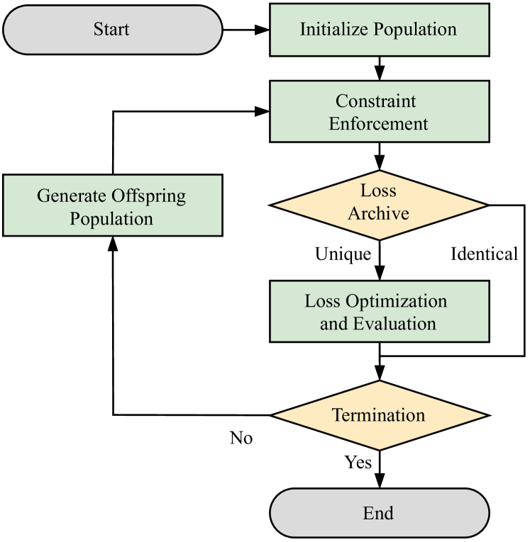
Figure 1. Overview of the EvoMAL algorithm.

The search algorithm used in the discrete outer optimization process of EvoMAL uses a prototypical implementation of GP. An overview of the algorithm is as follows:

• Initialization: To generate the initial population of candidate loss functions, 25 expression trees are randomly generated using Ramped Half-and-Half where the inner nodes are selected from the function set and the leaf nodes from the terminal set.

Subsequently, the main loop begins by performing the inner loss function optimization and evaluation process to determine each loss function’s respective fitness (discussed in detail in Section 3.2). Following this, a new offspring population of equivalent size is constructed via the crossover, mutation, selection, and elitism genetic operators.

• Crossover: For the crossover genetic operator, two loss functions are selected and then combined via a One-Point Crossover with a probability of 70%, which slices the two selected loss functions together to form a new loss function.

• Mutation: For the mutation genetic operator, a loss function is selected from the population, and a Uniform Mutation is applied with a mutation rate of 25%, which in place modifies a sub-expression at random with a newly generated sub-expression.

• Selection: Selection of candidate loss functions from the population for crossover and mutation is achieved via a standard Tournament Selection, which selects 4 loss functions from the population at random and returns the loss function with the best fitness score.

• Elitism: To ensure that performance does not degrade throughout the evolutionary process, elitism is used to retain the top-performing loss functions with an elitism rate of 5%.

The main loop is iteratively repeated up to 50 times until convergence, and the loss function with the best fitness is selected as the final learned loss function. For clarity, we include an overview of the outer optimization process in Figure 1.

Constraint Enforcement

When using GP, the learned expressions can occasionally violate two important constraints of a loss function. (1) Required Arguments Constraint: A loss function must have as arguments $f_{\theta}(x)$ and $y$ by definition. (2) Non-Negative Output Constraint: A loss function should always return a non-negative output such that $\forall x,\forall y,\forall f_{\theta}[\mathcal{M}(y,f_{\theta}(x))\geq 0]$. To resolve this we describe two corresponding correction strategies, which we summarize in Figure 2 for clarity.

1. Required Arguments Constraint: In (Gonzalez and Miikkulainen, 2020), violating expressions were assigned the worst-case fitness, such that selection pressure would phase out those loss functions from the population. Unfortunately, this approach degrades search performance, as a subset of the population is persistently searching infeasible regions of the search space. To resolve this, we propose a simple but effective corrections strategy to violating loss functions, which randomly selects a terminal node and replaces it with a random binary node, i.e. function node with an arity of 2, with arguments $f_{\theta}(x)$ and $y$ in no predetermined order (required for non-associative operations).

2. Non-Negative Output Constraint: An additional constraint optionally enforced in the EvoMAL algorithm is that the learned loss function should always return a non-negative output $\mathcal{M}:\mathbb{R}^{2}\rightarrow\mathbb{R}_{0}^{+}$. This is achieved via all learned loss function’s outputs being passed through an activation function $\varphi$, which was selected to be the smooth $Softplus(x)=ln(1+e^{x})$ activation.

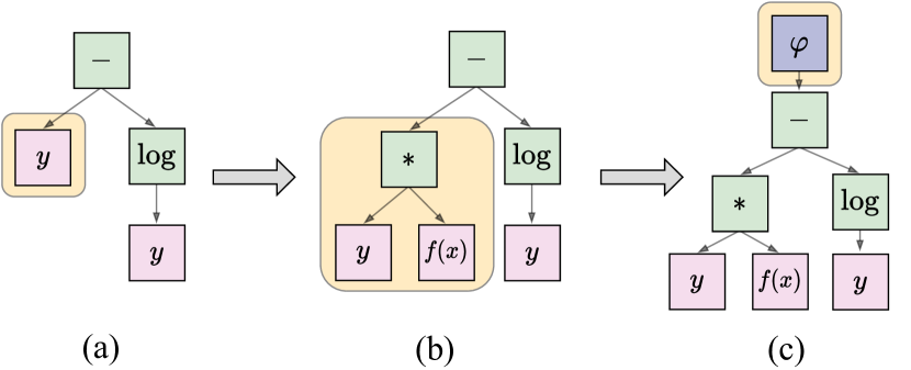
Figure 2. Overview of the constraint enforcement procedure, where (a) is a constraint violating expression, (b) demonstrates enforcing the required arguments constraint, and (c) shows enforcing the non-negative output constraint.

Loss Archival Strategy

As computational efficiency is often of concern when using population-based methods, a loss archival strategy based on a key-value pair structure with $\Theta(1)$ lookup is used to ensure that symbolically equivalent loss functions are not reevaluated.

3.2. Loss Function Optimization and Evaluation

(a) Example learned loss function $\mathcal{M}$.

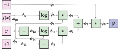
(b) Example meta-loss network $\mathcal{M}_{\phi}^{\mathsf{T}}$.

Figure 3. Overview of the transitional procedure used to covert $\mathcal{M}$ into a trainable meta-loss network $\mathcal{M}_{\phi}^{\mathsf{T}}$.

Numerous empirical results have shown that local search is imperative when using GP to get state-of-the-art results (Chen et al., 2015; Gonzalez and Miikkulainen, 2020). Therefore, unrolled differentiation, an efficient gradient-based local search approach is integrated into the proposed method. To integrate ML³ into the EvoMAL framework, we must first transform the expression tree-based representation of $\mathcal{M}$ into a compatible network-style representation. To achieve this, we propose the use of a transitional procedure that takes each loss function $\mathcal{M}$, represented as a GP expression and converts it into a trainable network, i.e. a weighted directed acyclic graph, as shown in Figure 3. First, a graph transpose operation $\mathcal{M}^{\mathsf{T}}$ is applied to reverse the edges such that they now go from the terminal (leaf) nodes to the root node. Following this, the edges of $\mathcal{M}^{\mathsf{T}}$ are parameterized by $\phi$, giving $\mathcal{M}_{\phi}^{\mathsf{T}}$, which we further refer to as a meta-loss network to delineate it clearly from its prior state.

Finally, to initialize $\mathcal{M}_{\phi}^{\mathsf{T}}$, the weights are sampled from $\phi\sim\mathcal{N}(1,1\mathrm{e}{-3})$, such that $\mathcal{M}_{\phi}^{\mathsf{T}}$ is initialized from its (near) original unit form, where the small amount of variance is to break network symmetry. For computational efficiency we use an adjacency list representation at implementation level which enables both the transpose and parameterization steps to occur simultaneously with a linear time and space complexity $\Theta(|\mathcal{V}|+|\mathcal{E}|)$ with respect to the number of vertices $\mathcal{V}$ and edges $\mathcal{E}$ (i.e. nodes and weights) in the learned loss function.

Extension to the Multi-Output Setting

To extend this framework to $\mathcal{C}$-way multi-output tasks (such as multi-class classification) we apply the binary version of the loss to each label and then take the sum across the outputs.

(2) $$\mathcal{M}_{\phi}^{\mathsf{T}}(y,f_{\theta}(x))=\sum_{i=1}^{\mathcal{C}}\mathcal{M}_{\phi,(i)}^{\mathsf{T}}(y_{(i)},f_{\theta,(i)}(x))$$

Loss Function Optimization

In: $\mathcal{M}_{\phi}^{\mathsf{T}}\leftarrow$ Loss function learned by GP
$\mathcal{S}_{meta}\leftarrow$ Number of meta gradient steps
$\mathcal{S}_{base}\leftarrow$ Number of base gradient steps

for $i\in\{0,...,S_{meta}\}$ do

1       for $j\in\{0,...,|\mathcal{D}_{Train}|\}$ do

2             $\theta\leftarrow$ Initialize parameters of base learner

3             for $k\in\{0,...,\mathcal{S}_{base}\}$ do

4                   $X_{j}$, $y_{j}$ $\leftarrow$ Sample task $\mathcal{T}_{j}\sim p(\mathcal{T})$

5                   $\mathcal{M}_{learned}\leftarrow\mathcal{M}_{\phi}^{\mathsf{T}}(y_{j},f_{\theta_{j}}(X_{j}))$

6                   $\theta_{new_{j}}\leftarrow\theta_{j}-\alpha\nabla_{\theta_{j}}\mathcal{M}_{learned}$

7                  

8            $\mathcal{L}_{task_{j}}\leftarrow\mathcal{L}_{\mathcal{T}}(y_{j},f_{\theta_{new_{j}}}(X_{j}))$

9            

10      $\phi\leftarrow\phi-\eta\nabla_{\phi}\sum_{j}\mathcal{L}_{task_{j}}$

11      

Algorithm 1 Inner Loss Function Optimization

For simplicity, we constrain the description of loss function optimization to the vanilla backpropagation case where the meta-training set $\mathcal{D}_{Train}$ contains one task, i.e. $|\mathcal{D}_{Train}|=1$; however, the full process where $|\mathcal{D}_{Train}|>1$ is summarized in Algorithm 1. To learn the weights $\phi$ of the meta-loss network $\mathcal{M}_{\phi}^{\mathsf{T}}$ at meta-training time with respect to base learner $f_{\theta}(x)$, we first use the initial values of $\phi$ to produce a loss value $\mathcal{M}_{learned}$ based on the forward propagation of $f_{\theta}(x)$.

(3) $$\mathcal{M}_{learned}=\mathcal{M}_{\phi}^{\mathsf{T}}(y,f_{\theta}(x))$$

Using $\mathcal{M}_{learned}$, the weights $\theta$ are optimized by taking the gradient of the loss value with respect to $\theta$, where $\alpha$ is the base learning rate as shown in Equation (4). Note, multiple gradient steps of $\theta$ can be taken here, which requires back-propagating through a chain of $f_{\theta}(x)$ gradient steps; however, in practice we find similar to (Bechtle et al., 2021), that a single gradient step on $\theta$ is sufficient.

(4) $$\begin{split}\theta_{new}&=\theta-\alpha\nabla_{\theta}\mathcal{M}_{\phi}^{\mathsf{T}}(y,f_{\theta}(x))\\ &=\theta-\alpha\nabla_{\theta}\mathbb{E}_{{X},y}\big{[}\mathcal{M}_{learned}\big{]}\end{split}$$

This gradient computation can be decomposed via the chain rule into the gradient of $\mathcal{M}_{\phi}^{\mathsf{T}}$ with respect to the product of the base models predictions $f_{\theta}(x)$ and the gradient of $f$ with parameters $\theta$.

(5) $$\theta_{new}=\theta-\alpha\nabla_{f}\mathcal{M}_{\phi}^{\mathsf{T}}(y,f_{\theta}(x))\nabla_{\theta}f_{\theta}(x)$$

Following this, $\theta$ has been updated to $\theta_{new}$ based on the current meta-loss network weights; $\phi$ now needs to be updated to $\phi_{new}$ based on how much learning progress has been made. Using the new base learner weights $\theta_{new}$ as a function of $\phi$, we utilize the concept of a task loss $\mathcal{L}_{\mathcal{T}}$ (inner objective) to produce a loss value $\mathcal{L}_{task}$ to optimize $\phi$ through $\theta_{new}$.

(6) $$\mathcal{L}_{task}=\mathcal{L}_{\mathcal{T}}(y,f_{\theta_{new}}(x))$$

where $\mathcal{L}_{\mathcal{T}}$ is selected based on the respective application — for example, the mean squared error ($MSE$) loss for the task of regression, binary cross-entropy ($BCE$) loss for binary classification, and categorical cross-entropy ($CCE$) loss for multi-class classification. Optimization of the meta-loss network loss weights $\phi$ now occurs by taking the gradient of $\mathcal{L}_{\mathcal{T}}$ with respect to $\phi$, where $\eta$ is the meta learning rate.

(7) $$\begin{split}\phi_{new}&=\phi-\eta\nabla_{\phi}\mathcal{L}_{\mathcal{T}}(y,f_{\theta_{new}}(x))\\ &=\phi-\eta\nabla_{\phi}\mathbb{E}_{{X},y}\big{[}\mathcal{L}_{task}\big{]}\end{split}$$

where the gradient computation can be decomposed by applying the chain rule as shown in Equation (8) where the gradient with respect to the meta-loss network weights $\phi$ requires the new model parameters $\theta_{new}$.

(8) $$\phi_{new}=\phi-\eta\nabla_{f}\mathcal{L}_{\mathcal{T}}\nabla_{\theta_{new}}f_{\theta_{new}}\nabla_{\phi}\theta_{new}$$

This process is repeated for a predetermined number of meta gradient steps $S_{meta}$. Following each meta gradient step, the base learner weights $\theta$ is reset. Note that in Equations (4)–(5) and (7)–(8), the gradient computation can alternatively be performed via automatic differentiation. Figure 4 shows an example of one step of the inner loss optimization process used in EvoMAL to learn the meta-loss network weights $\phi$.

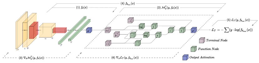
Figure 4. Example of one step of the inner loss optimization process used in EvoMAL to learn the weights $\phi$ of the meta-loss network $\mathcal{M}_{\phi}^{\mathsf{T}}$ with respect to the base network $f_{\theta}(x)$ shown (left) as the popular LeNet-5 architecture at meta-training time.

Loss Function Evaluation

In: $\mathcal{M}_{\phi}^{\mathsf{T}}\leftarrow$ Loss function learned by EvoMAL
$S_{base}\leftarrow$ Number of base gradient steps

1

for $i\in\{0,...,|\mathcal{D}_{Train}|\}$ do

2       $\theta_{i}\leftarrow$ Initialize parameters of base learner $f_{\theta_{i}}$

3       $X_{i}$, $y_{i}$ $\leftarrow$ Sample task $\mathcal{T}_{i}\sim p(\mathcal{T})$

4       for $j\in\{0,...,S_{base}\}$ do

5             $\mathcal{M}_{learned}\leftarrow\mathcal{M}_{\phi}^{\mathsf{T}}(y_{i},f_{\theta_{i}}(X_{i}))$

6             $\theta_{i}\leftarrow\theta_{i}-\alpha\nabla_{\theta_{i}}\mathcal{M}_{learned}$

7            

$\mathcal{F}\leftarrow\frac{1}{|\mathcal{D}_{Train}|}\sum_{i}\mathcal{L}_{\mathcal{P}}(y_{i},f_{\theta_{i}}(X_{i}))$

Algorithm 2 Loss Function Evaluation

To derive the fitness $\mathcal{F}$ of $\mathcal{M}_{\phi}^{\mathsf{T}}$, a conventional training procedure is used as summarized in Algorithm 2, where $\mathcal{M}_{\phi}^{\mathsf{T}}$ is used in place of a traditional loss function to train $f_{\theta}(x)$ over a predetermined number of base gradient steps $S_{base}$. This training process is identical to training at meta-testing time. The final average inference performance of $\mathcal{M}_{\phi}^{\mathsf{T}}$ across all the tasks in $\mathcal{D}_{Train}$ is assigned to $\mathcal{F}$, where any differentiable or non-differentiable performance metric $\mathcal{L}_{\mathcal{P}}$ (outer objective) can be used. In our experiments, we assign $\mathcal{L}_{\mathcal{P}}$ to be the $\small MSE\normalsize$ for regression, and error rate ($\small ER\normalsize$) for classification.

(9) $$\mathcal{F}=\frac{1}{|\mathcal{D}_{Train}|}\sum_{i}\mathcal{L}_{\mathcal{P}}(y_{i},f_{\theta_{i}}(X_{i}))$$

4. Experimental Design

In this section, we evaluate the performance of EvoMAL for the task of loss function learning. A set of experiments are conducted across four datasets and the performance is contrasted against a representative set of methods implemented in DEAP (Fortin et al., 2012), PyTorch (Paszke et al., 2019) and Higher (Grefenstette et al., 2019), which are as follows:

• Baseline – Directly using $\mathcal{L}_{\mathcal{T}}$ as the loss function, i.e. using loss functions $\small MSE\normalsize$, $\small BCE\normalsize$ or $\small CCE\normalsize$ respectively.

• Random – Pure random search on the symbolic search space proposed in Section 3.1, where loss functions represented as expression trees are randomly generated with an equivalent number of evaluations to EvoMAL.

• GP-LFL – A proxy method used to aggregate previous GP-based approaches for loss function learning without any local search mechanisms, using an identical setup to EvoMAL excluding Section 3.1.

• ML³ Supervised – Gradient-based loss learning method proposed in (Bechtle et al., 2021), which uses a parametric loss function defined by a two hidden layer feed-forward network trained with the method shown in Section 3.2.

The experimental design intends to isolate and highlight the effects of the different components in EvoMAL, to validate the effectiveness of hybridizing existing loss function learning approaches into one unified framework. The code for reproducing all the experiments can be found at: https://github.com/Decadz/Evolved-Model-Agnostic-Loss.

4.1. Benchmark Problems

For all benchmark problems, stochastic gradient descent ($\small SGD\normalsize$) is used as the optimizer similar to (Gonzalez and Miikkulainen, 2020; Bechtle et al., 2021; Andrychowicz et al., 2016), with a fixed base-learning rate $\alpha$ and meta-learning rate $\eta$ equal to $1\mathrm{e}{-3}$. All base networks are initialized via Xavier Glorot uniform initialization (Glorot and Bengio, 2010).

• Sine: A tabulated regression problem originally proposed in (Finn, 2018), which involves regressing sine waves, where the amplitude and phase of the sinusoids are varied between tasks. The amplitude varies within $[0.2,5.0]$ and the phase varies within $[-\pi,\pi]$. During meta-training time, five sine waves are generated where points are sampled uniformly from $[-2.0,2.0]$, and at meta-testing time five sine waves are also generated but are uniformly sampled from $[-5.0,5.0]$. Identical to (Bechtle et al., 2021), the base network is a simple feed-forward neural network with 2 dense layers with ReLU activation function, using 40 hidden units each. Training occurs over $S_{meta}=500$ and $S_{base}=100$ gradient steps with a fixed batch size of $100$.

• MNIST: An image classification problem originally presented in (LeCun et al., 1998) that involves classifying images of hand-drawn numeric digits. Identical to (Bechtle et al., 2021), we partition the original dataset into five separate binary classification tasks (to simulate a prototypical meta-learning setup) where $\mathcal{D}_{Train}$ contains 1 task and $\mathcal{D}_{Test}$ contains 4. The base network is chosen to be the well-known LeNet-5 convolutional neural network architecture, which is trained over $S_{meta}=1,000$ and $S_{base}=250$ gradient steps respectively with a batch size of $128$.

• CIFAR-10: An image classification problem taken from (Krizhevsky and Hinton, 2009), containing images from 10 different classes. Analogous to the previous dataset, we partition the problem into two separate multi-class classification tasks for meta-training and meta-testing, respectively, where $\mathcal{D}_{Train}$ and $\mathcal{D}_{Test}$ contain 5 distinct classes each. The base network is a convolutional neural network with the following architecture: 5x5 convolution with 32 filters, max pooling, batch normalization, 5x5 convolution with 64 filters, max pooling, batch normalization, dense layer with 256 nodes, dense layer with 128 nodes. Training occurs over $S_{meta}=1,000$ and $S_{base}=2,000$ gradient steps with a batch size of $256$.

• Surname: A character-level text recognition problem taken from (Rao and McMahan, 2019), where the objective is to classify the nationality of surnames from 18 classes. We partition the problem into two separate multi-class classification tasks, where $\mathcal{D}_{Train}$ and $\mathcal{D}_{Test}$ contain 9 distinct classes each. The base network is a recurrent neural network with the following architecture: an embedding layer with an output dimension of 256, an LSTM layer with 64 units, and a dense layer with 256 nodes. Training occurs over $S_{meta}=1,000$ and $S_{base}=2,000$ gradient steps with a batch size of $256$.

5. Results and Analysis

Table 2. Results reporting the mean $\pm$ standard deviation final inference performance across 10 independent executions of each algorithm, where the MSE is reported for Sine, and the ER for MNIST, CIFAR-10 and Surname.

		Sine	MNIST	CIFAR-10	Surname
(a) Training Tasks	Baseline	3.0280$\pm$1.0911	0.0414$\pm$0.0029	0.0654$\pm$0.0079	0.4224$\pm$0.0930
	Random	1.4115$\pm$0.7688	0.0560$\pm$0.0232	0.0642$\pm$0.0301	0.3197$\pm$0.0315
	GP-LFL	1.2844$\pm$0.8155	0.0387$\pm$0.0278	0.0619$\pm$0.1013	0.2005$\pm$0.0944
	ML3 Supervised	2.1073$\pm$0.7500	0.0215$\pm$0.0054	0.0323$\pm$0.0099	0.2410$\pm$0.0237
	EvoMAL	1.2670$\pm$0.8052	0.0056$\pm$0.0009	0.0019$\pm$0.0021	0.1405$\pm$0.0162

(a)

		Sine	MNIST	CIFAR-10	Surname
(b) Testing Tasks	Baseline	4.0735$\pm$1.5581	0.0258$\pm$0.0132	0.0340$\pm$0.0137	0.2025$\pm$0.0231
	Random	3.8963$\pm$2.3903	0.0592$\pm$0.0516	0.0352$\pm$0.0231	0.1970$\pm$0.0611
	GP-LFL	3.3212$\pm$1.4041	0.0265$\pm$0.0286	0.0407$\pm$0.0741	0.1714$\pm$0.1168
	ML3 Supervised	3.5872$\pm$1.8257	0.0153$\pm$0.0080	0.0149$\pm$0.0041	0.1608$\pm$0.0283
	EvoMAL	3.3099$\pm$1.3685	0.0053$\pm$0.0028	0.0006$\pm$0.0008	0.0921$\pm$0.0119

(b)

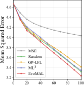
(a) Sine

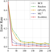
(b) MNIST

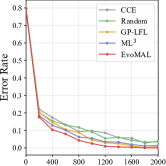
(c) CIFAR-10

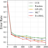
(d) Surname

Figure 5. Mean meta-testing learning curves on the out-of-sample testing tasks across 10 independent executions of each algorithm, showing the performance (y-axis) against gradient steps (x-axis). Best viewed in color.

We present the final inference performance at meta-testing time using the different benchmark methods in Table 2b, where (a) presents the in-sample performance on the meta-training tasks and (b) presents the out-of-sample performance on the meta-testing tasks. Analyzing the quantitative results, it is shown that EvoMAL consistently achieves significantly better final inference performance on each of the tested datasets, with much lower $\small MSE\normalsize$s on Sine, and notably lower $\small ER\normalsize$s on MNIST, CIFAR-10, and Surname. The strong in-sample performance demonstrates the effectiveness of EvoMAL in the single-task learning regime, while the out-of-sample performance successfully illustrates the high generalization capabilities when extended to new unseen tasks at meta-testing time.

5.1. Comparisons with Benchmark Methods

In most cases, a clear improvement is observed by using loss function learning techniques, strongly motivating the use of learned loss functions in favor of handcrafted loss functions. Concerning random search, improved performance is achieved on Sine and Surname, similar performance on CIFAR-10 and worse on MNIST compared to the baseline. These results suggest that with the dense symbolic search space containing many promising loss functions, improved search mechanisms are required to achieve better results. The later results by GP-LFL and ML³ empirically confirms this and shows that there is a sufficient exploitable structure in this optimization problem to motivate the design of more sophisticated loss function learning techniques.

Contrasting the performance of EvoMAL to its derivative methods GP-LFL and ML³, notable gains in inference performance are shown on all the tested datasets. These results reveal two key findings: first, further evidence that GP-based methods benefit significantly from introducing local search mechanisms, and second that gradient-based methods can successfully be utilized to achieve this task in a computationally tractable way. Our experiments were all conducted on a single consumer-level GPU, in contrast to (Gonzalez and Miikkulainen, 2020), which required a supercomputer and significantly reduced values of $S_{base}$ at meta-training time.

5.2. Convergence and Sample-Efficiency

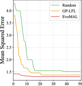
(a) Sine

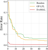
(b) MNIST

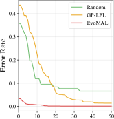
(c) CIFAR-10

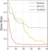
(d) Surname

Figure 6. Mean meta-training learning curves across 10 independent executions of each algorithm, showing the fitness score (y-axis) against outer iterations (x-axis), where an iteration is equivalent to 25 evaluations. Best viewed in color.

To further discern the benefits of using the learned loss functions produced by EvoMAL, the meta-testing learning curves on the in-sample and out-of-sample tasks are presented in Figure 5. Examining the qualitative results, it is observed that EvoMAL consistently produces improved performance compared to the benchmark methods, and it does so in far fewer gradient steps at all stages in the learning process, demonstrating improved sample efficiency and convergence capabilities, which is a desirable characteristic in regimes where either data or computational resources are low. Furthermore, the performance generally shows that EvoMAL only requires a small subset of the total gradient steps to surpass the final performance of the baseline.

5.3. Meta-Training Dynamics

To analyze the search effectiveness of EvoMAL the meta-training learning curves comparing the search performance (as quantified by the fitness function) at each iteration are given in Figure 6. Based on the results, it is evident that adding local search mechanisms into the EvoMAL framework dramatically reduces the total number of iterations needed to find performant loss functions compared to random search and GP-LFL. Furthermore, while EvoMAL often finds comparable fitness loss functions to GP-LFL after 50 iterations, the performance when evaluated, i.e. at meta-testing time, corresponds to a better generalizing loss function compared to GP-LFL as shown in Table 2b.

5.4. Loss Function Paramaterization

Table 3. Contrasting the mean $\pm$ standard deviation number of trainable loss parameters $\phi$ between ML³ and EvoMAL.

	Sine	MNIST	CIFAR-10	Surname
ML3	2,650	2,650	2,650	2,650
EvoMAL	30.9 $\pm$ 10.3	30.8 $\pm$ 6.8	26.8 $\pm$ 9.5	28.3 $\pm$ 13

In addition to the performance benefits of EvoMAL, a compelling finding is that compared to its gradient-based derivative method, ML³, only a small fraction of the number of trainable loss parameters $\phi$ is required, as shown in Table 3, where the meta-loss networks in ML³ use a feed-forward neural network with two input nodes followed by two dense layers of 50 nodes each and one output node (Bechtle et al., 2021). These results show that in ML³, the meta-loss networks are significantly over-parameterized, as less than $\sim$1-2% of the total number of trainable loss parameters $\phi$ are needed in the loss functions learned by EvoMAL compared to that of ML³ across all the tested datasets. Consequently, the loss functions learned by EvoMAL have improved inference speed, i.e. reduced cost to compute loss values at meta-testing time, due to not having to propagate through so many parameters.

6. Conclusions and Future Work

This work presents a new framework for meta-learning symbolic loss function via a hybrid neuro-symbolic search approach called Evolved Model-Agnostic Loss (EvoMAL). The proposed method poses the problem of loss function learning in terms of a bilevel optimization problem, where the outer optimization problem involved learning a set of symbolic loss functions via GP, and the inner optimization problem consisted of learning the weights of the parameterized loss functions found in the outer optimization process via unrolled differentiation. Integration of the outer and inner optimization problems was performed seamlessly by introducing a linear time transition procedure converting the GP expression tree-based loss functions into trainable meta-loss networks.

Our analysis of the learned loss functions produced by the newly proposed framework shows several benefits compared to handcrafted loss functions, and state-of-the-art loss function learning techniques. Empirical results show improved inference performance, convergence, and sample efficiency. Furthermore, this performance can successfully generalize to new unseen tasks not seen at meta-training time. Unlike existing methods for loss function learning, the proposed framework can be combined with any model representation amenable to a gradient-descent style training procedure for any supervised learning task, due to the generality in the search space design. Additionally, EvoMAL is the first GP-based loss function learning approach to integrate local search mechanisms into the learning process in a computationally feasible manner.

Despite the effectiveness of EvoMAL, there are still aspects of the framework that can be further improved upon and developed in future work. Firstly, we posit that introducing rejection protocols that filter out non-promising or gradient-equivalent loss functions similar to what was proposed in (Liu et al., 2021) and (Li et al., 2021), can reduce the number of evaluations required, thus reducing the runtime further. In addition, investigating alternative meta-optimization strategies such as implicit differentiation (Lorraine et al., 2020) or first-order gradient-based alternatives (Nichol et al., 2018) to unrolled differentiation is a promising area to explore, since a computational bottleneck in EvoMAL, and its derivative method ML³ is having to differentiate through the optimization path.

References

- (1)
- Altae-Tran et al. (2017) Han Altae-Tran, Bharath Ramsundar, Aneesh S Pappu, and Vijay Pande. 2017. Low Data Drug Discovery with One-Shot Learning. ACS central science 3, 4 (2017), 283–293.
- Andrychowicz et al. (2016) Marcin Andrychowicz, Misha Denil, Sergio Gomez, Matthew W Hoffman, David Pfau, Tom Schaul, Brendan Shillingford, and Nando De Freitas. 2016. Learning to learn by gradient descent by gradient descent. In Advances in neural information processing systems. 3981–3989.
- Balaji et al. (2018) Yogesh Balaji, Swami Sankaranarayanan, and Rama Chellappa. 2018. MetaReg: Towards Domain Generalization using Meta-Regularization. Advances in Neural Information Processing Systems 31 (2018), 998–1008.
- Bechtle et al. (2021) Sarah Bechtle, Artem Molchanov, Yevgen Chebotar, Edward Grefenstette, Ludovic Righetti, Gaurav Sukhatme, and Franziska Meier. 2021. Meta-Learning via Learned Loss. In 2020 25th International Conference on Pattern Recognition (ICPR). IEEE, 4161–4168.
- Bengio et al. (1994) Samy Bengio, Yoshua Bengio, and Jocelyn Cloutier. 1994. Use of Genetic Programming for the Search of a New Learning Rule for Neural Networks. In Proceedings of the First IEEE Conference on Evolutionary Computation. IEEE World Congress on Computational Intelligence. IEEE, 324–327.
- Chen et al. (2022) Can Chen, Xi Chen, Chen Ma, Zixuan Liu, and Xue Liu. 2022. Gradient-based bi-level optimization for deep learning: A survey. arXiv preprint arXiv:2207.11719 (2022).
- Chen et al. (2015) Qi Chen, Bing Xue, and Mengjie Zhang. 2015. Generalisation and Domain Adaptation in GP with Gradient Descent for Symbolic Regression. In 2015 IEEE congress on evolutionary computation (CEC). IEEE, 1137–1144.
- Co-Reyes et al. (2021) John D Co-Reyes, Yingjie Miao, Daiyi Peng, Esteban Real, Sergey Levine, Quoc V Le, Honglak Lee, and Aleksandra Faust. 2021. Evolving Reinforcement Learning Algorithms. arXiv preprint arXiv:2101.03958 (2021).
- Collet et al. (2022) Alan Collet, Antonio Bazco-Nogueras, Albert Banchs, and Marco Fiore. 2022. Loss meta-learning for forecasting. https://openreview.net/forum?id=rczz7TUKIIB
- Deledalle et al. (2014) Charles-Alban Deledalle, Samuel Vaiter, Jalal Fadili, and Gabriel Peyré. 2014. Stein Unbiased GrAdient estimator of the Risk (SUGAR) for multiple parameter selection. SIAM Journal on Imaging Sciences 7, 4 (2014), 2448–2487.
- Ding et al. (2022) Yadong Ding, Yu Wu, Chengyue Huang, Siliang Tang, Yi Yang, Longhui Wei, Yueting Zhuang, and Qi Tian. 2022. Learning to learn by jointly optimizing neural architecture and weights. In Proceedings of the IEEE/CVF Conference on Computer Vision and Pattern Recognition. 129–138.
- Domke (2012) Justin Domke. 2012. Generic methods for optimization-based modeling. In Artificial Intelligence and Statistics. PMLR, 318–326.
- Elsken et al. (2020) Thomas Elsken, Benedikt Staffler, Jan Hendrik Metzen, and Frank Hutter. 2020. Meta-learning of neural architectures for few-shot learning. In Proceedings of the IEEE/CVF conference on computer vision and pattern recognition. 12365–12375.
- Finn (2018) Chelsea Finn. 2018. Learning to learn with gradients. Ph. D. Dissertation. UC Berkeley.
- Finn et al. (2017) Chelsea Finn, Pieter Abbeel, and Sergey Levine. 2017. Model-Agnostic Meta-Learning for Fast Adaptation of Deep Networks. In International Conference on Machine Learning. PMLR, 1126–1135.
- Fortin et al. (2012) Félix-Antoine Fortin, François-Michel De Rainville, Marc-André Gardner Gardner, Marc Parizeau, and Christian Gagné. 2012. DEAP: Evolutionary Algorithms Made Easy. The Journal of Machine Learning Research 13, 1 (2012), 2171–2175.
- Franceschi et al. (2017) Luca Franceschi, Michele Donini, Paolo Frasconi, and Massimiliano Pontil. 2017. Forward and reverse gradient-based hyperparameter optimization. In International Conference on Machine Learning. PMLR, 1165–1173.
- Franceschi et al. (2018) Luca Franceschi, Paolo Frasconi, Saverio Salzo, Riccardo Grazzi, and Massimiliano Pontil. 2018. Bilevel programming for hyperparameter optimization and meta-learning. In International Conference on Machine Learning. PMLR, 1568–1577.
- Gao et al. (2021) Boyan Gao, Henry Gouk, and Timothy M Hospedales. 2021. Searching for Robustness: Loss Learning for Noisy Classification Tasks. arXiv preprint arXiv:2103.00243 (2021).
- Gao et al. (2022) Boyan Gao, Henry Gouk, Yongxin Yang, and Timothy Hospedales. 2022. Loss function learning for domain generalization by implicit gradient. In International Conference on Machine Learning. PMLR, 7002–7016.
- Glorot and Bengio (2010) Xavier Glorot and Yoshua Bengio. 2010. Understanding the difficulty of training deep feedforward neural networks. In Proceedings of the thirteenth international conference on artificial intelligence and statistics. JMLR Workshop and Conference Proceedings, 249–256.
- Gonzalez and Miikkulainen (2020) Santiago Gonzalez and Risto Miikkulainen. 2020. Improved Training Speed, Accuracy, and Data Utilization Through Loss Function Optimization. In 2020 IEEE Congress on Evolutionary Computation (CEC). IEEE, 1–8.
- Gonzalez and Miikkulainen (2021) Santiago Gonzalez and Risto Miikkulainen. 2021. Optimizing Loss Functions through Multi-Variate Taylor Polynomial Parameterization. In Proceedings of the Genetic and Evolutionary Computation Conference. 305–313.
- Grabocka et al. (2019) Josif Grabocka, Randolf Scholz, and Lars Schmidt-Thieme. 2019. Learning Surrogate Losses. arXiv preprint arXiv:1905.10108 (2019).
- Grefenstette et al. (2019) Edward Grefenstette, Brandon Amos, Denis Yarats, Phu Mon Htut, Artem Molchanov, Franziska Meier, Douwe Kiela, Kyunghyun Cho, and Soumith Chintala. 2019. Generalized Inner Loop Meta-Learning. arXiv preprint arXiv:1910.01727 (2019).
- Hospedales et al. (2020) Timothy Hospedales, Antreas Antoniou, Paul Micaelli, and Amos Storkey. 2020. Meta-learning in neural networks: A survey. arXiv preprint arXiv:2004.05439 (2020).
- Houthooft et al. (2018) Rein Houthooft, Yuhua Chen, Phillip Isola, Bradly Stadie, Filip Wolski, OpenAI Jonathan Ho, and Pieter Abbeel. 2018. Evolved Policy Gradients. In Advances in Neural Information Processing Systems, Vol. 31. 5405–5414. https://proceedings.neurips.cc/paper/2018/file/7876acb66640bad41f1e1371ef30c180-Paper.pdf
- Huang et al. (2019) Chen Huang, Shuangfei Zhai, Walter Talbott, Miguel Bautista Martin, Shih-Yu Sun, Carlos Guestrin, and Josh Susskind. 2019. Addressing the Loss-Metric Mismatch with Adaptive Loss Alignment. In International Conference on Machine Learning. PMLR, 2891–2900.
- Ignatov et al. (2019) Andrey Ignatov, Radu Timofte, Andrei Kulik, Seungsoo Yang, Ke Wang, Felix Baum, Max Wu, Lirong Xu, and Luc Van Gool. 2019. AI Benchmark: All About Deep Learning on Smartphones in 2019. In 2019 IEEE/CVF International Conference on Computer Vision Workshop (ICCVW). IEEE, 3617–3635.
- Kim et al. (2018) Jaehong Kim, Sangyeul Lee, Sungwan Kim, Moonsu Cha, Jung Kwon Lee, Youngduck Choi, Yongseok Choi, Dong-Yeon Cho, and Jiwon Kim. 2018. Auto-meta: Automated gradient based meta learner search. arXiv preprint arXiv:1806.06927 (2018).
- Koza (1992) John R Koza. 1992. Genetic programming: on the programming of computers by means of natural selection. Vol. 1. MIT press.
- Krizhevsky and Hinton (2009) Alex Krizhevsky and Geoffrey Hinton. 2009. Learning Multiple Layers of Features from Tiny Images. (2009).
- LeCun et al. (1998) Yann LeCun, Léon Bottou, Yoshua Bengio, and Patrick Haffner. 1998. Gradient-Based Learning Applied to Document Recognition. Proc. IEEE 86, 11 (1998), 2278–2324.
- Li et al. (2021) Hao Li, Tianwen Fu, Jifeng Dai, Hongsheng Li, Gao Huang, and Xizhou Zhu. 2021. AutoLoss-Zero: Searching Loss Functions from Scratch for Generic Tasks. arXiv preprint arXiv:2103.14026 (2021).
- Li et al. (2019) Yiying Li, Yongxin Yang, Wei Zhou, and Timothy Hospedales. 2019. Feature-critic networks for heterogeneous domain generalization. In International Conference on Machine Learning. PMLR, 3915–3924.
- Liu et al. (2021) Peidong Liu, Gengwei Zhang, Bochao Wang, Hang Xu, Xiaodan Liang, Yong Jiang, and Zhenguo Li. 2021. Loss Function Discovery for Object Detection via Convergence-Simulation Driven Search. arXiv preprint arXiv:2102.04700 (2021).
- Lorraine et al. (2020) Jonathan Lorraine, Paul Vicol, and David Duvenaud. 2020. Optimizing millions of hyperparameters by implicit differentiation. In International Conference on Artificial Intelligence and Statistics. PMLR, 1540–1552.
- Maclaurin et al. (2015) Dougal Maclaurin, David Duvenaud, and Ryan Adams. 2015. Gradient-based hyperparameter optimization through reversible learning. In International conference on machine learning. PMLR, 2113–2122.
- Ni et al. (2012) Ji Ni, Russ H Drieberg, and Peter I Rockett. 2012. The Use of an Analytic Quotient Operator in Genetic Programming. IEEE Transactions on Evolutionary Computation 17, 1 (2012), 146–152.
- Nichol et al. (2018) Alex Nichol, Joshua Achiam, and John Schulman. 2018. On First-Order Meta-Learning Algorithms. arXiv preprint arXiv:1803.02999 (2018).
- Paszke et al. (2019) Adam Paszke, Sam Gross, Francisco Massa, Adam Lerer, James Bradbury, Gregory Chanan, Trevor Killeen, Zeming Lin, Natalia Gimelshein, Luca Antiga, et al. 2019. Pytorch: An Imperative Style, High-Performance Deep Learning Library. Advances in neural information processing systems 32 (2019), 8026–8037.
- Peng (2020) Huimin Peng. 2020. A Comprehensive Overview and Survey of Recent Advances in Meta-Learning. arXiv preprint arXiv:2004.11149 (2020).
- Rajeswaran et al. (2019) Aravind Rajeswaran, Chelsea Finn, Sham Kakade, and Sergey Levine. 2019. Meta-learning with implicit gradients. (2019).
- Ramachandran et al. (2017) Prajit Ramachandran, Barret Zoph, and Quoc V Le. 2017. Searching for Activation Functions. arXiv preprint arXiv:1710.05941 (2017).
- Rao and McMahan (2019) Delip Rao and Brian McMahan. 2019. Natural Language Processing with PyTorch: Build Intelligent Language Applications using Deep Learning. ” O’Reilly Media, Inc.”.
- Raymond et al. (2023) Christian Raymond, Qi Chen, Bing Xue, and Mengjie Zhang. 2023. Online Loss Function Learning. arXiv e-prints, Article arXiv:2301.13247 (Jan. 2023), arXiv:2301.13247 pages. https://doi.org/10.48550/arXiv.2301.13247 arXiv:2301.13247 [cs.LG]
- Real et al. (2020) Esteban Real, Chen Liang, David So, and Quoc Le. 2020. AutoML-Zero: Evolving Machine Learning Algorithms From Scratch. In International Conference on Machine Learning. PMLR, 8007–8019.
- Rumelhart et al. (1986) David E Rumelhart, Geoffrey E Hinton, and Ronald J Williams. 1986. Learning representations by back-propagating errors. nature 323, 6088 (1986), 533–536.
- Schmidhuber (1987) Jürgen Schmidhuber. 1987. Evolutionary Principles in Self-Referential Learning. Ph. D. Dissertation. Technische Universität München.
- Schmidhuber (1992) Jürgen Schmidhuber. 1992. Learning to Control Fast-Weight Memories: An Alternative to Dynamic Recurrent Networks. Neural Computation 4, 1 (1992), 131–139.
- Scieur et al. (2022) Damien Scieur, Quentin Bertrand, Gauthier Gidel, and Fabian Pedregosa. 2022. The Curse of Unrolling: Rate of Differentiating Through Optimization. arXiv preprint arXiv:2209.13271 (2022).
- Shaban et al. (2019) Amirreza Shaban, Ching-An Cheng, Nathan Hatch, and Byron Boots. 2019. Truncated back-propagation for bilevel optimization. In The 22nd International Conference on Artificial Intelligence and Statistics. PMLR, 1723–1732.
- Smart and Zhang (2004) Will Smart and Mengjie Zhang. 2004. Applying Online Gradient Descent Search to Genetic Programming for Object Recognition. In Proceedings of the second workshop on Australasian information security, Data Mining and Web Intelligence, and Software Internationalisation-Volume 32. 133–138.
- Stanley et al. (2019) Kenneth O Stanley, Jeff Clune, Joel Lehman, and Risto Miikkulainen. 2019. Designing neural networks through neuroevolution. Nature Machine Intelligence 1, 1 (2019), 24–35.
- Topchy and Punch (2001) Alexander Topchy and William F Punch. 2001. Faster Genetic Programming based on Local Gradient Search of Numeric Leaf Values. In Proceedings of the genetic and evolutionary computation conference (GECCO-2001), Vol. 155162. Morgan Kaufmann.
- Vanschoren (2018) Joaquin Vanschoren. 2018. Meta-learning: A survey. arXiv preprint arXiv:1810.03548 (2018).
- Vilalta and Drissi (2002) Ricardo Vilalta and Youssef Drissi. 2002. A perspective view and survey of meta-learning. Artificial intelligence review 18, 2 (2002), 77–95.
- Wang et al. (2022) Qi Wang, Yue Ma, Kun Zhao, and Yingjie Tian. 2022. A comprehensive survey of loss functions in machine learning. Annals of Data Science 9, 2 (2022), 187–212.
- Wengert (1964) Robert Edwin Wengert. 1964. A simple automatic derivative evaluation program. Commun. ACM 7, 8 (1964), 463–464.
- Zhang and Smart (2005) Mengjie Zhang and Will Smart. 2005. Learning Weights in Genetic Programs Using Gradient Descent for Object Recognition. In Workshops on Applications of Evolutionary Computation. Springer, 417–427.