Influencing Bandits:
Arm Selection for Preference Shaping

Abstract

We consider a non stationary multi-armed bandit in which the population preferences are positively and negatively reinforced by the observed rewards. The objective of the algorithm is to shape the population preferences to maximize the fraction of the population favouring a predetermined arm. For the case of binary opinions, two types of opinion dynamics are considered—decreasing elasticity (modeled as a Polya urn with increasing number of balls) and constant elasticity (using the voter model). For the first case, we describe an Explore-then-commit policy and a Thompson sampling policy and analyse the regret for each of these policies. We then show that these algorithms and their analyses carry over to the constant elasticity case. We also describe a Thompson sampling based algorithm for the case when more than two types of opinions are present. Finally, we discuss the case where presence of multiple recommendation systems gives rise to a trade-off between their popularity and opinion shaping objectives.

Keywords:Multi-armed Bandits, Opinion Shaping, Contextual Bandits, Non-stationary rewards

I Introduction

Stochastic multi-armed bandit (MAB) algorithms are used in many applications. A canonical application is in recommendation systems that suggest one or more items from a fixed set of items to users of the system. Example uses of these recommendation systems are for suggesting items on e-commerce websites and on streaming services, recommending friends and connections on social networks, and for placing results and ads in search engines. The classical stochastic MAB setting is as follows. Users arrive sequentially and are recommended one of $N$ arms. The system obtains a random reward based on the user preference for the recommended arm. The reward distribution of each arm is assumed independent of all other rewards and is unknown. The objective of the MAB algorithm is to learn the best arm while minimizing the loss in cumulative reward, compared to that from an ideal or a reference algorithm, over a finite time horizon. Among the many extensions to this classical problem, the one relevant to our work is that of contextual bandits where the algorithm also has side information about the user’s preferences.

A key assumption made in the design and analyses of classical MAB algorithms is that the reward distributions of the arms do not change with time. This also implies that the preferences of the user population are assumed to not be affected by the sequence of arms that are played. From ones own experiences, the latter is clearly not always true—user preferencess are affected by the recommendations. In fact, the objective of advertisements is to persuade users to adopt particular preferences. With this motivation, in this paper, we make the reasonable assumption that user preferences are not independent of the recommendations and are in fact influenced by them. Specifically, we assume that the preferences of the users at any time, and hence the reward distributions from the arms, depends on the history of recommendations upto that time and is a function of the arms that are played and rewards accrued.

MAB algorithms are usually designed to find the best arm, the one with the highest expected reward, by a judicious combination of exploration and exploitation. Our objective is a marked departure from this: the goal is to actively use the preference reinforcements to influence the population preferences. This objective is similar in spirit to the emerging literature on opinion control, e.g., [5, 6, 7]. However, to the best of our knowledge, such an objective has not been explored in an MAB setting.

In this paper, we will assume that the recommendation system uses a contextual MAB algorithm to serve a multitype population with each type having a unique preferred arm. We allow both positive and negative influences to be simultaneously present—influence is positive when the recommended arm is liked by the user and the influence is negative when the recommendation is not liked by the user. Furthermore, we consider two kinds of time-dependent behavior of influence dynamics: (1) decreasing intensity of influence where the population becomes increasingly rigid in its preferences, and (2) constant intensity of influence where the degree of influence remains constant throughout the period of interest. The first model is motivated by the empirical observation that advertising gives diminishing returns [8],[9] and the second model is inspired by the popular voter model (introduced in [10]) which has been widely studied in the literature on opinion dynamics. For both these models we will first consider a system that is serving a population of two types with type 1 being the preferred type, i.e., the objective of the algorithm is to maximize the population of type 1 users at the ed of the time horizon $T.$

The following are the key contributions in the paper.

• Optimal policy to maximize type 1 population when reward statistics are known. Interestingly, the optimal policy does not necessarily recommend the favoured arm. [Section IV]

• An explore-then-commit (ETC) policy to maximize type 1 population when the reward statistics are unknown. This has to battle the twin tradeoffs—usual exploration-exploitation tradeoff and the decreasing ability to shape the preferences when the population has become more rigid. This is also shown to have logarithmic regret in the known time-horizon setting. [Section V]

• A Thompson sampling based policy to maximize type 1 population when the reward statistics are unknown. We show that this policy gives us logarithmic regret even if the time-horizon is unknown. [Section V]

• For the case of the constant influence model, we show that the analyses and the algorithms we obtained for the decreasing influence model stay valid. [Section VI]

• Finally, we present two different extensions, First, we describe an $N$-arm MAB for an $N$-type population. For the objective of maximising the type 1 population, we obtain the optimal policy when the reward matrix is known. We then extend the Thompson sampling algorithm to this case. This is considered in Section VII-A.

  A second extension is a model for two recommendation systems with competing objectives for the two-arm, two-type case. Some preliminary results are presented Section VII-B.

In the next section we discuss the related literature and delineate our work. The model and some preliminaries are set up in Section III. We conclude the paper with a discussion on directions of future work. All the proofs are carried in the appendix.

II Related Work

The literature on MAB algorithms is vast and varied and excellent textbook treatments that describe the basic models and several key variations are available in, e.g., [11, 1, 2, 3]. Our interest in this paper is on contextual bandits where the MAB has side information about the user. An early analysis of MABs with side information is in [12] although the term was coined in [4]. In this paper we consider contextual bandits where the type of the user is known to the algorithm before the recommendation is made.

As we mentioned earlier, in the classical setting the reward distributions on the arms remain the same and the rewards are independently realized for each user. There is however, an emerging literature on MAB algorithms that do not assume that reward distributions are the same at all times. In [13] the expected reward from any arm can change at any point and any number of times; changes are independent of the algorithm and the reward sequence. In rotting and recharging bandits, the arms have memory of when they were last recommended and the reward distribution depends on the delay since the last use of the arm. In the rotting bandit model [14], the expected reward from playing an arm decreases with the gap since the last play. The recharging bandit model [15] is the opposite—expected reward increases with the gap. The models of [16, 17] have similar objectives but are developed in a Markovian restless bandits setting. A generalisation of rotting and recharging bandits is considered in [18] where the mean rewards from the arms vary according to a Markov chain. Positive reinforcement of the population preferences based on the rewards seen is modelled in [19]. Here the preference in a multi-type user population is positively reinforced by positive rewards. However, this is not a contextual bandit setting and negative reinforcements are not modelled here.

None of the preceding are contextual bandits, i.e., they do not have side information about the user. Non stationary contextual bandits are considered in [20] but the time dependent behaviour of the arms is independent of the sample path of the user types and the rewards. In all of the preceding, the objective is to maximize the cumulative reward (minimize regret) and not to influence the population.

Our objective is to not maximize the rewards obtained but shape the preferences. In this there are similarities with the objectives in [5, 6, 7]. In [5], the objective is to rapidly converge to a desired asymptotic consensus in a social network. In [6, 7], open loop, optimal control techniques are used to shape the opinions in a social network. We do not deal with a social network, rather with the population that interacts with a platform like a recommendation system. We believe that this is the first work that models positive and negative reinforcements due to the rewards and has the the explicit objective of shaping the preferences in the population.

In the model that we describe in this paper, the preferences of the user population will be tracked by a Polyà urn [21], widely used to model random reinforcements; see [22] for an excellent tutorial and survey. Much of this literature is on characterization of the asymptotic composition of the urn. Our interest in this paper is to influence the composition of the urn.

III Model and Preliminaries

A population of two types of users is served by a recommendation system $S$ which recommends one of two arms to each arriving user. The two types of users are distinguished by their preference for one arm over another. Time is discrete and takes values $t\in[1:T].$ At time $t$, a user of type $X_{t}$ arrives, the type is observed by $S$ and the user is shown arm $A_{t}.$ Since the type is observed by $S$ before the arm recommendation is made, this is a contextual bandit. For much of the paper we will assume $A_{t}\in\{1,2\}$ and $X_{t}\in\{1,2\},$ i.e., we will consider a two-arm system serving a two-type population.

The probability of the incoming user at time $t$ being of a specific type is proportional to the fraction of users of that type in the population at time $t$. The fraction of users of a specific type in the population evolves over time. Specifically, the fraction of users in the population of a specific type at a given time is a function of the recommendations made to incoming users up to that time and the users’ response to those recommendations. For ease of exposition, we track the fraction of type 1 and type 2 users in the population via a virtual urn containing colored balls (colors 1 and 2 corresponding to, respectively, population types 1 and 2); the fraction of type 1 users in the population equals the fraction of type 1 balls in the urn.

Reward Structure. Suppose $X_{t}=i$ and $A_{t}=j,$ i.e., user at time $t$ is of type $i$ and is recommended arm $j.$ The user gets a random Bernoulli reward $W_{t}\in\{0,1\}$ with mean $b_{ij}.$ Let $B:=[[b_{ij}]]$ be the reward means matrix. Without loss of generality, we assume that $b_{ii}$ is the maximum in row $i$ of $B,$ i.e., type $i$ users prefer arm $i$ over others.

Population Dynamics. Let $Z_{i}(t)$ be the number of type $i$ balls in the urn at time $t.$ The user arriving at time $t$ is of type $i$ with probability $z_{i}(t)=Z_{i}(t)/(\sum_{j}Z_{j}(t)).$ $W_{t}$ is the realization of the reward at time $t$ and it causes the urn to be updated reflecting the change in the population type effected by the arm shown and the reward obtained. We consider two ways in which the update occurs. $N_{0}=Z_{1}(0)+Z_{2}(0)$ is the total number of balls at $t=0.$

1. Decreasing Influence Dynamics (DID) model. In this model, the total number of balls increases by one in each time-slot and the colour of the ball is determined as follows. If the user arriving at time $t$ is shown arm $j,$ and the user likes this arm (i.e., the random Bernoulli reward obtained is one) then the number of balls of type $j,$ (i.e., the type that has preference for the arm shown) increases by one. If the user does not like the arm shown, then the number of balls of type ${-j},$ (i.e., the type that has lower preference for the arm shown) increases by one. Formally,

   $$Z_{A_{t}}(t+1) =Z_{A_{t}}(t)+W_{t},$$

   $$Z_{-A_{t}}(t+1) =Z_{-A_{t}}(t)+(1-W_{t}).$$ (1)

   Here $-A_{t}$ is the arm that was not recommended. The population dynamics of (1) implies that the maximum possible change in the value of $z_{i}(t)$ decreases with $t.$ Thus the population of users, and hence the preferences, becomes less plastic with time. Real life examples of this setting are applications like Yelp which recommend restaurants to customers. Customers review or rate restaurants once they visit them. The ratings influence the preferences of future customors. Furthermore, since the number of reviews for each restaurant increase over time, the maximum possible change to the average rating decreases with time.

2. Constant Influence Dynamics (CID) model . In this model, the total number of balls in the urn remains constant over time. The influence of the rewards over the population is modeled as follows. If a user of type $X_{t}$ arriving at $t$ yields reward 1 when shown arm $A_{t}={-X_{t}}$ or reward 0 when shown arm $A_{t}={X_{t}}$ then one ball of type $-X_{t}$ changes its colour. The balls do not change type in the other two cases. Formally, defining $\theta_{t}$ to be the event $\{A_{t}={-X_{t}}\},$ the urn evolution will be

   $$Z_{A_{t}}(t+1) =Z_{A_{t}}(t)+\left(\mathbbm{1}_{\theta_{t}}\oplus W_{t}\right),$$

   $$Z_{-A_{t}}(t+1) =Z_{-A_{t}}(t)-\left(\mathbbm{1}_{\theta_{t}}\oplus W_{t}\right).$$ (2)

   Here the maximum possible change in the value of $z_{i}(t)$ remains constant over time. This model is inspired by the voter model of [10] which is usually defined on a graph. Here the voters interact with the recommendation system, one at a time, rather than with each other. Real life examples of this setting include tracking polls that use a focus group of the same set of individuals that are polled periodically to track the evolution of their collective opinion over time.

Observe that in both the models, the rewards are stationary, i.e., $b_{ij}$ does not chage with time. However, the preferences for the arms in the population, $z(t),$ is changing with time. Thus this is a non stationary contextual multi-armed bandit.

Remark. It is easy to see that both the models are a special case of the following general Markov decision process model. Let $(Z(t),X_{t})$ be the state of the system with $X_{t}$ being a function of $Z(t).$ The evolution of $Z(t+1),$ and hence $X_{t+1},$ depends on the action $A_{t}$ and on the reward $W_{t}.$

Algorithmic Goal. The goal of the recommendation system $S$ is to follow a trajectory $z(t)$ for $0<t\leq T$ that achieves the maximum possible increase at at every time $t.$ We will show in Theorem 2 that this also corresponds to maximizing $z(T)$ as $T\to\infty.$

We now formally define a policy.

Definition 1 (Policy).

A policy $\pi$ is a time indexed sequence of the tuples $(p_{t},q_{t})$ where, for all $t\in[1:T],$

$$p_{t} =P(A_{t}=a_{1}|X_{t}=1,z_{1}(t))$$

$$q_{t} =P(A_{t}=a_{2}|X_{t}=2,z_{1}(t)).$$ (3)

From the definition, $p_{t}$ is the probability of showing arm 1 to a type 1 user and $q_{t}$ is the probability of showing arm 2 to a type 2 user. The sequence of tuples $\{p_{t},q_{t}\}_{t>0}$ uniquely identifies a policy for the two-armed influencing bandit problem. We now formalize our goal by defining the notion of an optimal policy.

Definition 2 (Optimal policy).

An optimal policy for time $t$ is the value of $(p_{t},q_{t})$ that maximizes the expected increase in type 1 population in time slot $t,$ given the population profile at time $t,$ i.e.,

$$(p^{*}_{t},q_{t}^{*})=\arg\max_{(p_{t},q_{t})}\mathsf{E}\!\left(\Delta Z_{1}(t)\ |\ z_{1}(t)\right)$$ (4)

where $\Delta Z_{1}(t)=Z_{1}(t+1)-Z_{1}(t)$.

Remark. Observe that this definition is of a locally optimal policy. However, in Theorem 2 of the next section we show that the optimal policy is independent of $z_{1}(t)$ and thus the locally optimal policy is also optimal in a broader sense that is made more explicit.

Next we define the metrics of regret and cumulative regret for preference shaping which will be used to compare the performance of different policies. Let $\Delta Z_{1}^{\pi}(t)$ (resp. $\Delta Z_{1}^{*}(t)$) be the change in the population of type 1 balls in the urn at time $t$ given that we follow the policy $\pi$ (resp. the optimal policy) at time $t.$

Definition 3 (One-step regret).

Regret in a time slot $t,$ for policy $\pi,$ denoted by $R_{t}^{\pi},$ is defined as

$$R_{t}^{\pi}=\mathsf{E}\!\left(\Delta Z_{1}^{*}(t)-\Delta Z_{1}^{\pi}(t)\ |\ Z_{1}^{*}(t)=Z_{1}^{\pi}(t)\right).$$ (5)

The definition of cumulative regret follows naturally.

Definition 4 (Cumulative regret).

Cumulative regret ($R_{[1:T]}^{\pi}$) of a policy $\pi$ is defined as

$$R_{[1:T]}^{\pi}=\sum_{t=1}^{T}R_{t}^{\pi}.$$

Observe that in the definition of one-step regret, the expectation is conditioned on the population profile $Z_{1}(t)$ for both the optimal policy and candidate policy $\pi$ being the same at time $t^{-},$ before the policy is applied. The cumulative regret is just the sum of these one-step deviations.

We argue that a meaningful comparison between two policies in a time slot can be done when both are operating on the same composition of population. Hence, when defining one-step (or instantaneous) regret, we specify the population composition on which the optimal policy is being played. Such a metric is a useful, and informative, to compare policies, because if policy $A$ is better than another policy $B$ in maximizing the expected increase in type 1 balls in the urn at all time instants conditioned on the same initial state, then it will also incur a lesser regret for all time instants.

Adapting the commonly used definition of regret for our setting would define the regret of a candidate policy as the difference between the maximum possible value of $z_{T}$ and the value of $z_{T}$ under a candidate policy. We make a precise comparison between this commonly used definition and our definition in (5) in Appendix -A.

IV Preference Shaping with Known Rewards Matrix

In this and in the next section we consider the DID model in which the influence of the actions of $S$ and the observed rewards decreases with time. We begin by assuming that $S$ knows the reward means matrix $B$ and wants to maximize the expected proportion of type 1 users in the population at time $T.$ This case is interesting in its own right because it is directly useful when $B$ is exogenously available, e.g., from previously collected data. It also provides insight into the behavior of the optimal influence process. Thus it is a preliminary result that informs the design of algorithms for the case when $B$ is unknown.

The following theorem describes the optimal policy.

Theorem 1.

The optimal policy at time $t$ is

$$(p_{t}^{*},q_{t}^{*})=(\mathbbm{1}_{\{b_{11}+b_{12}-1>0\}},\mathbbm{1}_{\{b_{21}+b_{22}-1<0\}})$$ (6)

where $\mathbbm{1}_{\{\cdot\}}$ is the indicator function.

The optimal policy would have $S$ recommending arm $1$ to a type 1 arrival for all $t$ if $b_{11}>1-b_{12}$ and recommending arm $2$ otherwise. Recall that arm $1$ is the preferred arm for type 1 arrivals. We can interpret this to mean that $S$ should always recommend arm $1$ to type 1 users if they like arm $1$ more than they dislike arm $2,$ and should recommend arm $2$ otherwise. This is a result of the negative reinforcement that can happen if arm $1$ is not liked sufficiently strongly or if arm $2$ is liked strongly. Thus, for optimal preference shaping, the system may recommend arms which have a lower preferrence for the user.

Clearly, the policy of (6) in Theorem 1 gives us zero cumulative regret. However, it is not immediately clear if this policy maximizes the proportion of type 1 users in the population at time $T.$ To show that this is indeed the case, we first analyze the time evolution of the expected proportion for policy $\pi$ and state the following lemma.

Lemma 1.

Let $d_{1}:=p(1-b_{11})+(1-p)b_{12}$ and $d_{2}:=q(1-b_{22})+(1-q)b_{21}.$ Further, let $z_{1}(0)$ be the proportion of type 1 users at $t=0.$ For a policy $\pi$ with $(p_{t},q_{t})=(p,q),$ the expected proportion of type 1 users at time $t$ is

$$z_{1}(t)=\frac{d_{2}}{d_{1}+d_{2}}+\left(z_{1}(0)-\frac{d_{2}}{d_{1}+d_{2}}\right)\left(1+\frac{t}{N_{0}}\right)^{-(d_{1}+d_{2})}$$ (7)

Lemma 1 tells us that the expected proportion of type 1 users monotonically approaches $d_{2}/(d_{1}+d_{2})$ as $t\to\infty$ and is independent of $z_{1}(0).$ Thus, this is the maximum proportion that can be achieved using a policy of the form $(p_{t}=p,q_{t}=q)$. It turns out that the policy from (6) of Lemma 1 does indeed maximize the proportion of type 1 users in the population.

Theorem 2.

The optimal policy of (6) of Lemma 1 maximizes the expected asymptotic proportion of type 1 users and the maximum proportion is $\left(\frac{d_{2}}{d_{1}+d_{2}}\right).$

Thus, if the matrix of mean rewards $B$ is known, we can obtain a zero regret policy that also provably maximizes the expected proportion for the goal of preference shaping.

The preceding results are aimed at optimizing metrics that are in expectation. We can say more; specifically, we can provide long and short term sample path guarantees via stochastic approximation theory. Furthermore, the derivation of the mean trajectories as in Lemma 1 through the formation of an o.d.e can also be justified using this theory. We do this below.

Sample path guarantees. Recall that the classic stochastic approximation equation for which we have long term convergence guarantees is the following equation, introduced by Robbins and Monro in [23]

$$x_{t+1}=x_{t}+a(t)(h(x_{t})+M_{t+1}).$$

Here $h$ is Lipschitz, $M_{t}$ is a zero-mean martingale difference sequence and $\{a(t)\}$ are coefficients which satisfy the two conditions (1) $\sum_{t}a(t)=\infty$ and (2) $\sum_{t}a^{2}(t)<\infty$. For such an iteration, it is guaranteed that all sample paths of $x_{t}$ will converge to the equilibrium point of the o.d.e. $\dot{x}(t)=h(x(t))$ (i.e. $h(x)=0$) almost surely as $t\to\infty.$ Further, the maximum deviation from the o.d.e. trajectory in a fixed length time window $[t,t+T]$ also goes to 0 almost surely as t goes to $\infty$. A weaker error bound for finite time and constant stepsize $a(t)=a$ is given in [24].

We now analyze the difference between the trajectory of the o.d.e. obtained in the proof of Lemma 1 and a sample path of the stochastic sequence evolving according to (1) using stochastic approximation theory. Towards this goal, we first rewrite (1) into the classical Robbins-Monro form. For a fixed policy, the stochastic sequence of the number of type 1 balls, $Z_{1}(t),$ evolves as

$$Z_{1}(t+1) =Z_{1}(t)+\Delta Z_{1}(t)$$

$$=Z_{1}(t)+\left(E[\Delta Z_{1}(t)|z_{1}(t)]\right.$$

$$\hskip 25.0pt\left.+(\Delta Z_{1}(t)-E[\Delta Z_{1}(t)|z_{1}(t)])\right),$$

where $E[\Delta Z_{1}(t)|z_{1}(t)]=z_{1}(t)(1-d_{1})+(1-z_{1}(t))d_{2}$ (which can be shown directly from the definition of the DID model). Since $E[\Delta Z_{1}(t)|z_{1}(t)]$ is Lipschitz in $Z_{1}(t)$ and $M_{t}=\Delta Z_{1}(t)-E[\Delta Z_{1}(t)|z_{1}(t)]$ is a zero mean martingale difference sequence, this equation is in a constant stepsize form of the Robbins-Monro iteration and has been used to obtain the o.d.e. in the proof of Lemma 1. To get long term convergence guarantees, we divide the above equation by $(N_{0}+t+1)$ on both sides to obtain the following.

$$z_{1}(t+1) =\frac{1}{N_{0}+t+1}\left(Z_{1}(t)+E[\Delta Z_{1}(t)|z_{1}(t)]+M_{t}\right)$$

$$=\frac{N_{0}+t}{N_{0}+t+1}z_{1}(t)+\frac{1}{N_{0}+t+1}(E[\Delta Z_{1}(t)|z_{1}(t)]+M_{t})$$

$$=z_{1}(t)+\frac{1}{N_{0}+t+1}(E[\Delta Z_{1}(t)|z_{1}(t)]-z_{1}(t)+M_{t})$$

$$=z_{1}(t)+\frac{1}{N_{0}+t+1}(d_{2}-(d_{1}+d_{2})z_{1}(t)+M_{t})$$

In the preceding we have used $Z_{1}(t+1)/(N_{0}+t+1)=z_{1}(t+1).$ This last equation is now in the standard Robbins-Monro form as in [23], since $\sum_{t}1/(N_{0}+t+1)=\infty$ and $\sum_{t}1/(N_{0}+t+1)^{2}<\infty.$ Therefore, all sample paths followed by $z_{1}(t)$ converge asymptotically almost surely to $z_{1}=d_{2}/(d_{1}+d_{2}).$

Figure 1 shows an example comparison between the trajectories from 1, 10, and 100 samples paths. The figure also plots the trajectory of the o.d.e. obtained in Lemma 1. Observe that although a single sample path can have substantial deviations, averages of even a small number begins to track the o.d.e. rather closely. This observation was seen in all of our many simulations.

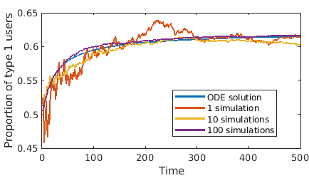
Figure 1: Trajectory of proportion of type 1 population. Comparison of o.d.e. solution and averages from 1, 10 amd 100 sample paths. We used $B$ with the values $b_{00}=0.9,$ $b_{01}=0.4,$ $b_{10}=0.2,$ and $b_{11}=0.6.$

V Preference Shaping with Unknown Rewards Matrix

When the rewards mean matrix $B$ is unknown, we face a two-fold trade-off in preference shaping. The first trade-off is the classical exploration-exploitation trade-off, where exploration involves correctly estimating the matrix $B$ and exploitation involves using the optimal policy derived in the previous section to maximise the fraction of type 1 population. The second trade-off is the decreasing plasticity (DID model) of the preferences modelled by the increasing number of balls in the urn. This puts additional pressure on exploitation of the estimated $B$ as soon as possible.

We consider two algorithms to address the two-fold trade-off. We first describe and analyze a naive explore-then-commit (ETC) algorithm. Next we describe a Thompson sampling (TS) based algorithm and also analyze it. We will see that if the time horizon $T$ is known, ETC can give logarithmic regret. The TS algorithm also gives logarithmic regret and has the advantage of not needing to know $T$ in the parametrization of the algorithm.

Our analyses of the algorithms will obtain upper bounds on the cumulative regret accrued by each algorithm. First we obtain the regret for a general policy $\pi=\{p_{t},q_{t}\}_{t>0}$ in the following lemma.

Lemma 2.

Define $\Delta_{1}:=|b_{11}+b_{12}-1|$ and $\Delta_{2}:=|b_{22}+b_{21}-1|$. The regret $R_{t}^{\pi}$ of a policy $\pi$ that has parameter values $(p_{t},q_{t})$ is given by

$$R_{t}^{\pi} =z_{1}(t)|\mathbbm{1}_{\{b_{11}+b_{12}-1>0\}}-p_{t}|\Delta_{1}$$

$$\hskip 36.135pt+(1-z_{1}(t))|\mathbbm{1}_{\{b_{21}+b_{22}-1<0\}}-q_{t}|\Delta_{2}.$$

V-A The Explore-Then-Commit (ETC) Algorithm

This algorithm has two phases. The exploration phase lasts for $m$ time units when each arm is recommended uniformly and the rewards mean matrix is estimated. This estimate is used to determine the optimal policy and commit to it during the remaining $(T-m)$ time units. Based on the preceding section and assuming that the estimates then use the optimal policy of the previous section (evaluated for the estimate $\hat{B}=[\hat{b}_{ij}]_{2\times 2}$) to maximize the proportion of type 1 users. Algorithm 1 describes the scheme in detail.

1Initialize $b_{ij}=0$, $n_{ij}=1$ for all $i,j\in\{1,2\}$;

2 for t = [1:m] do

3       $i\leftarrow$Type of user arrived;

4       Show arm $j$ chosen uniformly from $\{1,2\}$;

5       Collect reward $W_{t}$;

6       $b_{ij}+=W_{t}$;

7       $n_{ij}+=1$;

8      

9 end for

10$\hat{b}_{ij}\leftarrow b_{ij}/n_{ij}$ for all $i,j\in\{1,2\}$;

11 for t = [m+1:T] do

12       $i\leftarrow$Type of user arrived;

13       if i == 1 then

14             Show arm 1 w.p $\mathbbm{1}_{\{\hat{b}_{11}+\hat{b}_{12}-1>0\}}$  else show arm 2;

15      else

16             Show arm 2 w.p $\mathbbm{1}_{\{\hat{b}_{22}+\hat{b}_{21}-1<0\}}$ else show arm 1;

17       end if

18      

19 end for

20

Algorithm 1 The Explore-Then-Commit algorithm

We now use Lemma 2 to find the regret for this policy.

Lemma 3.

The cumulative regret, for the Explore-then-Commit policy with $m$ time units for exploring is

$$R_{[1:T]}^{\pi} =R_{explore}+R_{commit},$$

where

$$R_{explore} =0.5\left(\sum_{t=1}^{m}z_{1}(t)\right)\Delta_{1}+0.5\left(m-\sum_{t=1}^{m}z_{1}(t)\right)\Delta_{2}$$

$$R_{commit} =p_{err}\left(\sum_{t=m+1}^{T}z_{1}(t)\right)\Delta_{1}$$

$$\hskip 21.68121pt+q_{err}\left(T-m-\sum_{t=m+1}^{T}z_{1}(t)\right)\Delta_{2}$$

$$p_{err} =P((\hat{b}_{11}+\hat{b}_{12}-1)(b_{11}+b_{12}-1)<0)$$

$$q_{err} =P((\hat{b}_{22}+\hat{b}_{21}-1)(b_{22}+b_{21}-1)<0)$$

It now remains to derive bounds on the cumulative regret so that this policy can be compared to others. The general result has eluded us. However, we state the following result for the the special case of $b_{11}=b_{22}$ and $b_{12}=b_{21}.$

Theorem 3.

If $B$ is such that $b_{11}=b_{22}$ and $b_{12}=b_{21},$ the cumulative regret for the Explore-Then-Commit (ETC) policy is bounded above by

$$R_{[1:T]}^{ETC}\leq m\Delta_{1}/2+(T-m)\Delta_{1}e^{-m\Delta_{1}^{2}/8}$$ (8)

Further, using $m=8\log(T)/\Delta_{1}^{2}$ (to bound the regret in terms of $T$ and eliminate $m$), we get a logarithmic regret, i.e.,

$$R_{ETC}\leq\frac{4}{\Delta_{1}}\log(T)+\mathcal{O}(1/T).$$ (9)

Thus for a finite time horizon for some $B,$ we can indeed get logarithmic regret. A situation obeying the conditions specified in the previous theorem has been shown in Fig. 3.

The performance of the general ETC is open; the optimal $m$ is not known. Even for the special case, $m$ requires $T$ to be known. Furthermore, the ETC algorithm is inherently inefficient because it has to spend a significant amount of time in the initial slots, when the preferences are more plastic (equivalently, the influence of the rewards is higher), doing exploration to estimate $B.$ Both of these drawbacks suggest that a better policy could be to estimate $B$ as well as track a confidence level of that estimate, which would tell us whether to explore or not. We outline such a policy next.

V-B Thompson Sampling

The Thompson sampling algorithm that we present in Algorithm 2 seeks to overcome the drawbacks of the ETC policy.

Algorithm 2 maintains a prior on the $b_{ij}$ and in each time slot, values are updates it based on the reward obtained. The estimate for $b_{ij}$ in every time slot is sampled by a Beta distribution that decreases its variance with every new sample obtained. This automatically takes care of the exploration-exploitation trade-off.

1Initialize $\alpha_{ij}=1$, $\beta_{ij}=1$ for all $i,j\in\{1,2\}$;

2

3for t = [1:T] do

4       $i\leftarrow$Type of user arrived;

5       Sample $\tilde{b}_{ij}\sim Beta(\alpha_{ij},\beta_{ij})$ for all $i,j\in\{1,2\}$;

6       if i == 1 then

7             Show arm 1 w.p $\mathbbm{1}_{\{\tilde{b}_{11}+\tilde{b}_{12}-1>0\}}$, else show arm 2;

8      else

9             Show arm 2 w.p $\mathbbm{1}_{\{\tilde{b}_{22}+\tilde{b}_{21}-1<0\}}$, else show arm 1;

10       end if

11      $j\leftarrow$ Arm showed;

12       $R_{t}\leftarrow$ Reward obtained;

13       $\alpha_{ij}\leftarrow\alpha_{ij}+R_{t}$;

14       $\beta_{ij}\leftarrow\beta_{ij}+(1-R_{t})$;

15      

16 end for

17

Algorithm 2 The Thompson sampling algorithm.

The following theorem shows that the Thompson sampling policy can provide logarithmic regret in general.

Theorem 4.

The cumulative regret for the Thompson sampling policy is bounded above by

$$R_{[1:T]}^{Thomp}\leq\frac{(z^{*})^{2}}{4}\left(\frac{1}{f_{1}(1-f_{1})\Delta_{1}}+\frac{1}{f_{2}(1-f_{2})\Delta_{2}}\right)\log(T).$$ (10)

Here $z^{*}$ is the asymptotic proportion reached by the optimal policy for the matrix $B,$ and $f_{1},f_{2}<1$ are constants that depend on the parameters of the Thompson sampling procedure.

V-C Simulations

We have performed extensive simulations to study the performance of the two policies. In all of these, we see that the Thompson sampling policy far outperforms ETC in both maximizing the required population proportion and minimizing the cumulative regret. Some representative results are presented below. The details of the simulations are specified in Appendix -L.

Figure 2 shows the evolution of the proportion of type 1 population as a function of time for the ETC, TS, and the optimal policies for various values of $B.$ To obtain the plot for the ETC algorithm we tried all values of $m,$ $1\leq m\leq T$ and the plot for the best choice of $m,$ i.e., the $m$ that maximizes type 1 population at the $T,$ is shown. The plot for the optimal policy assumes $B$ is known and uses the policy from (6) of Lemma 1.

In all the cases, the TS policy does significantly better. In Fig. 3, we consider the symmetric $B_{sym}=(b_{11}=0.9,b_{12}=0.7,b_{21}=0.7,b_{22}=0.9)$ for which Theorem 3 is applicable and we have a prescribed optimum exploration duration $m$ for logarithmic regret. We see that even here the TS scheme does significantly better than ETC.

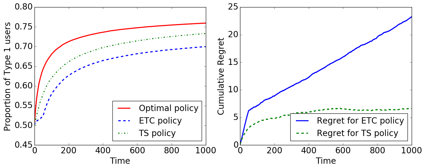
(a) $B_{1}=(b_{11}=0.9,b_{12}=0.4,b_{21}=0.2,b_{22}=0.6).$ Optimal policy is $(p=1,q=1)$ with asymptotic $z_{1}=0.80$.

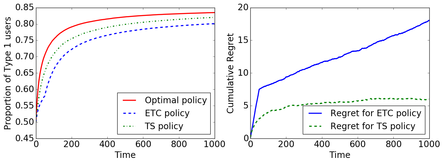
(b) $B_{2}=(b_{11}=0.9,b_{12}=0.4,b_{21}=0.6,b_{22}=0.7).$ Optimal policy is $(p=1,q=0)$ with asymptotic $z_{1}=0.86$.

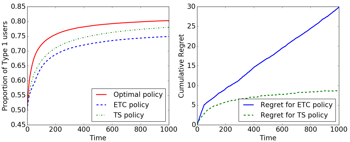
(c) $B_{3}=(b_{11}=0.7,b_{12}=0.1,b_{21}=0.3,b_{22}=0.5).$ Optimal policy is $(p=0,q=1)$ with asymptotic $z_{1}=0.83$.

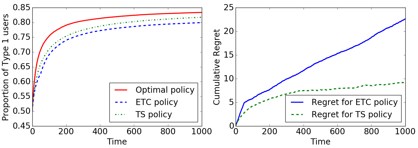
(d) $B_{4}=(b_{11}=0.7,b_{12}=0.1,b_{21}=0.6,b_{22}=0.6).$ Optimal policy is $(p=0,q=0)$ with asymptotic $z_{1}=0.86$.

Figure 2: Expected population proportion vs time (left) and cumulative regret vs time (right) for the ETC, TS, and the optimal policy that knows $B.$ The $B$ used for each of the plots and the optimal policy are also shown.

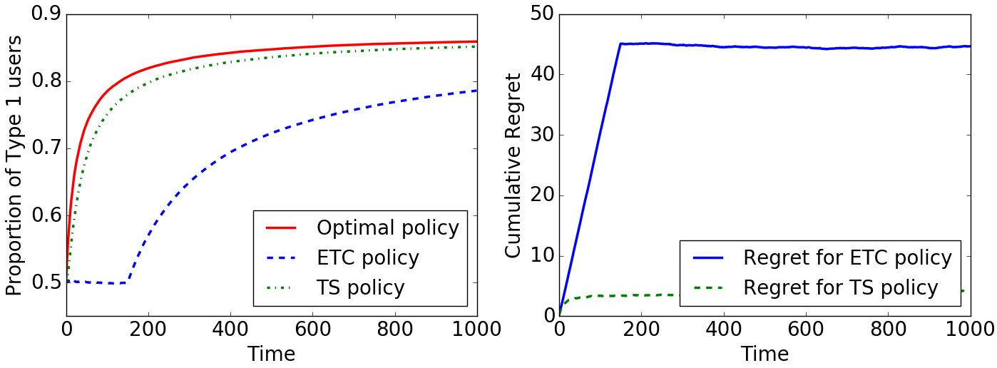
Figure 3: Expected population proportion vs time (left) and cumulative regret vs time (right) for the ETC, TS, and the optimal for $B_{sym}=(b_{11}=0.9,b_{12}=0.7,b_{21}=0.7,b_{22}=0.9)$

VI Preference Shaping with Constant Influence

In this section, we focus on the CID model in which the influence of the rewards on the population preferences is constant over time. Recall that the basic setup and reward structure remain the same as that of the DID model. However, the impact of the reward, $W_{t},$ accrued in each time slot changes. If a user of type $i$ arrives and gets a unit reward when $A_{t}=-i,$ or if it gets reward 0 if $A_{t}=i$ then one ball of type $i$ changes its color to the other color, $-i.$ The composition of the urn remains unchanged in the other two cases. Clearly, the ETC and Thompson sampling algorithms of, respectively, Algorithm 1 and Algorithm 2, can be used for the CID model without any change. In the following we will analyze their performance.

We first present the counterpart to Theorem 1. Assuming that $B$ is known, the trajectory of the fraction of type 1 population for policy $(p_{t},q_{t})=(p,q)$ is given by the following lemma.

Theorem 5.

For the CID model,for a policy $\pi$ such that $(p_{t},q_{t})=(p,q)$, the time evolution of the expected fraction of type 1 users is given by

$$z_{1}(t)=\frac{d_{2}}{d_{1}+d_{2}}+\left(z_{1}^{0}-\frac{d_{2}}{d_{1}+d_{2}}\right)e^{-t\frac{d_{1}+d_{2}}{N_{0}}}.$$ (11)

Here $d_{1}=p(1-b_{11})+(1-p)b_{12}$, $d_{2}=q(1-b_{22})+(1-q)b_{21}$ and $z_{1}(0)$ is the initial proportion of type 1 users.

We see that, with a fixed $(p,q),$ the asymptotic fraction of type 1 in the population for the CID model has the same value as that of the DID model. The difference though is in the rate at which the asymptotic value is approached. Since the expressions for the asymptotic proportions for CID and DID are the same, their optimizers would also be the same. Thus, it follows that the optimal policy for DID model as stated in Theorem 1, is also optimal for the CID model. This is counter-intuitive, since we expect that, because of the two-fold trade-off in the former case, the asymptotic value would be lesser than in the latter. An explicit proof is given in Appendix -J.

A comparison between the trajectories of $z(t)$ for the optimal $(p,q)$ for both the decreasing and the constant influence models is shown in Figure 4 for some sample values. We see that in the CID model, the asymptotic value is reached much more quickly due to the exponential decay term in (11) in Theorem 5 as opposed to polynomial in (7) for the DID model.

(a) $B_{1}=(b_{11}=0.7,b_{12}=0.1,b_{21}=0.2,b_{22}=0.5).$ Optimal policy is $(p=0,q=0).$

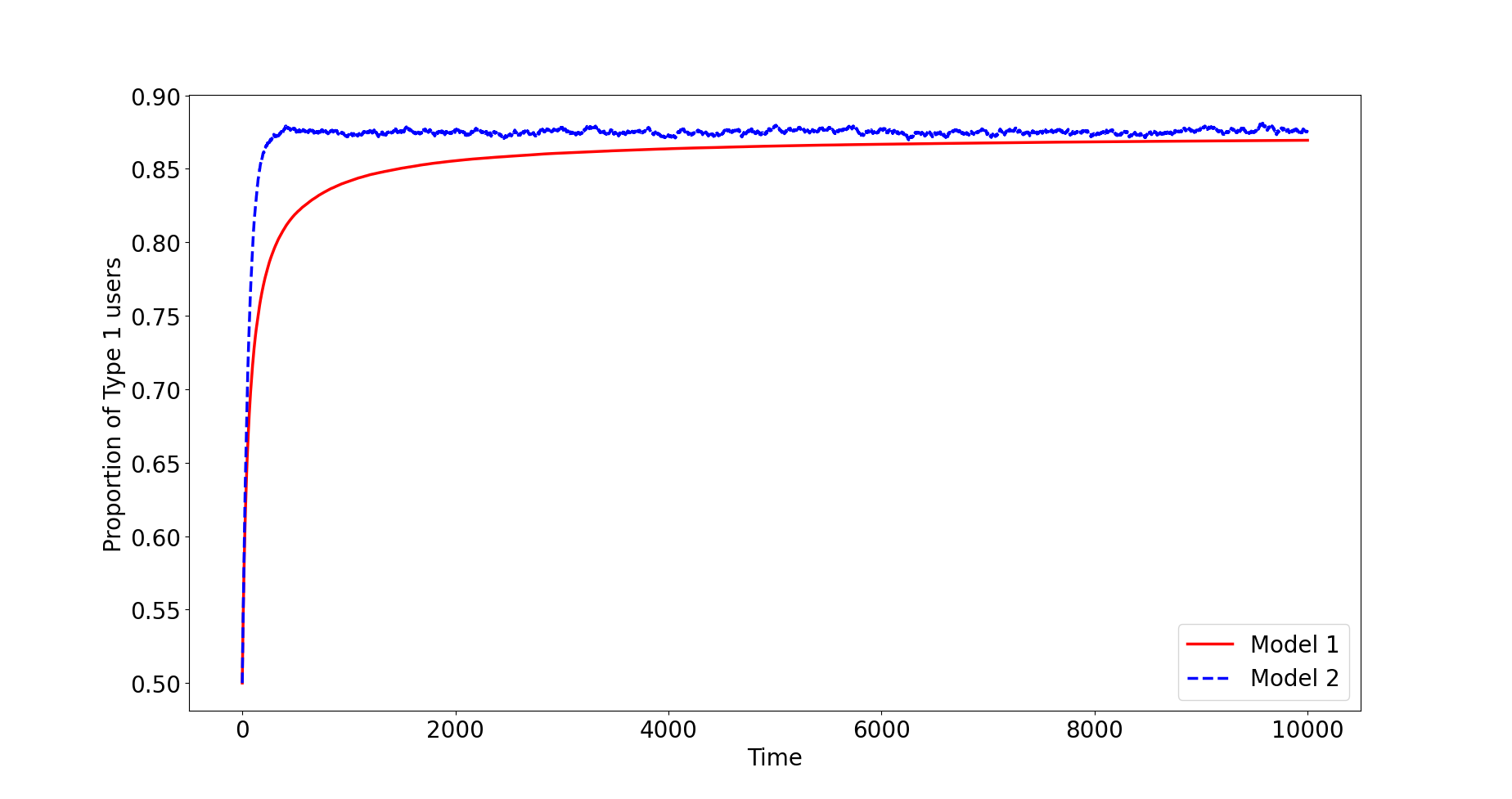
(b) $B_{2}=(b_{11}=0.9,b_{12}=0.7,b_{21}=0.7,b_{22}=0.9).$ Optimal policy is $(p=1,q=0).$

Figure 4: Expected population proportion vs time for optimal policies that knows $B.$ for DID model and the CID model. The $B$ used for each of the plots is also shown.

Next, we show that the other results, i.e., the bounds on the one-step regret, the cumulative regret for the special case of $b_{11}=b_{22}$ and $b_{12}=b_{21},$ and the cumulative regret for the Thompson sampling scheme of Algorithm 2, also carry over from the DID model to the CID model.

Lemma 4.

Let $\Delta_{1}:=|b_{11}+b_{12}-1|$ and $\Delta_{2}:=|b_{22}+b_{21}-1|$ and let $(p_{t},q_{t})$ be the strategy in slot $t.$ The general expression for regret for the CID model is

$$R_{t}(p_{t},q_{t}) =z_{1}(t)|\mathbbm{1}_{\{b_{11}+b_{12}-1>0\}}-p_{t}|\Delta_{1}+$$

$$\qquad(1-z_{1}(t))|\mathbbm{1}_{\{b_{21}+b_{22}-1<0\}}-q_{t}|\Delta_{2}$$

Note that the general expression for regret for the model presented in this section is same as the expression we obtained for the previous model in Lemma 2. Thus it follows from the above result that all regret bounds stated in Section V hold for the constant influence model.

Theorem 6.

1. For the special case of $b_{11}=b_{22}$ and $b_{12}=b_{22},$ the upper bound on the cumulative regret is given by (8).

2. The cumulative regret bound for the ETC algorithm (Algorithm 1) with population dynamics following CID model is given by (9).

3. The cumulative regret bound for the Thompson sampling algorithm (Algorithm 2) with population dynamics following CID model is given by (10).

VII Extensions

We consider two different extensions in this section.

VII-A Generalizing to $N$ arms

We now consider an MAB with $N$ arms and $N$ user types. As with the two-type case, the evolution of the population types is tracked using an urn that has balls of $N$ different colours. Following from the previous sections, $B[[b_{ij}]]$ is an $N\times N$ matrix of reward means, where $b_{ij}$ is the mean reward obtained when a user of type $i$ is shown arm $j.$ The mechanism for user arrival is the same as that in the two-arm case: Denoting the fraction of balls of color $i$ in the urn at time $t$ by $z_{i}(t),$ the user is of type of $i$ with probability $z_{i}(t).$ Furthermore, we consider the contextual bandit in which $S$ knows the type of the user.

We consider the following natural extension to the decreasing influence dynamics model for the two-arm case of Section III.

• If $A_{t}\neq X_{t}$ then $Z_{A_{t}}(t+1)=Z_{A_{t}}(t)+W_{t}$ and $Z_{X_{t}}(t+1)=Z_{X_{t}}(t)+1-W_{t}$. This update is exactly like the updates of the two-arm DID model of Section III.

• If $A_{t}=X_{t}$ then

  • If $W_{t}=1$ then $Z_{A_{t}}(t+1)=Z_{A_{t}}(t)+1$. This is also like in Section III.

  • If $W_{t}=0$ then $Z_{j}(t+1)=Z_{j}(t)+1$ where $j(\neq A_{t})$ is an arm chosen uniformly at random from the set of all arms excluding arm $A_{t}$. Note that for $N=2,$ this reduces to the two-arm DID model of Section III.

In each time step $t$, the MAB uses a randomised policy defined by an $N\times N$ stochastic matrix $P=[[p_{ij}]],$ where $p_{ij}$ is the probability that arm $A_{j}$ is shown to a user of type $i.$ As before, we will consider a contextual bandit where $S$ knows the type of the user before recommending. Further, we will also assume that $S$ knows the population profile determined by the number of balls of the different colors in the urn, i.e., $S$ knowns $Z(t)=[Z_{1}(t),Z_{2}(t),\ldots,Z_{N}(t)]^{T}$ for all $t.$ As before, we seek the optimal policy $P^{*}$ for maximizing $E[\Delta Z_{1}(t)|Z(t)].$ The following lemma gives us the optimal policy, the extension to Theorem 1.

Lemma 5.

The optimal policy $P^{*}$ for the $N$-arm decreasing influence dynamics model is given by

• For Row 1 of $P^{*}$ :

  • $P^{*}_{11}=1$ if $B_{11}>max(1-B_{12},\ldots,1-B_{1N})$

  • else $P^{*}_{1j}=1$ where $j=\arg\max_{k}(1-B_{1k})$

• For Row $i$ ($\neq 1$) of $P^{*}$ :

  • $P^{*}_{i1}=1$ if $B_{i1}>(1-B_{ii})/(N-1)$

  • $P^{*}_{ii}=1$ otherwise

We remark here that this policy is more generally applicable. For example, even if the population dynamics were changed as follows: for the case $A_{t}=X_{t}$ and $W_{t}=0,$ then choose $j$ with probability proportional to the $j$-type population instead of choosing uniformly at random, the optimal policy would be of a form similar to that in Lemma 5. This is because the derivation would still involve maximizing a convex combination like the one we see while proving the lemma (see the Appendix).

For the case when the matrix $B$ is unknown, once we have the expression for an optimal policy for the $N$-arm model (like the one in Lemma 5), we can apply Thompson sampling (with the optimal policy applied on a sampled matrix $\tilde{B}$ in each time slot instead of $B$) to maximize the proportion of type 1 users.

The optimal and Thompson sampling based strategies mentioned above have been simulated for the $N-$arms case and the trajectory of the type 1 population for a few example cases are shown in Figure 5. Even in the $N>2-$armed bandit examples, we observe that the Thompson sampling does not fall far behind the optimal trajectory and gives us a healthy majority of type 1 users ($\approx 80\%$ in all cases). We have not obtained analytic guarantees on the population trajectories for these cases, and a regret-based analysis remains open.

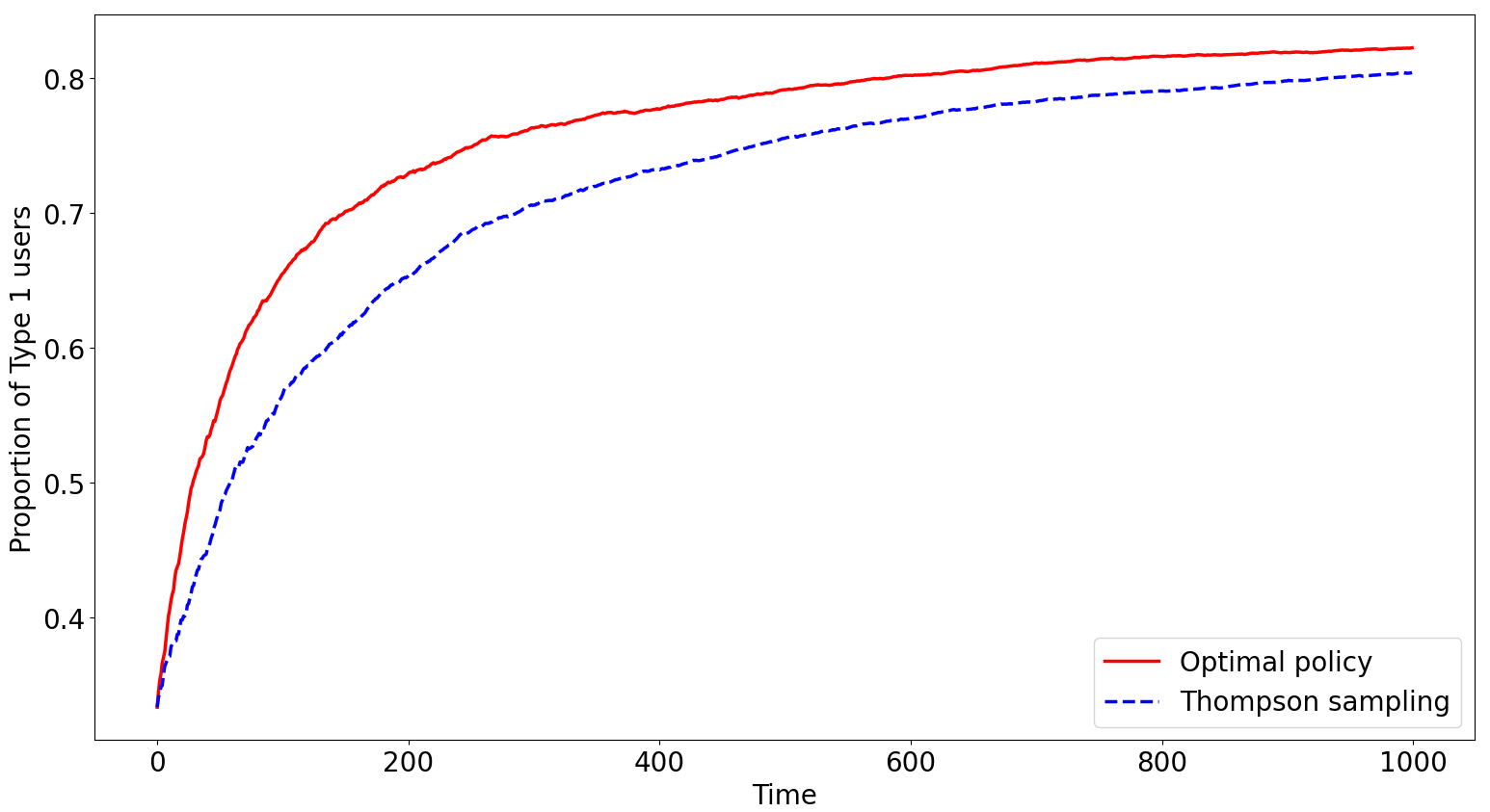
(a) Preference shaping with 3 arms. Matrix $B$ is $3\times 3$ with diagonal terms = 0.9 and off-diagonal terms = 0.7.

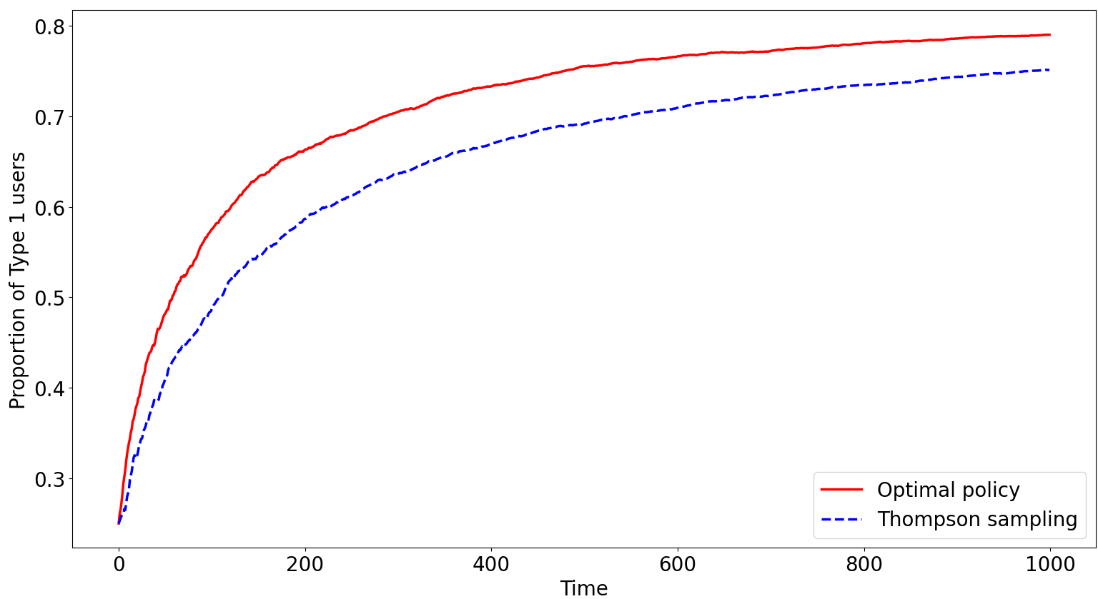
(b) Preference shaping with 4 arms. Matrix $B$ is $4\times 4$ with diagonal terms = 0.9 and off-diagonal terms = 0.6.

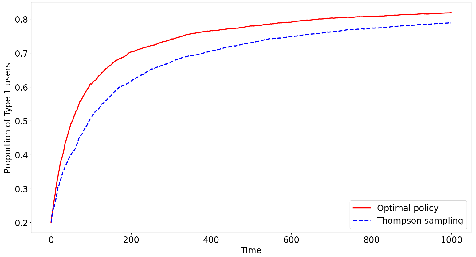
(c) Preference shaping with 5 arms. Matrix $B$ is $5\times 5$ with diagonal terms = 0.9 and off-diagonal terms = 0.7.

Figure 5: Expected population proportion vs time for optimal policy and Thompson sampling policy for $N-$arm case. The $N$ and $B$ used for each of the plots is also shown.

VII-B Two competing recommendation systems

Consider the same two-arm model as before, but we have two recommendation systems $S_{1}$ and $S_{2}$ instead of just one. Assume that $S_{1}$ is trying to maximize the number of type 1 users while $S_{2}$ is trying to achieve the opposite. Had the recommendation systems been alone, we saw that they may adopt optimal policies that recommend a disliked arm to a user. In real life, such an action might make the user dislike the recommendation system itself. Therefore, when multiple systems are present, we need to keep track of a “popularity” metric that measures how popular a particular system is among a certain type of user. In a time slot, a user either goes to be served by $S_{1}$ or $S_{2}$. The probability of a user going to a recommendation system is determined by the popularity of the system among users of the same type. The popularity of a system should increase on receiving a positive reward and decrease on receiving a negative (or zero) reward. We now make this more precise.

Competing recommendation systems (CRS): Define the popularity matrix $P^{t}=\begin{bmatrix}P_{11}^{t}&P_{12}^{t}\\ P_{21}^{t}&P_{22}^{t}\end{bmatrix}$.

The row number of an element represents the user type, and the column number represents the recommendation system. If a user of type $X_{t}$ arrives, it chooses to be served by the system $S_{1}$ with probability $\frac{P_{X_{t}1}^{t}}{P_{X_{t}1}^{t}+P_{X_{t}2}^{t}}$. For the case when the user goes with system $S_{1}$, we update the popularity matrix in the following way.

$$P_{X_{t}1}^{t+1} =P_{X_{t}1}^{t}+W_{t}$$ (12)

$$P_{X_{t}2}^{t+1} =P_{X_{t}2}^{t}+(1-W_{t})$$ (13)

where $W_{t}$ is the reward obtained after an arm is recommended by the system. This is similar to the population preference dynamics. The population of users is updated in the DID or the CID models from Section III. Thus we have both the population preference for arm and the population preference for the recommendation system interacting with the recommendations made and the rewards seen by the users.

In this setup of recommendation systems with opposing objectives, an interesting question is whether there are any equilibrium strategies that balance the popularity of the recommendation system, akin to market share, as well as their population preference shaping objectives. If the objective of $S_{1}$ and $S_{2}$ were to only increase their popularity, they would both follow the policy $(p=1,q=1)$. However, since the optimal population preference shaping policy might not always be $(p=1,q=1)$, each faces a tradeoff between their goals of increasing popularity and of preference shaping. In this preliminary study, we assume that each system is concentrating solely on preference shaping and ran some simulations. We note that depending on the structure of matrix $B$, we obtain two kinds of behaviours.

VII-B1 Case 1 (Uniform Population)

This is the case where the matrix $B$ is such that the optimal policy in Theorem 1 is either $(0,0)$ or $(1,1)$. Note that the optimal policy of $S_{1}$ and $S_{2}$ come out to be exactly the opposite of each other (i.e. if $(p^{*},q^{*})=(1,1)$ for $S_{1}$, then it is $(0,0)$ for $S_{2}$ and vice-versa).

In this case, the popularity of the same recommender system dominates in both type of user populations; see Fig. 6 and 9). In the former case, the optimal policy for $S_{1}$ is $(1,1)$. Here, $S_{1}$ clearly has no incentive to deviate from this policy since this policy increases both type 1 preferences and its own popularity among all users. At the end of 1000 time slots, therefore, we observe that a large fraction of the user population is using the services of $S_{1}.$ This makes the type 1 users the majority in the population. Note that this majority is still less than what it could have been had $S_{2}$ not been present. In Fig. 9, the opposite happens, i.e., $S_{2}$ dominates.

In both cases above, a large fraction of the population end up preferring one recommender over the other, regardless of their type.

VII-B2 Case 2 (Polarized Population)

This is the case where the matrix $B$ is such that the optimal policy in Theorem 1 is either $(0,1)$ or $(1,0)$.

In this case, the popularity of the different recommender system dominates in different type of user populations (See Fig. 7 and 8). Take the former case where the optimal policy for $S_{1}$ is $(1,0)$. At the end of 1000 time slots, we observe that the vast majority of the user population of type 1 is using the services of $S_{1}$, and those of type 2, are using the services of $S_{2}$. In the next figure, the opposite happens.

In both cases, we see that each type of user dominates the user base of different recommendation systems.

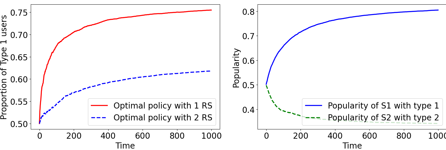
Figure 6: Expected population proportion vs Time (left) and Popularity vs Time (right) for optimal policies for $B_{1}=(b_{11}=0.9,b_{12}=0.4,b_{21}=0.2,b_{22}=0.6).$

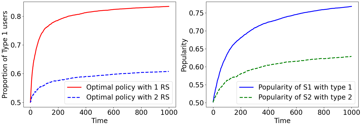
Figure 7: Expected population proportion vs Time (left) and Popularity vs Time (right) for optimal policies for $B_{2}=(b_{11}=0.7,b_{12}=0.5,b_{21}=0.6,b_{22}=0.8).$

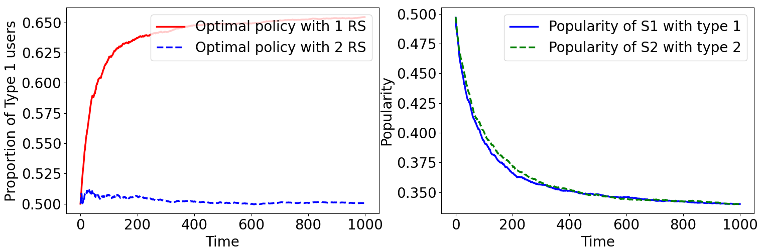
Figure 8: Expected population proportion vs Time (left) and Popularity vs Time (right) for optimal policies for $B_{3}=(b_{11}=0.6,b_{12}=0.2,b_{21}=0.2,b_{22}=0.6).$

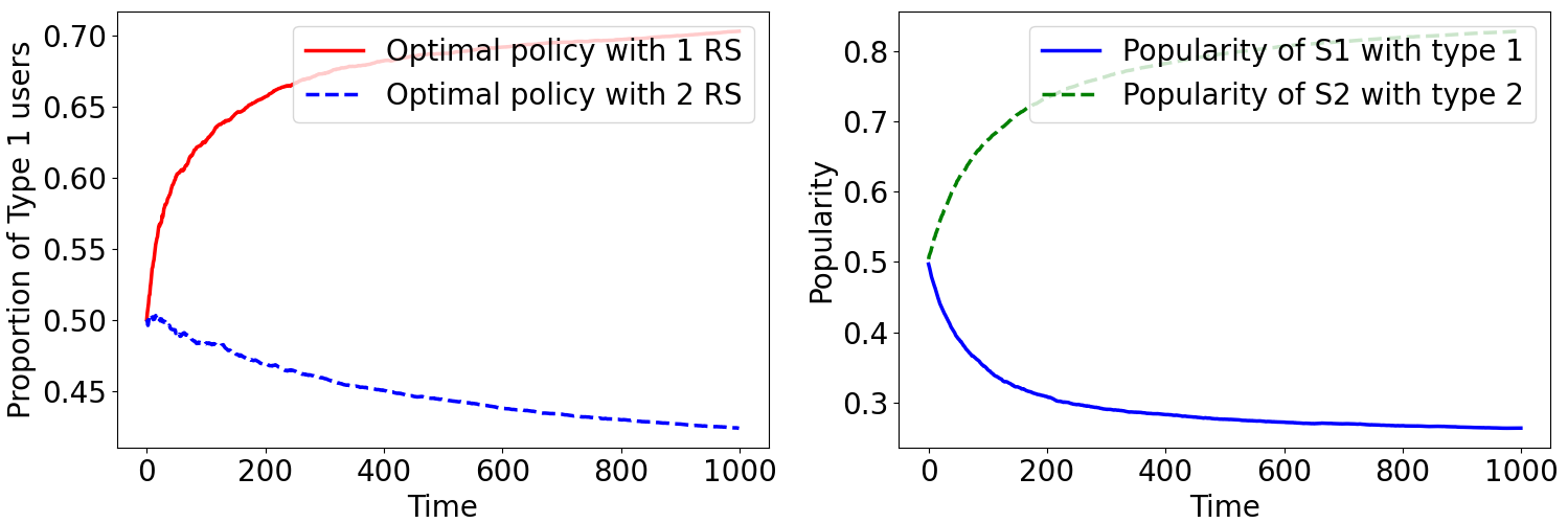
Figure 9: Expected population proportion vs Time (left) and Popularity vs Time (right) for optimal policies for $B_{4}=(b_{11}=0.7,b_{12}=0.1,b_{21}=0.3,b_{22}=0.9).$

VIII Concluding Remarks

In this paper, we considered the problem of preference shaping in a user population using multi-armed bandit algorithms. We presented a simplified version of this problem for two arms and two corresponding user types, where the preferences of a user change in response to the random Bernoulli reward obtained (can be thought of as like/dislike) in response to the recommendation. We found how the population behaves if the recommender follows a certain policy and hence found the optimal policy to be followed if the Bernoulli reward means are known. We then used Explore-then-Commit and Thompson sampling algorithms to get policies that approach the optimal in the case when the Bernoulli reward means are unknown. We also extended these algorithms for the cases when we have $N$ arms or more than one recommender.

Clearly both the DID and the CID models can be generalised in many ways. For example, in the DID model, the composition of the urn could be changed by adding $K$ balls to the urn at every step of which $m$ balls are of one color and $K-m$ balls are of the other color. The rate at which the influence decreases can be tuned using different $K$ and $m.$ The theory for this would be similar to that derived in this paper. Similarly, in the CID model, the composition of the urn could be changed with probability $\beta$ in every step. Once again, a suitable choice of $\beta$ will determine the degree of change in every step.

There are two possible directions in which one can further extend our models and results. Firstly, we can generalize by evolving the type of a user via an underlying Markov Decision Process rather than the urn model that we considered. Note that mapping our model to an MDP requires an MDP where the transition probabilities are affected by the rewards that are accrued. Since many recommendation systems may not have an estimate about the composition of the user population, one can further extend this to the case where the type of a user is not visible.

A second direction would be to keep the existing two recommendation system model and introduce different rewards for opinion shaping and popularity. This maps to the problem that a real-life recommendation system may have between, say PR/advertising money (opinion shaping) and maintaining popularity among its current user base. This model would provide a trade-off between the algorithms discussed in [19] and the ones discussed in this paper, and it would be interesting to see whether we arrive at some equilibrium strategy and population distribution for such a setting.

Understanding and modeling the interaction between a recommender system’s learning algorithm and the preferences of the user population is becoming increasingly important. Specifically, the ‘exploration’ part of the algorithm could ‘expose’ the user to possibilities that in turn might make them to also explore and possibly start preferring other options. Similarly, the exploitation part of the algorithm may reinforce the users’s possibly weak preferences. We believe that the models that we have presented here could be used in understanding and modeling such behaviour.

-A Comparison between regret definitions

The commonly used definition of regret would compare the difference in the population trajectories of the optimal and the candidate policies directly. Specifically, let $Z_{1}^{*}(t)$ be the trajectory of the population of type 1 balls in the urn when the optimal policy is applied and let $Z_{1}(t)$ be the population when the candidate policy is applied. Thus the following definition of regret, denoted by $R_{t}^{{}^{\prime}},$ is more like what is commonly used in the literature when the objective is to learn the best arm.

$$R_{t}^{{}^{\prime}}=E[\Delta Z_{1}^{*}(t)|Z_{1}^{*}(t)]-E[\Delta Z_{1}(t)|Z_{1}(t)]$$ (14)

Let us now compare this with our definition of regret $R_{t}$ in (5). Taking the difference between the two definitions gives us

$$R_{t}-R_{t}^{{}^{\prime}} =E[\Delta Z_{1}^{*}(t)|Z_{1}(t)]-E[\Delta Z_{1}^{*}(t)|Z_{1}^{*}(t)]$$

$$=(z_{1}(t)-z_{1}^{*}(t))\left((b_{11}+b_{12}-1)^{+}+(1-b_{12})\right.$$

$$\hskip 36.135pt\left.-(1-b_{21}-b_{22})^{+}-b_{21}\right),$$

where $x^{+}=\max(x,0).$ In the second equality above we have used the optimal policy for the DID model obtained in Theorem 1 to derive the expressions for $E[\Delta Z_{1}(t)|Z_{1}(t)]$. (From the results in Section VI this is also applicable to CID model.) We know, by definition, that the trajectory followed by the optimal policy is always above that followed by any other policy. Therefore, $(z_{1}(t)-z_{1}^{*}(t))<0$. Thus the lemma below follows immediately.

Lemma 6.

$R_{t}^{{}^{\prime}}$ is bounded above by the regret $R_{t}$ if and only if $(b_{11}+b_{12}-1)^{+}+(1-b_{12})\leq(1-b_{21}-b_{22})^{+}+b_{21}$.

-B Proof of Theorem 1

The expression for expected increase in type 1 balls in time slot $t$ is given by

$$E\left[\Delta Z_{1}^{\pi}(t)|z_{1}(t)\right] =P(\Delta Z_{1}^{\pi}(t)=1|z_{1}(t))$$

$$=\sum_{i=1,2}P(X_{t}=i|z_{1}(t))P(\Delta Z_{1}^{\pi}(t)=1,$$

$$\qquad|X_{t}=i,z_{1}(t))$$

$$=z_{1}(t)(p_{t}(b_{11})+(1-p_{t})(1-b_{12}))+$$

$$\qquad(1-z_{1}(t))((1-q_{t})(b_{21})+(q_{t})(1-b_{22}))$$

$$=z_{1}(t)(p_{t}(b_{11}+b_{12}-1)+1-b_{12})+$$

$$\qquad(1-z_{1}(t))(q_{t}(1-b_{22}-b_{21})+b_{21})$$

The last expression above is to be maximized over all possible $(p_{t},q_{t})$. This is a simple linear expression in terms of both these variables. Hence, since $z_{1}(t),1-z_{1}(t)>0$, $E[\Delta Z_{1}^{\pi}(t)|z_{1}(t)]$ is maximized when

$$(p_{t},q_{t})=(\mathbbm{1}_{\{b_{11}+b_{12}-1>0\}},\mathbbm{1}_{\{1-b_{21}+b_{22}>0\}}).$$

which proves the theorem ∎

-C Proof of Lemma 1

For $d_{1}$ and $d_{2}$ as defined in the statement of the lemma, and referring to the proof of Lemma 1, we get:

$$E[\Delta Z_{1}^{\pi}(t)|z_{1}(t)] =z_{1}(t)(1-d_{1})+(1-z_{1}(t))d_{2}$$

This corresponds to o.d.e

$$\dot{Z_{1}^{\pi}}(t)=\frac{Z_{1}(t)(1-d_{1})+(N_{0}+t-Z_{1}(t))d_{2}}{N_{0}+t}$$

We can now substitute $Z_{1}^{\pi}(t)=(N_{0}+t)z_{1}(t)$ to get the o.d.e.

$$\dot{z_{1}}(t)=\frac{d_{2}-(d_{1}+d_{2})z_{1}(t)}{N_{0}+t}$$

Solving this o.d.e gives us the desired result. ∎

-D Proof of Theorem 2

The proportion $\frac{d_{2}}{d_{1}+d_{2}}$ is to be maximised over the variables $(p,q)$. Since $d_{1}$ is only a function of $p$, we first minimize that with respect to $p$ since it is in the denominator.

$$p^{*} =\arg\min_{p}\ d_{1}$$

$$=\arg\min_{p}\ p(1-b_{11})+(1-p)b_{12}$$

$$=\arg\min_{p}\ p(1-b_{11}-b_{12})+b_{12}$$

$$=\mathbbm{1}_{\{b_{11}+b_{12}-1>0\}}$$

Now, $d_{2}$ (which depends only on $q$) appears both in the numerator and the denominator. But we can use the easily verifiable fact that $\frac{d_{2}}{d_{1}+d_{2}}$ is a strictly increasing function of $d_{2}$. This means maximizing $d_{2}$ also maximizes the proportion.

$$q^{*} =\arg\max_{q}\ d_{2}$$

$$=\arg\max_{q}\ q(1-b_{22})+(1-q)b_{21}$$

$$=\arg\max_{q}\ q(1-b_{22}-b_{21})+b_{21}$$

$$=\mathbbm{1}_{\{b_{22}+b_{21}-1<0\}}$$

We see that $(p^{*},q^{*})$ derived here indeed match with the results in Lemma 1

∎

-E Proof of Lemma 2

We know that:

$$\Delta Z^{\pi}_{1}(t) =W_{t}\mathbbm{1}_{A_{t}=1}+(1-W_{t})\mathbbm{1}_{A_{t}=2}$$

$$=\tilde{b}_{11}\mathbbm{1}_{A_{t}=1,X_{t}=1}+\tilde{b}_{21}\mathbbm{1}_{A_{t}=1,X_{t}=2}+$$

$$\qquad(1-\tilde{b}_{12})\mathbbm{1}_{A_{t}=2,X_{t}=1}+(1-\tilde{b}_{22})\mathbbm{1}_{A_{t}=2,X_{t}=2}$$

where $\tilde{b}_{ij}$ are independent samples of the Bernoulli rewards with the respective means as $b_{ij}$.

Therefore,

$$E[\Delta Z^{\pi}_{1}(t)|z_{1}(t)] =b_{11}z_{1}(t)p_{t}+b_{21}(1-z_{1}(t))(1-q_{t})+$$

$$\qquad(1-b_{22})(1-z_{1}(t))q_{t}+$$

$$\qquad(1-b_{21})z_{1}(t)(1-p_{t})$$

$$=z_{1}(t)p_{t}(b_{11}+b_{12}-1)+$$

$$\qquad(1-z_{1}(t))q_{t}(1-b_{22}-b_{21})+$$

$$\qquad b_{21}(1-z_{1}(t))+(1-b_{21})z_{1}(t)$$

For the optimal policy, the same expression becomes:

$$E[\Delta Z^{*}_{1}(t)|z_{1}(t)] =z_{1}(t)\mathbbm{1}_{\{b_{11}+b_{12}-1>0\}}(b_{11}+b_{12}-1)+$$

$$\qquad(1-z_{1}(t))\mathbbm{1}_{\{b_{21}+b_{22}-1<0\}}(1-b_{22}-b_{21})+$$

$$\qquad b_{21}(1-z_{1}(t))+(1-b_{21})z_{1}(t)$$

Substituting these results in the definition 3, we get :

$$R_{t}^{\pi} =E[\Delta Z_{1}^{*}(t)-\Delta Z_{1}^{\pi}(t)|Z_{1}^{*}(t)=Z_{1}^{\pi}(t)]$$

$$=z_{1}(t)(\mathbbm{1}_{\{b_{11}+b_{12}-1>0\}}-p_{t})(b_{11}+b_{12}-1)+$$

$$\qquad(1-z_{1}(t))(\mathbbm{1}_{\{b_{21}+b_{22}-1<0\}}-q_{t})(1-b_{21}-b_{22})$$

Since $0\leq p_{t},q_{t}\leq 1$, it means that $(\mathbbm{1}_{\{b_{11}+b_{12}-1>0\}}-p_{t})(b_{11}+b_{12}-1)$ and $(\mathbbm{1}_{\{b_{21}+b_{22}-1<0\}}-q_{t})(1-b_{21}-b_{22})$ are always positive. This proves the desired result. ∎

-F Proof of Lemma 3

The expression for $R_{explore}$ is obtained by substituting $(p_{t},q_{t})=(0.5,0.5)$ in the regret formula of Lemma 2 and summing from $t=1$ to $t=m$.

The expression for $R_{commit}$ is obtained by substituting $(p_{t},q_{t})=(\mathbbm{1}_{\{\hat{b}_{11}+\hat{b}_{12}-1>0\}},\mathbbm{1}_{\{\hat{b}_{22}+\hat{b}_{21}-1<0\}})$ in the regret formula of lemma 2 and summing from $t=m$ to $t=T$. ∎

-G Proof of Theorem 3

For $b_{11}=b_{22}$ and $b_{12}=b_{21}$, we get

$$R_{explore} =\frac{m\Delta_{1}}{2}$$

$$R_{commit} =p_{err}(T-m)\Delta_{1}$$

The term $p_{err}$ can be bounded in the following way:

$$p_{err} =P((\hat{b}_{11}+\hat{b}_{12}-1)(b_{11}+b_{12}-1)<0)$$ (15)

$$\leq P(|\hat{b}_{11}+\hat{b}_{12}-b_{11}-b_{12}|>\Delta_{1})$$ (16)

This is because the event in 15 is a subset of the event in 16.

Now, we know that Bernoulli random variables are $1/2-$sub-Gaussian. Since we show arm 1 and 2 with equal probability in the exploration phases, the expected number of times $b_{11}$ and $b_{12}$ are sampled is $m/2$ for each of the arms. This implies that $\hat{b}_{11}-b_{11}$ is $1/\sqrt{m/2}-$sub-Gaussian, which in turn implies that $\hat{b}_{11}+\hat{b}_{12}-b_{11}-b_{12}$ is $2/\sqrt{m}-$sub-Gaussian. Therefore we can use the Hoeffding bounds on sub-Gaussian random variables to further put a more useful bound on $p_{err},$ i.e.,

$$p_{err}\leq e^{-m\Delta_{1}^{2}/8}.$$

Therefore, we get a $\Delta_{i}$ dependent bound on the regret to be

$$R_{explore}+R_{commit}\leq m\Delta_{1}/2+(T-m)\Delta_{1}e^{-m\Delta_{1}^{2}/8}.$$

∎

-H Proof of Theorem 4

Using Lemma 2, the expression for the regret $R_{t}$ in time slot $t$ for Thompson sampling becomes:

$$R_{t}=z_{1}(t)p^{err}_{t}\Delta_{1}+(1-z_{1}(t))q^{err}_{t}\Delta_{2}$$

where

$$p^{err}_{t} =P((\tilde{b}_{11}^{t}+\tilde{b}_{12}^{t}-1)(b_{11}+b_{12}-1)<0)$$

$$q^{err}_{t} =P((\tilde{b}_{22}^{t}+\tilde{b}_{21}^{t}-1)(b_{22}+b_{21}-1)<0)$$

Here, the variables $\tilde{b}_{ij}^{t}$ denote the sampled matrix elements based on the $Beta(\alpha_{ij},\beta_{ij})$ distribution at that time.

Let us now put a bound on $p^{err}_{t}$.

$$p^{err}_{t} \leq P(|\tilde{b}_{11}^{t}+\tilde{b}_{12}^{t}-b_{11}-b_{12}|>\Delta_{1})$$

$$\leq\frac{Var(\tilde{b}_{11}^{t}+\tilde{b}_{12}^{t})}{\Delta_{1}^{2}}$$

where the second inequality is a direct application of Chebyschev’s inequality.

Since $\tilde{b}_{11}^{t}$ and $\tilde{b}_{12}^{t}$ are independently sampled, we have:

$$Var(\tilde{b}_{11}^{t}+\tilde{b}_{12}^{t}) =\frac{\alpha_{11}^{t}\beta_{11}^{t}}{(\alpha_{11}^{t}+\beta_{11}^{t})^{2}(\alpha_{11}^{t}+\beta_{11}^{t}+1)}$$

$$+\frac{\alpha_{12}^{t}\beta_{12}^{t}}{(\alpha_{12}^{t}+\beta_{12}^{t})^{2}(\alpha_{12}^{t}+\beta_{12}^{t}+1)}$$

where we have used the expression for the variance of Beta distributed random variables.

Let us assume that $x_{ij}^{t}=\frac{\alpha_{ij}^{t}}{\alpha_{ij}^{t}+\beta_{ij}^{t}}$. Substituting these in the expression for the variance, we get,

$$Var(\tilde{b}_{11}^{t}+\tilde{b}_{12}^{t}) =\frac{x_{11}^{t}(1-x_{11}^{t})}{\alpha_{11}^{t}+\beta_{11}^{t}+1}+\frac{x_{12}^{t}(1-x_{12}^{t})}{\alpha_{12}^{t}+\beta_{12}^{t}+1}$$

$$\leq\frac{1}{4}\left(\frac{1}{\alpha_{11}^{t}+\beta_{11}^{t}+1}+\frac{1}{\alpha_{12}^{t}+\beta_{12}^{t}+1}\right)$$

$$=\frac{1}{4}\frac{\alpha_{11}^{t}+\beta_{11}^{t}+\alpha_{12}^{t}+\beta_{12}^{t}+2}{(\alpha_{11}^{t}+\beta_{11}^{t}+1)(\alpha_{12}^{t}+\beta_{12}^{t}+1)}$$

Now, $\alpha_{11}^{t}+\beta_{11}^{t}+\alpha_{12}^{t}+\beta_{12}^{t}$ is the expected number of times a type 1 user appears. Out of that, let $f_{1}$ be the fraction of the time arm 1 was recommended. Therefore, by definition, $z^{*}t\geq\alpha_{11}^{t}+\beta_{11}^{t}+\alpha_{12}^{t}+\beta_{12}^{t}$ and $(\alpha_{11}^{t}+\beta_{11}^{t}+1)(\alpha_{12}^{t}+\beta_{12}^{t}+1)\approx(f_{1}t)((1-f_{1})t)$ Substituting these observations, we get:

$$Var(\tilde{b}_{11}^{t}+\tilde{b}_{12}^{t}) \leq\frac{z^{*}t}{4(f_{1}t)((1-f_{1})t)}$$

$$=\frac{z^{*}}{4f_{1}(1-f_{1})t}$$

This gives us:

$$p^{err}_{t}\leq\frac{z^{*}}{4\Delta_{1}^{2}f_{1}(1-f_{1})t}$$

Therefore,

$$R_{t}\leq\frac{z^{*}}{t}\left(\frac{z_{1}(t)}{4\Delta_{1}f_{1}(1-f_{1})}+\frac{1-z_{1}(t)}{4\Delta_{2}f_{2}(1-f_{2})}\right)$$

where $f_{2}$ is the fraction of time arm 2 was recommended when a user of type 2 showed up. By definition, $z^{*}\geq z_{1}(t),1-z_{1}(t)$. Therefore, using this and summing over $t$, we get

$$R_{[1:T]}^{Thomp}\leq\frac{(z^{*})^{2}}{4}\left(\frac{1}{f_{1}(1-f_{1})\Delta_{1}}+\frac{1}{f_{2}(1-f_{2})\Delta_{2}}\right)\sum_{t=1}^{T}\frac{1}{t}.$$

This leads to the desired result by bounding the summation by an integral.

∎

-I Proof for Lemma 4

In the proof of the Lemma 5, we had obtained :

$$E[Z_{1}(t+1)-Z_{1}(t)|Z_{1}(t)] =p_{2}-p_{1}$$

$$\implies E[\Delta Z_{1}(t)|z_{1}(t)] =z_{1}(t)(p(1-b_{11})+(1-p)b_{12})+$$

$$\qquad(1-z_{1}(t))(q(1-b_{22})+$$

$$\qquad(1-q)b_{21})$$

$$=z_{1}(t)p(1-b_{11}-b_{12})+$$

$$\qquad(1-z_{1}(t))q(1-b_{21}-b_{22})+$$

$$\qquad z_{1}(t)b_{12}+(1-z_{1}(t))b_{21}$$

Similarly, we get (since the optimal policy is same as the one given in Lemma 1) :

$$E[\Delta Z^{*}(t)|z_{1}(t)] =z_{1}(t)p^{*}(1-b_{11}-b_{12})+$$

$$\qquad(1-z_{1}(t))q^{*}(1-b_{21}-b_{22})+$$

$$\qquad z_{1}(t)b_{12}+(1-z_{1}(t))b_{21}$$

where $p^{*}=\mathbbm{1}_{\{b_{11}+b_{12}-1>0\}}$ and $q^{*}=\mathbbm{1}_{\{b_{22}+b_{21}-1<0\}}$.

Using the expression in definition 3 for regret directly gives us the desired result. ∎

-J Proof of Lemma 5

From the model, we know that

$$Z_{1}(t+1) =Z_{1}(t)-1\ \textrm{w.p}\ p_{1}=Z_{1}(t)d_{1}/N_{0}$$

$$=Z_{1}(t)+1\ \textrm{w.p}\ p_{2}=(1-Z_{1}(t)/N_{0})d_{2}$$

$$=Z_{1}(t)\ \textrm{w.p}\ 1-p_{1}-p_{2}$$

Therefore,

$$E[Z_{1}(t+1)-Z_{1}(t)|Z_{1}(t)] =p_{2}-p_{1}$$

$$=d_{2}-\frac{Z_{1}(t)}{N_{0}}\ (d_{1}+d_{2})$$

Thus gives us the corresponding o.d.e. as

$$\dot{Z}_{1}(t)=d_{2}-\frac{Z_{1}(t)}{N_{0}}\ (d_{1}+d_{2})$$

Solving for $Z_{1}$ and dividing the solution by $N_{0}$ gives us the required solution for $z_{1}(t)$. ∎

-K Proof of Lemma 5

For this model, we have

$$E[\Delta Z_{1}(t)|\bar{z}(t)] =P(\Delta Z_{1}(t)=1|\bar{z}(t))$$

$$=z_{1}(t)(P_{11}B_{11}+\sum_{j=2}^{N}P_{1j}(1-B_{1j}))+$$

$$\qquad\sum_{i=2}^{N}z_{i}(t)\left(P_{i1}B_{i1}+\frac{P_{ii}(1-B_{ii})}{N-1}\right)$$

Since $z_{i}(t)$ are known constants and we are optimizing over all $P_{ij}$ such that $\sum_{j}P_{ij}=1$, we observe that each term in brackets that is multiplying $z_{i}(t)$ is a convex combination of terms containing $B_{ij}$. To maximize a convex combination, we set the coefficient of the largest term to be 1. This gives us the stated result. ∎

-L Simulation details

All of the regret and population proportion curves generated for comparison of ETC and TS policies in the context of an unknown rewards matrix have been done after averaging over 1000 simulations and letting each of the simulations run for 1000 time steps.

In each simulation, the type of the arriving user is sampled from a Bernoulli distribution with the probability of type 1 user arriving being $z_{1}(t)$ and the user being type 2 otherwise. The arm is then chosen according to the prescribed policy (ETC, TS or optimal). The arms and type together specify an element of the rewards matrix. The reward is thus sampled from a Bernoulli RV with this element as the mean. The population of users is updated according to the CID or DID model (as specified in Section III) and then we move on to the next time step where the above sequence of events is repeated.

References

- [1] S. Bubeck and N. Cesa-Bianchi, “Regret analysis of stochastic and nonstochastic multi-armed bandit problems,” Foundations and Trends in Machine Learning, vol. 5, no. 1, 2012.
- [2] T. Lattimore and C. Szepesv´ari, Bandit Algorithms. Preprint, 2018. https://tor-lattimore.com/downloads/book/book.pdf
- [3] A. Slivkins, “Introduction to multi-armed bandits,” 2019.
- [4] J. Langford and T. Zhang, “The epoch-greedy algorithm for contextual multi-armed bandits,” in Advances in Neural Information Processing Systems. NIPS, Dec. 2007, pp. 1–8.
- [5] V. S. Borkar, J. Nair, and N. Sanketh, “Manufacturing consent,” IEEE Transactions on Automatic Control, vol. 60, no. 1, pp. 104–117, January 2015.
- [6] S. Eshghi, V. Preciado, S. Sarkar, S. Venkatesh, Q. Zhao, R. D’Souza, and A. Swami, “Spread, then target, and advertise in waves: Optimal budget allocation across advertising channels,” IEEE Transactions on Network Science and Engineering, vol. 7, no. 2, pp. 750–763, October 2018.
- [7] M. Goyal, D. Chatterjee, N. Karamchandani, and D. Manjunath, “Maintaining ferment,” in Proceedings of IEEE CDC, 2019, pp. 5217–5222.
- [8] K. Palda, “The measurement of cumulative advertising effects,” The Journal of Business, vol. 38, pp. 162–179, 1965.
- [9] D. Cowling, M. Modayil, and C. Stevens, “Assessing the relationship between ad volume and awareness of a tobacco education media campaign,” Tobacco Control, 2010. ncbi.nlm.nih.gov/pmc/articles/PMC2976530/pdf/tc030692.pdf
- [10] R. A. Holley and T. M. Liggett, “Ergodic theorems for weakly interacting infinite systems and the voter model,” Annals of Probability, vol. 3, no. 4, pp. 643–663, August 1975.
- [11] J. Gittins, K. Glazebrook, and R. Weber, Multi-armed Bandit Allocation Indices, 2nd ed. New York: John Wiley and Sons, 2011.
- [12] C. C. Wang, S. Kulkarni, and H. V. Poor, “Bandit problems with side observations,” IEEE Transactions on Automatic Control, vol. 50, no. 3, pp. 338–355, 2005.
- [13] O. Besbes, Y. Gur, and A. Zeevi, “Stochastic multi-armed bandit problem with non-stationary rewards,” Stochastic Systems, vol. 9, no. 4, pp. 319–416, December 2019.
- [14] N. Levine, K. Crammer, and S. Mannor, “Rotting bandits,” in Neural Information Processing Systems, 2017, pp. 3077–3086.
- [15] N. Immorlica and R. D. Kleinberg, “Recharging bandits,” in Foundations of Computer Science, 2018.
- [16] R. Meshram, D. Manjunath, and A. Gopalan, “On the whittle index for restless multiarmed hidden markov bandits,” IEEE Transactions on Automatic Control, vol. 63, no. 9, pp. 3046–3053, September 2018.
- [17] R. Meshram, A. Gopalan, and D. Manjunath, “Optimal recommendation to users that react: Online learning for a class of pomdps,” in Proceedings of IEEE CDC, 2016.
- [18] T. Fiez, S. Sekar, and L. J. Ratliff, “Multi-armed bandits for correlated markovian environments with smoothed reward feedback,” 2019.
- [19] V. Shah, J. Blanchet, and R. Johari, “Bandit learning with positive externalities,” in Proceedings of NeurIPS, 2018. https://arxiv.org/pdf/1802.05693.pdf
- [20] Q. Wu, N. Iyer, and H. Wang, “Learning contextual bandits in a non-stationary environment,” in Proceedings of the 41st ACM SIGIR Conference, June 2018, pp. 495–504. https://doi.org/10.1145/3209978.3210051
- [21] G. Pólya, “Sur quelques points de la théorie des probabilités,” Annals of Inst. H. Poincaré, vol. 1, no. 2, pp. 117–161, 1930.
- [22] R. Pemantle, “A survey of random processes with reinforcement,” Probabability Surveys, vol. 4, pp. 1–79, 2007.
- [23] H. Robbins and S. Monro, “A stochastic approximation method,” The Annals of Mathematical Statistics, vol. 22, no. 3, 1951.
- [24] B. Kumar, V. S. Borkar, and A. Shetty, “Bounds for tracking error in constant stepsize stochastic approximation,” 2018. arXiv:1802.07759