Viable Wormhole Solutions in Modified Gauss-Bonnet Gravity

Abstract

In this paper, we use the embedding class-I technique to examine the effect of charge on traversable wormhole geometry in the context of $f(\mathcal{G})$ theory, where $\mathcal{G}$ is the Gauss-Bonnet term. For this purpose, we consider static spherical spacetime with anisotropic matter configuration to investigate the wormhole geometry. The Karmarkar condition is used to develop a shape function for the static wormhole structure. Using this developed shape function, we construct a wormhole geometry that satisfies all the required constraints and connects asymptotically flat regions of the spacetime. To analyze the existence of traversable wormhole geometry, we evaluate the behavior of energy conditions for various models of this theory. This study reveals that viable traversable wormhole solutions exist in this modified theory.

Keywords: Wormhole; $f(\mathcal{G})$ theory; Karmarkar condition; Stability.
PACS: 04.50.Kd; 03.50.De; 98.80.Cq; 04.40.Nr.

1 Introduction

The mysterious characteristics of our universe raise marvelous questions for the research community. The presence of hypothetical structures is assumed as the most controversial issue that yields the wormhole (WH) structure. A WH is a hypothetical concept that refers to a shortcut or a tunnel through spacetime. The basic idea behind a WH is that it connects two separate points in spacetime, allowing for faster-than-light travel. A WH that connects different parts of the separate universe is called an inter-universe WH, but an intra-universe WH joins distinct parts of the same universe. The notion of a WH was first proposed in 1916 by the physicist Flamm [1]. He used the Schwarzschild solution to develop WH structure. Later, Einstein and Rosen [2] presented the concept of Einstein-Rosen bridge, which examined that spacetime can be connected by a tunnel-like structure, allowing for a shortcut or bridge between two distinct regions of spacetime.

According to Einstein’s theory of general relativity (GR), WHs can exist if there is enough mass and energy to warp spacetime in a specific way. They are also believed to be highly unstable and may require exotic matter (which contradicts energy conditions) with negative energy density to maintain their structure. However, scientists continue to study the concept of WHs and their implications for understanding the universe. According to Wheeler [3], Schwarzschild WH solutions are not traversable due to the presence of strong tidal forces at WH throat and the inability to travel in two directions. Furthermore, the throat of WH rapidly expands and then contracts, preventing access to anything. However, it is analyzed that WHs would collapse immediately after the formation [4]. The possibility of a feasible WH is being challenged due to the enormous amount of exotic matter. Thus, a viable WH structure must have a minimum amount of exotic matter. Morris and Thorne [5] proposed the first traversable WH solution.

The study of wormhole shape functions (WSFs) is one of the most interesting subjects in traversable WH geometry. Shape functions play a crucial role in determining the properties and behavior of traversable WHs. They are mathematical functions that describe the spatial geometry of a WH, specifically the throat’s radius as a function of the radial coordinate. By using different shape functions, we can model various types of WHs with different characteristics. The Morris-Thorne shape function is commonly used to model spherical symmetric WHs [6]. The choice of shape function has a significant impact on WH properties, including traversability, and the amount of exotic matter needed to keep the WH throat open. Sharif and Fatima [7] investigated non-static conformal WHs using two different shape functions. Cataldo et al [8] studied static traversable WH solutions by constructing a shape function that joins two non-flat regions of the universe. Recently, many researchers [9] proposed various shape functions to describe the WH structure.

The WH geometry has been analyzed using several methods such as solution of metric elements, constraints on fluid parameters and specific type of the equation of state. Accordingly, the embedding class-I method has been proposed that helps to examine the celestial objects. One can embed $n$-dimensional manifold into $(n+m)$-dimensional manifold according to this technique. The static spherically symmetric solutions are examined using the embedding class-I condition in [10]. Karmarkar [11] established a necessary constraint for static spherical spacetime that belongs to embedding class-I. Recently, spherical objects with different matter distributions through the embedding class-I method have been studied in [12]-[16]. The viable traversable WH geometry through the Karmarkar constraint has been examined in [17]. The effect of charge can significantly impact the geometry of WHs. In particular, the charge can create a repulsive force that pushes the walls of the WH apart, making the throat of the WH wider. There has been a lot of work exploring the influence of charge on the cosmic structures [18]-[22]. Sharif and Javed [23] investigated the impact of charge on thin-shell WH by employing the cut-and-paste method.

General theory of relativity developed by Albert Einstein is the most effective gravitational theory which explains a wide spectrum of gravitational phenomena from small to large structures in the universe. Gravitational waves have been confirmed by recent observations and their power spectrum as well as properties are consistent with those predicted by Einstein. In 1917, Einstein introduced a term called the cosmological constant into his field equations to account for the fact that the universe appeared to be static and not expanding, which was the prevailing view at the time. However, in 1929, Hubble’s discovery of the expanding universe prompted Einstein to remove the cosmological constant term from his equations and revised them. In the late 1990s, different cosmic observations reveal that our universe was in accelerated expansion phase, which led physicists to revive the idea of a cosmological constant [24]. The problem, however, is that there is a large difference between observed and predicted values of the cosmological constant that explain the cosmic accelerated expansion. This discrepancy is known as the cosmological constant problem. There are also several other problems that keep the door open to extend GR. Modifying GR is a fascinating approach to solve all of these problems. This has led to the development of various extended gravitational theories such as $f(\mathfrak{R})$ gravity [25], $f(\mathfrak{R},\mathcal{T})$ theory [26], $f(\mathcal{G},\mathcal{T})$ gravity [27] and $f(Q)$ theory [28]. Sharif and Gul studied the Noether symmetry approach [29]-[34], stability of the Einstein universe [35] and dynamics of gravitational collapse [36]-[40] in $f(\mathfrak{R},\mathcal{T}^{2})$ theory.

The Lovelock theory of gravity generalizes GR to higher dimensions. It is named after mathematician David Lovelock, who developed the theory in the 1970s. It is based on the idea that the gravitational field can be described by a set of higher-order curvature tensors, which are constructed from the Riemann tensor and its derivatives. The key feature of Lovelock gravity is that it reduces to GR in four dimensions while providing a more general description of gravity in higher dimensions [41]. One of the main applications of Lovelock gravity is in the study of black holes in higher dimensions. Lovelock gravity predicts the existence of black holes with different properties than those predicted by GR. For example, Lovelock gravity predicts that the event horizon of a black hole can have a non-spherical shape in higher dimensions, which can have important implications for the thermodynamics of black holes. Thus, Lovelock gravity is an important theoretical framework for understanding the behavior of gravity in higher dimensions, and it has important implications for the study of black holes and other astrophysical phenomena. The first Lovelock scalar is the Ricci scalar $(\mathfrak{R})$, while the Gauss-Bonnet invariant represented as

$$\mathcal{G}=\mathfrak{R}_{\alpha\beta\lambda\delta}\mathfrak{R}^{\alpha\beta\lambda\delta}+\mathfrak{R}^{2}-4\mathfrak{R}_{\alpha\beta}\mathfrak{R}^{\alpha\beta},$$

is the second Lovelock scalar [42]. Here Ricci and Riemann tensors are denoted by $\mathfrak{R}_{\alpha\beta}$ and $\mathfrak{R}_{\alpha\beta\lambda\delta}$, respectively. Nojiri and Odintsov [43] established $f(\mathcal{G})$ gravity which provides fascinating insights to the expansion of the universe at present time. Moreover, this theory has no instability problems [44] and it is consistent with both solar system constraints [45] and cosmological structure [46].

The viable attributes of WHs provide fascinating outcomes in the framework of modified gravitational theories. Lobo and Oliveira [47] used equations of state as well as various forms of shape functions to examine the WH structures in $f(\mathfrak{R})$ theory. Azizi [48] analyzed the static spherically symmetric WH solutions with particular equation of state in $f(\mathfrak{R},\mathcal{T})$ framework. The traversable WH structure in the background of $f(\mathcal{G})$ theory has been analyzed in [49]. Elizalde and Khurshudyan [50] used the barotropic equation of state to examine the viability and stability of WH solutions in $f(\mathfrak{R},\mathcal{T})$ background. Sharif and Hussain [51] examined the viability and stability of static spherical WH geometry in $f(\mathcal{G},\mathcal{T})$ gravity. Mustafa and his collaborators [52] studied compact spherical structures with different considerations. We have considered static spherically symmetric spacetime with Noether symmetry approach to examine the WH solutions in $f(\mathfrak{R},\mathcal{T}^{2})$ theory [53]. Godani [54] studied the viable as well as stable WH solutions in $f(\mathfrak{R},\mathcal{T})$ gravity. Malik et al [55] used embedding class-I technique to study the static spherical solutions in $f(\mathfrak{R})$ theory. Recently, Sharif and Fatima [56] have employed the Karmarkar condition to investigate the viable WH structures in $f(\mathfrak{R},\mathcal{T})$ theory. Recently, the study of observational constraints in modified $f(Q)$ gravity discussed in [57] and thermal fluctuations of compact objects as charged and uncharged BHs in $f(Q)$ gravity are explored in [58].

This manuscript examines viable traversable WH solutions using the embedding class-I technique in $f(\mathcal{G})$ theory. The behavior of shape function and energy conditions is analyzed in this perspective. We have arranged the paper in the following pattern. We obtain WSF using Karmarkar condition in section 2. In section 3, we construct the field equations in the framework of $f(\mathcal{G})$ theory and examine the behavior of energy conditions through different viable models of this theory. The last section summarizes our outcomes.

2 Karmarkar Condition and WH Geometry

Here, we use embedding class-I technique to formulate the WSF that determines the WH geometry. It is important to note that the Karmarkar condition is just one approach among various methods used to study WHs and gravitational solutions. It is worthwhile to mention here that Karmarkar condition is a geometric condition that involves the Riemann curvature tensor, which is a geometric quantity characterizing the curvature of spacetime. The condition is independent of any specific gravitational theory and is a set of mathematical relationships that must be satisfied for a given spacetime geometry. This condition is applied after the field equations of a gravitational theory have been considered. Once a solution to the field equations is found, the Karmarkar condition ensures that this solution can be embedded consistently in a higher-dimensional space. In this sense, it serves as a consistency check on the obtained solution and provides a geometric perspective on the allowed spacetime structures. A lot of work based on the Karmarkar condition in the framework of different modified theories has been done in [56]-[63]. The main objective in employing the Karmarkar condition is to find the solutions of metric potentials used in the field equations of $f(G)$ theory. In adhering to the Karmarkar condition, both metric potentials become apparent, necessitating the assumption of one metric potential to deduce the value of the other. It is imperative to note that metric potentials involving Gauss-Bonnet terms cannot be considered in this context.

In this perspective, we consider static spherical metric as

$$ds^{2}=-dt^{2}e^{a(r)}+dr^{2}e^{b(r)}+d\theta^{2}r^{2}+d\phi^{2}\sin^{2}\theta.$$ (1)

The non-vanish components of the Riemann curvature tensor with respect to above spacetime are

$$\mathfrak{R}_{1212} = \frac{e^{a}(2a^{\prime\prime}+a^{\prime 2}-a^{\prime}b^{\prime})}{4},\quad\mathfrak{R}_{3434}=\frac{r^{2}\sin^{2}\theta(e^{b}-1)}{e^{b}},$$

$$\mathfrak{R}_{1414} = \frac{r\sin^{2}\theta a^{\prime}e^{a-b}}{2},\quad\mathfrak{R}_{2323}=\frac{rb^{\prime}}{2},\quad\mathfrak{R}_{1334}=\mathfrak{R}_{1224}\sin^{2}\theta.$$

where ${}^{\prime}=\frac{d}{dr}$. These Riemann components fulfill the well-known Karmarkar condition as

$$\mathfrak{R}_{1414} = \frac{\mathfrak{R}_{1212}\mathfrak{R}_{3434}+\mathfrak{R}_{1224}\mathfrak{R}_{1334}}{\mathfrak{R}_{2323}},\quad\mathfrak{R}_{2323}\neq 0.$$ (2)

Embedding class-I is the spacetime that satisfies the Karmarkar condition. Solving this constraint, we obtain

$$\frac{a^{\prime}b^{\prime}}{1-e^{b}}=a^{\prime}b^{\prime}-2a^{\prime\prime}-a^{\prime 2},$$ (3)

where $e^{b}\neq 1$. The corresponding solution is

$$e^{b}=1+\mu e^{a}a^{\prime 2},$$ (4)

where integration constant is denoted by $\mu$.

Now, we take the Morris-Thorne spacetime as [5]

$$ds^{2}=-dt^{2}e^{a(r)}+dr^{2}\frac{1}{1-\frac{\nu(r)}{r}}+d\theta^{2}r^{2}+d\phi^{2}r^{2}\sin\theta.$$ (5)

Here, shape function is denoted by $\nu(r)$ and the metric coefficient $a(r)$ is defined as [64]

$$a(r)=\frac{-2c}{r},$$ (6)

where the arbitrary constant is represented by $c$ and $a(r)$ is called redshift function such that when $r\rightarrow\infty$, $a(r)\rightarrow 0$. Comparison of Eqs.(1) and (5) gives

$$b(r)=\ln\left[\frac{r}{r-\nu(r)}\right].$$ (7)

Using Eqs.(4) and (7), we have

$$\nu(r)=r-\frac{r^{5}}{r^{4}+4c^{2}\mu e^{\frac{-2c}{r}}}.$$ (8)

For a viable WH geometry, the given conditions must be satisfied [5]

1. $\nu(r)<r$,

2. $\nu(r)-r=0$ at $r=r_{0}$,

3. $\frac{\nu(r)-r\nu^{\prime}(r)}{\nu^{2}(r)}>0$ at $r=r_{0}$,

4. $\nu^{\prime}(r)<1$,

5. $\frac{\nu(r)}{r}\rightarrow 0$ when $r\rightarrow\infty$,

where radius of WH throat is defined by $r_{0}$. At $r=r_{0}$, Eq. (8) gives trivial solution i.e., $\nu(r_{0})-r_{0}=0$. Therefore, we redefine Eq.(8) for non-trivial solution as

$$\nu(r)=r-\frac{r^{5}}{r^{4}+4c^{2}\mu e^{\frac{-2c}{r}}}+\eta.$$ (9)

For a viable WH geometry, the above conditions must be fulfilled. These conditions are satisfied for $0<\eta<r_{0}$, otherwise the required conditions are not satisfied and one cannot obtain the viable WH structure. Using the condition (2) in the above equation, we obtain

$$\mu=\frac{r_{0}^{4}(r_{0}-\eta)}{4c^{2}e^{\frac{-2c^{2}}{r_{0}}}}.$$ (10)

Inserting this value in Eq.(9), it follows that

$$\nu(r)=r-\frac{r^{5}}{r^{4}+r_{0}^{4}(r_{0}-\eta)}+\eta.$$ (11)

Conditions (3) and (4) are also satisfied for the specified values of $\eta$. Using condition (5) in Eq.(11), we have

$$\lim_{r\rightarrow\infty}\frac{\nu(r)}{r}=0.$$ (12)

Thus, the formulated shape function gives asymptotically flat WH geometry. We assume $r_{0}=2$, $c=-1$ and $\eta$=1.9 (blue), 1.8 (yellow), 1.7 (green), 1.6 (red) to analyze the graphical behavior of the WSF. Figure 1 manifests that our developed shape function through Karmarkar condition is physically viable as it satisfies all the required conditions.

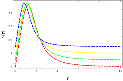
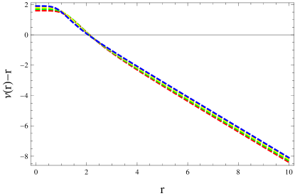
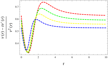
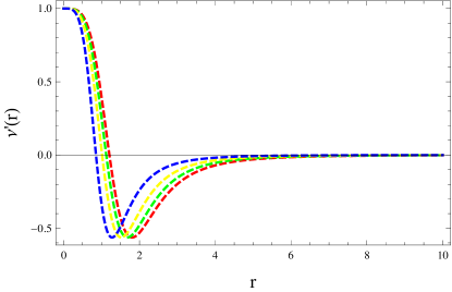
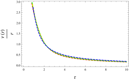
Figure 1: Behavior of Morris-Thorne conditions corresponding to developed WSF.

2.1 Embedding Diagram

Classical geometry, specifically hyperbolic and elliptic non-Euclidean geometry provides the foundation for embedding theorems. A pseudo-sphere or an ordinary sphere can be visualized within Euclidean three-space as these geometries have intrinsic curvature. The development of embedding theorems has been greatly influenced by Campbell’s theorem in the framework of general relativity (GR) [65]. The origin of matter can be explained by the resulting five-dimensional theory. In this five-dimensional framework, the vacuum field equations yield the familiar Einstein field equations supplemented with matter, leading to induced-matter theory [66]. The incorporation of an additional dimension serves the purpose of unification which greatly enhance our understanding of physics in four dimensions. Moreover, the extra dimension can be either timelike or spacelike. Consequently, the resolution of particle-wave duality is achievable through the utilization of five-dimensional dynamics, which exhibits two distinct modes based on the nature of the additional dimensions such as spacelike or timelike [67]. Thus, the theory of relativity in five dimensions leads to unification of GR and quantum field theory. The aforementioned analysis validates the effectiveness of the mathematical model known as embedding theory, based on Campbell’s theorem. However, prior to employing this framework for wormhole (WH) geometry, it is crucial to introduce a refinement in this framework.

The induced-matter theory is a theoretical framework that extends the concept of the Kaluza-Klein theory of gravity. It proposes a way to incorporate matter into the theory that embeds four-dimensional spacetime in a five-dimensional manifold, which is Ricci flat [68]. This embedding process requires only one extra dimension. In the context of embedding classes, one can embed $n$-dimensional manifold into $(n+m)$-dimensional manifold. For example, the interior Schwarzschild solution and the Friedmann universe belong to class-I, while the exterior Schwarzschild solution falls into class-II. Based on the similarities between WH spacetime and the exterior Schwarzschild solution, it is assumed that WH spacetime also belongs to class-II. Consequently, it can be embedded in a six-dimensional flat spacetime. However, it is noteworthy that a line element of class-II can be reduced to a line element of class-I. This implies that the mathematical description of WH spacetime can be transformed into a form that belongs to embedding class-I. The mathematical model proposed by the induced-matter theory has proven to be highly useful in the study of cosmic objects, likely providing insights and explanations for various phenomena and properties observed in the universe [69]-[75].

To extract useful information from WH geometry, we use embedding diagram. It is an important tool for visualizing and understanding the geometry of WHs and spacetime, in general. It allows us to represent higher-dimensional curved spacetime in a lower-dimensional Euclidean space. For a WH, a hypothetical tunnel connecting two separate regions of spacetime, an embedding diagram can help us to visualize the curvature and topology of the WH. By representing the WH in a lower-dimensional space such as a two-dimensional plane, we can gain insights into its shape and properties. To construct an embedding diagram for a WH, we consider a spherically symmetric spacetime. This means that the geometry of the WH remains the same along spherical slices. In particular, we can focus on an equator slice where the angular coordinate $\theta$ is fixed at $\frac{\pi}{2}$. By choosing a constant time slice ($t=$ constant), we can examine the spatial geometry of the WH independent of time. In this equatorial slice, we can plot the spatial geometry of the WH in the embedding diagram. The embedding diagram will typically be a two-dimensional representation, where one axis represents the radial distance from the WH center and the other axis represents some other relevant coordinate or property. It is important to note that an embedding diagram provides a simplified visualization and is not a complete representation of the WH spacetime. Nevertheless, it can be a helpful tool for gaining insights into the geometric properties of WHs and understanding the effects of gravity in our universe.

Using these assumptions in Eq.(5), we have

$$ds^{2}=dr^{2}\left(\frac{r}{r-\nu}\right)+r^{2}d\phi^{2}.$$ (13)

This embedding equation in cylindrical coordinates $(r,h,\phi)$ is written as

$$ds^{2}=dr^{2}+dh^{2}+r^{2}d\phi^{2}=dr^{2}\left[1+(\frac{dh}{dr})^{2}\right]+r^{2}d\phi^{2}.$$ (14)

Comparison of Eqs.(14) and (15) gives

$$\frac{dh}{dr}=\pm\left(\frac{r}{\nu}-1\right)^{\frac{-1}{2}}.$$ (15)

The embedding diagram for the upper universe ($h>0$) and the lower universe ($h<0$) using a slice $t=$ constant and $\theta=\frac{\pi}{2}$ corresponding to radial coordinate is shown in Figures 2 and 3, respectively. Moreover, Eq.(15) indicates that the embedded surface is vertical at the WH throat, i.e., $\frac{dh}{dr}\rightarrow\infty$. We also examine that the space is asymptotically flat away from the throat because $\frac{dh}{dr}$ tends to zero as $r$ tends to infinity. One can visualize the upper universe for $h>0$ and the lower universe $h<0$ in Figures 2 and 3, respectively. One can consider a $2\pi$ rotation around the $h$-axis for the full visualization of the WH surface.

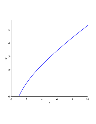
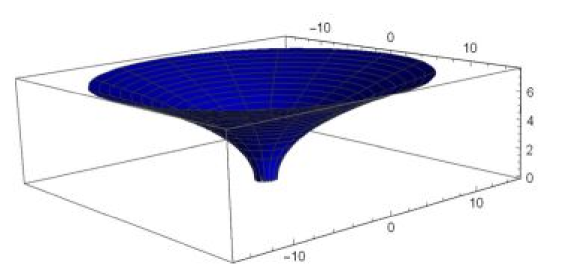
Figure 2: Graph of embedding diagram for $h(r)>0$ (upper universe) with slice $t=$ constant and $\theta=\frac{\pi}{2}$.

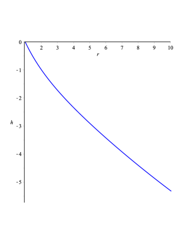
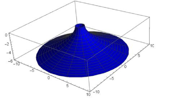
Figure 3: Graph of embedding diagram for $h(r)<0$ (lower universe) with slice $t=$ constant and $\theta=\frac{\pi}{2}$.

3 Basic Formalism of $f(\mathcal{G})$ Gravity

The corresponding action is defined as [43]

$$\mathcal{I}=\frac{1}{2\kappa}\int\mathfrak{R}{\sqrt{-\mathrm{g}}}d^{4}x+\frac{1}{2\kappa}\int f(\mathcal{G}){\sqrt{-\mathrm{g}}}d^{4}x+\int(\mathcal{L}_{m}+\mathcal{L}_{e})\sqrt{-\mathrm{g}}d^{4}x,$$ (16)

where the matter-lagrangian and determinant of the line element are represented by $\mathcal{L}_{m}$ and $\mathrm{g}$, respectively. The electromagnetic-lagrangian is expressed as

$$\mathcal{L}_{e}=\epsilon\mathcal{F}_{\alpha\beta}\mathcal{F}^{\alpha\beta},\quad\mathcal{F}_{\alpha\beta}=\varphi_{\beta,\alpha}-\varphi_{\alpha,\beta},$$

where $\epsilon$ is an arbitrary constant and $\varphi_{\alpha}$ is the four-potential. By varying Eq.(16) corresponding to metric tensor, we obtain

$$\mathfrak{R}_{\alpha\beta}-\frac{1}{2}\mathrm{g}_{\alpha\beta}\mathfrak{R} = \kappa(\mathcal{T}_{\alpha\beta}+\mathcal{E}_{\alpha\beta})-8\big{(}\mathfrak{R}_{\alpha\lambda\beta\delta}+\mathfrak{R}_{\lambda\beta}\mathrm{g}_{\delta\alpha}-\mathfrak{R}_{\lambda\delta}\mathrm{g}_{\alpha\beta}-\mathfrak{R}_{\alpha\beta}\mathrm{g}_{\lambda\delta}$$ (17)

$$+ \mathfrak{R}_{\alpha\delta}\mathrm{g}_{\beta\lambda}+\frac{1}{2}\mathfrak{R}(g_{\alpha\beta}\mathrm{g}_{\lambda\delta}-\mathrm{g}_{\alpha\delta}\mathrm{g}_{\beta\lambda})\big{)}\nabla^{\lambda}\nabla^{\delta}+\big{(}4\mathrm{g}_{\alpha\beta}\mathfrak{R}^{\lambda\delta}\nabla_{\lambda}\nabla_{\delta}$$

$$+ 2\mathfrak{R}\nabla_{\alpha}\nabla_{\beta}-2g_{\alpha\beta}\mathfrak{R}\nabla_{\alpha}\nabla^{\alpha}-4\mathfrak{R}^{\lambda}_{\alpha}\nabla_{\beta}\nabla_{\lambda}-4\mathfrak{R}^{\lambda}_{\beta}\nabla_{\alpha}\nabla_{\lambda}$$

$$- 4\mathfrak{R}_{\alpha\lambda\beta\delta}\nabla^{\lambda}\nabla^{\delta}\big{)}f_{\mathcal{G}}.$$

Here, $f\equiv f(\mathcal{G})$ and $f_{\mathcal{G}}=\frac{\partial f}{\partial\mathcal{G}}$. The stress-energy tensor of electric field is expressed as

$$\mathcal{E}_{\alpha\beta}=\frac{1}{4\pi}\left[\frac{\mathcal{F}^{\lambda\delta}\mathcal{F}_{\lambda\delta}\mathrm{g}_{\alpha\beta}}{4}-\mathcal{F}^{\lambda}_{\alpha}\mathcal{F}_{\beta\lambda}\right].$$ (18)

We assume anisotropic matter distribution as

$$\mathcal{T}_{\alpha\beta}=\mathcal{V}_{\alpha}\mathcal{V}_{\beta}(\rho+p_{t})-p_{t}g_{\alpha\beta}+\mathcal{U}_{\alpha}\mathcal{U}_{\beta}(p_{r}-p_{t}),$$ (19)

where $\rho$ represents the energy density, $\mathcal{V}_{\alpha}$ is the four-velocity, $\mathcal{U}_{\alpha}$ defines four-vector, $p_{r}$ denotes the radial pressure and $p_{t}$ is tangential pressure.

The Maxwell field equations are defined as

$$\mathcal{F}_{\alpha\beta;\lambda}=0,\quad F^{\alpha\beta}_{;\beta}=4\pi\mathcal{J}^{\alpha},$$ (20)

where four-current is defined by $\mathcal{J}^{\alpha}$. In comoving coordinates, $\varphi^{\alpha}$ and $\mathcal{J}^{\alpha}$ fulfill the following relations

$$\varphi^{\alpha}=\phi(r)\delta^{\alpha}_{0},\quad\mathcal{J}^{\alpha}=\sigma\mathcal{V}^{\alpha},$$ (21)

where $\sigma=\sigma(r)$ is the charge density. The resulting electromagnetic field equation is

$$\varphi^{\prime\prime}+\bigg{(}\frac{2}{r}-\frac{a^{\prime}}{2}-\frac{b^{\prime}}{2}\bigg{)}\varphi^{\prime}=4\pi\sigma e^{\frac{a}{2}+b}.$$ (22)

Integrating this equation, we get

$$\varphi^{\prime}=\frac{qe^{\frac{a+b}{2}}}{r^{2}},\quad q(r)=4\pi\int_{0}^{r}\sigma r^{2}e^{\frac{b}{2}}dr,\quad E=\frac{q}{4\pi r^{2}},$$ (23)

where $E$ is the charge intensity and $q$ represents the charge inside the interior of WH. Using Eqs.(1) and (17), we obtain the field equations of charged anisotropic spherical system as

$$\rho = \frac{e^{-2b}}{2r^{2}}\bigg{[}-2e^{b}+2e^{2b}-e^{2b}r^{2}f+e^{2b}r^{2}\mathcal{G}f_{\mathcal{G}}+2b^{\prime}(re^{b}-2(e^{b}-3)\mathcal{G}^{\prime}f_{\mathcal{G}\mathcal{G}})$$

$$- 8(\mathcal{G}^{\prime\prime}f_{\mathcal{G}\mathcal{G}}+\mathcal{G}^{\prime 2}f_{\mathcal{G}\mathcal{G}\mathcal{G}})(1-e^{b})-\frac{2q^{2}r^{2}}{8\pi r^{4}e^{-2b}}\bigg{]},$$

$$p_{r} = \frac{e^{-2b}}{2r^{2}}\bigg{[}e^{b}(2+e^{b}(r^{2}f-2))-e^{2b}r^{2}\mathcal{G}f_{\mathcal{G}}+2a^{\prime}(re^{b}-2(e^{b}-3)\mathcal{G}^{\prime}f_{\mathcal{G}\mathcal{G}})$$

$$+ \frac{2q^{2}r^{2}}{8\pi r^{4}e^{-2b}}\bigg{]},$$

$$p_{t} = \frac{e^{-2b}}{4r}\bigg{[}-2e^{2b}r\mathcal{G}f_{\mathcal{G}}+a^{\prime 2}(re^{b}+4\mathcal{G}^{\prime}f_{\mathcal{G}\mathcal{G}})+2(e^{2b}rf-b^{\prime}e^{b}+(e^{b}r+4\mathcal{G}^{\prime}f_{\mathcal{G}\mathcal{G}})a^{\prime\prime})$$

$$+ a^{\prime}\big{\{}-b^{\prime}(e^{b}r+12\mathcal{G}^{\prime}f_{\mathcal{G}\mathcal{G}})+2(e^{b}+4(\mathcal{G}^{\prime\prime}f_{\mathcal{G}\mathcal{G}}+\mathcal{G}^{\prime 2}f_{\mathcal{G}\mathcal{G}\mathcal{G}}))\big{\}}-\frac{2q^{2}r^{2}}{8\pi r^{4}e^{-2b}}\bigg{]}.$$

where

$$\mathcal{G} = -\frac{2}{r^{2}e^{2b}}\big{[}(e^{b}-3)a^{\prime}b^{\prime}-(e^{b}-1)(2a^{\prime\prime}+a^{\prime 2})\big{]},$$

$$\mathcal{G}^{\prime} = \frac{2}{r^{3}e^{2b}}\bigg{[}2(e^{b}-1)a^{\prime 2}+(6-e^{b})ra^{\prime}b^{\prime 2}+2(e^{b}-1)(2a^{\prime\prime}-a^{\prime\prime\prime})+ra^{\prime}(e^{b}-3)b^{\prime\prime}$$

$$- 2(e^{b}-1)a^{\prime\prime}+b^{\prime}\{2(3-e^{b})a^{\prime}+(3e^{b}-7)ra^{\prime\prime}+(e^{b}-2)ra^{\prime 2}\}\bigg{]},$$

$$\mathcal{G}^{\prime\prime} = \frac{2}{r^{4}e^{2b}}\bigg{[}a^{\prime 2}{6-6e^{b}+(e^{b}-2)r^{2}b^{\prime\prime}}+(e^{b}-12)r^{2}a^{\prime}b^{\prime 3}-2\bigg{\{}a^{\prime\prime}\big{\{}6(e^{b}-1)$$

$$- (2e^{b}-5)r^{2}b^{\prime\prime}+(e^{b}-1)r^{2}a^{\prime\prime 2}+(e^{b}-1)r(2a^{\prime\prime\prime}-4a^{\prime\prime\prime})\big{\}}\bigg{\}}+b^{\prime}\bigg{\{}a^{\prime}(6(e^{b}-3)$$

$$+ 4(e^{b}-2)r^{2}a^{\prime\prime}-3(e^{b}-6)r^{2}b^{\prime\prime})-4(e^{b}-2)ra^{\prime 2}+r(a^{\prime\prime\prime}(5e^{b}-11)r$$

$$- 4(3e^{b}-7)a^{\prime\prime})\bigg{\}}-rb^{\prime 2}{4(e^{b}-5)ra^{\prime\prime}-(e^{b}-6)a^{\prime}+(e^{b}-4)ra^{\prime 2}}+ra^{\prime}\big{\{}8a^{\prime\prime}$$

$$\times (e^{b}-1)-4(e^{b}-3)b^{\prime\prime}+r\big{(}(e^{b}-3)b^{\prime\prime\prime}-2a^{\prime\prime\prime}(e^{b}-1)\big{)}\big{\}}\bigg{]}.$$

4 Energy Conditions

There are certain constraints named as energy conditions that must be imposed on the matter to examine the presence of some viable cosmic structures. These constraints are a set of inequalities that impose limitations on the energy-momentum tensor which governs the behavior of matter and energy in the presence of gravity. The stress-energy tensor describes the distribution of energy, momentum and stress in a given region of spacetime. There are several energy conditions, each of which places different constraints on the stress-energy tensor as

• Null energy constraint
  
  This condition states that the energy density measured by any null (light-like) observer is non-negative. The addition of energy density and pressure components must be non-negative according to this condition. Mathematically, this can be defined as

  $$p_{r}+\rho\geq 0,\quad p_{t}+\rho\geq 0.$$

• Dominant energy constraint
  
  This determines that the energy flux measured by any observer cannot exceed the energy density. Mathematically, it is expressed as

  $$\rho-p_{r}\geq 0,\quad\rho-p_{t}\geq 0.$$

• Weak energy constraint
  
  The weak energy condition states that the energy density measured by any observer is non-negative. Also, the sum of energy density and pressure components are non-negative. Mathematically, this means that

  $$p_{r}+\rho\geq 0,\quad p_{t}+\rho\geq 0,\quad\rho\geq 0.$$

• Strong energy constraint
  
  This energy condition is a stronger version of the weak energy constraint and states that not only is the energy density non-negative, but the addition of $\rho$ and pressure components is also non-negative, defined as

  $$p_{r}+\rho\geq 0,\quad p_{t}+\rho\geq 0,\quad p_{r}+2p_{t}+\rho\geq 0.$$

These energy bounds are significant in determining the presence of cosmic structures. They also have implications for the behavior of exotic matter and the existence of traversable WH geometry and other hypothetical objects in spacetime. The viable WH structure must violate these conditions.

The graphical behavior of energy conditions for $f(\mathcal{G})=0$ is given in Figure 4. In the upper panel, the behavior of $\rho+p_{t}$ is positive but negative behavior of $\rho+p_{r}$ shows that the null energy condition is violated. Furthermore, the graphs in the middle part manifest that the dominant energy condition is violated as the behavior of $\rho-p_{t}$ is negative. The components $\rho$ and $\rho+p_{r}+2p_{t}$ also exhibit negative trends, indicating the violation of strong and weak energy conditions, respectively. Thus, a viable traversable WH structure can be obtained in this gravity model.

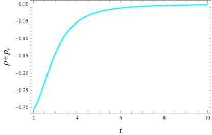
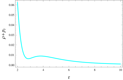
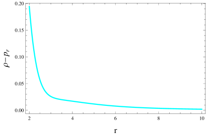
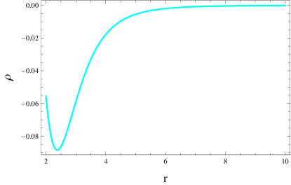
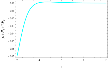
Figure 4: Plots of energy conditions for $f(\mathcal{G})=0$.

4.1 Viable $f(\mathcal{G})$ Models

Here, we examine how various models of $f(\mathcal{G})$ affect the geometry of WH. The outcomes of our research may uncover concealed cosmological findings on both theoretical and astrophysical levels. Some notable outcomes indicate the existence of additional correction terms from modified gravitational theories, which could yield some motivational results. These correction terms have a significant influence on the collapse rate and the presence of viable geometry as compared to GR. Hence, it is valuable to explore alternative theories such as $f(\mathcal{G})$ to determine the presence of hypothetical objects. This could serve as a mathematical tool for examining various obscure features of gravitational dynamics on a large scale. In the next subsections, we investigate three distinct $f(\mathcal{G})$ models as

4.2 Model l

We first consider the power-law model with the logarithmic correction term as [76]

$$f(\mathcal{G})=\gamma_{1}\mathcal{G}^{m_{1}}+\xi_{1}\mathcal{G}\ln(\mathcal{G}),$$ (24)

where $\gamma_{1}$, $\xi_{1}$ and $m_{1}$ are arbitrary constants. Since this model allows extra degrees of freedom in the field equations, therefore, it could provide observationally well-consistent cosmic results. The resulting equations of motion are

$$\rho = \frac{e^{-2b}}{2r^{2}}\bigg{[}-2e^{b}+2e^{2b}-e^{2b}r^{2}(\gamma_{1}\mathcal{G}^{m_{1}}+\xi_{1}\mathcal{G}\ln(\mathcal{G}))+e^{2b}r^{2}\mathcal{G}(\gamma_{1}\mathcal{G}^{m_{1}-1}m_{1}$$

$$+ \xi_{1}\ln(\mathcal{G})+\xi_{1})+2b^{\prime}\big{\{}re^{b}-2(e^{b}-3)\big{\{}\gamma_{1}m_{1}(m_{1}-1)\mathcal{G}^{m_{1}-2}\mathcal{G}^{\prime}+\xi_{1}\mathcal{G}^{-1}\mathcal{G}^{\prime}\big{\}}\big{\}}$$

$$- 8(1-e^{b})\bigg{\{}\mathcal{G}^{\prime\prime}\big{\{}\gamma_{1}m_{1}(m_{1}-1)\mathcal{G}^{m_{1}-2}+\xi_{1}\mathcal{G}^{-1}\big{\}}+\mathcal{G}^{\prime 2}\big{\{}\gamma_{1}(m_{1}-1)(m_{1}-2)$$

$$\times m_{1}\mathcal{G}^{m_{1}-3}-\xi_{1}\mathcal{G}^{-2}\big{\}}\bigg{\}}-\frac{2q^{2}r^{2}}{8\pi r^{4}e^{-2b}}\bigg{]},$$

$$p_{r} = \frac{e^{-2b}}{2r^{2}}\bigg{[}e^{b}(2+e^{b}(r^{2}(\gamma_{1}\mathcal{G}^{m_{1}}+\xi_{1}\mathcal{G}\ln(\mathcal{G}))-2))-e^{2b}r^{2}\mathcal{G}(\gamma_{1}\mathcal{G}^{m_{1}-1}m_{1}+\xi_{1}\ln(\mathcal{G})$$

$$+ \xi_{1})+2a^{\prime}\big{\{}re^{b}-2(e^{b}-3)\big{\{}\gamma_{1}m_{1}(m_{1}-1)\mathcal{G}^{m_{1}-2}\mathcal{G}^{\prime}+\xi_{1}\mathcal{G}^{-1}\mathcal{G}^{\prime}\big{\}}\big{\}}+\frac{2q^{2}r^{2}}{8\pi r^{4}e^{-2b}}\bigg{]},$$

$$p_{t} = \frac{e^{-2b}}{4r}\bigg{[}-2e^{2b}r\mathcal{G}(\gamma_{1}\mathcal{G}^{m_{1}-1}m_{1}+\xi_{1}\ln(\mathcal{G})+\xi_{1})+a^{\prime 2}\big{\{}re^{b}+4\big{\{}\gamma_{1}m_{1}(m_{1}-1)$$

$$\times \mathcal{G}^{n-2}\mathcal{G}^{\prime}+\xi_{1}\mathcal{G}^{-1}\mathcal{G}^{\prime}\big{\}}\big{\}}+2\bigg{\{}e^{2b}r(\gamma_{1}\mathcal{G}^{m_{1}}+\xi_{1}\mathcal{G}\ln(\mathcal{G}))-b^{\prime}e^{b}+\big{\{}e^{b}r+4\big{\{}\gamma_{1}m_{1}$$

$$\times (m_{1}-1)\mathcal{G}^{m_{1}-2}\mathcal{G}^{\prime}+\xi_{1}\mathcal{G}^{-1}\mathcal{G}^{\prime}\big{\}}\big{\}}a^{\prime\prime}\bigg{\}}+a^{\prime}\bigg{[}-b^{\prime}(e^{b}r+12\big{\{}\gamma_{1}m_{1}(m_{1}-1)$$

$$\times \mathcal{G}^{n-2}\mathcal{G}^{\prime}+\xi_{1}\mathcal{G}^{-1}\mathcal{G}^{\prime}\big{\}})+2\bigg{\{}e^{b}+4\big{\{}\mathcal{G}^{\prime\prime}\big{\{}\gamma_{1}m_{1}(m_{1}-1)\mathcal{G}^{m_{1}-2}+\xi_{1}\mathcal{G}^{-1}\big{\}}$$

$$+ \mathcal{G}^{\prime 2}\big{\{}\gamma_{1}m_{1}(m_{1}-1)(m_{1}-2)\mathcal{G}^{m_{1}-3}-\xi_{1}\mathcal{G}^{-2}\big{\}}\big{\}}\bigg{\}}\bigg{]}-\frac{2q^{2}r^{2}}{8\pi r^{4}e^{-2b}}\bigg{]}.$$

We consider radial dependent form of the charge as $q(r)=\chi r^{3}$ [77], where $\chi$ is an arbitrary constant. We choose $\chi=0.0001$ for our convenience in all the graphs. Figures 5 and 6 depict the graphical representation of energy bounds for different values of model parameters. The behavior of energy bounds for positive values of $\gamma_{1}$, $\xi_{1}$ and $m_{1}$ is analyzed in Figure 5. The plots in the upper panel indicate that the behavior of $\rho+p_{r}$ and $\rho+p_{t}$ is negative which implies that the null energy condition is violated. The middle part shows that the dominant energy constraint is violated due to the negative behavior of $\rho-p_{r}$ and $\rho-p_{t}$. The behavior of energy density is also negative which violates the weak energy condition. Although $\rho+p_{r}+2p_{t}$ is positive near the center of the star but becomes negative at the surface boundary, leading to a violation of the strong energy condition.

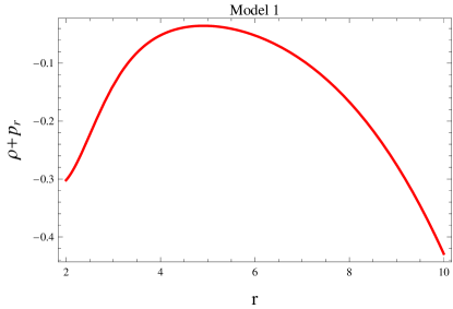
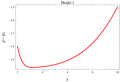
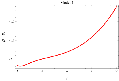
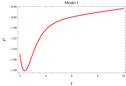
Figure 5: Plots of energy conditions for $\gamma_{1}=2$, $\xi_{1}=0.0003$, $m_{1}=0.0005$.

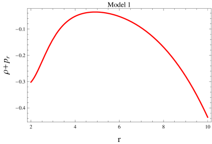
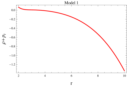
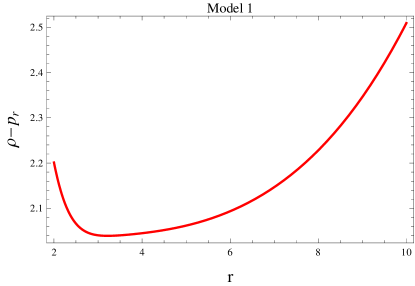
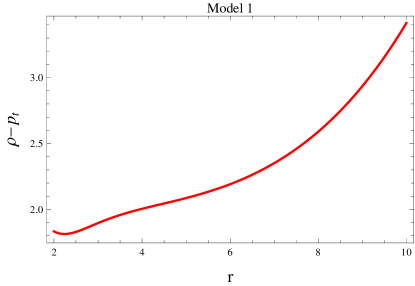
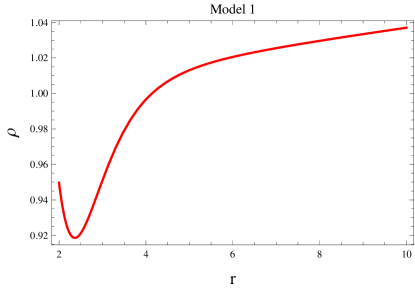
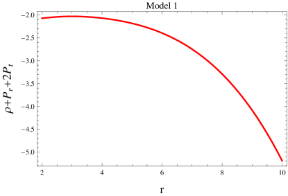
Figure 6: Plots of energy conditions for $\gamma_{1}=-2$, $\xi_{1}=-0.0003$, $m_{1}=-0.0005$.

Figure 6 manifests the behavior of energy conditions for positive values of $\gamma_{1}$, $\xi_{1}$ and $m_{1}$. The upper panel violates the null energy condition because $\rho+p_{r}$ and $\rho+p_{t}$ show negative behavior. However, the positive behavior of $\rho-p_{r}$ and $\rho-p_{t}$ satisfies the dominant energy condition. We also note that the $\rho$ is positive but the negative behavior of $\rho+p_{r}$ and $\rho+p_{t}$ violates the weak energy condition. The representation of $\rho+p_{r}+2p_{t}$ exhibits negative trend as shown in the below panel which implies that the strong energy condition is also violated. These graphs manifest that fluid parameters violate the energy conditions especially the violation of the null energy condition for both positive as well as negative values of $\gamma_{1}$, $\xi_{1}$ and $m_{1}$ provide viable traversable WH structure in $f(\mathcal{G})$ gravity model. However, we have also checked that the energy bounds violate for alternative parametric values.

4.3 Model 2

Here, we use another model as [78]

$$f(\mathcal{G})=\gamma_{2}\mathcal{G}^{m_{2}}(\xi_{2}\mathcal{G}^{n}+1),$$

where $\gamma_{2}$, $\xi_{2}$ and $n$ are arbitrary constant and $m_{2}>0$. This model is extremely useful for the dealing with finite time future singularities. The corresponding field equations are

$$\rho = \frac{e^{-2b}}{2r^{2}}\bigg{[}-2e^{b}+2e^{2b}-e^{2b}r^{2}(\gamma_{2}\mathcal{G}^{m_{2}}(\xi_{2}\mathcal{G}^{n}+1))+e^{2b}r^{2}\mathcal{G}\big{\{}\gamma_{2}\xi_{2}(m_{2}+n)$$

$$\times \mathcal{G}^{m_{2}+n-1}+\gamma_{2}m_{2}\mathcal{G}^{m_{2}-1}\big{\}}+2b^{\prime}\bigg{\{}re^{b}-2(e^{b}-3)\big{\{}(m_{2}+n)(m_{2}+n-1)$$

$$\times \gamma_{2}\xi_{2}\mathcal{G}^{\prime}\mathcal{G}^{m_{2}+n-2}+\gamma_{2}m_{2}(m_{2}-1)\mathcal{G}^{\prime}\mathcal{G}^{m_{2}-2}\big{\}}\bigg{\}}-8(1-e^{b})\bigg{[}(m_{2}+n-1)$$

$$\times \gamma_{2}\xi_{2}(m_{2}+n)\mathcal{G}^{\prime\prime}\mathcal{G}^{m_{2}+n-2}+\gamma_{2}m_{2}(m_{2}-1)\mathcal{G}^{\prime\prime}\mathcal{G}^{m_{2}-2}+\gamma_{2}\xi_{2}(m_{2}+n-1)$$

$$\times (m_{2}+n)(m_{2}+n-2)\mathcal{G}^{\prime 2}\mathcal{G}^{m_{2}+n-3}+\gamma_{2}m_{2}(m_{2}-1)(m_{2}-2)\mathcal{G}^{\prime 2}\mathcal{G}^{m_{2}-3}\bigg{]}$$

$$- \frac{2q^{2}r^{2}}{8\pi r^{4}e^{-2b}}\bigg{]},$$

$$p_{r} = \frac{e^{-2b}}{2r^{2}}\bigg{[}e^{b}(2+e^{b}(r^{2}(\gamma_{2}\mathcal{G}^{m_{2}}(\xi_{2}\mathcal{G}^{n}+1))-2))-e^{2b}r^{2}\mathcal{G}\big{\{}\gamma_{2}\xi_{2}\mathcal{G}^{m_{2}+n-1}$$

$$\times (m_{2}+n)+\gamma_{2}m_{2}\mathcal{G}^{m_{2}-1}\big{\}}+2a^{\prime}\bigg{\{}re^{b}-2(e^{b}-3)\big{\{}(m_{2}+n)(m_{2}+n-1)$$

$$\times \gamma_{2}\xi_{2}\mathcal{G}^{\prime}\mathcal{G}^{m_{2}+n-2}+\gamma_{2}m_{2}(m_{2}-1)\mathcal{G}^{\prime}\mathcal{G}^{m_{2}-2}\big{\}}\bigg{\}}+\frac{2q^{2}r^{2}}{8\pi r^{4}e^{-2b}}\bigg{]},$$

$$p_{t} = \frac{e^{-2b}}{4r}\bigg{[}-2e^{2b}r\mathcal{G}f_{\mathcal{G}}+a^{\prime 2}(re^{b}+4\mathcal{G}^{\prime}f_{\mathcal{G}\mathcal{G}})+2\bigg{\{}e^{2b}r(\gamma_{2}\mathcal{G}^{m_{2}}(\xi_{2}\mathcal{G}^{n}+1))$$

$$- b^{\prime}e^{b}+\big{\{}e^{b}r+4\big{\{}\gamma_{2}\xi_{2}(m_{2}+n)(m_{2}+n-1)\mathcal{G}^{\prime}\mathcal{G}^{m_{2}+n-2}+\gamma_{2}m_{2}(m_{2}-1)$$

$$\times \mathcal{G}^{\prime}\mathcal{G}^{m_{2}-2}\big{\}}\big{\}}a^{\prime\prime}\bigg{\}}+a^{\prime}\bigg{[}-b^{\prime}\big{\{}e^{b}r+12\big{\{}\gamma_{2}\xi_{2}(m_{2}+n)(m_{2}+n-1)\mathcal{G}^{\prime}\mathcal{G}^{m_{2}+n-2}$$

$$+ \gamma_{2}m_{2}(m_{2}-1)\mathcal{G}^{\prime}\mathcal{G}^{m_{2}-2}\big{\}}\big{\}}+2\bigg{\{}e^{b}+4\big{\{}\gamma_{2}\xi_{2}(m_{2}+n)(m_{2}+n-1)\mathcal{G}^{\prime\prime}\mathcal{G}^{m_{2}+n-2}$$

$$+ \gamma_{2}m_{2}(m_{2}-1)\mathcal{G}^{\prime\prime}\mathcal{G}^{m_{2}-2}+\gamma_{2}\xi_{2}(m_{2}+n)(m_{2}+n-1)(m_{2}+n-2)\mathcal{G}^{\prime 2}\mathcal{G}^{m_{2}+n-3}$$

$$+ \gamma_{2}m_{2}(m_{2}-1)(m_{2}-2)\mathcal{G}^{\prime 2}\mathcal{G}^{m_{2}-3}\big{\}}\bigg{\}}\bigg{]}-\frac{2q^{2}r^{2}}{8\pi r^{4}e^{-2b}}\bigg{]}.$$

We consider $m_{2}=0.0005$ for our convenience in the graphical analysis. We investigate the viable characteristics of WH by analyzing the above equations. Figure 7 determines the behavior of energy bounds for positive values of $\gamma_{2}$, $\xi_{2}$ and $n$. In the upper panel, the negative behavior of $\rho+p_{r}$ and $\rho+p_{t}$ show that the null energy condition is violated. Furthermore, the graphs in the middle part manifest that the dominant energy condition is satisfied as the behavior of $\rho-p_{r}$ and $\rho-p_{t}$ is positive. The components $\rho$ and $\rho+p_{r}+2p_{t}$ also exhibit negative trends, indicating the violation of strong and weak energy conditions, respectively. Figure 8 represents the energy conditions for negative values of the model parameters. These graphs show that the fluid parameters satisfy the energy conditions, i.e., the behavior of matter components $(\rho,\rho\pm p_{r},\rho\pm p_{t})$ is positive for negative values of $\gamma_{2}$, $\xi_{2}$ and $n$ which yields non-traversable WH structure. Hence, in this gravity model, a viable traversable WH structure can be obtained for positive values of the model parameter.

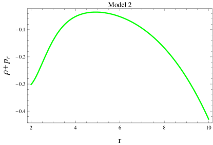
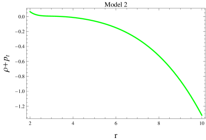
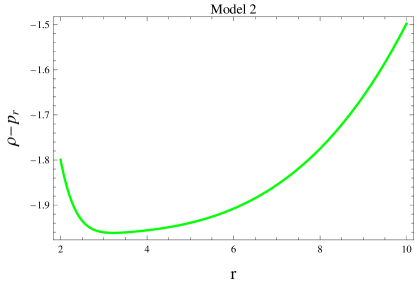
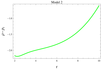
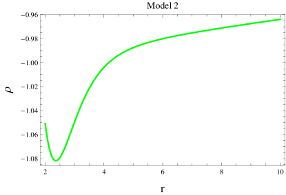
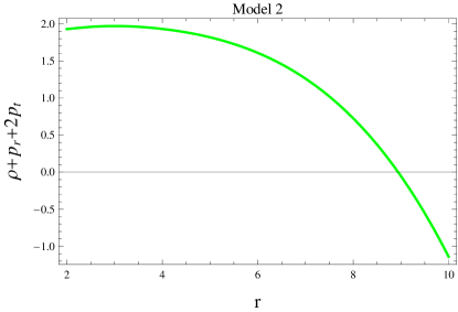
Figure 7: Plots of energy conditions for $\gamma_{2}=2$, $\xi_{2}=0.0003$ and $n=0.001$.

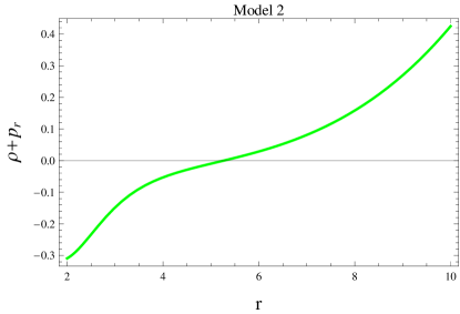
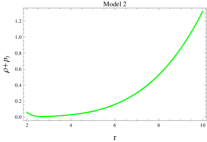
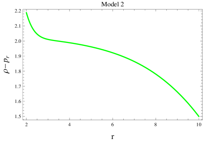
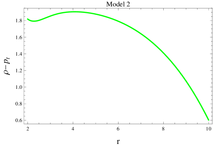
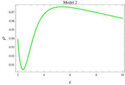
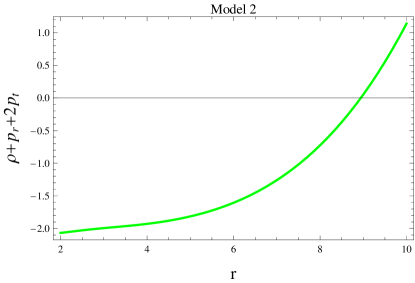
Figure 8: Plots of energy conditions for $\gamma_{2}=-2$, $\xi_{2}=-0.0003$ and $n=-0.001$.

4.4 Model 3

Finally, we consider the following viable model as

$$f(\mathcal{G})=\frac{\gamma_{3}\mathcal{G}^{m_{3}}+\xi_{3}}{\gamma_{4}\mathcal{G}^{m_{3}}+\xi_{4}}.$$

Here $\gamma_{3}$, $\gamma_{4}$, $\xi_{3}$ and $\xi_{4}$ are arbitrary constants with $m_{3}>0$. The corresponding field equations are

$$\rho = \frac{e^{-2b}}{2r^{2}}\bigg{[}-2e^{b}+2e^{2b}-e^{2b}r^{2}(\gamma_{3}\mathcal{G}^{m_{3}}+\xi_{3})(\gamma_{4}\mathcal{G}^{m_{3}}+\xi_{4})^{-1}+\frac{e^{2b}r^{2}}{(\gamma_{4}\mathcal{G}^{m_{3}}+\xi_{4})^{2}}$$

$$\times \big{\{}(\gamma_{4}\mathcal{G}^{m_{3}}+\xi_{4})(\gamma_{3}m_{3}\mathcal{G}^{m_{3}-1})+(\gamma_{3}\mathcal{G}^{m_{3}}+\xi_{3})(\gamma_{4}m_{3}\mathcal{G}^{m_{3}-1})\big{\}}+2b^{\prime}\bigg{[}re^{b}$$

$$- \frac{2(e^{b}-3)\mathcal{G}^{\prime}}{(\gamma_{4}\mathcal{G}^{m_{3}}+\xi_{4})^{3}}\bigg{[}m_{3}\bigg{\{}(\mathcal{G}^{2m_{3}-2}\xi_{3}\gamma_{4}^{2}m_{3}-\mathcal{G}^{2m_{3}-2}\xi_{4}\gamma_{3}\gamma_{4}m_{3}+\mathcal{G}^{2m_{3}-2}\xi_{3}\gamma_{4}^{2}-\xi_{4}\gamma_{3}$$

$$\times \gamma_{4}\mathcal{G}^{2m_{3}-2}-\mathcal{G}^{m_{3}-2}\xi_{3}\xi_{4}\gamma_{4}m_{3}+\mathcal{G}^{m_{3}-2}\xi_{4}^{2}\gamma_{3}m_{3}+\mathcal{G}^{m_{3}-2}\xi_{3}\xi_{4}\gamma_{4}-\mathcal{G}^{m_{3}-2}\xi_{4}^{2}\gamma_{3}\bigg{\}}\bigg{]}\bigg{]}$$

$$- 8\mathcal{A}(1-e^{b})-\frac{2q^{2}r^{2}}{8\pi r^{4}e^{-2b}}\bigg{]},$$

$$p_{r} = \frac{e^{-2b}}{2r^{2}}\bigg{[}e^{b}(2+e^{b}\big{\{}(r^{2}(\gamma_{3}\mathcal{G}^{m_{3}}+\xi_{3})(\gamma_{4}\mathcal{G}^{m_{3}}+\xi_{4})^{-1}-2)\big{\}}-\frac{e^{2b}r^{2}\mathcal{G}}{(\gamma_{4}\mathcal{G}^{m_{3}}+\xi_{4})^{2}}$$

$$\times \big{\{}(\gamma_{4}\mathcal{G}^{m_{3}}+\xi_{4})(\gamma_{3}m_{3}\mathcal{G}^{m_{3}-1})+(\gamma_{3}\mathcal{G}^{m_{3}}+\xi_{3})(\gamma_{4}m_{3}\mathcal{G}^{m_{3}-1})\big{\}}+2a^{\prime}\bigg{\{}re^{b}$$

$$- \frac{2(e^{b}-3)\mathcal{G}^{\prime}}{(\gamma_{4}\mathcal{G}^{m_{3}}+\xi_{4})^{2}}\big{\{}(\gamma_{4}\mathcal{G}^{m_{3}}+\xi_{4})(\gamma_{3}m_{3}\mathcal{G}^{m_{3}-1})+(\gamma_{3}\mathcal{G}^{m_{3}}+\xi_{3})(\gamma_{4}m_{3}\mathcal{G}^{m_{3}-1})\big{\}}\bigg{\}}$$

$$+ \frac{2q^{2}r^{2}}{8\pi r^{4}e^{-2b}}\bigg{]},$$

$$p_{t} = \frac{e^{-2b}}{4r}\bigg{[}-\frac{2e^{2b}r\mathcal{G}}{(\gamma_{4}\mathcal{G}^{m_{3}}+\xi_{4})^{2}}\big{\{}(\gamma_{4}\mathcal{G}^{m_{3}}+\xi_{4})(\gamma_{3}m_{3}\mathcal{G}^{m_{3}-1})+(\gamma_{4}m_{3}\mathcal{G}^{m_{3}-1})$$

$$\times (\gamma_{3}\mathcal{G}^{m_{3}}+\xi_{3})\big{\}}+a^{\prime 2}\bigg{\{}re^{b}+\frac{4\mathcal{G}^{\prime}}{(\gamma_{4}\mathcal{G}^{m_{3}}+\xi_{4})^{3}}\big{\{}m_{3}\big{\{}\mathcal{G}^{2m_{3}-2}\xi_{3}\gamma_{4}^{2}m_{3}-\xi_{4}\gamma_{3}\gamma_{4}$$

$$\times m_{3}\mathcal{G}^{2m_{3}-2}+\mathcal{G}^{2m_{3}-2}\xi_{3}\gamma_{4}^{2}-\mathcal{G}^{2m_{3}-2}b_{4}\gamma{3}\gamma_{4}-\mathcal{G}^{m_{3}-2}\xi_{3}\xi_{4}\gamma_{4}m_{3}+\mathcal{G}^{m_{3}-2}\xi_{4}^{2}\gamma_{3}m_{3}$$

$$+ \mathcal{G}^{m_{3}-2}\xi_{3}\xi_{4}\gamma_{4}-\mathcal{G}^{m_{3}-2}\xi_{4}^{2}\gamma_{3}\big{\}}\big{\}}\bigg{\}}+2\bigg{[}e^{2b}r(\gamma_{3}\mathcal{G}^{m_{3}}+\xi_{3})(\gamma_{4}\mathcal{G}^{m_{3}}+\xi_{4})^{-1}-b^{\prime}e^{b}$$

$$+ \bigg{\{}e^{b}r+\frac{4\mathcal{G}^{\prime}}{(\gamma_{4}\mathcal{G}^{m_{3}}+\xi_{4})^{3}}\big{\{}m_{3}\big{\{}\mathcal{G}^{2m_{3}-2}\xi_{3}\gamma_{4}^{2}m_{3}-\mathcal{G}^{2m_{3}-2}\xi_{4}\gamma_{3}\gamma_{4}m_{3}+\mathcal{G}^{2m_{3}-2}\xi_{3}\gamma_{4}^{2}$$

$$- \mathcal{G}^{2m_{3}-2}\xi_{4}\gamma_{3}\gamma_{4}-\mathcal{G}^{m_{3}-2}\xi_{3}\xi_{4}\gamma_{4}m_{3}+\mathcal{G}^{m_{3}-2}\xi_{4}^{2}\gamma_{3}m_{3}+\mathcal{G}^{m_{3}-2}\xi_{3}\xi_{4}\gamma_{4}-\mathcal{G}^{m_{3}-2}\xi_{4}^{2}\gamma_{3}$$

$$\times \big{\}}\big{\}}\bigg{\}}a^{\prime\prime}\bigg{]}+a^{\prime}\bigg{[}-b^{\prime}\bigg{\{}e^{b}r+\frac{12\mathcal{G}^{\prime}}{(\gamma_{4}\mathcal{G}^{m_{3}}+\xi_{4})^{3}}\big{\{}m_{3}\big{\{}\mathcal{G}^{2m_{3}-2}\xi_{3}\gamma_{4}^{2}m_{3}-\mathcal{G}^{2m_{3}-2}\xi_{4}\gamma_{3}\gamma_{4}m_{3}$$

$$+ \mathcal{G}^{2m_{3}-2}\xi_{3}\gamma_{4}^{2}-\mathcal{G}^{2m_{3}-2}\xi_{4}\gamma_{3}\gamma_{4}-\mathcal{G}^{m_{3}-2}\xi_{3}\xi_{4}\gamma_{4}m_{3}+\mathcal{G}^{m_{3}-2}\xi_{4}^{2}\gamma_{3}m_{3}+\mathcal{G}^{m_{3}-2}\xi_{3}\xi_{4}\gamma_{4}$$

$$- \mathcal{G}^{m_{3}-2}\xi_{4}^{2}\gamma_{3}\big{\}}\big{\}}\bigg{\}}+2(e^{b}+4\mathcal{A})\bigg{]}-\frac{2q^{2}r^{2}}{8\pi r^{4}e^{-2b}}\bigg{]}.$$

where

$$\mathcal{A} = \frac{\mathcal{G}^{\prime\prime}}{(\gamma_{4}\mathcal{G}^{m_{3}}+\xi_{4})^{3}}\bigg{[}m_{3}\bigg{\{}(\mathcal{G}^{2m_{3}-2}\xi_{3}\gamma_{4}^{2}m_{3}-\mathcal{G}^{2m_{3}-2}\xi_{4}\gamma_{3}\gamma_{4}m_{3}+\mathcal{G}^{2m_{3}-2}\xi_{3}\gamma_{4}^{2}-\xi_{4}\gamma_{3}\gamma_{4}$$

$$\times \mathcal{G}^{2m_{3}-2}-\mathcal{G}^{m_{3}-2}\xi_{3}\xi_{4}\gamma_{4}m_{3}+\mathcal{G}^{m_{3}-2}\xi_{4}^{2}\gamma_{3}m_{3}+\mathcal{G}^{m_{3}-2}\xi_{3}\xi_{4}\gamma_{4}-\mathcal{G}^{m_{3}-2}\xi_{4}^{2}\gamma_{3}\bigg{\}}\bigg{]}$$

$$+ \frac{\mathcal{G}^{\prime 2}}{(\gamma_{4}\mathcal{G}^{m}_{3}+\xi_{4})^{4}}\bigg{[}-m_{3}\bigg{\{}\mathcal{G}^{m_{3}-3}\xi_{3}\xi_{4}^{2}\gamma_{4}m_{3}^{2}-\mathcal{G}^{m_{3}-3}\xi_{4}^{3}\gamma_{3}m_{3}^{2}+\mathcal{G}^{3m_{3}-3}b_{3}\gamma_{4}^{3}m_{3}^{2}$$

$$- \mathcal{G}^{3m_{3}-3}\xi_{4}\gamma_{3}\gamma_{4}^{2}m_{3}^{2}-4\mathcal{G}^{2m_{3}-3}\xi_{3}\xi_{4}\gamma_{4}^{2}m_{3}^{2}+4\mathcal{G}^{2m_{3}-3}\xi_{4}^{2}\gamma_{3}\gamma_{4}m_{3}^{2}-3\mathcal{G}^{m_{3}-3}\xi_{3}\xi_{4}^{2}\gamma_{4}m_{3}$$

$$+ 3\mathcal{G}^{m_{3}-3}\xi_{4}^{3}\gamma_{3}m+3\gamma_{4}^{3}m_{3}\mathcal{G}^{3m_{3}-3}\xi_{3}-3\mathcal{G}^{3m_{3}-3}\xi_{4}\gamma_{3}\gamma_{4}^{2}m_{3}+2\mathcal{G}^{m_{3}-3}\xi_{3}\xi_{4}^{2}\gamma_{4}$$

$$- 2\mathcal{G}^{m_{3}-3}\xi_{4}^{3}\gamma_{3}+2\mathcal{G}^{3m_{3}-3}\xi_{3}\gamma_{4}^{3}-2\mathcal{G}^{3m_{3}-3}\xi_{4}\gamma_{3}\gamma_{4}^{2}+4\mathcal{G}^{2m_{3}-3}b_{3}b_{4}\gamma_{4}^{2}$$

$$- 4\mathcal{G}^{2m_{3}-3}\xi_{4}^{2}\gamma_{3}\gamma_{4}\bigg{\}}\bigg{]}.$$

Figures 9 and 10 show the behavior of energy conditions for positive and negative values of $\gamma_{3}$, $\gamma_{4}$, $\delta_{3}$ and $\delta_{4}$. The graphs reveal that the matter components $(\rho,\rho\pm p_{r},\rho\pm p_{t})$ show negative behavior for all parametric values. This violation of energy conditions indicate the presence of exotic matter, which justifies the existence of a viable traversable WH geometry in this gravity model.

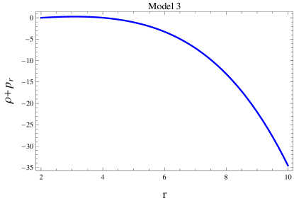
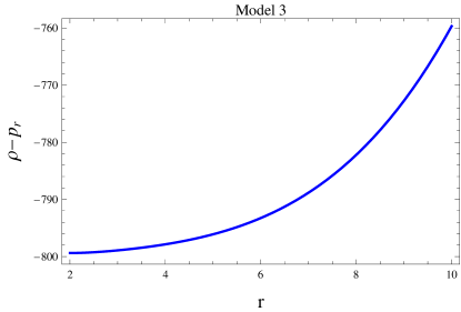
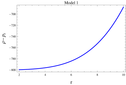
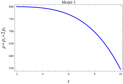
Figure 9: Plots of energy conditions for $\gamma_{3}=2$, $\gamma_{4}=0.002$, $\xi_{3}=0.0003$ $\xi_{4}=0.0005$ and $n=0.001$.

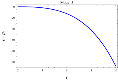
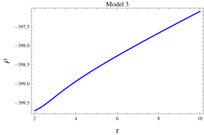
Figure 10: Plots of energy conditions for $\gamma_{3}=-2$, $\gamma_{4}=-0.002$, $\xi_{3}=-0.0003$ $\xi_{4}=-0.0005$ and $n=0.001$

5 Concluding Remarks

Various methods have been used in literature to obtain viable WH structures. One of them is to formulate shape function through different methods and other is to examine the behavior of energy constraints by considering different WSFs. The energy conditions can be used to derive important physical properties of the object. In the present article, we have studied the viable WH geometry through embedding class-I in $f(\mathcal{G})$ gravity. In this perspective, we have built a shape function by employing the Karmarkar condition to check whether WH solutions exist or not in this theory. We have considered three different models of this modified theory to find the exact solutions of static spherical spacetime. We have examined the viability of traversable WH geometry through the energy conditions. The obtained results are summarized as follows

• The newly developed shape function through the Karmarkar condition satisfies all the necessary conditions which ensure the presence of physically viable WH geometry (Figure 1).

• we have discussed embedded diagram to represent the WH structure. We have considered equatorial slice $\theta=\frac{\pi}{2}$ and a fixed moment of time i.e., $t$=constant for spherical symmetry and for the visualization, we embed it into three dimensional Euclidean space. Moreover, one can visualize the upper universe for $h>0$ and the lower universe $h<0$ (Figures 2 and 3).

• Figure 4 shows the graphical behavior of energy conditions for $f(\mathcal{G})=0$. The matter components $(\rho,\rho+p_{r},\rho-p_{t},\rho+p_{r}+2p_{t})$ show negative behavior, indicating the violation of weak, null, dominant and strong energy conditions, respectively. Thus, a viable traversable WH structure can be obtained due to the presence of exotic matter in this gravity model.

• For the first model, we have shown that the fluid parameters violate the energy conditions especially the violation of the null energy condition for both positive/negative values of $\gamma_{1}$, $\xi_{1}$ and $m_{1}$ which gives the existence of exotic matter at the WH throat (Figures 5 and 6). Thus, we have obtained the viable traversable WH geometry for all parametric values.

• For the second model, we have obtained viable traversable WH structure for positive values of model parameters, because the behavior of matter components $(\rho,\rho\pm p_{r},\rho\pm p_{t})$ is negative which ensures the presence of exotic matter at the WH throat (Figure 7). But, for negative values of the model parameters, we have obtained non-traversable WH geometry as the energy conditions are satisfied which gives the existence of normal matter at the WH throat (Figure 6).

• The energy conditions are satisfied for both positive as well as negative values of model parameters, which show that the viable traversable WH geometry exists for the third $f(\mathcal{G})$ model (Figures 9 and 10).

Shamir and Fayyaz [79] examined physically viable WH structure via Karmarkar condition in $f(\mathfrak{R})$ theory and obtained viable WH solutions in the presence of minimum amount of exotic matter. Recently, Sharif and Fatima [56] generalized this work for $f(\mathfrak{R},\mathcal{T})$ theory and obtained viable WH solutions for minimum values of radius. It is noteworthy to mention here that we have found viable WH solutions in $f(\mathcal{G})$ gravity as energy conditions are violated which gives the existence of exotic matter at WH throat. Our investigation has explored traversable WH solutions by incorporating energy conditions, which are composed of energy density and pressure components, encompassing the Gauss-Bonnet terms. Consequently, the WH constructions presented in this manuscript are well established. We conclude that physically viable traversable WH solutions through Karmarkar condition exist in $f(\mathcal{G})$ theory.

Data Availability Statement: No new data were created or analyzed in this study.

References

- [1] L. Flamm, Comments on Einstein’s theory of gravity, Phys. Z. 17(1916)448.
- [2] A. Einstein, N. Rosen, The particle problem in the general theory of relativity, Phys. Rev. 48(1935)73.
- [3] J.A. Wheeler, Geons, Phys. Rev. 97(1955)511.
- [4] R.W. Fuller, J.A. Wheeler, Causality and multiply connected spacetime Phys. Rev. 128(1962)919.
- [5] M.S. Morris, K.S. Thorne, Wormholes in spacetime and their use for interstellar travel: A tool for teaching general relativity Am. J. Phys. 56(1988)395.
- [6] J.P.S. Lemos, F.S.N. Lobo, and S.Q. de Oliveira, Morris-Thorne wormholes with a cosmological constant, Phys. Rev. D 68(2003)064004.
- [7] M. Sharif, I. Fatima, Conformally symmetric traversable wormholes in gravity, Gen. Relativ. Gravit. 48(2016)148.
- [8] M. Cataldo, L. Liempi, P. Rodriguez, Traversable Schwarzschild-like wormholes Eur. Phys. J. C 77(2017)748.
- [9] A.S. Jahromi, H. Moradpour, Static traversable wormholes in Lyra manifold, Int. J. Mod. Phys. D 27(2018)1850024; N. Godani, G.C. Samanta, Traversable wormholes and energy conditions with two different shape functions in gravity, Int. J. Mod. Phys. D 28(2019)1950039; M. Sharif, M.Z. Gul, Traversable wormhole solutions admitting Noether symmetry in Theory, Symmetry 15(2023)684.
- [10] L.P. Eisenhart, Riemannian Geometry (Princeton University Press, 1925).
- [11] K.R. Karmarkar, Gravitational metrics of spherical symmetry and class one, Proc. Indian Acad. Sci. A 27(1948)56.
- [12] P. Bhar, K.N. Singh, T. Manna, A new class of relativistic model of compact stars of embedding class I, Int. J. Mod. Phys. D 26(2017)1750090.
- [13] P. Fuloria, N. Pant, Physical plausibility of cold star models satisfying Karmarkar conditions, Eur. Phys. J. A 53(2017)227.
- [14] G. Abbas, S. Qaisar, W. Javed, M.A. Meraj, Compact stars of emending class one in gravity, Iran J. Sci. Technol. 42(2018)1659.
- [15] S. Gedela, R.K. Bisht, N. Pant, Stellar modelling of PSR J1614-2230 using the Karmarkar condition, Eur. Phys. J. A 54(2018)207.
- [16] P.K. Kuhfittig, Two diverse models of embedding class one, Ann. Phys. 392(2018)63.
- [17] I. Fayyaz, M.F. Shamir, Morris-Thorne wormhole with Karmarkar condition, Chin. J. Phys. 66(2020)553.
- [18] J.D. Bekenstein, Hydrostatic equilibrium and gravitational collapse of relativistic charged fluid balls, Phys. Rev. D 4(1971)2185.
- [19] M. Esculpi, E. Aloma, Conformal anisotropic relativistic charged fluid spheres with a linear equation of state, Eur. Phys. J.C 67(2010)521.
- [20] M. Kalam, et al, Anisotropic strange star with de Sitter spacetime, Eur. Phys. J. C 72(2012)7.
- [21] S.K. Maurya, Y. K. Gupta, S. Ray, and S.R. Chowdhury, Spherically symmetric charged compact stars, Eur. Phys. J. C 75(2015)389.
- [22] M. Sharif, S. Mumtaz, Dynamical instability of gaseous sphere in the Reissner-Nordstrom limit, Gen. Relativ. Gravit. 48(2016)92.
- [23] M. Sharif, F. Javed, Stability of charged thin-shell wormholes with Weyl corrections, Astron. Rep. 65(2021)353.
- [24] S. Perlmutter, et al, Measurements of the Cosmological Parameters and from the First Seven Supernovae at , Astrophys. J. 483(1997)565; Discovery of a supernova explosion at half the age of the Universe, Nature 391(1998)51.
- [25] A.D. Felice, S.R. Tsujikawa, theories, Living Rev. Relativ. 13(2010)3; S. Nojiri, S.D. Odintsov, Unified cosmic history in modified gravity: from theory to Lorentz non-invariant models, Phys. Rep. 505(2011)59; K. Bamba, S. Capozziello, S.I. Nojiri, S.D. Odintsov, Dark energy cosmology, the equivalent description via different theoretical models and cosmography tests, Astrophys. Space Sci. 342(2012)155.
- [26] T. Harko, F.S. Lobo, S.I. Nojiri, S.D. Odintsov, gravity, Phys. Rev. D 84(2011)024020; M. Sharif, M.Z. Gul, Stellar structures admitting Noether symmetries in gravity, Mod. Phys. Lett. A 36(2021)2150214.
- [27] M. Sharif, M.Z. Gul, Dynamics of cylindrical collapse in gravity, Chin. J. Phys. 57(2019)329; Dynamics of perfect fluid collapse in gravity, Int. J. Mod. Phys. D 28(2019)1950054; Study of charged spherical collapse in gravity, Eur. Phys. J. Plus 133(2018)345.
- [28] M. Adeel, M.Z. Gul, S. Rani, A. Jawad, Physical analysis of anisotropic compact stars in gravity, Mod. Phys. Lett. A 38(2023)2350152; S. Rani, M. Adeel, M.Z. Gul, A. Jawad, Anisotropic compact stars admitting karmarkar condition in theory, Int. J. Geom. Methods Mod. Phys. 1(2023)2450033; M.Z. Gul, S. Rani, M. Adeel, A. Jawad, Viable and stable compact stars in theory, Eur. Phys. J. C 84(2024)8.
- [29] M. Sharif, M.Z. Gul, Noether symmetry approach in energy-momentum squared gravity, Phys. Scr. 96(2021)025002.
- [30] M. Sharif, M.Z. Gul, Noether symmetries and anisotropic universe in energy-momentum squared gravity, Phys. Scr. 96(2021)125007.
- [31] M. Sharif, M.Z. Gul, Compact stars admitting noether symmetries in energy-momentum squared gravity, Adv. Astron. 2021(2021)6663502;
- [32] M. Sharif, M.Z. Gul, Scalar field cosmology via Noether symmetries in energy-momentum squared gravity, Chin. J. Phys. 80(2022)58;
- [33] M. Sharif, M.Z. Gul, Noether Symmetries and Some Exact Solutions in Theory, J. Exp. Theor. Phys. 136(2023)436;
- [34] M.Z. Gul, M. Sharif, Traversable wormhole solutions admitting Noether symmetry in Theory, Symmetry 15(2023)684.
- [35] M. Sharif, M.Z. Gul, Stability of the closed Einstein universe in energy-momentum squared gravity, Phys. Scr. 96(2021)105001; Effects of gravity on the stability of anisotropic perturbed Einstein Universe, Pramana J. Phys. 96(2022)153; Stability analysis of the inhomogeneous perturbed Einstein universe in energy-momentum squared gravity, Universe 9(2023)145.
- [36] M. Sharif, M.Z. Gul, Dynamics of spherical collapse in energy-momentum squared gravity, Int. J. Mod. Phys. A 36(2021)2150004.
- [37] M.Z. Gul, M. Sharif, Dynamical analysis of charged dissipative cylindrical collapse in energy-momentum squared gravity, Universe 7(2021)154;
- [38] M. Sharif, M.Z. Gul, Dynamics of charged anisotropic spherical collapse in energy-momentum squared gravity, Chin. J. Phys. 71(2021)365;
- [39] M. Sharif, M.Z. Gul, Role of energy-momentum squared gravity on the dynamics of charged dissipative plane symmetric collapse, Mod. Phys. Lett. A 37(2022)2250005;
- [40] M. Sharif, M.Z. Gul, Study of stellar structures in theory, Int. J. Geom. Methods Mod. Phys. 19(2022)2250012.
- [41] N. Deruelle, On the approach to the cosmological singularity in quadratic theories of gravity: the Kasner regimes, Nucl. Phys. B 327(1989)253; N. Deruelle, L. Farina-Busto, Lovelock gravitational field equations in cosmology, Phys. Rev. D 41(1990)3696.
- [42] B. Bhawal, S. Kar, Lorentzian wormholes in Einstein Gauss-Bonnet theory, Phys. Rev. D 46(1992)2464; N. Deruelle, T. Dolezel, Brane versus shell cosmologies in Einstein and Einstein-Gauss-Bonnet theories, Phys. Rev. D 62(2000)103502.
- [43] S. Nojiri, S.D. Odintsov, Modified Gauss-Bonnet theory as gravitational alternative for dark energy, Phys. Lett. B 631(2005)1.
- [44] A. De Felice, M. Hindmarsh, M. Trodden, Ghosts, instabilities, and superluminal propagation in modified gravity models, J. Cosmol. Astropart. Phys. 08(2006)005.
- [45] G. Cognola, et al, Dark energy in modified Gauss-Bonnet gravity: Late-time acceleration and the hierarchy problem, Phys. Rev. D 73(2006)084007.
- [46] L. Amendola, C. Charmousis, S.C. Davis, Solar system constraints on Gauss-Bonnet mediated dark energy, J. Cosmol. Astropart. Phys. 10(2007)004; A. De Felice, S. Tsujikawa, Solar system constraints on gravity models, Phys. Rev. D 80(2009)063516.
- [47] F.S.N. Lobo, M.A. Oliveria, Wormhole geometries in modified theories of gravity, Phys. Rev. D 80(2009)104012.
- [48] T. Azizi, Wormhole geometries in gravity, Int. J. Theor. Phys. 52(2013)3486.
- [49] M. Sharif, H.I. Fatima, Noncommutative wormhole solutions in gravity, Mod. Phys. Lett. A 30(2015)1550421.
- [50] E. Elizalde, M. Khurshudyan, Wormhole formation in gravity: Varying Chaplygin gas and barotropic fluid, Phys. Rev. D 98(2018)123525.
- [51] M. Sharif, S Hussain, Viable wormhole solutions through Noether symmetry in gravity, Chin. J. Phys. 61(2019)194.
- [52] G. Mustafa, and T.C. Xia, Embedded class solutions of an anisotropic object in Rastall gravity, Int. J. Mod. Phys. A 35(2020) 2050109; Wormhole models with exotic matter in Rastall gravity, Int. J. Geom. Methods Mod. Phys. 17(2020)2050146; G. Mustafa, M.F. Shamir, A. Ashraf, T.C. Xia, Noncommutative wormholes solutions with conformal motion in the background of gravity, Int. J. Geom. Methods Mod. Phys. 17(2020)2050103.
- [53] M. Sharif, M.Z. Gul, Viable wormhole solutions in energy-momentum squared gravity, Eur. Phys. J. Plus 136(2021)503.
- [54] N. Godani, Wormhole solutions in gravity, New Astron. 94(2022)101774.
- [55] A. Malik, F. Mofarreh, A. Zia, A. Ali, Traversable wormhole solutions in the theories of gravity under the Karmarkar condition, Chin. Phys. C 46(2022)095104.
- [56] M. Sharif, A. Fatima, Traversable wormhole solutions admitting Karmarkar condition in theory, Eur. Phys. J. Plus 138(2023)196.
- [57] S.H. Shekh, et al, Observational constraints in accelerated emergent gravity model, Class. Quant. Grav. 40(2023)055011; F. Javed, G. Mustafa, S. Mumtaz, F. Atamurotov, Thermal analysis with emission energy of perturbed black hole in gravity, Nucl. Phys. B 990(2023)116180;
- [58] F. Javed, G. Fatima, S. Sadiq, G. Mustafa, Thermodynamics of Charged Black Hole in Symmetric Teleparallel Gravity, Fortschr. Phys. 2023(2023)2200214; A. Waseem, et al, Impact of quintessence and cloud of strings on self-consistent d-dimensional charged thin-shell wormholes, Eur. Phys. J. C 83(2023)1088.
- [59] M.F. Shamir, I. Fayyaz, Traversable wormhole solutions in gravity via Karmarkar condition, Eur. Phys. J. C 80(2020)1102.
- [60] A. Malik, et al, Traversable wormhole solutions in the theories of gravity under the Karmarkar condition, Chin. Phys. C 46(2022)095104.
- [61] T. Naseer, et al, Constructing traversable wormhole solutions in theory, Chin. J. Phys. 86(2023)350.
- [62] M.Z. Gul, M. Sharif, Study of viable charged wormhole solutions in theory, New Astron. 106(2024)102137.
- [63] B. Sutar, K.L. Mahanta, R.R. Sahoo, Traversable wormhole solutions admitting Karmarkar condition in Lyra manifold, Eur. Phys. J. Plus 138(2023)1115.
- [64] L.A. Anchordoqui, et al, Evolving wormhole geometries, Phys. Rev. D 57(1998)829.
- [65] J. Campbell, A Course on Differential Geometry (Clarenden, Oxford, 1926).
- [66] P.S. Wesson, J.P. de Leon, Kaluza-Klein equations, Einstein equations and an effective energy-momentum tensor, J. Math. Phys. 33(1992)3883.
- [67] S.S. Seahra, P.S. Wesson, Application of the Campbell-Magaard theorem to higher-dimensional physic, Class. Quant. Grav. 20(2003)1321.
- [68] P.S. Wesson, The cosmological constant and quantization in five dimensions, Phys. Lett. B 706(2011)1.
- [69] J.B. Fonseca-Neto, C. Romero, F. Dahia, Godel universe and induced-matter theory, Brazilian J. Phys. 35 (2005)1067.
- [70] S.K. Maurya, M. Govender, Generating physically realizable stellar structures via embedding, Eur. Phys. J. C 77(2017)347.
- [71] S.K. Maurya, S.D. Maharaj, Anisotropic fluid spheres of embedding class one using Karmarkar condition, Eur. Phys. J. C 77(2017)328.
- [72] S.K. Maurya, B.S. Ratanpal, M. Govender, Anisotropic stars for spherically symmetric spacetimes satisfying the Karmarkar condition, Ann. Phys. 382(2017)36.
- [73] S.K. Maurya, Y.K. Gupta, S. Ray, D. Deb, A new model for spherically symmetric charged compact stars of embedding class 1, Eur. Phys. J. C 77(2017)45.
- [74] M. Sharif, M.Z. Gul, Anisotropic compact stars with Karmarkar condition in energy-momentum squared gravity, Gen. Relativ. Gravit. 55(2023)10.
- [75] M. Sharif, M.Z. Gul, Study of Charged Anisotropic Karmarkar Stars in Theory, Fortschritte der Phys. 2023(2023)2200184.
- [76] H.J. Schmidt, Gauss-Bonnet Lagrangian and cosmological exact solutions, Phys. Rev. D 83(2011)083513.
- [77] F. de Felice, Y. Yu, J. Fang, Relativistic charged spheres, Mon. Not. R. Astron. Soc. 277(1995)L17; D. Deb, et al, Study on charged strange stars in gravity, J. Cosmol. Astropart. Phys. 10(2019)070.
- [78] K. Bamba, et al, Finite-time future singularities in modified Gauss-Bonnet and gravity and singularity avoidance, Eur. Phys. J. C 67(2010)295.
- [79] M.F. Shamir, I. Fayyaz, Traversable wormhole solutions in gravity via Karmarkar condition, Eur. Phys. J. C 80(2020)1102.