Slow crossover from superdiffusion to diffusion in isotropic spin chains

Abstract

Finite-temperature spin transport in integrable isotropic spin chains (i.e., spin chains with continuous nonabelian symmetries) is known to be superdiffusive, with anomalous transport properties displaying remarkable robustness to isotropic integrability-breaking perturbations. Using a discrete-time classical model, we numerically study the crossover to conventional diffusion resulting from both noisy and Floquet isotropic perturbations of strength $\lambda$. We identify an anomalously-long crossover time scale $t_{\star}\sim\lambda^{-\alpha}$ with $\alpha\approx 6$ in both cases. We discuss our results in terms of a kinetic theory of transport that characterizes the lifetimes of large solitons responsible for superdiffusion.

Introduction —

High-temperature transport in quantum magnets is usually assumed to be incoherent and diffusive. In this context, the discovery of superdiffusive spin transport with dynamical exponent $z=3/2$ in isotropic integrable quantum spin chains has been especially surprising Žnidarič (2011); Ljubotina et al. (2017, 2019a); Gopalakrishnan and Vasseur (2019); Gopalakrishnan et al. (2019); Jepsen et al. (2020); Wei et al. (2022). While the full picture of superdiffusion in these systems is still coming into focus, a rapidly-growing body of work has elucidated several of its features ( see Bertini et al. (2021); Bulchandani et al. (2021); Gopalakrishnan and Vasseur (2023a, b) for recent reviews). Using recent developments from the theory of Generalized Hydrodynamics (GHD) Bertini et al. (2016); Castro-Alvaredo et al. (2016); Doyon (2020); Bastianello et al. (2022); Doyon et al. (2023), spin superdiffusion has been argued to emerge from the dynamics of large, semi-classical solitons of Goldstone-like nature Gopalakrishnan and Vasseur (2019); Bulchandani (2020); De Nardis et al. (2020a) that are generic in integrable models with continuous non-Abelian symmetries Ilievski et al. (2021). Numerical studies of these models show that the dynamical spin structure factor follows the Kardar-Parisi-Zhang Kardar et al. (1986) scaling form to high accuracy Ljubotina et al. (2019b); Ž. Krajnik et al. (2020); Fava et al. (2020); Dupont and Moore (2020); Scheie et al. (2021); Wei et al. (2022). However, describing higher-order fluctuations seems to require a more complicated fluctuating hydrodynamic theory Krajnik et al. (2024); Ž. Krajnik et al. (2022); De Nardis et al. (2023); Google Quantum AI and Collaborators (2023).

Superdiffusive spin transport was also observed in recent inelastic neutron scattering Scheie et al. (2021), cold atom quantum microscopy Wei et al. (2022), and superconducting qubit Google Quantum AI and Collaborators (2023) experiments. Given that experiments are never described by perfectly integrable systems, it is natural to ask why superdiffusion appears to be so robust to integrability-breaking perturbations. In nearly integrable systems, the short-time dynamics are integrable, but at sufficiently long times, the dynamics become chaotic with diffusive transport properties Friedman et al. (2020); Durnin et al. (2021); Bastianello et al. (2020, 2021). The nature of this crossover from superdiffusive to diffusive spin transport in nearly-integrable isotropic spin chains remains poorly understood. Perturbative arguments indicate that the symmetry of the integrability-breaking perturbation is crucial: for anisotropic perturbations (those that break spin-rotation symmetry), the crossover timescales follow generic Fermi’s Golden Rule (FGR) predictions and scale with the square of the perturbation strength De Nardis et al. (2021). In contrast, the timescales that characterize the crossover to diffusion associated with applying isotropic perturbations are known to be much slower De Nardis et al. (2021); Roy et al. (2023a, b); McRoberts et al. (2022a), but these timescales have yet to be precisely characterized. This crossover is so slow that it remains controversial whether transport in the long-time limit is indeed diffusive  De Nardis et al. (2020b); Glorioso et al. (2021); Claeys et al. (2022). The primary obstacles to numerically observing the crossover to diffusion for isotropic perturbations have been the computational expense of simulating quantum systems and the robustness of superdiffusion with respect to isotropic perturbations, which together make accessing the crossover timescale difficult De Nardis et al. (2021); Nandy et al. (2023). Even for classical spin chains simulated using standard numerical techniques like Runge-Kutta methods, superdiffusive transport in models like the Ishimori spin chain Ishimori (1982) survives for all numerically-accessible timescales in the presence of isotropic perturbations Roy et al. (2023a, b); McRoberts et al. (2022a).

In this letter, we employ an integrability-preserving discrete time integration scheme Ž. Krajnik and Prosen (2020); Ž. Krajnik et al. (2020) that allows us to reach times up to $t_{\rm max}=2^{16}$ for systems of $N=200000$ spins, which is sufficient to observe the long timescale associated with the superdiffusive-to-diffusive crossover for isotropic perturbations. For both noisy and Floquet isotropic perturbations of strength $\lambda$, we observe a crossover to conventional diffusion $t_{\star}\sim\lambda^{-\alpha}$ that is compatible with $\alpha=6$. For noisy chains, this slow timescale can be understood in terms of a kinetic theory that characterizes the lifetimes of the large solitons responsible for spin transport.

Isotropic spin chains —

For concreteness we focus on integrable spin chains with Hamiltonian $H_{0}$, which are invariant under spin-rotation symmetry, perturbed by some spin-rotation-invariant integrability-breaking term $V$ of strength $\lambda$:

$$H=(1-\lambda)H_{0}+\lambda V.$$ (1)

Here $\lambda\in[0,1]$ is a parameter interpolating between integrable ($\lambda=0$) and purely non-integrable ($\lambda=1$) dynamics. Our analysis is general for any integrable spin chain, classical or quantum, that is invariant under some continuous nonabelian symmetry. However, since diffusion emerges on very long timescales, we simulate models for which one can reliably study very late times. Thus, first, we consider classical spin chains: Each site $n$ along the classical spin chain hosts an $O(3)$ vector of unit norm $\vec{S}_{n}=(S^{x}_{n},S^{y}_{n},S^{z}_{n})$ with canonical Poisson brackets $\{S^{i}_{n},S^{j}_{m}\}=\epsilon_{ijk}S^{k}_{n}\delta_{nm}$, subject to nearest-neighbor ferromagnetic interactions. Second, to avoid the accumulation of truncation errors in schemes like Runge-Kutta, we will simulate a discrete-time, Trotterized form of the dynamics. To this end we will exploit the existence of Trotterizations of classical spin chains that preserve integrability Ž. Krajnik and Prosen (2020); Ž. Krajnik et al. (2020, 2022).

In the remainder of this work, the integrable dynamics will be generated by an integrable Trotterization Ž. Krajnik and Prosen (2020); Ž. Krajnik et al. (2020, 2022) of the classical Ishimori Hamiltonian $H_{0}=-\sum_{n}\mathrm{ln}(1+\vec{S}_{n}\cdot\vec{S}_{n+1})$ Ishimori (1982). The isotropic integrability-breaking perturbation will be an (again Trotterized) Heisenberg interaction $V=-\sum_{n}g_{n}(t)\vec{S}_{n}\cdot\vec{S}_{n+1}$. We will consider two cases: (i) perturbations that are noisy, where $g_{n}(t)$ will be taken to be random variables uncorrelated in both space and time, $\overline{g_{n}(t)g_{m}(t^{\prime})}=\delta_{nm}\delta(t-t^{\prime})$, where $\overline{O}$ denotes the average of $O$ over noise, and (ii) perturbations that are time-periodic, for which $g_{n}(t)=1$.

Spin transport —

Numerical, theoretical and experimental studies have shown that spin transport in the integrable limit $\lambda=0$ is known to be superdiffusive, while energy transport is purely ballistic Žnidarič (2011); Ljubotina et al. (2017, 2019a); Gopalakrishnan and Vasseur (2019); Gopalakrishnan et al. (2019); Scheie et al. (2021); Jepsen et al. (2020); Wei et al. (2022). For simplicity, we will focus on the infinite-temperature regime where spins are initialized at random, although our conclusions carry over to arbitrary finite temperatures. In order to characterize spin transport, we will focus on fluctuations of spin transfer across a given bond in a background equilibrium state. We define spin transfer as the time-integrated spin current across the link between sites $n$ and $n+1$, $Q(t)=\int_{0}^{t}dtj_{n}(t)$, where $j_{n}(t)$ is the spin current between sites $n$ and $n+1$, defined by the continuity equation $\partial_{t}S^{z}_{n}+j_{n+1}-j_{n}=0$. We invoke translation invariance and average this quantity over each bond $n$ to improve statistics. Since there is no net spin transfer in a background equilibrium state, the thermal average $\langle Q(t)\rangle=0$ vanishes. Fluctuations in spin transfer can be used to characterize spin transport through the relation

$$\langle Q(t)^{2}\rangle\sim t^{1/z},$$ (2)

where $z$ is the dynamical exponent, which characterizes transport by relating space and time scaling through $t\sim x^{z}$. For diffusive transport, we see the dynamical exponent $z=2$, whereas we see $z=3/2$ in integrable isotropic chains, corresponding to superdiffusive (faster than diffusive) transport with an effective time-dependent diffusion constant $D(t)\sim t^{1/3}$. In order to characterize the crossover from $z=3/2$ to $z=2$ upon applying an integrability-breaking perturbation, we will define the time-dependent dynamical exponent as the logarithmic derivative $z(t)=\left(\frac{d\ln\langle Q^{2}\rangle}{d\ln t}\right)^{-1}$.

As a consistency check, we also characterize spin transport and the crossover to diffusion using the spin autocorrelation function $C(t)=\langle S^{z}_{n}(t)S^{z}_{n}(0)\rangle\sim t^{-1/z}$. We extract the dynamical exponent $z$ from $C(t)$ and observe results compatible with those discussed below (see sup ). Since transport becomes diffusive at long times with $C(t)\sim 1/\sqrt{D(\lambda)t}$, the autocorrelation function can also be used to compute the diffusion constant $D(\lambda)$ from $\lim_{t\to\infty}\left(\sqrt{t}~{}C(t)\right)$ Glorioso et al. (2021).

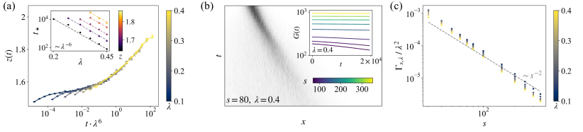
Figure 1: Crossover to diffusion in noisy spin chains. (a) Effective time-dependent dynamical exponent $z(t)$ extracted from spin transfer fluctuations, showing a crossover from $z=3/2$ (superdiffusion, integrable case) to $z=2$ (diffusion) for different values of the integrability-breaking parameter $\lambda$. Data is averaged over at least 2000 samples (including random initial states and different realizations of the noisy perturbation), and we used a timestep of $\tau=0.25$. We observe a collapse as a function of the rescaled variable $t\lambda^{6}$, indicating a crossover time scale $t_{\star}\sim\lambda^{-6}$. Inset: time scale $t_{\star}(\lambda)$ at which $z(t)$ reaches some set value of $z$ (color scale), showing a clear power-law scaling $t_{\star}\sim\lambda^{-6}$. (b) Example of soliton “melting” in the presence of a noisy perturbation. Inset: Exponential decay of the IPR $G(t)$ for different soliton sizes $s$. (c) Soliton decay rates in the vacuum, showing a scaling compatible with $\Gamma_{s,\lambda}\sim\lambda^{2}/s^{2}$.

Noisy perturbations: numerics —

The discrete-time model used here can be efficiently simulated up to very long times without accumulating Trotter errors, allowing us to reach maximum times of $t=2^{16}$ for systems up to $N=200000$ spins, which is sufficient to observe the crossover to diffusion for noisy isotropic perturbations. The effective time-dependent dynamical exponent $z(t)$ extracted from the spin transfer shows a clear crossover from $z=3/2$ to $z=2$ at long times (Fig. 1a). We find that the crossover occurs over a long time scale $t_{\star}\sim\lambda^{-\alpha}$ with an exponent consistent with $\alpha=6$. We additionally extract the diffusion constant $D(\lambda)$ from the autocorrelation function $C(t)=\frac{1}{N}\sum_{n}\langle S_{n}^{z}(t)S_{n}^{z}(0)\rangle$, and find that it scales as $D(\lambda)\sim\lambda^{-2}$ (see sup ). Since matching the diffusive and integrable behaviors at $t=t_{\star}$ gives $D(\lambda)\sim t_{\star}^{1/3}\sim\lambda^{-\alpha/3}$ for $t_{\star}\sim\alpha$, the scaling $D(\lambda)\sim\lambda^{-2}$ is also consistent with $t_{\star}\sim\lambda^{-6}$ sup . (In contrast, a process by which the solitons decay in an $s$-independent way through Golden Rule processes yields a crossover time $t_{\star}\sim\lambda^{-2}$ and a diffusion constant $D(\lambda)\sim\lambda^{-2/3}$, consistent with numerical data on anisotropic perturbations De Nardis et al. (2021); sup .)

Kinetic theory —

To understand this unusually long crossover time scale, we turn to a kinetic theory of the quasiparticles responsible for superdiffusion in the integrable case. In integrable isotropic spin chains, superdiffusive transport with $z=3/2$ is well established in terms of the system’s quasiparticle excitations Gopalakrishnan and Vasseur (2019); Gopalakrishnan et al. (2019); De Nardis et al. (2019, 2019, 2020a); Ilievski et al. (2021). In classical chains, these quasiparticles are infinitely long-lived solitons which remain stable even at high temperatures. Solitons are characterized by their size $s$, a parameter that is quantized in quantum spin chains and continuous in classical chains. These solitons have velocity $v_{s}\sim 1/s$, so large solitons move slowly, and occur with density $\rho_{s}\sim 1/s^{3}$ in thermal equilibrium Ilievski et al. (2018). They also carry spin $m_{s}=s$ in the vacuum, although this net magnetization can be screened in thermal states by a background consisting of other overlapping solitons Sachdev and Damle (1997); Damle and Sachdev (1998); Ilievski et al. (2018). Integrability results show that solitons are screened at a rate $\Gamma^{0}_{s}\sim s^{-3}$ Gopalakrishnan and Vasseur (2019); Gopalakrishnan et al. (2019); Agrawal et al. (2020). This means that at a given time $t$, small solitons with $s\ll s_{\star}(t)\sim t^{1/3}$ are fully screened and carry a net magnetization $m_{s}=0$, and so they do not contribute to spin transport. On the other hand, “giant” solitons $s\gg s_{\star}(t)\sim t^{1/3}$ remain charged and dominate transport. Combined with the slow velocity $v_{s}\sim 1/s$ of giant solitons, this screening mechanism is responsible for the superdiffusion exponent $z=3/2$ in integrable isotropic chains Gopalakrishnan and Vasseur (2019).

Soliton decay rates —

In the presence of an integrability-breaking perturbation of strength $\lambda\neq 0$, solitons acquire a finite lifetime due to both vacuum decay processes and backscattering from collisions. The finite lifetime of a soliton of size $s$ subjected to an integrability-breaking perturbation is characterized by the decay rate $\Gamma_{s,\lambda}$, which we expect to take the form $\Gamma_{s,\lambda}\sim\sum_{n}\lambda^{\alpha_{n}}s^{-\beta_{n}},$ with each term indexed by $n$ corresponding to a different decay process. Note any process with $\beta_{n}\geq 3$ will occur slower than the integrable screening process $\Gamma^{0}_{s}\sim s^{-3}$ for large solitons and is thus irrelevant. The crossover to diffusion can be understood as a competition between the integrable screening rate $\Gamma^{0}_{s}\sim s^{-3}$ and the perturbation-induced decay rate $\Gamma_{s,\lambda}$. The crossover occurs when perturbative contributions to a soliton’s decay rate $\Gamma_{s,\lambda}$ overpower the screening rate $\Gamma^{0}_{s}$; that is, the time at which the perturbative decay rate scales like $\Gamma_{s,\lambda}\sim s^{-3}$.

The task of understanding the crossover therefore reduces to finding the leading-order term of the decay rate $\Gamma_{s,\lambda}$ induced by a noisy isotropic perturbation. In general, analytically evaluating $\Gamma_{s,\lambda}$ is very complicated, even perturbatively. We study this question numerically by considering the decay of a single soliton of size $s$ in a vacuum background state, corresponding to an initial state $(S^{x}_{n},S^{y}_{n},S^{z}_{n})=(\sqrt{1-(S_{n}^{z})^{2}}\cos\phi_{n},\sqrt{1-(S_{n}^{z})^{2}}\sin\phi_{n},S_{n}^{z})$ with

$$S_{n}^{z}=\tanh^{2}\left(\frac{n}{2s}\right),$$ (3)

and $\phi_{n}=\arctan\left(\tanh\frac{n}{2s}\right)+\frac{n}{2s}$ Lakshmanan et al. (1976). This initial state corresponds to an exact right-moving soliton in the Ishimori chain with interaction $\mathrm{ln}(1+\vec{S}_{n}\cdot\vec{S}_{n+1})$ – left-movers can be obtained by shifting the phase $\phi_{n}\rightarrow\phi_{n}+\pi/2$. In the context of our discrete time numerics, this initial state is not technically an exact soliton (even for $\lambda=0$), but it has a very strong overlap with the solitons of the discrete-time model.

In the integrable case ($\lambda=0$), solitons propagate without decaying. Applying a noisy perturbation of strength $\lambda\neq 0$ causes a giant soliton to disintegrate into small solitons that diffuse through backscattering. To quantify this decay, we introduce the inverse participation ratio (IPR) $G(t)=\sum_{n}(S_{n}^{z}(t)-1)^{2}$. Spin conservation fixes $\sum_{n}(S_{n}^{z}-1)$ as a time-independent constant of order $s$; therefore, $G(t)$ provides a metric to quantify the localization of soliton. For a localized soliton, $G(t)$ remains a constant of order $s$, while for a delocalized soliton it decays with system size as $1/L$. For large systems and long times, we observe an exponential decay $G(t)\sim{\rm e}^{-\Gamma_{s,\lambda}t}$, which allows us to extract the decay rates $\Gamma_{s,\lambda}$ numerically for various soliton sizes $s$ and perturbation strengths $\lambda$ (Fig. 1(b)). We find that

$$\Gamma_{s,\lambda}\sim\frac{\lambda^{2}}{s^{2}},$$ (4)

in agreement with recent perturbative arguments (Fig. 1(c)) De Nardis et al. (2021). The long lifetimes $\sim s^{2}$ of large solitons can be understood in terms of the Goldstone-like nature of the solitons (3): matrix elements of isotropic perturbations are suppressed as $1/s$ acting on a soliton of size $s$ De Nardis et al. (2021). Comparing the decay rates (4) to the integrable screening rates, we find the crossover soliton size $s_{\star}\sim\lambda^{-2}$, and the crossover time scale

$$t_{\star}\sim\lambda^{-6},$$ (5)

in agreement with the anomalously long time scale observed in our transport data (Fig. 1(a)) and extracted diffusion constant (see sup ).

While the vacuum decay rates (4) fully explain the crossover time scale $t_{\star}\sim\lambda^{-6}$, they also lead to logarithmic corrections to diffusion, since the giant solitons’ lifetime $\sim s^{2}$ in the vacuum is long enough to lead to anomalous behavior De Nardis et al. (2021). Whether interactions can induce decay rates $\sim s^{-\alpha}$ with $\alpha<2$ that restore diffusion remains an important question.

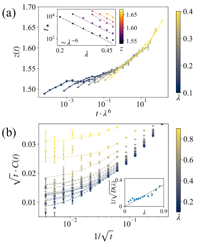
Figure 2: Crossover to diffusion for Floquet perturbations. (a) dynamical exponent $z(t)$ extracted from fluctuations of spin transfer plotted against $t\lambda^{6}$. Data is averaged over at least 4000 random initial states for a system size of $N=200000$ sites with a timestep $\tau=0.25$. We observe a curve collapse is compatible with crossover timescale $t_{\star}\sim\lambda^{-6}.$ Inset: timescale $t_{\star}$ at which a particular value $z(t_{\star})$ is reached for different lambdas, demonstrating power-law scaling $\sim\lambda^{-6}$. (b) Adjusted autocorrelation function $\sqrt{t}C(t)=\frac{\sqrt{t}}{N}\sum_{n}\langle S_{n}^{z}(t)S_{n}^{z}(0)\rangle$ plotted against $1/\sqrt{t}$. Curves corresponding to large perturbations of strength $\lambda>0.5$ are averaged over at least 2000 random initial states, while small perturbations $\lambda\leq 0.5$ are averaged over at least 4000 random initial states. Dashed lines correspond to fitting $\sqrt{t}C(t)$ for $t\geq 256$ with its standard form at late times, $\sqrt{t}C(t)\sim 1/\sqrt{D(\lambda)}+A/\sqrt{t}+B/t+\dots$, where $D(\lambda)$ is the diffusion constant up to irrelevant numerical prefactors Glorioso et al. (2021). Inset: $1/\sqrt{D(\lambda)}$ extracted by fitting the adjusted autocorrelation function $\sqrt{t}C(t)$. The linear scaling of $1/\sqrt{D(\lambda)}$ is consistent with a crossover timescale of $t_{\star}\sim\lambda^{-6}$ sup .

Floquet perturbations —

The previous section considered noisy perturbations $V(t)=-\sum_{n}g_{n}(t)\vec{S}_{n}\cdot\vec{S}_{n+1}$, with $g_{n}(t)$ uncorrelated random variables in both space and time. We now consider non-noisy (Floquet) perturbations with $g_{n}(t)=1$. The crossover associated with a noisy perturbation is primarily driven by the vacuum decay rate $\Gamma_{s,\lambda}\sim\lambda^{2}/s^{2}$; however, in the absence of noise, isolated solitons remain stable even in the non-integrable classical Heisenberg chain McRoberts et al. (2022b). The largest contribution to the decay rate must therefore arise from many-body soliton scattering processes; this term should also exist in the decay rate for the noisy perturbations but is masked by the leading-order contribution from the vacuum decay process. Therefore, we expect the crossover timescale associated with Floquet perturbations to be at least as slow as the noisy crossover timescale $t_{\star}\sim\lambda^{-6}$, if not slower. This picture is consistent with the recent numerical works on classical spin chains Roy et al. (2023a, b); McRoberts et al. (2022a), which were unable to observe a systematic crossover towards diffusion on timescales accessible by standard continuous-time integration schemes like adaptive Runge-Kutta methods.

The discrete-time numerics used here are able to access very long times without finite time-step errors, which allows us to observe timescales inaccessible to Runge-Kutta setups. Even so, we observe a curve collapse for the dynamical exponent $z(t)$ that is slower than the noisy case but still consistent with $t_{\star}\sim\lambda^{-\alpha}$ scaling with $\alpha\approx 6$ (Fig. 2a). For consistency, we extract the diffusion constant $D(\lambda)$ from the autocorrelation function using the same method as described for the noisy perturbation, which is also compatible with $t_{\star}\sim\lambda^{-6}$ scaling (Fig. 2b). We note that our data cannot definitively exclude a different exponent in the true scaling limit $t\to\infty$ and $\lambda\to 0$, and different values of $\alpha$ lead to acceptable collapses as well (see sup ).

As previously discussed, we expect that the crossover to diffusion is driven by collisions between multiple solitons; however, since the IPR is not a meaningful metric for a finite density of solitons, it is difficult to determine collision decay rates using the same methods as were used to extract the noisy vacuum decay rate. By simulating experiments in which large solitons first interact with a non-trivial background under $\lambda\neq 0$ dynamics, and then filtering out the background by setting $\lambda=0$ and allowing it to “expand” into a vacuum region, we are able to show that the soliton lifetime increases with $s$, although the data are too noisy to extract a reliable exponent sup . We note that the crossover scale $t_{\star}\sim\lambda^{-6}$ is compatible with higher-order perturbative decay rates $\Gamma_{s,\lambda}\sim\lambda^{2(n+1)}s^{n-2}$ for any $n$. On general grounds, we expect the collisions between $s$-sized solitons at large $s$ and $O(1)$-sized solitons to scale as $1/s^{2}$, since a small soliton experiences a large one as a local vacuum rotation. In effect, a thermal background of small solitons acts as noise on the large ones, relating the Floquet and noisy cases. This process would once again lead to logarithmically corrected diffusion. Any higher-order processes with $n>0$, if present, would lead to a full crossover to diffusion. Determining the form of the decay rates that emerge from interactions remains an important challenge for future work.

Discussion — We have numerically observed the slow crossover from superdiffusive to diffusive transport for isotropically-perturbed integrable classical spin chains, with a crossover timescale $t_{\star}\sim\lambda^{-\alpha}$ with $\alpha\approx 6$. Our ability to reach this anomalously long crossover timescale is due to the classical discrete time algorithm used in this work, in contrast to previous work that studied this question with matrix-product states or classical continuous time numerical methods. The $t_{\star}\sim\lambda^{-6}$ scaling holds for both noisy and Floquet perturbations. While the exponent $\alpha=6$ is expected perturbatively in the noisy case, and has a heuristic justification in the clean case, a full explanation of the crossover to diffusion in either case requires analyzing the decay rates that arise from $n$-body soliton scattering processes, and presents an important challenge for future theoretical work. For example it is possible that the crossover to diffusion happens in multiple stages, with an intermediate regime of logarithmically corrected diffusion that gets parametrically large in $\lambda$. We note that although our numerics are consistent with an exponent $\alpha\approx 6$ for Floquet perturbations, we cannot conclusively exclude other values of $\alpha$ in the limit of $\lambda\rightarrow 0$ and hope that future theoretical and numerical advances will pinpoint the exact exponent.

Note:

During the completion of this work, we became aware of a related work by Adam McRoberts and Roderich Moessner McRoberts and Moessner reporting a crossover timescale of $t_{\star}\sim\lambda^{-3}$ in an energy-conserving model and analyzing its temperature dependence. Future work would be needed to understand why the crossovers in both models appear to be dominated by different decay processes on accessible time scales.

See pages 1 of suppmat.pdf

See pages 2 of suppmat.pdf

See pages 3 of suppmat.pdf

See pages 4 of suppmat.pdf

See pages 5 of suppmat.pdf

See pages 6 of suppmat.pdf

References

- Žnidarič (2011) M. Žnidarič, Phys. Rev. Lett. 106, 220601 (2011).
- Ljubotina et al. (2017) M. Ljubotina, M. Žnidarič, and T. Prosen, Nature Communications 8, 16117 EP (2017).
- Ljubotina et al. (2019a) M. Ljubotina, L. Zadnik, and T. Prosen, Physical Review Letters 122 (2019a), 10.1103/physrevlett.122.150605.
- Gopalakrishnan and Vasseur (2019) S. Gopalakrishnan and R. Vasseur, Phys. Rev. Lett. 122, 127202 (2019).
- Gopalakrishnan et al. (2019) S. Gopalakrishnan, R. Vasseur, and B. Ware, Proceedings of the National Academy of Sciences 116, 16250 (2019).
- Jepsen et al. (2020) P. N. Jepsen, J. Amato-Grill, I. Dimitrova, W. W. Ho, E. Demler, and W. Ketterle, Nature 588, 403 (2020).
- Wei et al. (2022) D. Wei, A. Rubio-Abadal, B. Ye, F. Machado, J. Kemp, K. Srakaew, S. Hollerith, J. Rui, S. Gopalakrishnan, N. Y. Yao, I. Bloch, and J. Zeiher, Science 376, 716 (2022).
- Bertini et al. (2021) B. Bertini, F. Heidrich-Meisner, C. Karrasch, T. Prosen, R. Steinigeweg, and M. Žnidarič, Rev. Mod. Phys. 93, 025003 (2021).
- Bulchandani et al. (2021) V. B. Bulchandani, S. Gopalakrishnan, and E. Ilievski, Journal of Statistical Mechanics: Theory and Experiment 2021, 084001 (2021).
- Gopalakrishnan and Vasseur (2023a) S. Gopalakrishnan and R. Vasseur, Reports on Progress in Physics 86, 036502 (2023a).
- Gopalakrishnan and Vasseur (2023b) S. Gopalakrishnan and R. Vasseur, “Superdiffusion from nonabelian symmetries in nearly integrable systems,” (2023b), arXiv:2305.15463 [cond-mat.stat-mech] .
- Bertini et al. (2016) B. Bertini, M. Collura, J. De Nardis, and M. Fagotti, Phys. Rev. Lett. 117, 207201 (2016).
- Castro-Alvaredo et al. (2016) O. A. Castro-Alvaredo, B. Doyon, and T. Yoshimura, Phys. Rev. X 6, 041065 (2016).
- Doyon (2020) B. Doyon, SciPost Physics Lecture Notes (2020), 10.21468/scipostphyslectnotes.18.
- Bastianello et al. (2022) A. Bastianello, B. Bertini, B. Doyon, and R. Vasseur, Journal of Statistical Mechanics: Theory and Experiment 2022, 014001 (2022).
- Doyon et al. (2023) B. Doyon, S. Gopalakrishnan, F. Møller, J. Schmiedmayer, and R. Vasseur, “Generalized hydrodynamics: a perspective,” (2023), arXiv:2311.03438 [cond-mat.stat-mech] .
- Bulchandani (2020) V. B. Bulchandani, Phys. Rev. B 101, 041411 (2020).
- De Nardis et al. (2020a) J. De Nardis, S. Gopalakrishnan, E. Ilievski, and R. Vasseur, Phys. Rev. Lett. 125, 070601 (2020a).
- Ilievski et al. (2021) E. Ilievski, J. De Nardis, S. Gopalakrishnan, R. Vasseur, and B. Ware, Phys. Rev. X 11, 031023 (2021).
- Kardar et al. (1986) M. Kardar, G. Parisi, and Y.-C. Zhang, Phys. Rev. Lett. 56, 889 (1986).
- Ljubotina et al. (2019b) M. Ljubotina, M. Žnidarič, and T. Prosen, Phys. Rev. Lett. 122, 210602 (2019b).
- Ž. Krajnik et al. (2020) Ž. Krajnik, E. Ilievski, and T. Prosen, SciPost Phys. 9, 038 (2020).
- Fava et al. (2020) M. Fava, B. Ware, S. Gopalakrishnan, R. Vasseur, and S. A. Parameswaran, Phys. Rev. B 102, 115121 (2020).
- Dupont and Moore (2020) M. Dupont and J. E. Moore, Phys. Rev. B 101, 121106 (2020).
- Scheie et al. (2021) A. Scheie, N. E. Sherman, M. Dupont, S. E. Nagler, M. B. Stone, G. E. Granroth, J. E. Moore, and D. A. Tennant, Nature Physics 17, 726 (2021).
- Krajnik et al. (2024) i. c. v. Krajnik, J. Schmidt, E. Ilievski, and T. c. v. Prosen, Phys. Rev. Lett. 132, 017101 (2024).
- Ž. Krajnik et al. (2022) Ž. Krajnik, E. Ilievski, and T. a. Prosen, Physical Review Letters 128 (2022), 10.1103/physrevlett.128.090604.
- De Nardis et al. (2023) J. De Nardis, S. Gopalakrishnan, and R. Vasseur, Phys. Rev. Lett. 131, 197102 (2023).
- Google Quantum AI and Collaborators (2023) Google Quantum AI and Collaborators, “Dynamics of magnetization at infinite temperature in a heisenberg spin chain,” (2023), arXiv:2306.09333 [quant-ph] .
- Friedman et al. (2020) A. J. Friedman, S. Gopalakrishnan, and R. Vasseur, Phys. Rev. B 101, 180302 (2020).
- Durnin et al. (2021) J. Durnin, M. J. Bhaseen, and B. Doyon, Phys. Rev. Lett. 127, 130601 (2021).
- Bastianello et al. (2020) A. Bastianello, J. De Nardis, and A. De Luca, Phys. Rev. B 102, 161110 (2020).
- Bastianello et al. (2021) A. Bastianello, A. D. Luca, and R. Vasseur, Journal of Statistical Mechanics: Theory and Experiment 2021, 114003 (2021).
- De Nardis et al. (2021) J. De Nardis, S. Gopalakrishnan, R. Vasseur, and B. Ware, Phys. Rev. Lett. 127, 057201 (2021).
- Roy et al. (2023a) D. Roy, A. Dhar, H. Spohn, and M. Kulkarni, “Nonequilibrium spin transport in integrable and non-integrable classical spin chains,” (2023a), arXiv:2306.07864 [cond-mat.stat-mech] .
- Roy et al. (2023b) D. Roy, A. Dhar, H. Spohn, and M. Kulkarni, Phys. Rev. B 107, L100413 (2023b).
- McRoberts et al. (2022a) A. J. McRoberts, T. Bilitewski, M. Haque, and R. Moessner, Phys. Rev. B 105, L100403 (2022a).
- De Nardis et al. (2020b) J. De Nardis, M. Medenjak, C. Karrasch, and E. Ilievski, Phys. Rev. Lett. 124, 210605 (2020b).
- Glorioso et al. (2021) P. Glorioso, L. V. Delacrétaz, X. Chen, R. M. Nandkishore, and A. Lucas, SciPost Phys. 10, 015 (2021).
- Claeys et al. (2022) P. W. Claeys, A. Lamacraft, and J. Herzog-Arbeitman, Phys. Rev. Lett. 128, 246603 (2022).
- Nandy et al. (2023) S. Nandy, Z. Lenarčič, E. Ilievski, M. Mierzejewski, J. Herbrych, and P. Prelovšek, Phys. Rev. B 108, L081115 (2023).
- Ishimori (1982) Y. Ishimori, Journal of the Physical Society of Japan 51, 3417 (1982).
- Ž. Krajnik and Prosen (2020) Ž. Krajnik and T. Prosen, Journal of Statistical Physics 179, 110–130 (2020).
- (44) See Supplementary Information for further information on discrete time numerics, anisotropic perturbations, additional autocorrelation function data, a discussion of the choice of scaling parameter, and numerics for many-body soliton decay processed for Floquet perturbations.
- De Nardis et al. (2019) J. De Nardis, M. Medenjak, C. Karrasch, and E. Ilievski, Phys. Rev. Lett. 123, 186601 (2019).
- Ilievski et al. (2018) E. Ilievski, J. De Nardis, M. Medenjak, and T. Prosen, Phys. Rev. Lett. 121, 230602 (2018).
- Sachdev and Damle (1997) S. Sachdev and K. Damle, Phys. Rev. Lett. 78, 943 (1997).
- Damle and Sachdev (1998) K. Damle and S. Sachdev, Phys. Rev. B 57, 8307 (1998).
- Agrawal et al. (2020) U. Agrawal, S. Gopalakrishnan, R. Vasseur, and B. Ware, Phys. Rev. B 101, 224415 (2020).
- Lakshmanan et al. (1976) M. Lakshmanan, T. W. Ruijgrok, and C. Thompson, Physica A: Statistical Mechanics and its Applications 84, 577 (1976).
- McRoberts et al. (2022b) A. J. McRoberts, T. Bilitewski, M. Haque, and R. Moessner, Phys. Rev. E 106, L062202 (2022b).
- (52) A. J. McRoberts and R. Moessner, “Long lifetime of superdiffusion in non-integrable spin chains,” .