Versatile Mixed Methods for Compressible Flows

Abstract

Versatile mixed finite element methods were originally developed by Chen and Williams for isothermal incompressible flows in “Versatile mixed methods for the incompressible Navier-Stokes equations,” Computers & Mathematics with Applications, Volume 80, 2020. Thereafter, these methods were extended by Miller, Chen, and Williams to non-isothermal incompressible flows in “Versatile mixed methods for non-isothermal incompressible flows,” Computers & Mathematics with Applications, Volume 125, 2022. The main advantage of these methods lies in their flexibility. Unlike traditional mixed methods, they retain the divergence terms in the momentum and temperature equations. As a result, the favorable properties of the schemes are maintained even in the presence of non-zero divergence. This makes them an ideal candidate for an extension to compressible flows, in which the divergence does not generally vanish. In the present article, we finally construct the fully-compressible extension of the methods. In addition, we demonstrate the excellent performance of the resulting methods for weakly-compressible flows that arise near the incompressible limit, as well as more strongly-compressible flows that arise near Mach 0.5.

1 Introduction

In this paper, we discuss the discretization of the compressible Navier-Stokes equations using ‘versatile mixed finite element methods’. This paper introduces an important extension to previous mixed methods for solving the isothermal incompressible Navier-Stokes equations [1], and the non-isothermal incompressible Navier-Stokes equations [2]. While mixed finite element methods have seen significant interest for applications to incompressible flows, there has been very limited interest in applying them to compressible flows. This is primarily due to the greater complexity and non-linearity of compressible flows relative to incompressible flows. There are many numerical methods which have the potential to address this challenge. However, in this work we will focus on finite element methods due to their compact stencil, ability to operate on unstructured grids, high-order accuracy, and strong mathematical foundations.

Broadly speaking, we can classify finite element methods for simulating fluids into different categories based on their stabilization strategies. There are at least five stabilization strategies of immediate interest to us: i) residual-based stabilization, ii) numerical-flux-based stabilization, iii) entropy-based stabilization, iv) kinetic-energy-based stabilization, and v) inf-sup stabilization. Often, combinations of these stabilization strategies are used within the same finite element method. In what follows, we will describe each stabilization strategy, its strengths and weaknesses, and then provide some examples of finite element methods which use the strategy. Based on this broad discussion, we will identify the particular stabilization strategies which we deem most effective. Then, we will explain how versatile mixed methods achieve stability using these particular strategies, and how our methods fit into the general landscape of finite element methods for weakly- and fully-compressible flows.

Note: for those readers who are familiar with finite element stabilization strategies, they may skip section 1.1, and proceed directly to section 1.2.

1.1 Background

Let us begin by considering a residual-based stabilization strategy. For example, the standard continuous Galerkin (CG) finite element formulation is frequently augmented with a stabilization term which contains the product of the residual operator applied to the solution, a symmetric positive definite matrix, and a residual operator applied to the test functions. Streamline Upwind Petrov-Galerkin (SUPG) methods [3, 4, 5] use this strategy for stabilization, as they leverage a convection-based residual operator for the test functions. The SUPG methods are known for their excellent performance in convection-dominated flows, although they are not guaranteed to remain stable in the diffusive limit. Galerkin-Least-Squares (GLS) methods [5] are closely related to SUPG methods, with the caveat that they apply the full residual operator (both its advective and diffusive parts) to the test functions. See [6, 7, 8] for a general discussion of least-squares finite element methods. These methods often perform well in both convection- and diffusion-dominated flows, as they are mathematically guaranteed to maintain stability in both settings. Lastly, the Variational Multiscale (VMS) methods [9, 10, 11, 12] are closely related to GLS methods, with the caveat that they apply the adjoint of the full residual operator to the test functions. In contrast to SUPG and GLS methods, these methods achieve adjoint consistency, although they are not guaranteed to maintain stability. A clear downside of residual-based stabilization is the substantial difficulty in constructing a well-behaved, positive-definite stabilization matrix. This user-specified matrix must be universal, as it must maintain stability and recover the correct order of accuracy in smooth parts of the flow, for all applications of interest.

Next, we consider a numerical-flux-based stabilization strategy. For example, the standard discontinuous Galerkin (DG) finite element formulation is frequently equipped with numerical fluxes which add artificial dissipation to the solution that is proportional to jumps in the solution and/or its gradient. The local DG (LDG) [13, 14, 15, 16, 17], Bassi-Rebay DG [18, 19, 20], and compact DG (CDG) [21, 22, 23] methods use this stabilization strategy. These DG methods have been effectively applied to many convection-dominated flows. Although they are not mathematically guaranteed to maintain stability, the numerical dissipation can be increased as necessary to achieve stabilization. More precisely, the numerical flux contains user-specified constants which can be increased in order to amplify the amount of dissipation. Of course, this strategy is not without risk, as it can result in significant convergence issues within Newton’s method due to excessive numerical stiffness. In order to address this issue and to reduce cost, many variants of the classical DG methods have emerged, including hybridized discontinuous Galerkin (HDG) [24, 25, 26], embedded discontinuous Galerkin (EDG) [27, 28], discontinuous Petrov Galerkin (DPG) [29, 30, 31, 32], and variational multiscale discontinuous (VMSD) [33, 34, 35] methods.

In addition, we can consider an entropy-based stabilization strategy. For this approach, the compressible Navier-Stokes equations are rewritten in terms of ‘entropy variables’ using a specialized entropy functional [36]. The development of this functional is based on symmetrizing techniques for conservation laws [37, 38]. Many researchers have applied CG and DG discretization methods to the entropy-symmetrized version of the governing equations, (see the reviews in [39, 40, 41, 42] for details). The resulting schemes are provably stable for compressible flows. Furthermore, they discretely satisfying the Second Law of Thermodynamics, and can retain stability in the presence of shockwaves at low supersonic speeds without shock-capturing operators. Despite these advantages, there are two significant shortcomings of the entropy-based stabilization approach: a) the entropy variables are highly non-linear functions of the conservative variables, and as a result, they can impede the convergence of Newton’s method; b) the entropy is not a useful quantity for controlling the solution as flow conditions approach the incompressible limit. Regarding the last point: the entropy is implicitly related to the compressibility of the flow. For an isothermal, incompressible flow, the entropy remains constant.

Next, we consider a kinetic-energy-based stabilization strategy. The key idea behind this approach is that kinetic energy is conserved within an unsteady, inviscid, incompressible flow. It turns out that, with the appropriate choice of numerical fluxes and function spaces, this kinetic energy conservation property can be reproduced at the discrete level. An elegant proof of this property for H(div)-conforming mixed methods and specialized DG methods appears in [43]. It is important to note that these methods are similar (but not identical) in nature to the kinetic energy preserving (KEP) DG methods [44, 45, 46, 47, 48]. These latter methods use a skew-symmetric formulation of the momentum equation in order to create a discrete formulation of the compressible kinetic energy equation which mimics the continuous equation. The KEP finite element methods are very similar to KEP finite volume methods which were developed earlier in [49, 50], and the DG method of [51]. There are potential advantages for using kinetic-energy-based stabilization instead of entropy-based stabilization, as some KEP schemes possess superior robustness, (see [50] for details). Furthermore, kinetic energy is a quantity that remains important in both compressible and incompressible flows, unlike entropy. Lastly, kinetic-energy-based methods avoid the use of highly-non-linear entropy variables. In particular, it is still possible to construct such a method while using conservative or primitive variables.

Finally, we consider an inf-sup stabilization strategy. For this strategy, the pressure and velocity spaces are required to satisfy an inf-sup compatibility condition. As a result of this condition, the pressure field remains unique and bounded for incompressible flows, (see [52, 53] for details). There are many mixed methods which satisfy the inf-sup condition. For example, H(div)- and H1-conforming mixed methods have been developed for isothermal incompressible flows [1, 54, 55, 56], and H1-conforming mixed methods have been developed for non-isothermal incompressible flows [2, 57]. A more complete review of inf-sup-stable mixed methods appears in [1, 2]. There has been very limited application of these mixed methods to compressible flows. An interesting step in this direction appears in [58, 59]. Here, a hybrid mixed finite element method is developed for compressible flows which uses a DG method to discretize the convective terms, and an H(div)-conforming method to discretize the diffusive terms. While this approach is quite innovative, it does not utilize the correct pressure and velocity spaces, and thus inf-sup stability is not obtained. In addition, [60] developed an inf-sup stable mixed method for the stationary, barotropic, linearized, compressible Navier-Stokes equations. Unfortunately, these equations fail to maintain the non-linearity or complexity of the full compressible (or even incompressible) Navier-Stokes equations. A similar argument holds for the mixed methods of [61, 62, 63].

1.2 Current Work and Motivation

Our primary goal is to create a mixed finite element method for compressible flows which uses the most effective and flexible stabilization strategies discussed in the previous section. Towards this end, we have developed versatile mixed methods. These methods utilize three of the five stabilization strategies mentioned above: numerical-flux-based stabilization, kinetic-energy-based stabilization, and inf-sup-based stabilization. We have chosen numerical-flux-based stabilization for our methods instead of residual-based stabilization, due to the inherent simplicity of constructing the numerical fluxes. Next, we have chosen kinetic-energy-based stabilization instead of entropy-based stabilization, due to the overall physical relevance of kinetic energy in both incompressible and compressible environments. Finally, we have chosen inf-sup stabilization due to our interest in developing methods which perform well in nearly-incompressible flows. A direct consequence of the stabilization choices (above), is that versatile mixed methods have very favorable properties. In particular, these methods are provably stable for non-isothermal incompressible flows, as we can rigorously prove L2-stability of the discrete temperature, velocity, and pressure fields. In addition, these methods are accurate, as we can obtain error estimates for all of the discrete fields. The mathematical properties of these methods have been rigorously established in [1, 2]. Furthermore, these properties are maintained in the presence of non-zero divergence of the velocity field. In particular, versatile mixed methods contain divergence terms in the mass, momentum, and temperature equations. The divergence terms in the latter two equations are usually neglected in the construction of conventional mixed methods for incompressible flows. However, these terms are retained in versatile mixed methods. This makes versatile mixed methods particularly suitable for extension to more complex flows which violate the incompressibility constraint.

It is still necessary for us to actually extend the versatile methods to simulate compressible flows. This task is the main focus of the present paper.

The most straightforward application of our new methods is in the area of weakly-compressible flows. With this in mind, it is important for us to briefly discuss other methods which have been developed for weakly-compressible flows. In these flows, numerical methods often encounter problems that stem from discrepancies between wave speeds. This leads to poor conditioning of the matrix system and incorrect predictions of the flow. A way to remedy this issue is the so-called low-Mach-number preconditioners that introduce a preconditioner to the matrix system to bring the wave speeds closer together [64, 65, 66, 67, 68]. This approach has seen much success for steady state problems, but by design these methods have a very negative impact on temporal accuracy. A more sophisticated approach has been taken by flux preconditioners, where only the terms in the equation that are naturally dissipative are modified [69, 70, 71, 72]. This allows the preservation of the temporal accuracy. In addition, we note that similar preconditioning methods have been developed specifically for finite element methods, (see the work in [73, 74, 75, 76]). A recent article (c.f. [77]) offers an excellent review of research on this topic. While our approach is designed to work for low-Mach-number flows, we do not employ any of the preconditioner approaches outlined above. Instead, our method relies on the usage of function spaces which are normally leveraged to solve the incompressible Navier-Stokes equations.

1.3 Overview of the Rest of the Paper

In section 2, we introduce the governing equations for compressible flow, and the associated mathematical machinery. In section 3, we outline the versatile mixed methods for compressible flows. In section 4, we demonstrate that our versatile methods for compressible flows retain their stability under incompressible conditions. In section 5, we present a series of numerical experiments to demonstrate the methods’ ability to handle the flows of interest. Lastly, in section 6, we provide a brief summary of our work.

2 Preliminaries

Consider the flow of a compressible fluid in a $d$-dimensional domain $\Omega$, where $d=2$ or 3. Suppose that the fluid has a density field $\rho=\rho\left(t,\bm{x}\right)$, a momentum field $\rho\bm{u}=\rho\bm{u}\left(t,\bm{x}\right)$, and an internal energy field $\rho e=\rho e\left(t,\bm{x}\right)$, where $\bm{u}$ is the velocity and $e$ is the specific internal energy. We assume that $e=C_{v}T$ where $T$ is the temperature, and $C_{v}$ is the coefficient of specific heat at constant volume.

We seek a solution to the motion of the fluid on the time interval $\left(t_{0},t_{n}\right)$ that satisfies the compressible Navier-Stokes equations

$$\partial_{t}\,\rho+\nabla\cdot\left(\rho\bm{u}\right)=S_{\rho},$$ (2.1)

$$\partial_{t}\left(\rho\bm{u}\right)+\nabla\cdot\left(\rho\bm{u}\otimes\bm{u}+P\mathbb{I}\right)-\nabla\cdot\left(\rho\bm{\tau}\right)=\bm{S}_{u},$$ (2.2)

$$\partial_{t}\left(\rho T\right)+\nabla\cdot\left(\rho T\bm{u}\right)-\nabla\cdot\left(\frac{\kappa}{C_{v}}\nabla T\right)=-\left(\gamma-1\right)\rho T\left(\nabla\cdot\bm{u}\right)+\frac{1}{C_{v}}\left(\rho\bm{\tau}:\nabla\bm{u}\right)+S_{T},$$ (2.3)

subject to boundary and initial conditions

$$\mathcal{B}\left(\rho,T,\bm{u}\right)=\bm{0},\qquad \text{on}\quad\left[t_{0},t_{n}\right]\times\partial\Omega,$$ (2.4)

$$\rho\left(0,\bm{x}\right)=\rho_{0}\left(\bm{x}\right),\qquad \text{in}\qquad\Omega,$$ (2.5)

$$T\left(0,\bm{x}\right)=T_{0}\left(\bm{x}\right),\qquad \text{in}\qquad\Omega,$$ (2.6)

$$\bm{u}\left(0,\bm{x}\right)=\bm{u}_{0}\left(\bm{x}\right),\qquad \text{in}\qquad\Omega,$$ (2.7)

where $\partial_{t}\left(\cdot\right)$ is the temporal derivative operator, $\nabla\left(\cdot\right)$ is the spatial gradient operator, $S_{\rho}$ is a source term for the mass, $\bm{S}_{u}$ is a source term for the linear momentum, $S_{T}$ is a source term for the internal energy, $P$ is the pressure, $\kappa$ is the coefficient of heat conductivity, $\gamma$ is the ratio of specific heats, and $\mathcal{B}\left(\cdot,\cdot,\cdot\right)$ is a Robin-type boundary condition operator. In addition, $\bm{\tau}$ is the viscous stress tensor

$$\bm{\tau}=\nu\left(\nabla\bm{u}+\nabla\bm{u}^{T}-\frac{2}{3}\left(\nabla\cdot\bm{u}\right)\mathbb{I}\right).$$ (2.8)

Here, $\nu=\mu/\rho$ is the kinematic viscosity coefficient, and $\mu$ is the dynamic viscosity coefficient. An explicit formula for $\mu=\mu\left(T\right)$ is given by Sutherland’s law

$$\mu=\frac{C_{\text{ref}}\,T^{3/2}}{T+S_{\text{ref}}},$$ (2.9)

where $C_{\text{ref}}$ and $S_{\text{ref}}$ are empirically determined constants. The heat conductivity coefficient $\kappa$ is related to $\mu$ via the following formula

$$\kappa=\frac{C_{p}\,\mu}{\text{Pr}},$$ (2.10)

where $C_{p}$ is the coefficient of specific heat at constant pressure and Pr is the Prandtl number.

In what follows, we will assume that the pressure, temperature, and density are related through an equation of state

$$P=\rho RT,$$ (2.11)

where $R$ is the specific gas constant. With this assumption in mind, we can view Eqs. (2.1) – (2.7) as a system of equations for unknowns $\rho$, $T$, and $\bm{u}$, which is supplemented by the relations in Eqs. (2.8) – (2.11).

We now seek a discrete solution to the continuous equations (2.1) – (2.7). Therefore, we introduce a mesh $\mathcal{T}_{h}$ of straight-sided, simplex elements, each of which is denoted by $K$. We assume that the domain $\Omega$ is polygonal, and furthermore, that the straight-sided edges of the mesh conform to the geometry of the domain. We choose a mesh in which the individual elements are non-overlapping, and we denote the boundary of each element by $\partial K$. The total collection of faces in the mesh is denoted by $\mathcal{F}_{h}$, and each face is denoted by $F$. The faces associated with a particular element are denoted by $\mathcal{F}_{K}=\left\{F\in\mathcal{F}_{h}:F\subset\partial K\right\}$. The set of all interior faces is denoted by $\mathcal{F}_{h}^{i}=\{F\in\mathcal{F}_{h}:F\cap\partial\Omega=\emptyset\}$, and the set of all boundary faces by $\mathcal{F}_{h}^{\partial}=\{F\in\mathcal{F}_{h}:F\cap\partial\Omega\neq\emptyset\}$. We associate each face $F$ with a normal vector $\bm{n}_{F}$ which points from the negative (-) side of the face to the positive (+) side. In a similar fashion, the locally defined, outward pointing normal vector for each face of an element is denoted by $\bm{n}_{F_{K}}$ or, when the context is clear, simply $\bm{n}$.

Next, it is necessary to introduce notation for computing integrals over the elements and faces of the mesh. Suppose that $\phi$ is a scalar function, $\bm{v}$ and $\bm{w}$ are vector functions, and $\bm{T}$ and $\bm{U}$ are tensor functions which are defined on the mesh, and are assumed to be sufficiently smooth. Then, the integrated products of these functions on the mesh are defined as follows

$$\left(\phi\,\bm{v},\bm{w}\right)_{\mathcal{T}_{h}} =\sum_{K\in\mathcal{T}_{h}}\int_{K}\phi\,\bm{v}\cdot\bm{w}\,dV,\qquad\left(\phi\,\bm{T},\bm{U}\right)_{\mathcal{T}_{h}}=\sum_{K\in\mathcal{T}_{h}}\int_{K}\phi\,\bm{T}:\bm{U}\,dV,$$

$$\left\langle\phi\,\bm{v},\bm{w}\right\rangle_{\partial\mathcal{T}_{h}} =\sum_{K\in\mathcal{T}_{h}}\int_{\partial K}\phi\,\bm{v}\cdot\bm{w}\,dA,\qquad\left\langle\phi\,\bm{T},\bm{U}\right\rangle_{\partial\mathcal{T}_{h}}=\sum_{K\in\mathcal{T}_{h}}\int_{\partial K}\phi\,\bm{T}:\bm{U}\,dA,$$

$$\left\langle\phi\,\bm{v},\bm{w}\right\rangle_{\mathcal{F}_{h}} =\sum_{F\in\mathcal{F}_{h}}\int_{F}\phi\,\bm{v}\cdot\bm{w}\,dA,\qquad\left\langle\phi\,\bm{T},\bm{U}\right\rangle_{\mathcal{F}_{h}}=\sum_{F\in\mathcal{F}_{h}}\int_{F}\phi\,\bm{T}:\bm{U}\,dA.$$

On a related note, we would like to remind the reader of the following integration by parts formulas

$$\left\langle\phi\bm{v},\bm{n}\right\rangle_{\partial K} =\left(\phi,\nabla\cdot\bm{v}\right)_{K}+\left(\bm{v},\nabla\phi\right)_{K},$$

$$\left\langle\bm{v},\bm{T}\bm{n}\right\rangle_{\partial K} =\left(\bm{v},\nabla\cdot\bm{T}\right)_{K}+\left(\bm{T},\nabla\bm{v}\right)_{K}.$$

Generally speaking, the generic vector function $\bm{v}$, and the scalar function $\phi$ are not required to be continuous across element boundaries. As a result, it is useful to introduce jump $\left[\!\left[\cdot\right]\!\right]$ and average $\left\{\!\left\{\cdot\right\}\!\right\}$ operators for the interior faces $F\in\mathcal{F}_{h}^{i}$

$$\left[\!\left[\phi\right]\!\right] =\phi_{+}-\phi_{-},\qquad\left[\!\left[\phi\bm{n}\right]\!\right]=\phi_{+}\bm{n}_{+}+\phi_{-}\bm{n}_{-},\qquad\left\{\!\left\{\phi\right\}\!\right\}=\frac{1}{2}\left(\phi_{+}+\phi_{-}\right),$$

$$\left[\!\left[\bm{v}\right]\!\right] =\bm{v}_{+}-\bm{v}_{-},\qquad\left[\!\left[\bm{v}\otimes\bm{n}\right]\!\right]=\bm{v}_{+}\otimes\bm{n}_{+}+\bm{v}_{-}\otimes\bm{n}_{-},\qquad\left\{\!\left\{\bm{v}\right\}\!\right\}=\frac{1}{2}\left(\bm{v}_{+}+\bm{v}_{-}\right).$$

In a similar fashion, for the boundary faces $F\in\mathcal{F}_{h}^{\partial}$, we define

$$\left[\!\left[\phi\right]\!\right] =\phi,\qquad\left[\!\left[\phi\bm{n}\right]\!\right]=\phi\bm{n},\qquad\left\{\!\left\{\phi\right\}\!\right\}=\phi,$$

$$\left[\!\left[\bm{v}\right]\!\right] =\bm{v},\qquad\left[\!\left[\bm{v}\otimes\bm{n}\right]\!\right]=\bm{v}\otimes\bm{n},\qquad\left\{\!\left\{\bm{v}\right\}\!\right\}=\bm{v}.$$

Next, we introduce convenient function spaces for approximating the density

$$Q_{h}^{C}=\left\{q_{h}:q_{h}\in C^{0}\left(\Omega\right),q_{h}|_{K}\in\mathcal{P}_{k}\left(K\right),\forall K\in\mathcal{T}_{h}\right\},$$

$$Q_{h}^{DC}=\left\{q_{h}:q_{h}\in L^{2}\left(\Omega\right),q_{h}|_{K}\in\mathcal{P}_{k}\left(K\right),\forall K\in\mathcal{T}_{h}\right\},$$

where $\mathcal{P}_{k}\left(K\right)$ is the space of polynomials of degree $\leq k$. One may also approximate the temperature using the function space

$$R_{h}^{C}=Q_{h}^{C}=\left\{q_{h}:q_{h}\in C^{0}\left(\Omega\right),q_{h}|_{K}\in\mathcal{P}_{k}\left(K\right),\forall K\in\mathcal{T}_{h}\right\}.$$

Finally, one may approximate the velocity field using the Taylor-Hood, Raviart-Thomas, or Brezzi-Douglas-Marini spaces

$$\bm{W}_{h}^{TH}=\left\{\bm{w}_{h}:\bm{w}_{h}\in\bm{C}^{0}\left(\Omega\right),\bm{w}_{h}|_{K}\in\left(\mathcal{P}_{k+1}\left(K\right)\right)^{d},\forall K\in\mathcal{T}_{h}\right\},$$

$$\bm{W}_{h}^{RT}=\left\{\bm{w}_{h}:\bm{w}_{h}\in\bm{H}\left(\text{div};\Omega\right),\bm{w}_{h}|_{K}\in\bm{RT}_{k}\left(K\right),\forall K\in\mathcal{T}_{h}\right\},$$

$$\bm{W}_{h}^{BDM}=\left\{\bm{w}_{h}:\bm{w}_{h}\in\bm{H}\left(\text{div};\Omega\right),\bm{w}_{h}|_{K}\in\bm{BDM}_{k+1}\left(K\right),\forall K\in\mathcal{T}_{h}\right\},$$

where $\bm{C}^{0}\left(\Omega\right)=\left(C^{0}\left(\Omega\right)\right)^{d}$ is the vector-valued space of continuous functions, $\bm{RT}_{k}\left(K\right)$ is the Raviart-Thomas space of degree $k$

$$\bm{RT}_{k}\left(K\right)=\left(\mathcal{P}_{k}\left(K\right)\right)^{d}\oplus\mathcal{P}_{k}\left(K\right)\bm{x},$$

and $\bm{BDM}_{k+1}\left(K\right)$ is the Brezzi-Douglas-Marini space of degree $k+1$, whose definition appears in [52].

3 Extension of Versatile Mixed Methods

In this section, we define a new class of mixed methods for discretizing Eqs. (2.1) – (2.3). The full derivation of these methods appears in A. The formal statement of the methods is as follows: 1) consider function spaces $Q_{h}\subset L^{2}\left(\Omega\right)$, $R_{h}\subset H^{1}\left(\Omega\right)$, and $\bm{W}_{h}\subset\bm{H}\left(\text{div};\Omega\right)$; 2) choose a set of test functions $\left(q_{h},r_{h},\bm{w}_{h}\right)$ that span $Q_{h}\times R_{h}\times\bm{W}_{h}$; and 3) find $\left(\rho_{h},T_{h},\bm{u}_{h}\right)$ in $Q_{h}\times R_{h}\times\bm{W}_{h}$ that satisfy:

Discrete Mass Equation

$$\left(\partial_{t}\,\rho_{h},q_{h}\right)_{\mathcal{T}_{h}}+\left(\nabla_{h}\cdot\left(\rho_{h}\bm{u}_{h}\right),q_{h}\right)_{\mathcal{T}_{h}}=\left(S_{\rho},q_{h}\right)_{\mathcal{T}_{h}},$$ (3.1)

Discrete Momentum Equation

$$\left(\partial_{t}\left(\rho_{h}\bm{u}_{h}\right),\bm{w}_{h}\right)_{\mathcal{T}_{h}}-\left(\left(\rho_{h}\bm{u}_{h}\right)\otimes\bm{u}_{h},\nabla_{h}\bm{w}_{h}\right)_{\mathcal{T}_{h}}-R\left(\rho_{h}T_{h},\nabla\cdot\bm{w}_{h}\right)_{\mathcal{T}_{h}}+\left\langle\widehat{\bm{\sigma}}_{\text{inv}}\,\bm{n},\bm{w}_{h}\right\rangle_{\partial\mathcal{T}_{h}}$$

$$+\left(\rho_{h}\bm{\tau}_{h},\nabla_{h}\bm{w}_{h}\right)_{\mathcal{T}_{h}}-\left\langle\widehat{\bm{\sigma}}_{\text{vis}}\,\bm{n},\bm{w}_{h}\right\rangle_{\partial\mathcal{T}_{h}}$$

$$+\left\langle\widehat{\bm{\varphi}}_{\text{vis}}-\mu_{h}\bm{u}_{h},\left(\nabla_{h}\bm{w}_{h}+\nabla_{h}\bm{w}_{h}^{T}-\frac{2}{3}\left(\nabla\cdot\bm{w}_{h}\right)\mathbb{I}\right)\bm{n}\right\rangle_{\partial\mathcal{T}_{h}}$$

$$-\frac{1}{2}\left(\Big{(}\partial_{t}\,\rho_{h}+\nabla_{h}\cdot\left(\rho_{h}\bm{u}_{h}\right)-S_{\rho}\Big{)}\bm{u}_{h},\bm{w}_{h}\right)_{\mathcal{T}_{h}}=\left(\bm{S}_{u},\bm{w}_{h}\right)_{\mathcal{T}_{h}},$$ (3.2)

Discrete Temperature Equation

$$\left(\partial_{t}\left(\rho_{h}T_{h}\right),r_{h}\right)_{\mathcal{T}_{h}}-\left(\rho_{h}T_{h}\bm{u}_{h},\nabla_{h}r_{h}\right)_{\mathcal{T}_{h}}+\left\langle\widehat{\bm{\phi}}_{\text{inv}}\cdot\bm{n},r_{h}\right\rangle_{\partial\mathcal{T}_{h}}$$

$$+\left(\frac{\kappa_{h}}{C_{v}}\nabla_{h}T_{h},\nabla_{h}r_{h}\right)_{\mathcal{T}_{h}}-\left\langle\widehat{\bm{\phi}}_{\text{vis}}\cdot\bm{n},r_{h}\right\rangle_{\partial\mathcal{T}_{h}}+\left\langle\widehat{\lambda}_{\text{vis}}-\frac{\kappa_{h}}{C_{v}}T_{h},\nabla_{h}r_{h}\cdot\bm{n}\right\rangle_{\partial\mathcal{T}_{h}}$$

$$-\frac{1}{2}\left(\Big{(}\partial_{t}\,\rho_{h}+\nabla_{h}\cdot\left(\rho_{h}\bm{u}_{h}\right)-S_{\rho}\Big{)}T_{h},r_{h}\right)_{\mathcal{T}_{h}}$$

$$=-\left(\gamma-1\right)\Big{[}\left(\rho_{h}T_{h}\left(\nabla\cdot\bm{u}_{h}\right),r_{h}\right)_{\mathcal{T}_{h}}+C_{\text{mod}}\left(\left|\rho_{h}(\nabla\cdot\bm{u}_{h})\right|\nabla_{h}T_{h},\nabla_{h}r_{h}\right)_{\mathcal{T}_{h}}\Big{]}$$

$$+\frac{1}{C_{v}}\left(\rho_{h}\bm{\tau_{h}}:\nabla_{h}\bm{u}_{h},r_{h}\right)_{\mathcal{T}_{h}}+\left(S_{T},r_{h}\right)_{\mathcal{T}_{h}},$$ (3.3)

where the quantities with hats (e.g. $\widehat{\bm{\sigma}}_{\text{inv}}$) denote user-defined numerical fluxes. In addition, we note that $\mu_{h}=\mu\left(T_{h}\right)$, $\bm{\tau}_{h}=\bm{\tau}\left(\rho_{h},\mu_{h},\bm{u}_{h}\right)$, and $\kappa_{h}=\kappa\left(T_{h}\right)$. For compressible flows, we recommend that the numerical fluxes are defined as follows

$$\widehat{\bm{\sigma}}_{\text{inv}} =\left\{\!\left\{\rho_{h}\bm{u}_{h}\right\}\!\right\}\otimes\left\{\!\left\{\bm{u}_{h}\right\}\!\right\}+R\left\{\!\left\{\rho_{h}T_{h}\right\}\!\right\}\mathbb{I}+\zeta\left\{\!\left\{\rho_{h}\right\}\!\right\}\left|\bm{u}_{h}\cdot\bm{n}_{F}\right|\left[\!\left[\bm{u}_{h}\otimes\bm{n}\right]\!\right],$$ (3.4)

$$\widehat{\bm{\sigma}}_{\text{vis}} =\left\{\!\left\{\rho_{h}\bm{\tau}_{h}\right\}\!\right\}-\frac{\eta}{h_{F}}\left\{\!\left\{\mu_{h}\right\}\!\right\}\left[\!\left[\bm{u}_{h}\otimes\bm{n}\right]\!\right],$$ (3.5)

$$\widehat{\bm{\phi}}_{\text{inv}} =\left\{\!\left\{\rho_{h}T_{h}\right\}\!\right\}\bm{u}_{h}+\delta\left\{\!\left\{\rho_{h}\right\}\!\right\}\left|\bm{u}_{h}\cdot\bm{n}_{F}\right|\left[\!\left[T_{h}\,\bm{n}\right]\!\right],$$ (3.6)

$$\widehat{\bm{\phi}}_{\text{vis}} =\frac{1}{C_{v}}\left(\left\{\!\left\{\kappa_{h}\nabla_{h}T_{h}\right\}\!\right\}-\frac{\varepsilon}{h_{F}}\left\{\!\left\{\kappa_{h}\right\}\!\right\}\left[\!\left[T_{h}\,\bm{n}\right]\!\right]\right),$$ (3.7)

$$\widehat{\bm{\varphi}}_{\text{vis}} =\left\{\!\left\{\mu_{h}\bm{u}_{h}\right\}\!\right\},\qquad\widehat{\lambda}_{\text{vis}}=\frac{1}{C_{v}}\left\{\!\left\{\kappa_{h}T_{h}\right\}\!\right\},$$ (3.8)

where $\zeta$, $\eta$, $\delta$, and $\varepsilon$ are adjustable parameters that control the amount of dissipation that is added to the scheme.

Returning our attention to the momentum and temperature equations above, one may observe that we have augmented the schemes by adding ‘strong residual’ terms to the left hand sides of Eqs. (3.2) and (3.3)

$$-\frac{1}{2}\left(\Big{(}\partial_{t}\,\rho_{h}+\nabla_{h}\cdot\left(\rho_{h}\bm{u}_{h}\right)-S_{\rho}\Big{)}\bm{u}_{h},\bm{w}_{h}\right)_{\mathcal{T}_{h}},$$

$$-\frac{1}{2}\left(\Big{(}\partial_{t}\,\rho_{h}+\nabla_{h}\cdot\left(\rho_{h}\bm{u}_{h}\right)-S_{\rho}\Big{)}T_{h},r_{h}\right)_{\mathcal{T}_{h}}.$$

These are skew-symmetrizing terms which maintain consistency, while helping to stabilize the schemes. In particular, they ensure that the convective operators in the momentum and temperature equations become semi-coercive in the incompressible limit.

Lastly, we have added the following term to the right hand side of Eq. (3.3)

$$-C_{\text{mod}}\left(\gamma-1\right)\left(\left|\rho_{h}(\nabla\cdot\bm{u}_{h})\right|\nabla_{h}T_{h},\nabla_{h}r_{h}\right)_{\mathcal{T}_{h}},$$

where $C_{\mathrm{mod}}$ is a stabilization constant. This term allows us to control the temperature field in flows which are dominated by temperature-dependent buoyancy effects. It is set to zero in most cases.

4 Incompressible Stability

In this section, we introduce a new type of non-linear stability for finite element methods. A finite element method for solving the compressible Navier-Stokes equations is said to possess incompressible stability or equivalently is said to be incompressibly stable if, upon setting $\rho_{h}=\text{const}$, $\mu_{h}=\text{const}$, $\kappa_{h}=\text{const}$, and $S_{\rho}=0$, we recover an inf-sup stable method for the non-isothermal, incompressible Navier-Stokes equations. Broadly speaking, enforcing incompressible stability is a way of enforcing compatibility between the finite element discretizations for compressible and incompressible flows. We contend that, a method for compressible flows which possesses incompressible stability is more likely to maintain robust behavior in the incompressible limit.

In what follows, we will establish that the finite element methods in Eqs. (3.1)–(3.3) are incompressibly stable. Towards this end, we initially set $\rho_{h}=\rho_{0}=\text{const}$ in Eq. (2.11)

$$P_{h} =\rho_{0}RT_{h},$$

or equivalently

$$p_{h} \equiv RT_{h},$$ (4.1)

where we have defined $p_{h}=P_{h}/\rho_{0}$ as the kinematic pressure. We can immediately observe that $p_{h}$ and $T_{h}$ now reside in the same function space, i.e. $(p_{h},T_{h})\in R_{h}\times R_{h}$. Furthermore, if we choose $Q_{h}=R_{h}=Q_{h}^{C}$, then $p_{h}\in Q_{h}$.

Next, we observe that the viscous dissipation term

$$\frac{\rho_{0}}{C_{v}}\bm{\tau_{h}}:\nabla_{h}\bm{u}_{h},$$

in the temperature equation (Eq. (2.3)) can be neglected in the incompressible limit. This property follows immediately from the arguments in Appendix A.1 of [2].

We can use the observations above to rewrite Eqs. (3.1)–(3.3). Upon performing this operation, and setting $\rho_{h}=\rho_{0}=\text{const}$, $\mu_{h}=\mu_{0}=\text{const}$, $\kappa_{h}=\kappa_{0}=\text{const}$, and $S_{\rho}=0$ in Eqs. (3.1)–(3.3), we obtain the following simplified equations:

Discrete Mass Equation

$$\left(\nabla_{h}\cdot\bm{u}_{h},q_{h}\right)_{\mathcal{T}_{h}}=0,$$ (4.2)

Discrete Momentum Equation

$$\left(\partial_{t}\bm{u}_{h},\bm{w}_{h}\right)_{\mathcal{T}_{h}}-\left(\bm{u}_{h}\otimes\bm{u}_{h},\nabla_{h}\bm{w}_{h}\right)_{\mathcal{T}_{h}}-\left(p_{h},\nabla\cdot\bm{w}_{h}\right)_{\mathcal{T}_{h}}+\left\langle\frac{\widehat{\bm{\sigma}}_{\text{inv}}}{\rho_{0}}\,\bm{n},\bm{w}_{h}\right\rangle_{\partial\mathcal{T}_{h}}$$

$$+\left(\bm{\tau}_{h},\nabla_{h}\bm{w}_{h}\right)_{\mathcal{T}_{h}}-\left\langle\frac{\widehat{\bm{\sigma}}_{\text{vis}}}{\rho_{0}}\,\bm{n},\bm{w}_{h}\right\rangle_{\partial\mathcal{T}_{h}}$$

$$+\left\langle\frac{\widehat{\bm{\varphi}}_{\text{vis}}}{\rho_{0}}-\nu\bm{u}_{h},\left(\nabla_{h}\bm{w}_{h}+\nabla_{h}\bm{w}_{h}^{T}-\frac{2}{3}\left(\nabla\cdot\bm{w}_{h}\right)\mathbb{I}\right)\bm{n}\right\rangle_{\partial\mathcal{T}_{h}}$$

$$-\frac{1}{2}\left(\left(\nabla_{h}\cdot\bm{u}_{h}\right)\bm{u}_{h},\bm{w}_{h}\right)_{\mathcal{T}_{h}}=\left(\bm{f}_{u},\bm{w}_{h}\right)_{\mathcal{T}_{h}},$$ (4.3)

Discrete Temperature Equation

$$\left(\partial_{t}T_{h},r_{h}\right)_{\mathcal{T}_{h}}-\left(T_{h}\bm{u}_{h},\nabla_{h}r_{h}\right)_{\mathcal{T}_{h}}+\left\langle\frac{\widehat{\bm{\phi}}_{\text{inv}}}{\rho_{0}}\cdot\bm{n},r_{h}\right\rangle_{\partial\mathcal{T}_{h}}$$

$$+\gamma\alpha\left(\nabla_{h}T_{h},\nabla_{h}r_{h}\right)_{\mathcal{T}_{h}}-\left\langle\frac{\widehat{\bm{\phi}}_{\text{vis}}}{\rho_{0}}\cdot\bm{n},r_{h}\right\rangle_{\partial\mathcal{T}_{h}}+\left\langle\frac{\widehat{\lambda}_{\text{vis}}}{\rho_{0}}-\gamma\alpha T_{h},\nabla_{h}r_{h}\cdot\bm{n}\right\rangle_{\partial\mathcal{T}_{h}}$$

$$-\frac{1}{2}\left(\left(\nabla_{h}\cdot\bm{u}_{h}\right)T_{h},r_{h}\right)_{\mathcal{T}_{h}}$$

$$=-\left(\gamma-1\right)\Big{[}\left(\left(\nabla\cdot\bm{u}_{h}\right)T_{h},r_{h}\right)_{\mathcal{T}_{h}}+C_{\text{mod}}\left(\left|\nabla\cdot\bm{u}_{h}\right|\nabla_{h}T_{h},\nabla_{h}r_{h}\right)_{\mathcal{T}_{h}}\Big{]}+\left(f_{T},r_{h}\right)_{\mathcal{T}_{h}},$$ (4.4)

where we have set $\alpha\equiv\kappa_{0}/C_{p}\rho_{0}$, $\bm{f}_{u}\equiv\bm{S}_{u}/\rho_{0}$, and $f_{T}\equiv S_{T}/\rho_{0}$. Next, upon substituting $\rho_{h}=\rho_{0}=\text{const}$, $\mu_{h}=\mu_{0}=\text{const}$, and $\kappa_{h}=\kappa_{0}=\text{const}$ into the numerical fluxes (Eqs. (3.4)–(3.8)) and dividing through the result by $\rho_{0}$, we have that

$$\widecheck{\bm{\sigma}}_{\text{inv}}\equiv\frac{\widehat{\bm{\sigma}}_{\text{inv}}}{\rho_{0}} =\left\{\!\left\{\bm{u}_{h}\right\}\!\right\}\otimes\left\{\!\left\{\bm{u}_{h}\right\}\!\right\}+\left\{\!\left\{p_{h}\right\}\!\right\}\mathbb{I}+\zeta\left|\bm{u}_{h}\cdot\bm{n}_{F}\right|\left[\!\left[\bm{u}_{h}\otimes\bm{n}\right]\!\right],$$ (4.5)

$$\nu\widecheck{\bm{\sigma}}_{\text{vis}}\equiv\frac{\widehat{\bm{\sigma}}_{\text{vis}}}{\rho_{0}} =\left\{\!\left\{\bm{\tau}_{h}\right\}\!\right\}-\frac{\eta\nu}{h_{F}}\left[\!\left[\bm{u}_{h}\otimes\bm{n}\right]\!\right],$$ (4.6)

$$\widecheck{\bm{\phi}}_{\text{inv}}\equiv\frac{\widehat{\bm{\phi}}_{\text{inv}}}{\rho_{0}} =\left\{\!\left\{T_{h}\right\}\!\right\}\bm{u}_{h}+\delta\left|\bm{u}_{h}\cdot\bm{n}_{F}\right|\left[\!\left[T_{h}\,\bm{n}\right]\!\right],$$ (4.7)

$$\gamma\alpha\widecheck{\bm{\phi}}_{\text{vis}}\equiv\frac{\widehat{\bm{\phi}}_{\text{vis}}}{\rho_{0}} =\gamma\alpha\left(\left\{\!\left\{\nabla_{h}T_{h}\right\}\!\right\}-\frac{\varepsilon}{h_{F}}\left[\!\left[T_{h}\,\bm{n}\right]\!\right]\right),$$ (4.8)

$$\nu\widecheck{\bm{\varphi}}_{\text{vis}}\equiv\frac{\widehat{\bm{\varphi}}_{\text{vis}}}{\rho_{0}} =\nu\left\{\!\left\{\bm{u}_{h}\right\}\!\right\},\qquad\gamma\alpha\widecheck{\lambda}_{\text{vis}}\equiv\frac{\widehat{\lambda}_{\text{vis}}}{\rho_{0}}=\gamma\alpha\left\{\!\left\{T_{h}\right\}\!\right\}.$$ (4.9)

We may then substitute Eqs. (4.5)–(4.9) into Eqs. (4.2)–(4.4) in order to obtain

$$\left(\nabla\cdot\bm{u}_{h},q_{h}\right)_{\mathcal{T}_{h}}=0,$$ (4.10)

$$\left(\partial_{t}\bm{u}_{h},\bm{w}_{h}\right)_{\mathcal{T}_{h}}-\left(\bm{u}_{h}\otimes\bm{u}_{h},\nabla_{h}\bm{w}_{h}\right)_{\mathcal{T}_{h}}-\left(p_{h},\nabla\cdot\bm{w}_{h}\right)_{\mathcal{T}_{h}}+\left\langle\widecheck{\bm{\sigma}}_{\text{inv}}\,\bm{n},\bm{w}_{h}\right\rangle_{\partial\mathcal{T}_{h}}$$

$$+\left(\bm{\tau}_{h},\nabla_{h}\bm{w}_{h}\right)_{\mathcal{T}_{h}}-\nu\left\langle\widecheck{\bm{\sigma}}_{\text{vis}}\,\bm{n},\bm{w}_{h}\right\rangle_{\partial\mathcal{T}_{h}}$$

$$+\nu\left\langle\widecheck{\bm{\varphi}}_{\text{vis}}-\bm{u}_{h},\left(\nabla_{h}\bm{w}_{h}+\nabla_{h}\bm{w}_{h}^{T}-\frac{2}{3}\left(\nabla\cdot\bm{w}_{h}\right)\mathbb{I}\right)\bm{n}\right\rangle_{\partial\mathcal{T}_{h}}$$

$$-\frac{1}{2}\left(\left(\nabla\cdot\bm{u}_{h}\right)\bm{u}_{h},\bm{w}_{h}\right)_{\mathcal{T}_{h}}=\left(\bm{f}_{u},\bm{w}_{h}\right)_{\mathcal{T}_{h}},$$ (4.11)

$$\left(\partial_{t}T_{h},r_{h}\right)_{\mathcal{T}_{h}}-\left(T_{h}\bm{u}_{h},\nabla_{h}r_{h}\right)_{\mathcal{T}_{h}}+\left\langle\widecheck{\bm{\phi}}_{\text{inv}}\cdot\bm{n},r_{h}\right\rangle_{\partial\mathcal{T}_{h}}$$

$$+\gamma\alpha\left(\nabla_{h}T_{h},\nabla_{h}r_{h}\right)_{\mathcal{T}_{h}}-\gamma\alpha\left\langle\widecheck{\bm{\phi}}_{\text{vis}}\cdot\bm{n},r_{h}\right\rangle_{\partial\mathcal{T}_{h}}+\gamma\alpha\left\langle\widecheck{\lambda}_{\text{vis}}-T_{h},\nabla_{h}r_{h}\cdot\bm{n}\right\rangle_{\partial\mathcal{T}_{h}}$$

$$-\frac{1}{2}\left(\left(\nabla\cdot\bm{u}_{h}\right)T_{h},r_{h}\right)_{\mathcal{T}_{h}}$$

$$=-\left(\gamma-1\right)\Big{[}\left(\left(\nabla\cdot\bm{u}_{h}\right)T_{h},r_{h}\right)_{\mathcal{T}_{h}}+C_{\text{mod}}\left(\left|\nabla\cdot\bm{u}_{h}\right|\nabla_{h}T_{h},\nabla_{h}r_{h}\right)_{\mathcal{T}_{h}}\Big{]}+\left(f_{T},r_{h}\right)_{\mathcal{T}_{h}}.$$ (4.12)

The resulting class of methods is identical to the class which was originally introduced in [2], with the caveat that the temperature space $R_{h}$ is one degree lower than in the original work. In particular, here the temperature is degree $k$ instead of degree $k+1$. The original methods were proven to be inf-sup stable for the incompressible, non-isothermal, Navier-Stokes equations; and furthermore this fact is unaffected by the change in the degree of the temperature space. Therefore, based on the analysis above, we can conclude that the finite element methods in Eqs. (3.1)–(3.3) are incompressibly stable.

We also note that rigorous error estimates for the original versatile mixed methods were derived in [2]. This analysis (again) holds for the present methods, with the caveat that the temperature converges at a rate of $k+1$, instead of $k+2$, as was shown in [2].

5 Numerical Experiments

In this section, the results from several numerical simulations are presented. These simulations were performed using Taylor-Hood elements with polynomials of degree $k$, $k$, and $k+1$ for the density, temperature and velocity respectively, unless otherwise stated. In the following simulations, the convective numerical fluxes were computed using upwind biased parameters $\zeta=\delta=0.5$, and the viscous numerical fluxes were computed with $\eta=\varepsilon=3(k+1)(k+2)$. The modeling constant $C_{\mathrm{mod}}=0$ was used. In addition, a high-order BDF5 scheme was used for the time discretization. The meshes for each simulation were generated with quadrilateral elements split along the diagonal to make triangular elements. In the following sections, mesh dimensions will be reported as $N\times M$, where $N$ and $M$ refer to the number of quadrilaterals in the $x$ and $y$ directions. The actual total number of triangular elements is then $2(N\times M)$. Finally, all computations were carried out using the open-source finite element software package FEniCS [78].

The rest of this section contains four test cases for assessing the proposed versatile finite element methods. In section 5.1, we evaluate their order of accuracy using the method of manufactured solutions. In section 5.2, we examine the compressible solution behavior at low Mach numbers, and prove that it converges to the correct incompressible solution. In section 5.3, we perform a Mach number sweep on a two-dimensional cylinder in cross flow. Finally, in section 5.4, we examine the drag forces on a Joukowski airfoil.

5.1 Method of Manufactured Solutions

For the first test case, we compared the results of our versatile method equipped with Taylor-Hood elements to an exact manufactured solution. We defined the exact solution for $t\geq 0$ as follows

$$\rho =\sin({x})\sin({y})\exp(-2\nu t),$$

$$T =\frac{1}{2}\sin({x})\sin({y})\exp\left(-2\frac{\kappa}{C_{v}}t\right),$$

$$u =\sin({x})\cos({y})\exp(-2\nu t),$$

$$v =-\sin({y})\cos({x})\exp(-2\nu t),$$

where $\bm{u}=\left(u,v\right)$. Here, we used $\Omega=[0,1.25]^{2}$ as the spatial domain for our solution. In addition, we note that the exact solution (above) was “manufactured” by using the following forcing functions

$$S_{\rho} =-\frac{2\nu\sin({x})\sin({y})}{\exp(2\nu t)},$$

$$S_{T} =\Bigg{(}-4\nu\cos^{2}({x})\cos^{2}({y})+\kappa\exp\left(2\left(\nu-\frac{\kappa}{C_{v}}\right)t\right)\sin({x})\sin({y})\exp(2\nu t)$$

$$-(\kappa+C_{v}\nu)\sin({x})\sin({y})\Bigg{)}/\exp(4\nu t),$$

$$S_{u} =\Bigg{(}\sin({x})\Big{(}\cos({x})\cos^{2}({y})\sin({x})\sin({y})$$

$$+2\mu\exp(2\nu t)\cos({y})\exp(2\nu t)-2\sin({x})\sin({y})$$

$$+\cos({x})\sin^{2}({y})(\exp\left(\frac{-2\kappa t}{C_{v}}+4\nu t\right)R+\sin({x})\sin({y}))\Big{)}\Bigg{)}/\exp(6\nu t),$$

$$S_{v} =\Bigg{(}\sin({y})\Big{(}\cos({y})\cos^{2}({x})\sin({x})\sin({y})$$

$$-2\mu\exp(2\nu t)\cos({x})\exp(2\nu t)-2\sin({x})\sin({y})$$

$$+\cos({y})\sin^{2}({x})(\exp\left(\frac{-2\kappa t}{C_{v}}+4\nu t\right)R+\sin({x})\sin({y}))\Big{)}\Bigg{)}/\exp(6\nu t),$$

where $\bm{S}_{u}=(S_{u},S_{v})$. We ran the simulation for $t\in[0,0.25]$, with parameters $C_{v}=1$, $R=1$, $\nu=3$, and $\kappa=0.47$. The simulations were performed on a uniform grid with the exact solution specified as a Dirichlet boundary condition on all boundaries. Time stepping was performed with a step-size of $\Delta t=5\times 10^{-4}$. In addition, we utilized polynomials of degrees $k=1$ and $2$. We therefore expected to see convergence rates of $k+2$ for the velocity and $k+1$ for the temperature and density, as the latter quantities are represented with a polynomial one-degree lower than the velocity. From table 1, we can see that the expected rates of convergence are achieved.

k	h	dofs	Velocity		Density		Temperature
			$L^{2}$ error	order	$L^{2}$ error	order	$L^{2}$ error	order
1	0.44194	212	8.292e-5	-	0.001756	-	0.001954	-
	0.22097	740	1.047e-5	2.984	4.470e-4	1.974	4.974e-4	1.974
	0.11048	2756	1.312e-6	2.996	1.122e-4	1.993	1.249e-4	1.993
	0.05524	10628	1.641e-7	2.999	2.809e-5	1.998	3.126e-5	1.998
2	0.44194	500	3.830e-6	-	9.1878e-5	-	1.022e-4	-
	0.22097	1828	2.392e-7	4.001	1.148e-5	2.999	1.278e-5	2.999
	0.11048	6980	1.494e-8	4.000	1.435-6	2.999	1.597e-6	2.999
	0.05524	27268	9.341e-10	4.000	1.794e-7	2.999	1.997e-7	2.999

Table 1: Velocity, density, and temperature $L^{2}$ errors for various polynomial degrees $k$ and maximum element diameters $h$, for the versatile mixed method with Taylor-Hood elements.

5.2 Asymptotic Preservation

The second test case involved an isothermal vortex in a box with isothermal no-slip boundary conditions on each wall. The domain was $\Omega\in[0,1]\times[0,1]$, and we tessellated it with a $64\times 64$ triangular mesh. The case was run over the time interval $t\in[0,0.2]$. The fluid properties were set to $\mu=0.01$, $C_{v}=717.8$, $R=287$, and $\gamma=1.4$.

The goal of the test case was to show that the compressible simulation solutions converge to the incompressible solution in the presence of decreasing Mach number. In order to facilitate this comparison, we prescribed an initial, divergence-free, velocity field for both cases. The compressible case had the density and velocity specified, while the incompressible case had the velocity and kinematic pressure specified. The initial condition for the compressible case was specified as

$$\rho =\rho_{ref}-\frac{\text{Ma}^{2}}{2}\tanh(y-0.5),$$

$$u =\sin^{2}(\pi x)\sin(2\pi y),$$

$$v =-\sin^{2}(\pi y)\sin(2\pi x).$$

The initial condition for the incompressible case used the same velocity, but the kinematic pressure was specified as

$$p=(\rho_{ref})^{\gamma}.$$

The incompressible case was simulated with constant density $\rho_{ref}=1$, and the compressible case was simulated with Ma = 0.1, 0.05, 0.01, 0.005, 0.001, 0.0005, and 0.0001. The incompressible simulation was performed with Taylor-Hood elements of degree $k=2$, and the compressible simulations were performed with three different methods: i) a versatile mixed method with Taylor-Hood elements of degree $k=2$, ii) a versatile mixed method with BDM elements of degree $k=2$, and iii) a standard DG method with $k=3$ elements. We included the standard DG method in our analysis in order to highlight the difficulty that conventional methods have in the low-Mach-number regime.

The time-steps for each compressible simulation are summarized in table 2, and the time-step for the incompressible simulation was $5\times 10^{-6}$. The $\Delta t$’s were chosen carefully in order to maintain the stability of each finite element method, and to control the amount of temporal error that was generated.

Ma	TH, $\Delta t$	BDM, $\Delta t$	DG, $\Delta t$
$0.1$	2.0e-6	2.0e-6	2.0e-6
$0.05$	2.0e-6	2.0e-6	2.0e-6
$0.01$	2.0e-6	2.0e-6	2.0e-6
$0.005$	2.0e-6	2.0e-6	2.0e-6
$0.001$	1.0e-6	5.0e-7	5.0e-7
$0.0005$	5.0e-7	1.0e-7	5.0e-7
$0.0001$	1.0e-7	5.0e-8	1.0e-7

Table 2: Time-steps $\Delta t$ for three different finite element methods: a) the versatile mixed method with Taylor-Hood elements of degree $k=2$, b) the versatile mixed method with BDM elements of degree $k=2$, and c) the standard DG method with $k=3$.

At each Mach number, we calculated the differences between the incompressible and compressible approximations for the kinematic pressure and density. In particular, we calculated

$$\left\|p_{\mathrm{comp}}-p_{\star}\right\|_{L^{2}(\Omega)},\qquad\left\|\rho_{\mathrm{comp}}-\rho_{\star}\right\|_{L^{2}(\Omega)},$$

where $\rho_{\mathrm{comp}}$ is the density extracted from the compressible simulations at different Mach numbers,

$$p_{\mathrm{comp}}=(\rho_{\mathrm{comp}})^{\gamma},$$

and $p_{\star}$ and $\rho_{\star}$ are computed as follows

$$p_{\star}=1+\mathrm{Ma}^{2}p_{\mathrm{incomp}},\qquad\rho_{\star}=\left(1+\mathrm{Ma}^{2}p_{\mathrm{incomp}}\right)^{1/\gamma}.$$

The quantity $p_{\mathrm{incomp}}$ is the kinematic pressure which was extracted from the incompressible simulation. Evidently, as Ma $\rightarrow 0$, we expect

$$\left\|p_{\mathrm{comp}}-p_{\star}\right\|_{L^{2}(\Omega)}\longrightarrow 0,\qquad\left\|\rho_{\mathrm{comp}}-\rho_{\star}\right\|_{L^{2}(\Omega)}\longrightarrow 0.$$

Ma	TH, $L^{2}$-differences		BDM, $L^{2}$-differences		DG, $L^{2}$-differences
	Pressure	Density	Pressure	Density	Pressure	Density
$0.1$	4.269e-3	3.052e-3	4.075e-3	2.913e-3	3.036e-3	2.169e-3
$0.05$	1.232e-3	8.799e-4	7.938e-4	5.671e-4	7.990e-4	5.708e-4
$0.01$	3.888e-5	2.777e-5	4.057e-5	2.898e-5	8.965e-2	6.324e-2
$0.005$	9.471e-6	6.765e-6	8.380e-6	5.986e-6	2.164e-1	1.502e-1
$0.001$	4.525e-7	3.232e-7	4.017e-7	2.870e-7	1.927e-7	1.376e-7
$0.0005$	7.900e-8	5.643e-8	8.350e-8	5.965e-8	4.817e-8	3.441e-8
$0.0001$	5.155e-9	3.682e-9	5.360e-9	3.828e-9	1.927e-9	1.376e-9

Table 3: $L^{2}$ norms of differences between compressible and incompressible field variables (kinematic pressure and density), for different Mach numbers, and three different finite element methods: a) the versatile mixed method with Taylor-Hood elements of degree $k=2$, b) the versatile mixed method with BDM elements of degree $k=2$, and c) the standard DG method with $k=3$.

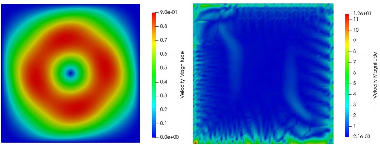
Figure 1: Velocity magnitude contours for the versatile mixed method with BDM elements of degree $k=2$ (left) and the standard DG method with $k=3$ (right) at Ma = $0.005$ and $t=0.18$.

We can see in table 3 that our mixed methods follow the expected trend, and significantly outperform the standard DG approach at low Mach numbers. In particular, we can see that around Ma = $0.01$, the DG method experiences a large spike in error, as the solution stops converging towards the incompressible results. In addition, we can see from figure 1 that while our BDM method maintains the initial decaying vortex, the DG solution has become completely unphysical. We note that the DG method does not always produce unphysical results, as it generates accurate results at some lower and higher Mach numbers, (Ma $\geq 0.05$ and Ma $\leq 0.0005$). However, generally speaking, the accuracy of the DG method in the low-Mach-number regime is unreliable. Here, we have demonstrated that it is possible for the DG method to converge to a non-physical solution in this regime. In our experience, this phenomenon was not observed for the versatile mixed methods with Taylor-Hood or BDM elements. We believe that this highlights a clear advantage of our approach: namely, since we are using function spaces traditionally associated with incompressible flows, we are successfully able to capture near-incompressible flow, even when solving the compressible equations.

5.3 2-D Cylinder in Cross Flow

For the third test case, we simulated a two-dimensional cylinder in cross flow over a range of Mach numbers, at a fixed Reynolds number Re = $100$. In particular, the simulations were run with a uniform inlet flow, where the Mach number was adjusted over the following range of values: Ma = $0.1$, $0.2$, $0.3$, and $0.4$. For these experiments, we utilized an initial density of $\rho$ = $1.0$ kg/m³. The viscosity inside of the domain was allowed to change in accordance with Sutherland’s law. The fixed Reynolds number at the inlet was maintained by adjusting the inlet viscosity in accordance with the inlet Mach number. In addition, a fixed Prandtl number Pr = $0.72$ was used. The following fluid properties were assumed: $C_{v}$ = $717.8$ J/kg-K and $\gamma$ = $1.4$. The boundary condition for the left-most boundary was a subsonic inlet condition, and for the right-most boundary it was an extrapolation condition. The top and bottom boundaries utilized symmetry boundary conditions. The cylinder itself was equipped with adiabatic no-slip walls.

The computational domain was $\Omega$ = $[-20,40]$ $\times[-20,20]$. The cylinder had a diameter of $0.1247$ m and was centered at the point $(0,0)$. We used a mesh with $70,000$ unstructured triangular elements. The polynomial order was $k=2$, and the simulations were run for $t\in[0,200]$ with a time-step of $\Delta t=$ $1.5\times 10^{-5}$. Data for post-processing purposes was sampled over $t\in[150,200]$.

For this study, the primary quantity of interest was the time-averaged drag coefficient of the cylinder, $C_{d}$, defined as

$$C_{d}=\frac{\overline{F}_{d}}{\frac{1}{2}\rho_{\infty}u_{\infty}^{2}d}.$$ (5.1)

Here, $\overline{F}_{d}$ is the time-averaged drag force acting on the cylinder, $\rho_{\infty}$ is the free-stream density, $u_{\infty}$ is the free-stream flow speed, and $d$ is the diameter of the cylinder.

In what follows, we compare our results against an earlier study performed by [79] on an identical geometry. At the given Reynolds number (100), the reference predicts that the flow will be unsteady with an oscillatory wake structure. This behavior is independent of the Mach number, as long as Ma $<0.6$. As such, the flow fields for the various Mach numbers all exhibit similar behavior, which is correctly predicted for the Ma = 0.4 case by our method, (see figure  2). In particular, we can see from the figure the previously mentioned oscillatory wake behavior with the sinusoidal streamlines leaving the cylinder. This behavior is consistent across all Mach numbers, and implies that at least qualitatively we are in agreement with the reference solution.

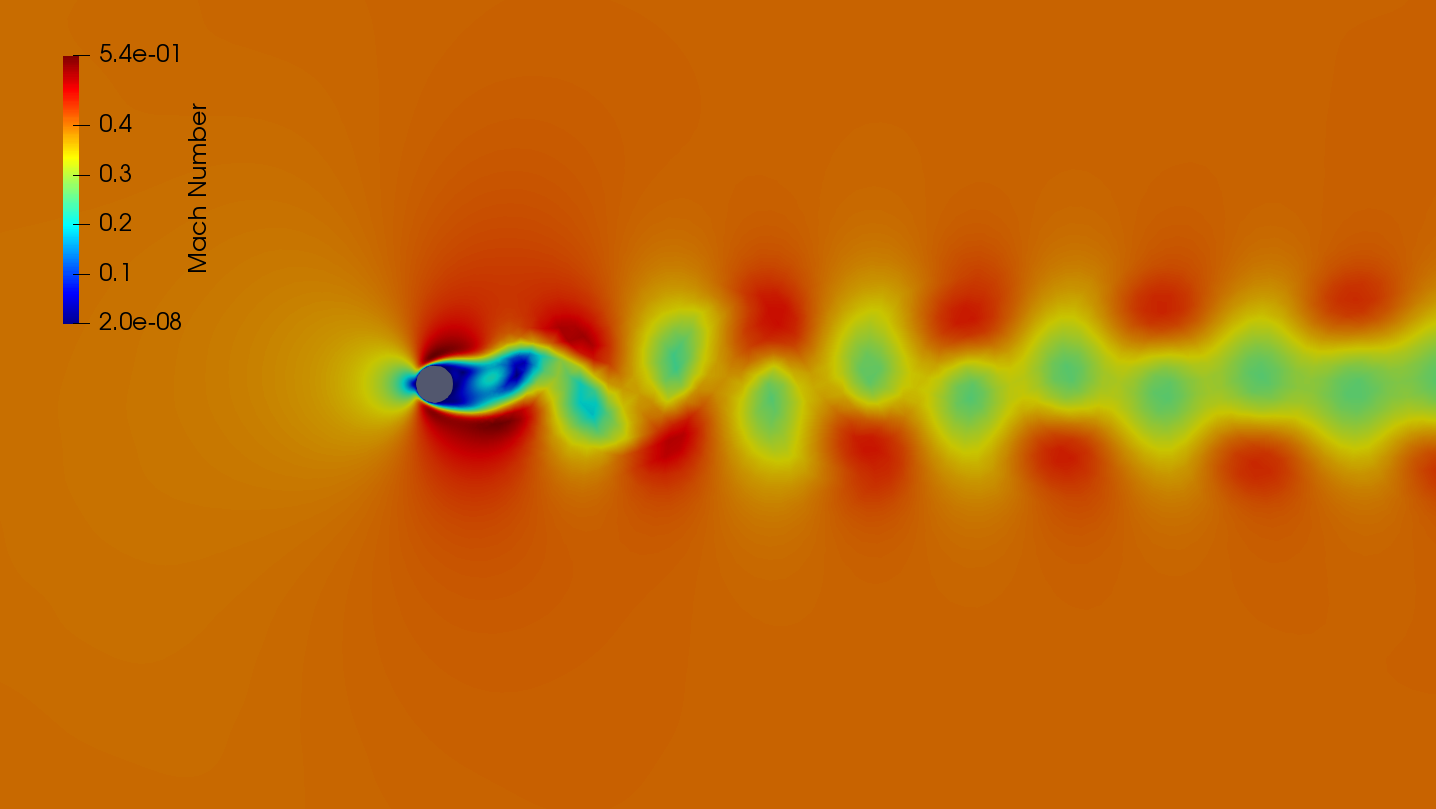
Figure 2: A snapshot of Mach number contours for the 2-D cylinder in cross flow at Ma = 0.4. Results were obtained using the versatile mixed method with Taylor-Hood elements of degree $k=2$.

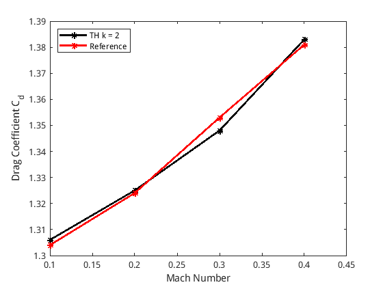
Figure 3: A plot of the time-averaged drag coefficient vs. the Mach number. Results were obtained using the versatile mixed method with Taylor-Hood elements of degree $k=2$, and the reference [79].

In figure  3, we compare our predictions for the drag coefficients with those of the reference solution [79]. The predicted drag coefficient is in good agreement with the reference across the full range of Mach numbers considered.

5.4 Joukowski Airfoil

The final test case involved flow over a Joukowski airfoil. This case was introduced at the 4th International Workshop on High-order CFD Methods, (see [80]). Here, an airfoil is simulated at an angle of attack of 0 degrees. The flow has Reynolds and Mach numbers of Re = 1000 and Ma = 0.5. The Prandtl number is again fixed at Pr = 0.72. Fluid properties for all simulations were $C_{v}=717.8$ J/kg-K, $\mu=1.716\times 10^{-5}$ kg/m-s, and $\gamma=1.4$. The viscosity was varied via Sutherland’s Law. The initial density was prescribed as $\rho$ = 1 kg/m³. The boundary conditions were specified as a subsonic inlet condition on the left-most boundary, and an extrapolation condition on the right-most boundary. The airfoil itself was equipped with an adiabatic, no-slip condition.

The domain was $\Omega$ = $[-100,100]$ $\times[-100,100]$ with the airfoil starting at $(0,0)$. The length of the airfoil from nose to trailing edge was 1 m. Unstructured meshes with 16,384, 65,536, and 262,144 triangular elements were used to tessellate the domain. These meshes were provided by organizers of the 5th International Workshop on High-order CFD Methods, and are numbered as meshes 2, 3, and 4, (see [81]). The simulations were run with polynomial order $k=2$ on these meshes until the drag converged to a steady-state value.

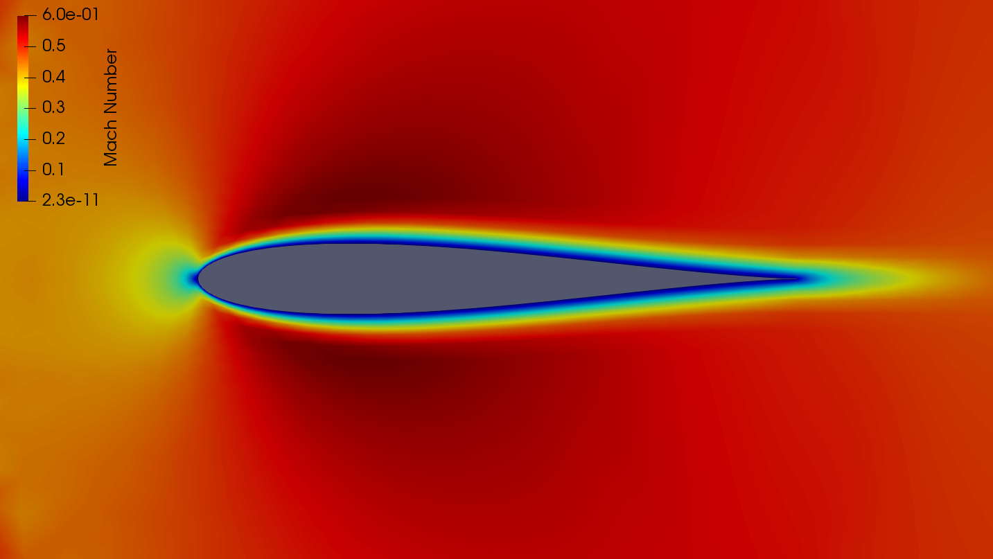
Figure 4: Mach number contours for the Joukowski airfoil at Re = $1000$ and Ma = $0.5$. Results were obtained using the versatile mixed method with Taylor-Hood elements of degree $k=2$ on the finest mesh.

DoF Count	$C_{d}$
16,704	0.1320
66,176	0.1273
263,424	0.1221

Table 4: A table of drag coefficients on the given meshes. Results were obtained using the versatile mixed method with Taylor-Hood elements of degree $k=2$. The reference value for this case is $C_{d}=0.1219$

Our results on mesh 4 are shown in figure 4. Here, the flow around the airfoil appears to be laminar, and the wake coming off the trailing edge has reached a steady state.

The primary challenge for this case is to converge to the reference drag coefficient using the meshes provided. In table 4, we see that, as we increase the degrees of freedom in the simulation, we move closer to the reference steady-state value of $C_{d}=0.1219$. On the final grid, there is reasonable agreement between our predicted value and the reference.

6 Conclusion

In this work, we introduce a new class of ‘versatile mixed finite element methods’ for solving the compressible Navier-Stokes equations. These methods appear to be unique, as they simultaneously leverage multiple stabilization strategies for solving problems in the incompressible and compressible flow regimes. More precisely, our methods leverage numerical-flux-based stabilization, kinetic-energy-based stabilization, and inf-sup-based stabilization strategies.

We note that our philosophy for designing these methods is somewhat unusual. In particular, many numerical methods are only designed to be stable for linear advection and diffusion problems. In contrast, we have created finite element methods which are provably stable for the non-linear, non-isothermal, incompressible Navier-Stokes equations. Therefore, the starting point for our methods is significantly more complex than most, which facilitates their robustness and flexibility, in terms of successful application to increasingly complex problems. This claim has been demonstrated within the present paper, where we have successfully extended our methods to solve weakly- and fully-compressible flows.

The proposed methods are primarily designed to maintain their performance in the incompressible limit. In fact, we have ensured that the methods are ‘incompressibly stable’, which means they are mathematically guaranteed to maintain stability when the density, dynamic viscosity coefficient, and heat conductivity coefficient assume constant values. We have shown through numerical experiments, that the resulting methods maintain good convergence properties and stability as the Mach number approaches zero. Based on this evidence, we argue that most (if not all) methods designed for weakly-compressible flows should satisfy the ‘incompressible stability’ property.

Lastly, we note that the new methods perform well, even far away from the incompressible limit, for flows in which the local Mach number exceeds 0.5. Of course, our numerical experiments in this regard are not exhaustive. Therefore, subsequent work will be needed to investigate the properties of these methods at higher Mach numbers (and Reynolds numbers), in an effort to establish their validity in these more challenging contexts.

Declaration of Competing Interests

The authors declare that they have no known competing financial interests or personal relationships that could have appeared to influence the work reported in this paper.

Funding

This research did not receive any specific grant from funding agencies in the public, commercial, or not-for-profit sectors.

Appendix A Derivation of the Finite Element Methods

A.1 Mass Equation Derivation

One may substitute $\rho_{h}$ and $\bm{u}_{h}$ into Eq. (2.1), multiply by a test function $q_{h}$, and integrate over the entire domain in order to yield

$$\left(\partial_{t}\,\rho_{h},q_{h}\right)_{\mathcal{T}_{h}}+\left(\nabla_{h}\cdot\left(\rho_{h}\bm{u}_{h}\right),q_{h}\right)_{\mathcal{T}_{h}}=\left(S_{\rho},q_{h}\right)_{\mathcal{T}_{h}}.$$ (A.1)

This is identical to Eq. (3.1).

A.2 Linear Momentum Equation Derivation

One may substitute $\rho_{h}$, $\bm{u}_{h}$, and $T_{h}$ into Eq. (2.2), compute the dot product with a test function $\bm{w}_{h}$, and integrate over the entire domain in order to yield

$$\left(\partial_{t}\left(\rho_{h}\bm{u}_{h}\right),\bm{w}_{h}\right)_{\mathcal{T}_{h}}+\left(\nabla_{h}\cdot\left(\left(\rho_{h}\bm{u}_{h}\right)\otimes\bm{u}_{h}+P_{h}\mathbb{I}\right),\bm{w}_{h}\right)_{\mathcal{T}_{h}}-\left(\nabla_{h}\cdot\left(\rho_{h}\bm{\tau}_{h}\right),\bm{w}_{h}\right)_{\mathcal{T}_{h}}=\left(\bm{S}_{u},\bm{w}_{h}\right)_{\mathcal{T}_{h}}.$$ (A.2)

Upon integrating the second and third terms on the LHS by parts and inserting numerical fluxes $\widehat{\bm{\sigma}}_{\text{inv}}$ and $\widehat{\bm{\sigma}}_{\text{vis}}$, one obtains

$$\left(\nabla_{h}\cdot\left(\left(\rho_{h}\bm{u}_{h}\right)\otimes\bm{u}_{h}+P_{h}\mathbb{I}\right),\bm{w}_{h}\right)_{\mathcal{T}_{h}}$$ (A.3)

$$=-\left(\left(\rho_{h}\bm{u}_{h}\right)\otimes\bm{u}_{h}+P_{h}\mathbb{I},\nabla_{h}\bm{w}_{h}\right)_{\mathcal{T}_{h}}+\left\langle\left(\left(\rho_{h}\bm{u}_{h}\right)\otimes\bm{u}_{h}+P_{h}\mathbb{I}\right)\bm{n},\bm{w}_{h}\right\rangle_{\partial\mathcal{T}_{h}}$$

$$\equiv-\left(\left(\rho_{h}\bm{u}_{h}\right)\otimes\bm{u}_{h}+P_{h}\mathbb{I},\nabla_{h}\bm{w}_{h}\right)_{\mathcal{T}_{h}}+\left\langle\widehat{\bm{\sigma}}_{\text{inv}}\,\bm{n},\bm{w}_{h}\right\rangle_{\partial\mathcal{T}_{h}}$$

$$=-\left(\left(\rho_{h}\bm{u}_{h}\right)\otimes\bm{u}_{h},\nabla_{h}\bm{w}_{h}\right)_{\mathcal{T}_{h}}-\left(P_{h},\nabla\cdot\bm{w}_{h}\right)_{\mathcal{T}_{h}}+\left\langle\widehat{\bm{\sigma}}_{\text{inv}}\,\bm{n},\bm{w}_{h}\right\rangle_{\partial\mathcal{T}_{h}}.$$

$$-\left(\nabla_{h}\cdot\left(\rho_{h}\bm{\tau}_{h}\right),\bm{w}_{h}\right)_{\mathcal{T}_{h}} =\left(\rho_{h}\bm{\tau}_{h},\nabla_{h}\bm{w}_{h}\right)_{\mathcal{T}_{h}}-\left\langle\rho_{h}\bm{\tau}_{h}\,\bm{n},\bm{w}_{h}\right\rangle_{\partial\mathcal{T}_{h}}$$ (A.4)

$$\equiv\left(\rho_{h}\bm{\tau}_{h},\nabla_{h}\bm{w}_{h}\right)_{\mathcal{T}_{h}}-\left\langle\widehat{\bm{\sigma}}_{\text{vis}}\,\bm{n},\bm{w}_{h}\right\rangle_{\partial\mathcal{T}_{h}}.$$

Consider substituting the definition of $\bm{\tau}_{h}$ (Eq. (2.8)) into the first term on the RHS of Eq. (A.4)

$$\left(\rho_{h}\bm{\tau}_{h},\nabla_{h}\bm{w}_{h}\right)_{\mathcal{T}_{h}}=\left(\mu_{h}\left(\nabla_{h}\bm{u}_{h}+\nabla_{h}\bm{u}_{h}^{T}-\frac{2}{3}\left(\nabla\cdot\bm{u}_{h}\right)\mathbb{I}\right),\nabla_{h}\bm{w}_{h}\right)_{\mathcal{T}_{h}}.$$ (A.5)

One may expand each term in Eq. (A.5) by integrating by parts, inserting a numerical flux $\widehat{\bm{\varphi}}_{\text{vis}}$, and integrating by parts again as follows

$$\left(\mu_{h}\nabla_{h}\bm{u}_{h},\nabla_{h}\bm{w}_{h}\right)_{\mathcal{T}_{h}} =\left(\nabla_{h}\bm{u}_{h},\mu_{h}\nabla_{h}\bm{w}_{h}\right)_{\mathcal{T}_{h}}$$ (A.6)

$$=-\left(\bm{u}_{h},\nabla_{h}\cdot\left(\mu_{h}\nabla_{h}\bm{w}_{h}\right)\right)_{\mathcal{T}_{h}}+\left\langle\mu_{h}\bm{u}_{h},\left(\nabla_{h}\bm{w}_{h}\right)\bm{n}\right\rangle_{\partial\mathcal{T}_{h}}$$

$$\equiv-\left(\bm{u}_{h},\nabla_{h}\cdot\left(\mu_{h}\nabla_{h}\bm{w}_{h}\right)\right)_{\mathcal{T}_{h}}+\left\langle\widehat{\bm{\varphi}}_{\text{vis}},\left(\nabla_{h}\bm{w}_{h}\right)\bm{n}\right\rangle_{\partial\mathcal{T}_{h}}$$

$$=\left(\mu_{h}\nabla_{h}\bm{u}_{h},\nabla_{h}\bm{w}_{h}\right)_{\mathcal{T}_{h}}+\left\langle\widehat{\bm{\varphi}}_{\text{vis}}-\mu_{h}\bm{u}_{h},\left(\nabla_{h}\bm{w}_{h}\right)\bm{n}\right\rangle_{\partial\mathcal{T}_{h}}.$$

$$\left(\mu_{h}\nabla_{h}\bm{u}_{h}^{T},\nabla_{h}\bm{w}_{h}\right)_{\mathcal{T}_{h}} =\left(\nabla_{h}\bm{u}_{h},\mu_{h}\nabla_{h}\bm{w}_{h}^{T}\right)_{\mathcal{T}_{h}}$$ (A.7)

$$=-\left(\bm{u}_{h},\nabla_{h}\cdot\left(\mu_{h}\nabla_{h}\bm{w}_{h}^{T}\right)\right)_{\mathcal{T}_{h}}+\left\langle\mu_{h}\bm{u}_{h},\left(\nabla_{h}\bm{w}_{h}^{T}\right)\bm{n}\right\rangle_{\partial\mathcal{T}_{h}}$$

$$\equiv-\left(\bm{u}_{h},\nabla_{h}\cdot\left(\mu_{h}\nabla_{h}\bm{w}_{h}^{T}\right)\right)_{\mathcal{T}_{h}}+\left\langle\widehat{\bm{\varphi}}_{\text{vis}},\left(\nabla_{h}\bm{w}_{h}^{T}\right)\bm{n}\right\rangle_{\partial\mathcal{T}_{h}}$$

$$=\left(\mu_{h}\nabla_{h}\bm{u}_{h}^{T},\nabla_{h}\bm{w}_{h}\right)_{\mathcal{T}_{h}}+\left\langle\widehat{\bm{\varphi}}_{\text{vis}}-\mu_{h}\bm{u}_{h},\left(\nabla_{h}\bm{w}_{h}^{T}\right)\bm{n}\right\rangle_{\partial\mathcal{T}_{h}}.$$

$$\left(-\frac{2}{3}\mu_{h}\left(\nabla\cdot\bm{u}_{h}\right)\mathbb{I},\nabla_{h}\bm{w}_{h}\right)_{\mathcal{T}_{h}} =-\frac{2}{3}\left(\left(\nabla\cdot\bm{u}_{h}\right),\mu_{h}\nabla\cdot\bm{w}_{h}\right)_{\mathcal{T}_{h}}$$ (A.8)

$$=-\frac{2}{3}\left(-\left(\bm{u}_{h},\nabla_{h}\left(\mu_{h}\nabla_{h}\cdot\bm{w}_{h}\right)\right)_{\mathcal{T}_{h}}+\left\langle\mu_{h}\bm{u}_{h},\left(\nabla\cdot\bm{w}_{h}\right)\bm{n}\right\rangle_{\partial\mathcal{T}_{h}}\right)$$

$$\equiv-\frac{2}{3}\left(-\left(\bm{u}_{h},\nabla_{h}\left(\mu_{h}\nabla_{h}\cdot\bm{w}_{h}\right)\right)_{\mathcal{T}_{h}}+\left\langle\widehat{\bm{\varphi}}_{\text{vis}},\left(\nabla\cdot\bm{w}_{h}\right)\bm{n}\right\rangle_{\partial\mathcal{T}_{h}}\right)$$

$$=\left(-\frac{2}{3}\mu_{h}\left(\nabla\cdot\bm{u}_{h}\right)\mathbb{I},\nabla_{h}\bm{w}_{h}\right)_{\mathcal{T}_{h}}-\frac{2}{3}\left\langle\widehat{\bm{\varphi}}_{\text{vis}}-\mu_{h}\bm{u}_{h},\left(\nabla\cdot\bm{w}_{h}\right)\bm{n}\right\rangle_{\partial\mathcal{T}_{h}}.$$

Upon combining Eqs. (A.6) – (A.8) along with the definition of $\bm{\tau}_{h}$ (Eq. (2.8)), one obtains

$$\left(\rho_{h}\bm{\tau}_{h},\nabla_{h}\bm{w}_{h}\right)_{\mathcal{T}_{h}}\equiv\left(\rho_{h}\bm{\tau}_{h},\nabla_{h}\bm{w}_{h}\right)_{\mathcal{T}_{h}}+\left\langle\widehat{\bm{\varphi}}_{\text{vis}}-\mu_{h}\bm{u}_{h},\left(\nabla_{h}\bm{w}_{h}+\nabla_{h}\bm{w}_{h}^{T}-\frac{2}{3}\left(\nabla\cdot\bm{w}_{h}\right)\mathbb{I}\right)\bm{n}\right\rangle_{\partial\mathcal{T}_{h}}.$$ (A.9)

Finally, one may substitute Eqs. (A.3), (A.4), and (A.9), into Eq. (A.2), in order to obtain Eq. (3.2).

A.3 Internal Energy Equation Derivation

One may substitute $\rho_{h}$, $\bm{u}_{h}$, and $T_{h}$ into Eq. (2.3), multiply by a test function $r_{h}$, and integrate over the entire domain in order to yield

$$\left(\partial_{t}\left(\rho_{h}T_{h}\right),r_{h}\right)_{\mathcal{T}_{h}}+\left(\nabla_{h}\cdot\left(\rho_{h}T_{h}\bm{u}_{h}\right),r_{h}\right)_{\mathcal{T}_{h}}-\left(\nabla_{h}\cdot\left(\frac{\kappa_{h}}{C_{v}}\nabla_{h}T_{h}\right),r_{h}\right)_{\mathcal{T}_{h}}$$

$$=-\left(\gamma-1\right)\left(\rho_{h}T_{h}\left(\nabla\cdot\bm{u}_{h}\right),r_{h}\right)_{\mathcal{T}_{h}}+\frac{1}{C_{v}}\left(\rho_{h}\bm{\tau_{h}}:\nabla_{h}\bm{u}_{h},r_{h}\right)_{\mathcal{T}_{h}}+\left(S_{T},r_{h}\right)_{\mathcal{T}_{h}}.$$ (A.10)

Upon integrating the second and third terms on the LHS by parts and inserting numerical fluxes $\widehat{\bm{\phi}}_{\text{inv}}$ and $\widehat{\bm{\phi}}_{\text{vis}}$, one obtains

$$\left(\nabla_{h}\cdot\left(\rho_{h}T_{h}\bm{u}_{h}\right),r_{h}\right)_{\mathcal{T}_{h}} =-\left(\rho_{h}T_{h}\bm{u}_{h},\nabla_{h}r_{h}\right)_{\mathcal{T}_{h}}+\left\langle\left(\rho_{h}T_{h}\bm{u}_{h}\right)\cdot\bm{n},r_{h}\right\rangle_{\partial\mathcal{T}_{h}}$$ (A.11)

$$\equiv-\left(\rho_{h}T_{h}\bm{u}_{h},\nabla_{h}r_{h}\right)_{\mathcal{T}_{h}}+\left\langle\widehat{\bm{\phi}}_{\text{inv}}\cdot\bm{n},r_{h}\right\rangle_{\partial\mathcal{T}_{h}}.$$

$$-\left(\nabla_{h}\cdot\left(\frac{\kappa_{h}}{C_{v}}\nabla_{h}T_{h}\right),r_{h}\right)_{\mathcal{T}_{h}} =\left(\frac{\kappa_{h}}{C_{v}}\nabla_{h}T_{h},\nabla_{h}r_{h}\right)_{\mathcal{T}_{h}}-\left\langle\left(\frac{\kappa_{h}}{C_{v}}\nabla_{h}T_{h}\right)\cdot\bm{n},r_{h}\right\rangle_{\partial\mathcal{T}_{h}}$$ (A.12)

$$\equiv\left(\frac{\kappa_{h}}{C_{v}}\nabla_{h}T_{h},\nabla_{h}r_{h}\right)_{\mathcal{T}_{h}}-\left\langle\widehat{\bm{\phi}}_{\text{vis}}\cdot\bm{n},r_{h}\right\rangle_{\partial\mathcal{T}_{h}}.$$

One may further expand Eq. (A.12). Consider integrating by parts, inserting the numerical flux $\widehat{\lambda}_{\text{vis}}$, and integrating by parts again as follows

$$\left(\nabla_{h}T_{h},\frac{\kappa_{h}}{C_{v}}\nabla_{h}r_{h}\right)_{\mathcal{T}_{h}} =-\left(T_{h},\nabla_{h}\cdot\left(\frac{\kappa_{h}}{C_{v}}\nabla_{h}r_{h}\right)\right)_{\mathcal{T}_{h}}+\left\langle\frac{\kappa_{h}}{C_{v}}T_{h},\nabla_{h}r_{h}\cdot\bm{n}\right\rangle_{\partial\mathcal{T}_{h}}$$ (A.13)

$$\equiv-\left(T_{h},\nabla_{h}\cdot\left(\frac{\kappa_{h}}{C_{v}}\nabla_{h}r_{h}\right)\right)_{\mathcal{T}_{h}}+\left\langle\widehat{\lambda}_{\text{vis}},\nabla_{h}r_{h}\cdot\bm{n}\right\rangle_{\partial\mathcal{T}_{h}}$$

$$=\left(\frac{\kappa_{h}}{C_{v}}\nabla_{h}T_{h},\nabla_{h}r_{h}\right)_{\mathcal{T}_{h}}+\left\langle\widehat{\lambda}_{\text{vis}}-\frac{\kappa_{h}}{C_{v}}T_{h},\nabla_{h}r_{h}\cdot\bm{n}\right\rangle_{\partial\mathcal{T}_{h}}.$$

Finally, one may combine Eqs. (A.10)–(A.13) in order to obtain Eq. (3.3).

References

- [1] X. Chen, D. M. Williams, Versatile mixed methods for the incompressible Navier–Stokes equations, Computers & Mathematics with Applications 80 (6) (2020) 1555–1577.
- [2] E. A. Miller, X. Chen, D. M. Williams, Versatile mixed methods for non-isothermal incompressible flows, Computers & Mathematics with Applications 125 (2022) 150–175.
- [3] M. Mallet, A finite element method for computational fluid dynamics, Ph.D. thesis, Stanford University Stanford, CA (1985).
- [4] T. J. Hughes, M. Mallet, A new finite element formulation for computational fluid dynamics: III. the generalized streamline operator for multidimensional advective-diffusive systems, Computer Methods in Applied Mechanics and engineering 58 (3) (1986) 305–328.
- [5] F. Shakib, T. J. R. Hughes, Z. Johan, A new finite element formulation for computational fluid dynamics: X. the compressible Euler and Navier-Stokes equations, Computer Methods in Applied Mechanics and Engineering (1991) 141–219.
- [6] T. Hughes, F. Shakib, Computational aerodynamics and the finite element method, in: AIAA 25th Aerospace Sciences Meeting, Reno, Nevada, 1988.
- [7] T. J. Hughes, L. P. Franca, G. M. Hulbert, A new finite element formulation for computational fluid dynamics: VIII. the Galerkin/least-squares method for advective-diffusive equations, Computer Methods in Applied Mechanics and Engineering 73 (2) (1989) 173–189.
- [8] P. B. Bochev, M. D. Gunzburger, Least-squares finite element methods, Vol. 166, Springer Science & Business Media, 2009.
- [9] T. J. Hughes, G. R. Feijóo, L. Mazzei, J.-B. Quincy, The variational multiscale method—a paradigm for computational mechanics, Computer Methods in Applied Mechanics and Engineering 166 (1-2) (1998) 3–24.
- [10] T. J. Hughes, L. Mazzei, K. E. Jansen, Large eddy simulation and the variational multiscale method, Computing and Visualization in Science 3 (2000) 47–59.
- [11] V. John, S. Kaya, A finite element variational multiscale method for the Navier–Stokes equations, SIAM Journal on Scientific Computing 26 (5) (2005) 1485–1503.
- [12] T. J. Hughes, G. Sangalli, Variational multiscale analysis: the fine-scale Green’s function, projection, optimization, localization, and stabilized methods, SIAM Journal on Numerical Analysis 45 (2) (2007) 539–557.
- [13] B. Cockburn, C.-W. Shu, TVB Runge–Kutta local projection discontinuous Galerkin finite element method for conservation laws. II. General framework, Mathematics of Computation 52 (186) (1989) 411–435.
- [14] B. Cockburn, S.-Y. Lin, C.-W. Shu, TVB Runge–Kutta local projection discontinuous Galerkin finite element method for conservation laws III: One-dimensional systems, Journal of Computational Physics 84 (1) (1989) 90–113.
- [15] B. Cockburn, S. Hou, C.-W. Shu, The Runge–Kutta local projection discontinuous Galerkin finite element method for conservation laws. IV. The multidimensional case, Mathematics of Computation 54 (190) (1990) 545–581.
- [16] B. Cockburn, C.-W. Shu, The Runge–Kutta local projection -discontinuous Galerkin finite element method for scalar conservation laws, RAIRO-Modélisation mathématique et analyse numérique 25 (3) (1991) 337–361.
- [17] B. Cockburn, C.-W. Shu, The Runge–Kutta discontinuous Galerkin method for conservation laws V: Multidimensional systems, Journal of Computational Physics 141 (2) (1998) 199–224.
- [18] F. Bassi, S. Rebay, G. Mariotti, S. Pedinotti, M. Savini, A high-order accurate discontinuous finite element method for inviscid and viscous turbomachinery flows, in: Proceedings of the 2nd European Conference on Turbomachinery Fluid Dynamics and Thermodynamics, Technologisch Instituut, Antwerpen, Belgium, 1997, pp. 99–109.
- [19] F. Bassi, S. Rebay, High-order accurate discontinuous finite element solution of the 2D Euler equations, Journal of Computational Physics 138 (2) (1997) 251–285.
- [20] F. Bassi, S. Rebay, A high-order accurate discontinuous finite element method for the numerical solution of the compressible Navier–Stokes equations, Journal of Computational Physics 131 (2) (1997) 267–279.
- [21] J. Peraire, P.-O. Persson, The compact discontinuous Galerkin (CDG) method for elliptic problems, SIAM Journal on Scientific Computing 30 (4) (2008) 1806–1824.
- [22] S. Brdar, A. Dedner, R. Klöfkorn, Compact and stable discontinuous Galerkin methods for convection-diffusion problems, SIAM Journal on Scientific Computing 34 (1) (2012) A263–A282.
- [23] Y. Pan, P.-O. Persson, Agglomeration-based geometric multigrid solvers for compact discontinuous galerkin discretizations on unstructured meshes, Journal of Computational Physics 449 (2022) 110775.
- [24] B. Cockburn, J. Gopalakrishnan, R. Lazarov, Unified hybridization of discontinuous Galerkin, mixed, and continuous Galerkin methods for second order elliptic problems, SIAM Journal on Numerical Analysis 47 (2) (2009) 1319–1365.
- [25] P. Fernandez, N. C. Nguyen, J. Peraire, The hybridized discontinuous Galerkin method for implicit large-eddy simulation of transitional turbulent flows, Journal of Computational Physics 336 (2017) 308–329.
- [26] P. Fernández, Entropy-stable hybridized discontinuous Galerkin methods for large-eddy simulation of transitional and turbulent flows, Ph.D. thesis, Massachusetts Institute of Technology (2019).
- [27] B. Cockburn, J. Guzmán, S.-C. Soon, H. K. Stolarski, An analysis of the embedded discontinuous Galerkin method for second-order elliptic problems, SIAM Journal on Numerical Analysis 47 (4) (2009) 2686–2707.
- [28] N. C. Nguyen, J. Peraire, B. Cockburn, A class of embedded discontinuous Galerkin methods for computational fluid dynamics, Journal of Computational Physics 302 (2015) 674–692.
- [29] N. V. Roberts, L. Demkowicz, R. Moser, A discontinuous Petrov–Galerkin methodology for adaptive solutions to the incompressible Navier–Stokes equations, Journal of Computational Physics 301 (2015) 456–483.
- [30] T. Ellis, L. Demkowicz, J. Chan, Locally conservative discontinuous Petrov–Galerkin finite elements for fluid problems, Computers & Mathematics with Applications 68 (11) (2014) 1530–1549.
- [31] T. E. Ellis, Space-time discontinuous Petrov-Galerkin finite elements for transient fluid mechanics, Ph.D. thesis, University of Texas, Austin (2016).
- [32] W. Rachowicz, A. Zdunek, W. Cecot, A discontinuous Petrov-Galerkin method for compressible Navier-Stokes equations in three dimensions, Computers & Mathematics with Applications 102 (2021) 113–136.
- [33] A. C. Huang, H. A. Carson, S. R. Allmaras, M. C. Galbraith, D. L. Darmofal, D. S. Kamenetskiy, A variational multiscale method with discontinuous subscales for output-based adaptation of aerodynamic flows, in: AIAA Scitech 2020 Forum, 2020, p. 1563.
- [34] A. Huang, An adaptive variational multiscale method with discontinuous subscales for aerodynamic flows, Ph.D. thesis, Massachusetts Institute of Technology (2020).
- [35] H. A. Carson, Provably convergent anisotropic output-based adaptation for continuous finite element discretizations, Ph.D. thesis, Massachusetts Institute of Technology (2020).
- [36] T. J. Hughes, L. P. Franca, M. Mallet, A new finite element formulation for computational fluid dynamics: I. Symmetric forms of the compressible Euler and Navier-Stokes equations and the second law of thermodynamics, Computer Methods in Applied Mechanics and Engineering 54 (2) (1986) 223–234.
- [37] A. Harten, On the symmetric form of systems of conservation laws with entropy, Journal of Computational Physics 49.
- [38] E. Tadmor, Skew-self adjoint form for systems of conservation laws, Journal of Mathematical Analysis and Applications 103 (2) (1984) 428–442.
- [39] T. J. Barth, Numerical methods for gasdynamic systems on unstructured meshes, An Introduction to recent developments in theory and numerics for conservation laws. Springer Berlin Heidelberg (1999) 195–285.
- [40] T. J. Barth, On discontinuous Galerkin approximations of Boltzmann moment systems with Levermore closure, Computer Methods in Applied Mechanics and Engineering 195 (25) (2006) 3311–3330.
- [41] D. Williams, An entropy stable, hybridizable discontinuous Galerkin method for the compressible Navier-Stokes equations, Mathematics of Computation 87 (309) (2018) 95–121.
- [42] D. M. Williams, An analysis of discontinuous Galerkin methods for the compressible Euler equations: entropy and L2 stability, Numerische Mathematik 141 (4) (2019) 1079–1120.
- [43] J. Guzmán, C.-W. Shu, F. A. Sequeira, H-(div) conforming and DG methods for incompressible Euler’s equations, IMA Journal of Numerical Analysis 37 (4) (2016) 1733–1771.
- [44] G. J. Gassner, A kinetic energy preserving nodal discontinuous Galerkin spectral element method, International Journal for Numerical Methods in Fluids 76 (1) (2014) 28–50.
- [45] S. Ortleb, Kinetic energy preserving DG schemes based on summation-by-parts operators on interior node distributions, PAMM 16 (1) (2016) 857–858.
- [46] S. Ortleb, A kinetic energy preserving DG scheme based on Gauss–Legendre points, Journal of Scientific Computing 71 (2017) 1135–1168.
- [47] D. Flad, G. Gassner, On the use of kinetic energy preserving DG-schemes for large eddy simulation, Journal of Computational Physics 350 (2017) 782–795.
- [48] B. F. Klose, G. B. Jacobs, D. A. Kopriva, Assessing standard and kinetic energy conserving volume fluxes in discontinuous Galerkin formulations for marginally resolved Navier-Stokes flows, Computers & Fluids 205 (2020) 104557.
- [49] A. Jameson, The construction of discretely conservative finite volume schemes that also globally conserve energy or entropy, Journal of Scientific Computing 34 (2) (2008) 152–187.
- [50] A. Jameson, Formulation of kinetic energy preserving conservative schemes for gas dynamics and direct numerical simulation of one-dimensional viscous compressible flow in a shock tube using entropy and kinetic energy preserving schemes, Journal of Scientific Computing 34 (2008) 188–208.
- [51] Y. Allaneau, A. Jameson, Kinetic energy conserving discontinuous Galerkin scheme, in: 49th AIAA Aerospace Sciences Meeting including the New Horizons Forum and Aerospace Exposition, 2011, p. 198.
- [52] D. Boffi, F. Brezzi, M. Fortin, Mixed Finite Element Methods and Applications, Vol. 44, Springer, 2013.
- [53] V. John, Finite Element Methods for Incompressible Flow Problems, Vol. 51, Springer, 2016.
- [54] P. W. Schroeder, G. Lube, Pressure-robust analysis of divergence-free and conforming FEM for evolutionary incompressible Navier–Stokes flows, Journal of Numerical Mathematics.
- [55] P. W. Schroeder, G. Lube, Divergence-free H(div)-FEM for time-dependent incompressible flows with applications to high Reynolds number vortex dynamics, Journal of Scientific Computing (2018) 1–29.
- [56] P. W. Schroeder, C. Lehrenfeld, A. Linke, G. Lube, Towards computable flows and robust estimates for inf-sup stable FEM applied to the time-dependent incompressible Navier–Stokes equations, SeMA Journal, Boletin de la Sociedad Española de Matemática Aplicada 75 (4) (2018) 629–653.
- [57] H. Dallmann, D. Arndt, G. Lube, Local projection stabilization for the Oseen problem, IMA Journal of Numerical Analysis 36 (2) (2015) 796–823.
- [58] J. Schütz, G. May, A hybrid mixed method for the compressible Navier–Stokes equations, Journal of Computational Physics 240 (2013) 58–75.
- [59] J. Schütz, G. May, An adjoint consistency analysis for a class of hybrid mixed methods, IMA Journal of Numerical Analysis 34 (3) (2014) 1222–1239.
- [60] J. R. Kweon, Optimal error estimate for a mixed finite element method for compressible Navier–Stokes system, Applied Numerical Mathematics 45 (2-3) (2003) 275–292.
- [61] R. B. Kellogg, B. Liu, A finite element method for the compressible Stokes equations, SIAM Journal on Numerical Analysis 33 (2) (1996) 780–788.
- [62] L. Zhang, Z. Chen, et al., A stabilized mixed finite element method for single-phase compressible flow, Journal of Applied Mathematics 2011.
- [63] H. Egger, A robust conservative mixed finite element method for isentropic compressible flow on pipe networks, SIAM Journal on Scientific Computing 40 (1) (2018) A108–A129.
- [64] Y.-H. Choi, C. L. Merkle, The application of preconditioning in viscous flows, Journal of Computational Physics 105 (2) (1993) 207–223.
- [65] E. Turkel, Review of preconditioning methods for fluid dynamics, Applied Numerical Mathematics 12 (1-3) (1993) 257–284.
- [66] D. Lee, B. Van Leer, Progress in local preconditioning of the Euler and Navier-Stokes equations, in: 11th Computational Fluid Dynamics Conference, 1993, p. 3328.
- [67] J. M. Weiss, W. A. Smith, Preconditioning applied to variable and constant density flows, AIAA Journal 33 (11) (1995) 2050–2057.
- [68] E. Turkel, Preconditioning techniques in computational fluid dynamics, Annual Review of Fluid Mechanics 31 (1) (1999) 385–416.
- [69] H. Guillard, C. Viozat, On the behaviour of upwind schemes in the low Mach number limit, Computers & Fluids 28 (1) (1999) 63–86.
- [70] A. Meister, Asymptotic based preconditioning technique for low Mach number flows, ZAMM-Journal of Applied Mathematics and Mechanics/Zeitschrift für Angewandte Mathematik und Mechanik: Applied Mathematics and Mechanics 83 (1) (2003) 3–25.
- [71] P. Birken, A. Meister, Stability of preconditioned finite volume schemes at low Mach numbers, BIT Numerical Mathematics 45 (3) (2005) 463–480.
- [72] P. Birken, A. Meister, On low Mach number preconditioning of finite volume schemes, PAMM: Proceedings in Applied Mathematics and Mechanics 5 (1) (2005) 759–760.
- [73] P.-O. Persson, J. Peraire, Newton-GMRES preconditioning for discontinuous Galerkin discretizations of the Navier–Stokes equations, SIAM Journal on Scientific Computing 30 (6) (2008) 2709–2733.
- [74] F. Bassi, C. De Bartolo, R. Hartmann, A. Nigro, A discontinuous Galerkin method for inviscid low Mach number flows, Journal of Computational Physics 228 (11) (2009) 3996–4011.
- [75] A. Nigro, C. De Bartolo, R. Hartmann, F. Bassi, Discontinuous Galerkin solution of preconditioned euler equations for very low Mach number flows, International Journal for Numerical Methods in Fluids 63 (4) (2010) 449–467.
- [76] B. Klein, B. Müller, F. Kummer, M. Oberlack, A high-order discontinuous Galerkin solver for low Mach number flows, International Journal for Numerical Methods in Fluids 81 (8) (2016) 489–520.
- [77] A. Gouasmi, S. M. Murman, K. Duraisamy, Entropy-stable schemes in the low-Mach-number regime: Flux-preconditioning, entropy breakdowns, and entropy transfers, Journal of Computational Physics 456 (2022) 111036.
- [78] M. S. Alnaes, J. Blechta, J. Hake, A. Johansson, B. Kehlet, A. Logg, C. Richardson, J. Ring, M. E. Rognes, G. N. Wells, The FEniCS project version 1.5, Archive of Numerical Software 3 (100) (2015) 9–23.
- [79] D. Canuto, K. Taira, Two-dimensional compressible viscous flow around a circular cylinder, Journal of Fluid Mechanics 785 (2015) 349–371.
- [80] M. Galbraith, C. Ollivier-Gooch, 4th International Workshop on High-Order Methods. Laminar Joukowski airfoil at Re=1000, https://how4.cenaero.be/sites/how4.cenaero.be.
- [81] M. Galbraith, 5th International Workshop on High-Order Methods. Laminar Joukowski airfoil at Re=1000, https://how5.cenaero.be/sites/how5.cenaero.be.