Quantifying Human Priors over Social and Navigation Networks
Abstract
Human knowledge is largely implicit and relational — do we have a friend in common? can I walk from here to there? In this work, we leverage the combinatorial structure of graphs to quantify human priors over such relational data. Our experiments focus on two domains that have been continuously relevant over evolutionary timescales: social interaction and spatial navigation. We find that some features of the inferred priors are remarkably consistent, such as the tendency for sparsity as a function of graph size. Other features are domain-specific, such as the propensity for triadic closure in social interactions. More broadly, our work demonstrates how nonclassical statistical analysis of indirect behavioral experiments can be used to efficiently model latent biases in the data.
1 Brains Rely on Efficient Priors
A foundational result in the fields of artificial intelligence, neuroscience, and psychology is the establishing of the central role played by inductive biases or priors in learning (Shiffrin et al., 2020; Wolpert, 2021). The importance of priors cannot be understated; indeed, their quantification elucidates many aspects of our perception and cognition.
The efficient coding hypothesis. Examples of how priors inform neuroscience can often be understood through the lens of the “efficient coding hypothesis”, which states that neural representations have adapted to efficiently encode the relevant statistics of our environment (Barlow et al., 1961).
Several decades of work investigating and refining this hypothesis have contributed to major advances in our understanding of the neural code (Manookin & Rieke, 2023). For example, many properties of mammalian visual cells (such as sensitivity to orientation and spatial frequency) have been shown to be optimized for transmitting information about natural scenes (Simoncelli, 2003; Field, 1989).
Likewise, the mammalian cochlea and auditory nerve fibers have properties that allow for efficient representation of the acoustic structure of speech and other natural sounds (Lewicki, 2002; McDermott et al., 2013). Other computations, such as visual attention (Orbán et al., 2008) and working memory (Mathy & Feldman, 2012; Brady et al., 2009), display analogous properties.
Visual priors color our perception. This principle of efficient coding also explains several well-known visual illusions (Howe & Purves, 2005; Howe et al., 2005), evidentiating a general and important computational tradeoff in biology: priors cannot be both exhaustive and efficient. That is, by efficiently distinguishing relevant visual information, our priors render us blind to insignificant differences. Might there be similar “illusions” with respect to our priors over the structure of connections?
2 Tasks are Often Relational
From roads between places, websites on the internet, words in a text, and friendships between people, humans are routinely confronted with a web of things (nodes) structured in terms of their relations (edges). Despite the pervasiveness of networks in our lives, knowledge of our priors about them is rather sparse.
However, one notable paradigm is the learning of network structure from random walks (Lynn & Bassett, 2020; Klishin & Bassett, 2022). This approach typically consists of showing nodes to participants in a temporal sequence that respects the structure of the network (such as samples of random walks), and comparing the ease with which they learn these transitions for several different networks (Schapiro et al., 2013; Tompson et al., 2019).
Complementing these detailed experiments on specific networks, our work focuses on quantifying humans’ initial beliefs about all such networks. The motivating question is: given a set of things and minimal or no information about how they relate, what is the prior likelihood assigned to each of the many possible patterns of connections?
Why we focus on navigation and social networks. Tasks related to spatial navigation and social interaction have been quotidian over evolutionary timescales. Thus, our brains have likely adapted to efficiently encode them. Indeed, there is much evidence supporting this hypothesis. For example, the hippocampus encodes a spatial map of the environment (Maguire et al., 2003; Eichenbaum, 2017). Likewise, there are brain regions specialized in the processing of social information and theory of mind (i.e., the modeling of others’ mental states) (Richardson, 2019; Devaine et al., 2014).
Additionally, these two domains are qualitatively different: spatial navigation networks are constrained by physical space, whereas social networks are more abstract and interconnected. Comparing the similarities and differences of our priors in these domains could aid in building a more complete understanding of their associated neural processes.
3 Overview of our Framework
The number of unique configurations of connections between nodes grows superexponentially111For a feeling for the scaling, see table 3 (appendix B.2). (Sloane, 1964). This poses several difficulties in quantifying human priors over such graphs:
-
1.
engaging human attention in experiments that involve reasoning about such a large number of possibilities;
-
2.
properly sampling the space of graphs; and
-
3.
meaningfully summarizing and comparing priors over such a high-dimensional space.
We now provide a brief overview of how our framework overcomes these challenges, expanding on the details in the subsequent sections.
3.1 Engaging Human Attention
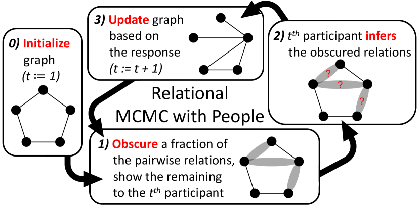
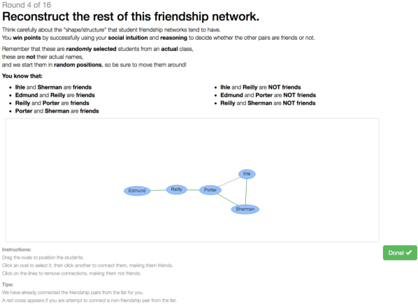
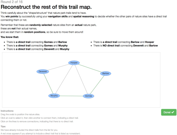
We built an online experimental platform that allowed participants to easily draw their inferences about obscured relations in a graph (demo video and fig. 1). In brief, participants were shown “partial graphs”, containing all the nodes, but only some of the pairwise relations between them, and were then asked to infer the existence (or absence) of the remaining relations. The meaning of these graphs was given by one of the four cover stories that served as the context for our experiments (table 1).
Deploying this platform in MTurk (Amazon Web Services, 2010), we carefully curated a large amount of human data in experiments involving social and spatial navigation networks (over participants and data points). To ensure that the final design was as engaging and intuitive as possible, we ran a variety of pilot experiments (over participants). This effort paid off: for the final experiments, the post-questionnaire feedback was quite positive (several MTurk workers even sent personal emails about how enjoyable the “game” was!), and the data were of high quality (see appendix A.4 for details).
obscured relations between pairs of nodes in a context.
| domain | context | nodes | relations |
|---|---|---|---|
| social | class | students | friendships |
| work | coworkers | friendships | |
| navigation | city | neighborhoods | borders |
| park | nature sites | trails |


Our online platform allowed participants to easily “draw” their inferences about the obscured relations of a graph (demo video). Note that the two images above are nearly identical: to make the comparisons as fair as possible, we made the experiments identical in every aspect, except for the text specifically related to each cover story. See appendix A for a detailed description of these experiments and high-resolution versions of these images (figs. 7 class and 8 park).
3.2 Sampling the Space of Graphs
For the first participants, we initialized our experiments using graphs spanning a wide range of edge densities. From these, we generated partial graphs, and asked participants to infer the remaining relations. We then repeatedly used the responses from the previous participants to generate partial graphs for the next participants (fig. 2). In essence, our online platform instantiates a “Markov Chain Monte Carlo algorithm with People (MCMCP)”, with multiple chains being built in parallel.
Standard implementations of MCMCP experiments model the (shared) prior of the participants by sampling (some of) their responses from (sufficiently long) experimental chains. Here, we use the data more efficiently (figs. 12 and 13) by leveraging the graphical structure to fit the aggregated responses of participants to a natural Bayesian model (section 5.2). In particular, we parameterize their priors using a hierarchical family of maximum entropy distributions over graphs (sections 5.3 and 5.4), which offer “smooth”222In the sense that graphs that differ by fewer edges are assigned similar probabilities. low-dimensional parameterizations of the high-dimensional space of graphs (figs. 14 and 15).
3.3 Summarizing and Interpreting Priors over Graphs
Graph cumulants (Bravo-Hermsdorff et al., 2021; Gunderson & Bravo-Hermsdorff, 2020) capture what is typically meant by “substructure” or “motif”: a subgraph whose prevalence in a distribution over graphs is statistically different from that which would be expected due to the prevalence of smaller subgraphs contained in . Here, we compare the inferred priors using the scaled version of graph cumulants, which additionally takes into account the density of connections (figs. 4 and 5).
4 Experimental Design
In this section, we provide a brief overview of the literature on MCMC with People (sections 4.1.1 and 4.1.2), the general framework to which our method can be applied. We then describe our experiments (sections 4.1.3 and 4.2).
4.1 Markov Chain Monte Carlo with People (MCMCP)
4.1.1 Related Work
Iterated learning refers to the process whereby a participant learns from data generated by another participant, who themselves learned it the same way, and so on. It is a highly-researched and ubiquitous psychological phenomenon — language and cultural evolution being two important examples (Kirby et al., 2014; Morgan et al., 2020). Under some assumptions (see appendix D), iterated learning can be modelled as a Markov Chain Monte Carlo algorithm instantiated by the Participants (algorithm 1) that has as its stationary distribution their shared prior over the relevant space (Griffiths & Kalish, 2007).
This MCMCP model has been employed to quantify human priors in a variety of contexts, such as: locations in visual scenes (Langlois et al., 2021); variations in facial features (Uddenberg & Scholl, 2018); strengths of causal relationships (Yeung & Griffiths, 2015); moral categories of words in ethics (Hsu et al., 2019); names of colors (Xu et al., 2013); and kernels for Gaussian processes (Schulz et al., 2017). This framework has also been applied to quantify priors of (non-human) large language models (Yamakoshi et al., 2022; Marjieh et al., 2022).
4.1.2 The MCMCP Model
Let be the space of all combinations of participants might be given in the experiment. And let be the space of all that the participants might consider when giving their responses. We assume that both spaces are discrete and finite, and denote the space of probability distributions over them as and , respectively.
The Experimentalist uses the of the previous participant (i.e., their response) to generate noisy/partial to give to the next participant. This process is a probabilistic map from , denoted in algorithm 1 as Expmnt, with associated probability distribution .
Given a prior distribution , and presented with , a “Bayesian” Participant will sample a from their posterior distribution as their response:
This process is a probabilistic map from , and is denoted in algorithm 1 as Ptcpnt.
If all participants have a shared prior distribution over the , the composition of these stochastic maps has this prior as its unique stationary distribution (given the standard technical conditions on the Markov chain, see appendix D.1).
4.1.3 Relational MCMCP
Figure 2 illustrates our algorithm for generating MCMCP experiments on graphs. It consists of the following steps:
-
0.
Initialize the chain with a graph containing nodes and pairwise relations between them (e.g., the friendships, or lack thereof, between students in a class).
-
1.
Obscure a random fraction of this graph’s pairwise relations (e.g., in fig. 2).
-
2.
Based on this “partial graph”, ask the participant to infer the obscured relations.
-
3.
Update the graph based on their response.
-
4.
Repeat the sequence of steps 1, 2, and 3, each time with a new participant.
Our experiments focused on simple graphs: undirected unweighted graphs with no self-loops or parallel edges.333So, a simple graph with nodes has pairwise relations.
For a given chain of our experiment, the space of is , the set of simple graphs with nodes, and denotes the response of the participant in the iteration/round. The space of is , the set of all partial graphs with nodes and of the pairwise relations obscured, and denotes the specific partial graph shown to the participant in the iteration/round. The map takes a graph on nodes, and makes a partial graph by randomly obscuring pairwise relations.
4.2 Experimental Platform and Cover Stories
We developed an online experimental platform and recruited participants using MTurk. Our platform allows participants to easily draw their inferences about the obscured relations in the graph (demo video) and allocates them to one of multiple experimental chains in real time. Each experiment had one of four different cover stories: two in the social domain and two in the navigation domain (table 1).
In a given experiment, a participant gave responses for many rounds, where each round was part of a different chain. A response was included in a chain (and thereby used to generate the partial graph for the next participant) only if it passed judiciously-chosen criteria. In appendix A, we provide a more detailed description of the experiments, the data collection, and the data cleaning procedures.
The experiment begins with an introduction about the particular cover story and poses several questions to the participant to ensure their understanding. After a video demonstration of the interactive platform, each round begins with the partial graph at the center of the interactive interface and a list of the “unobscured” relations at the top of the screen. Using this interface, the participant were able to move the nodes and add/remove edges (fig. 1).
Once the participant submitted their response, a question appears about which node(s) they thought to be the most/least important (asked in a variety of ways). To incentivize participants to respond using their true prior, they were told during the introduction that there is a ground truth and they would be rewarded for correctly guessing the relations that were obscured (see appendix A.5 for the complete text). Clearly, as there is not such a ground truth, their responses did not influence their final payoff (though their level of engagement did, see appendix A.4).
As the analysis assumes that the nodes are exchangeable, we aimed to make their labels as neutral as possible. To this end, we randomly selected the node labels from a long list of last names, while ensuring that no name was repeated during an experiment. Participants were clearly instructed that the node labels were fictitious names, and that they provided no information about the “correct” answers.
5 Data Analysis
In this section, we describe how we analyze the data from our experiments. We first discuss how data from MCMCP experiments is typically used to obtain priors and some of the limitations of this standard approach. We then introduce our method, which alleviates these issues by exploiting the Bayesian assumption (section 5.2), and uses the combinatorial structure of graphs to fit the data with a natural family of maximum entropy models (sections 5.3, and 5.4). We end this section by describing how we quantify and compare relevant characteristics of the inferred priors (sections 5.5, 5.6, and 5.7).
5.1 Limitations of the Standard MCMCP Approach
Typically, studies employing MCMCP experiments use the participants’ responses towards the end of the chains as a proxy for their prior. Indeed, according to the assumptions of the MCMCP model, the stationary distribution of (Bayesian) participants’ responses approximates their (shared) prior over the relevant .
However, this approach wastes much of the collected data for two reasons. First, one must discard the initial responses until the chain has (hopefully444Determining convergence can be highly nontrivial in certain cases, especially when the state space is large (Roy, 2020).) converged (sufficiently close555This can also be nontrivial to determine.) to its stationary distribution, the so-called “burn-in” period (Raftery & Lewis, 1996). Second, as the responses are correlated, one cannot treat them as completely independent samples, and thus has fewer effective samples (Hsu et al., 2015). Moreover, the number of iterations/rounds required for an experimental chain to be sufficiently close to its stationary distribution (i.e., its mixing time) is highly dependent on the probabilistic mapping used to generate the experiments, and on the participants’ (unknown) prior (see figs. 10 and 11).
While this might not always be a problem (such as when samples can be efficiently generated by a computer), using human participants to generate samples in MCMCP often presents a significant bottleneck (controlling electrons is typically simpler than controlling human attention).
5.2 Leveraging the Bayesian Ansatz
Instead of using (a few of) the observed responses to approximate the prior, we exploit the fact that the paired data are more informative than these alone. Specifically, as the traditional approach already assumes that the participants are Bayesian with the same prior, we make explicit use of this implicit assumption by modelling the paired data in terms of the transition matrix induced by an underlying shared prior . In appendix E.1, we show that this fitting approach alleviates typical problems of standard MCMCP data analysis: estimating the mixing time (fig. 12) and correlated samples (fig. 13).
An important hurdle still remains: for this fitting approach to work, one must be able to parameterize the priors. However, as mentioned in section 3, the number of nonisomorphic graphs grows superexponentially in their number of nodes . It is thus unwise to fit a multinomial distribution to each of these graphs, thereby, effectively treating them as incomparable variables. To obtain informative priors, we must use a meaningful low-dimensional smooth parameterization of probability distributions over graphs, such that graphs that differ by fewer edges are given similar probabilities.
We now describe a natural hierarchical family of network models that provides such a parameterization (section 5.3) and how we fit these models to the data (section 5.4). In appendix E.2, we show that this choice of parameterization for the priors leads to a more accurate recovery of the prior in simulated data (where the ground truth is known) (fig. 14) and improved generalization in real data (fig. 15).
5.3 Modeling the Priors using a Hierarchy of
Maximum Entropy Distributions over Graphs
Intuitively, given a set of constraints, the maximum entropy distribution is the “simplest” of those that satisfy the constraints (Jaynes, 1957a, b). Maximum entropy distributions appear in every corner of science; from uniform to Gaussian, beta to binomial, gamma to Poisson and more, nearly all named distributions maximize entropy in some sense.
For simple graphs with nodes, the simplest statistic is the edge density . The maximum entropy distribution corresponding to this statistic is the Erdős–Rényi model , in which a connection appears between each of the pairs of the nodes independently with the same probability . In particular, the distribution assigns uniform probability to each of the graphs with labeled nodes, and serves as the base measure for any maximum entropy distribution over simple graphs with nodes (node-labeled or not).
These distributions are known as Exponential Random Graphs Models (ERGMs). They have been extensively studied theoretically (Chatterjee & Diaconis, 2013; Cimini et al., 2019) and applied to a wide range of real networks (Lusher et al., 2013; Lehmann et al., 2021). Although it is possible to define an ERGM by prescribing any set of realizable constraints, a natural and frequent choice (Lovász, 2012; Lauritzen et al., 2018) is to prescribe the counts/densities of small subgraphs, such as edges (), “cherries” (), and triangles ().
To model the priors, we use the following family of ERGMs:
| (1) |
where is a simple graph with nodes; is a distribution over such graphs; is the (injective homomorphism666 Consider all injective maps (so no node overlapping) from the nodes of into the nodes of , is the fraction of such maps for which every edge in appears in the corresponding location in (i.e., we do not care about the absence of edges).) density of the subgraph in the graph ; is the parameter associated with ; and are all subgraphs with at most edges.
That is, this model constrains the densities of all subgraphs with at most edges (hence the sum over ). This choice induces a natural and convenient hierarchy of network models for the priors. In particular, the parameter controls the expressivity of the model. For example, constrains only the edge density , corresponding to the simplest network model . Likewise, constrains the density of all subgraphs with edges, leading to a far more complex model for the prior (e.g., this model can exactly specify the probability of all graphs with nodes).
5.4 Fitting and Selecting the Model
When fitting a model to the prior, we consider all data related to a particular cover story and a given number of nodes. Specifically, we aggregate data from all such chains regardless of fraction of relations obscured , as when we split the data, there were no significant differences.
For each subgraph in the model (eq. 1), there is a corresponding (conjugate) parameter . We fit these parameters numerically by maximizing the log-likelihood of the data:
where denotes the participant’s response to being shown the partial graph ; and the distribution is that which would be obtained by including edges i.i.d. with probability for each of the obscured relationships in .777Indeed, this is how participants would reply if their prior were (corresponding to ).
We employed Newton’s method to obtain the parameters for which , and selected the model complexity using cross-validation and various sanity checks and robustness tests (see appendix B.1).
5.5 Interpreting the Data using Graph Cumulants
Just as the classical cumulants (e.g., mean, variance, covariance, skew, kurtosis) can be derived from the classical moments, so too can graph cumulants be obtained from the subgraph densities (the analogue of moments for graphs Bickel et al. (2011)). Graph cumulants are a principled and intuitive family of subgraph-based statistics that naturally captures the propensity (or aversiveness) for any substructure of interest (see Bravo-Hermsdorff et al. (2021) for a concise application or Gunderson & Bravo-Hermsdorff (2020) for more details).
Intuitively, the graph cumulant quantifies the difference between the observed density of subgraph and the density that would be expected by chance due to the densities of smaller subgraphs within . For example, for the cherry cumulant , a term involving the edge density is subtracted from the cherry density: . For , terms involving both the edge and cherry densities, and , are subtracted. For the simplest random graph , which has no graphical structure beyond the presence of edges, all graph cumulants (aside from 888Just as the mean is the first moment and the first cumulant, the edge density is likewise the first graph moment and the first graph cumulant .) are exactly zero, reflecting the fact that larger subgraphs do not require more explanation than just the edge density.
5.6 Scaling the Graph Cumulants Accounts for Sparsity
If one randomly deletes edges i.i.d. in a graph such that a fraction of the edges remain, then the resulting expected edge density is clearly scaled by a factor of from the original edge density. Similarly, for a subgraph with edges, its expected subgraph density and graph cumulant are scaled by a factor of . This can make comparisons between subgraphs of different sizes difficult, especially for sparse graph distributions. As such, we report the scaled graph cumulants (i.e., ) of the inferred priors.
5.7 Estimating the Error in our Results
The solid curves in figures 3, 4, and 5 display (scaled) graph cumulants of the inferred priors. To estimate our uncertainty in these measurements, we simulated ideal Bayesian MCMCP agents using the inferred priors, and responding to the same partial graphs seen by the participants. We then inferred the prior for each of these synthetic datasets, and computed their (scaled) graph cumulants. The shaded regions correspond to standard deviation about the average of these values (for repetitions of this process).
6 Results
While our analysis of participants’ data makes full use of the MCMCP assumptions (most notably, that participants are Bayesian with the same prior), we are not claiming that they exactly hold in practice. Nevertheless, the results we present below are remarkably robust (as evidenced by model selection, sensitivity analysis, and robustness checks), suggesting that the general conclusions are still meaningful.
6.1 Substructures with Noticeable Trends in the Priors
We now present the results for: edge density (fig. 3), scaled cherry cumulant (fig. 4), and scaled triangle cumulant (fig. 5) for each of the four cover stories as a function of the number of nodes in the prior.999Despite number of nodes clearly being a discrete variable, we plot the results as curves to aid in the visualization of the trends.
Intuitively, these statistics quantify well-known tendencies of real networks: sparsity, degree heterogeneity, and clustering, respectively. It is perhaps then not a coincidence that the subgraphs associated with these statistics were those that displayed the most discernible trends across the priors.
Priors favor sparsity. As shown in figure 3, we find that the edge density () systematically decreases as the number of nodes increases. The number of connections per node, however, appears to be a slowly increasing function of the number of nodes. This result is remarkably similar for all the four different cover stories.
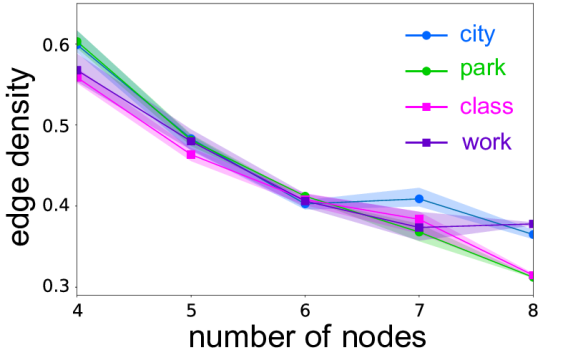
Markers in the solid curves correspond to the inferred edge density () of participants’ priors, using the aggregated data of a single cover story with that number of nodes. Shading corresponds to standard deviation of the average value that would have been obtained if participants all had this inferred prior, and behaved according to the assumptions of the MCMCP model. Note that the result of this procedure is not necessarily centered around the empirical values (i.e., the solid curves).
Priors favor uniform degrees in small graphs. As shown in figure 4, we find that the preference for degree heterogeneity (i.e., a few “hub” nodes with many of connections) increases as the number of nodes increases. The scaled cherry cumulant () changes from negative (for graphs with or nodes) to positive (for graphs with or more nodes). This suggests that human priors for small graphs favor a notably uniform distribution of node degrees, switching to a preference for heterogeneous node degrees for larger graphs. Again, this result is remarkably consistent for all four cover stories.
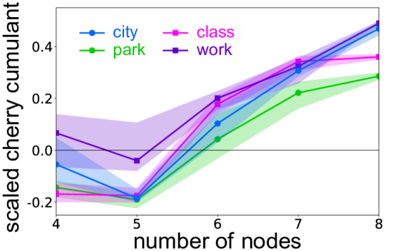
The analysis is the same as in fig. 3, but the statistic measured is the scaled cherry cumulant (), which quantifies preference for degree heterogeneity. A negative value indicates that the prior has edges distributed more uniformly than what would be expected by chance (i.e., in an distribution with the same number of nodes and edge density ).
Priors over social interactions favor triangles. As shown in figure 5, the scaled triangle cumulant () reveals that the priors for the social domain have a notably higher preference for clustering.101010For measuring clustering in bipartite graphs, one should use the scaled square cumulant . In contrast to the edge () and cherry (), this motif () clearly distinguishes between the social and navigation domains.
Indeed, Tompson et al. (2019) found experimental evidence that humans learn community structure differently when the network is social vs. non-social. Moreover, the prevalence of triadic closure in social networks (i.e., one’s friends tend to be friends with each other) is a well-established phenomenon (Yang et al., 2016).
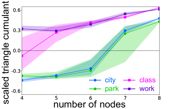
The analysis is the same as in figs. 3 and 4, but the statistic measured is the scaled triangle cumulant (), which quantifies preference for clustering. A negative value indicates that the prior has fewer triangles than what would be expected by chance. In contrast to figs. 3 and 4, there is a notable difference between the social (class and work) and navigation (city and park) domains.
6.2 Generalization Between and Within Domains
In figure 6, we compare generalization within domain and between domains. In particular, for a given number of nodes and model expressivity (equation 1) for the priors, we randomly partitioned the data from each of the cover stories into a training set () and a test set (). Then, for each of the combinations of cover stories, we fit the (order ) model to the training data and measured the average log-likelihood per round (which we denote by “avgLL”) of the test data under this model. To compare to a meaningful baseline, we subtracted the avgLL of this test data under a “non-specialized” model that was fit to the combined training data of all four cover stories.
The decimal numbers shown in figure 6 are the exponential of these differences in avgLL, having “units” of a ratio of probabilities. A value of corresponds to the specialized model explaining the data equally as well as the non-specialized model, while a value greater than one indicates that the specialized model explains the data better than the non-specialized model (and conversely for a value less than one). Figure 6 shows the average result for repetitions of this procedure.
Larger subgraphs reveal differences between domains. As a general trend, we find that more complex models recover priors that are better able to differentiate between domains and (to a lesser degree) specific cover stories. This is reflected in figure 6 by the suggestively “block-diagonal” appearance of the -by- squares corresponding to more expressive models (). The “horizontal-row” appearance of the -by- squares corresponding to suggests that the quality of fit for less complex models is determined primarily by the particular data used for testing. These results are in agreement with our previous findings that larger motifs (and triangles in particular) are needed in order to distinguish between the two domains (figs. 3, 4, and 5).
A note on planar graphs. One aspect worth mentioning is the duality between our two spatial navigation cover stories. While both are suggestively planar, their connectivity is of two different flavors. The trails in the park cover story are rather analogous to vectors (a “large” trail implies a large separation between the two nature sites), while the boundaries between neighborhoods in the city cover story are analogous to one-forms (a “large” boundary between neighborhoods implies that they are nearby). While in our results, the similarity between the priors for these two navigation cover stories is about the same as the similarity between those for the two social cover stories, it is possible that future investigations involving weighted graphs could reflect this difference.
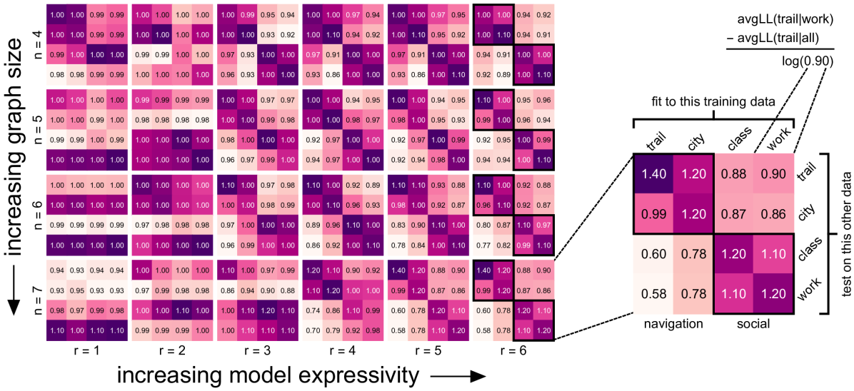
The -by- layout divides the results by the number of nodes (rows) and the model complexity (columns) of the priors. Each of these options for and contains results summarized by a -by- square of numbers. For each of these -by- square, we fit “specialized” models (using the training data of each cover story separately), as well as one “non-specialized” model (using the combined training data of all cover stories). As seen in the amplified -by- square on the right, the columns denote the cover story of the specialized training data, and the rows denote the cover story of the test data used to evaluate these models. The numbers inside these squares are defined in section 6.2 and rounded to the nearest . They can be approximately thought of as an average odds-ratio; a value of corresponds to the case when the specialized model assigns a probability to an actual response of a participant that is about times the probability assigned by the non-specialized model. The coloring of the squares is purely for visualization; we scale the same range of colors to that square’s maximum and minimum values. While the less expressive models (to the left) are in fact much more similar than the colors suggest, the more expressive models recover priors that are better able to differentiate between domains and (to a lesser degree) specific cover stories.
7 Possible Sequels
Other structures. In addition to weighted graphs, other extensions are also possible. For example, one could investigate priors over bipartite graphs representing people’s preferences over a set of items, or priors over directed graphs modeling patterns of citations. More generally, any such MCMCP experiment might benefit from our approach of inferring the prior by explicitly fitting the assumed Bayesian model to the aggregated data.
Adaptive sampling. As our method explicitly uses the MCMCP assumptions to fit the data, there is no longer a need to collect data in chains. In fact, one could use the current fit of the prior to inform an adaptive sampling algorithm to select the presented in each iteration. As a simple example, we found that it was helpful to initialize many chains over a large range of edge densities. It is entirely possible that a similar “spreading out” over other features (like degree heterogeneity and clustering) would likewise be helpful.
Larger graphs. Our results suggest that properties of the priors vary with the number of nodes. The results presented in the main text consider graphs with at most nodes. Unfortunately, in practice, our experiments appeared to lose human engagement for graphs with or more nodes (see discussion in appendix B.2 and C, and fig. 9 for analysis of these data). Adapting our methods to measure graphs over a range of sizes would be particularly interesting, as we could compare the resulting priors with actual structure of analogous real networks. The scaled graph cumulants we used in our analysis are well-suited for such comparisons.
Different cultures. It is important to note that if we are to claim that a prior is representative of general characteristics of human cognition, it should be representative of the full diversity of the humans. In this direction, we have an ongoing collaboration with a linguist that works with the Yawanawá and the Xinane aboriginal tribes in the Amazon rainforest (Camargo Souza, 2020). In the domain of navigation, it would be interesting to see if their priors change when the discussion is about paths versus when the discussion is about regions. Results from the social domain may also prove interesting; in both tribes, while parallel-cousins (i.e., their parents are same-sex siblings) are forbidden from marriage, marriage between cross-cousins (i.e., their parents are opposite-sex siblings) is considered ideal. Case studies such as this could offer insight into the effects of community size and social norms on our priors over social networks.
General message. This paper offers a case-study about the power of carefully constructed experiments and clever analysis. Just as neural networks benefit from having architecture that reflects the symmetry of the data (Villar et al., 2023), so too does the design and analysis of experiments that use people as substrate. The results presented here demonstrate two such examples: how the assumed Bayesian structure of the participants’ responses can be used to more efficiently use the collected data, and how the relabelling symmetry of relational data can be leveraged to design more computationally tractable models for their priors.
Acknowledgements
I did this work as part of my PhD thesis at the Princeton Neuroscience Institute (PNI). I acknowledge PNI for the financial support during my PhD and the Princeton’s Cognitive Science Department for an independent research grant. The completion of this work is inextricably connected to the discussions and support shared with me by many incredible people along the PhD journey (see my acknowledgments in Bravo-Hermsdorff (2020)). Here, I would like to particularly thank: Tom Griffiths; Talmo Pereira, for his essential role in building such an amazing online game platform; and Lee M. Gunderson, whose insights and feedback permeate every bit of this work.
References
- Amazon Web Services (2010) Amazon Web Services, A. Amazon Mechanical Turk crowdsourcing website, 2010. URL mturk.com.
- Barlow et al. (1961) Barlow, H. B. et al. Possible principles underlying the transformation of sensory messages. Sensory Communication, 1:217–234, 1961.
- Bartlett (1932) Bartlett, F. C. Remembering: A study in experimental and social psychology. Cambridge University Press, 1932.
- Bayes (1763) Bayes, T. An essay towards solving a problem in the doctrine of chances. Philosophical Transactions, 53:370–418, 1763.
- Bhui & Gershman (2018) Bhui, R. and Gershman, S. J. Decision by sampling implements efficient coding of psychoeconomic functions. Psychological Review, 125(6):985, 2018.
- Bickel et al. (2011) Bickel, P. J., Chen, A., and Levina, E. The method of moments and degree distributions for network models. The Annals of Statistics, 39(5):2280–2301, 2011.
- Botvinick et al. (2015) Botvinick, M., Weinstein, A., Solway, A., and Barto, A. Reinforcement learning, efficient coding, and the statistics of natural tasks. Current Opinion in Behavioral Sciences, 5:71–77, 2015.
- Brady et al. (2009) Brady, T. F., Konkle, T., and Alvarez, G. A. Compression in visual working memory: Using statistical regularities to form more efficient memory representations. Journal of Experimental Psychology, 138:487–502, 2009.
- Bravo-Hermsdorff (2020) Bravo-Hermsdorff, G. Quantifying Human Priors over Abstract Relational Structures. PhD thesis, Princeton University, 2020.
- Bravo-Hermsdorff et al. (2021) Bravo-Hermsdorff, G., Gunderson, L. M., Maugis, P.-A., and Priebe, C. E. Quantifying network similarity using graph cumulants. arXiv:2107.11403, 2021.
- Camargo Souza (2020) Camargo Souza, L. Switch-reference as anaphora: A modular account. PhD thesis, Rutgers University, 2020.
- Canini et al. (2014) Canini, K. R., Griffiths, T. L., Vanpaemel, W., and Kalish, M. L. Revealing human inductive biases for category learning by simulating cultural transmission. Psychonomic Bulletin & Review, 21(3):785–793, 2014.
- Chatterjee & Diaconis (2013) Chatterjee, S. and Diaconis, P. Estimating and understanding exponential random graph models. The Annals of Statistics, 41(5):2428–2461, Oct 2013.
- Chazelle & Wang (2016) Chazelle, B. and Wang, C. Self-sustaining iterated learning. arXiv:1609.03960, 2016.
- Chazelle & Wang (2019) Chazelle, B. and Wang, C. Iterated learning in dynamic social networks. Journal of Machine Learning Research, 20(1):979–1006, 2019.
- Cimini et al. (2019) Cimini, G., Squartini, T., Saracco, F., Garlaschelli, D., Gabrielli, A., and Caldarelli, G. The statistical physics of real-world networks. Nature Reviews Physics, 1(1):58, 2019.
- Crowston (2012) Crowston, K. Amazon mechanical turk: A research tool for organizations and information systems scholars. In Shaping the future of ICT research: Methods and approaches, pp. 210–221. Springer, 2012.
- Deutsch (2011) Deutsch, D. The beginning of infinity: Explanations that transform the world. Penguin Books UK, 2011.
- Devaine et al. (2014) Devaine, M., Hollard, G., and Daunizeau, J. The social bayesian brain: Does mentalizing make a difference when we learn? PLoS Computational Biology, 10(12):e1003992, 2014.
- Doya et al. (2007) Doya, K., Ishii, S., Pouget, A., and Rao, R. P. Bayesian brain: Probabilistic approaches to neural coding. MIT press, 2007.
- Eichenbaum (2017) Eichenbaum, H. The role of the hippocampus in navigation is memory. Journal of Neurophysiology, 117(4):1785–1796, 2017.
- Field (1989) Field, D. J. What the statistics of natural images tell us about visual coding. Human Vision, Visual Processing, and Digital Display, 1077:269–276, 1989.
- Frydman & Jin (2022) Frydman, C. and Jin, L. J. Efficient coding and risky choice. The Quarterly Journal of Economics, 137(1):161–213, 2022.
- Griffiths & Kalish (2007) Griffiths, T. L. and Kalish, M. L. Language evolution by iterated learning with bayesian agents. Cognitive Science, 31(3):441–480, 2007.
- Gunderson & Bravo-Hermsdorff (2020) Gunderson, L. M. and Bravo-Hermsdorff, G. Introducing graph cumulants: What is the variance of your social network? arXiv:2002.03959, 2020.
- Harrison et al. (2020) Harrison, P., Marjieh, R., Adolfi, F., van Rijn, P., Anglada-Tort, M., Tchernichovski, O., Larrouy-Maestri, P., and Jacoby, N. Gibbs sampling with people. Neural Information Processing Systems (NeurIPS), 34, 2020.
- Howe & Purves (2005) Howe, C. and Purves, D. The Müller–Lyer illusion explained by the statistics of image–source relationships. Proceedings of the National Academy of Sciences, 102(4):1234–1239, 2005.
- Howe et al. (2005) Howe, C., Yang, Z., and Purves, D. The Poggendorff illusion explained by natural scene geometry. Proceedings of the National Academy of Sciences, 102(21):7707–7712, 2005.
- Hsu et al. (2019) Hsu, A. S., Martin, J. B., Sanborn, A. N., and Griffiths, T. L. Identifying category representations for complex stimuli using discrete Markov chain Monte Carlo with people. Behavior Research Methods, 2019.
- Hsu et al. (2015) Hsu, D. J., Kontorovich, A., and Szepesvári, C. Mixing time estimation in reversible Markov chains from a single sample path. Neural Information Processing Systems (NIPS), 29, 2015.
- Hu (2011) Hu, Y. Algorithms for visualizing large networks. Combinatorial Scientific Computing, 5(3):180–186, 2011.
- Huang & Rao (2011) Huang, Y. and Rao, R. P. Predictive coding. Wiley Interdisciplinary Reviews: Cognitive Science, 2(5):580–593, 2011.
- Jaynes (1957a) Jaynes, E. T. Information theory and statistical mechanics. Physical Review, 106(4):620–630, 1957a.
- Jaynes (1957b) Jaynes, E. T. Information theory and statistical mechanics. ii. Physical Review, 108(2):171–190, 1957b.
- Kirby et al. (2014) Kirby, S., Griffiths, T., and Smith, K. Iterated learning and the evolution of language. Current Opinion in Neurobiology, 28:108–114, 2014.
- Klishin & Bassett (2022) Klishin, A. A. and Bassett, D. S. Exposure theory for learning complex networks with random walks. Journal of Complex Networks, 10(5):cnac029, 2022.
- Lake et al. (2017) Lake, B. M., Ullman, T. D., Tenenbaum, J. B., and Gershman, S. J. Building machines that learn and think like people. Behavioral and Brain Sciences, 40:e253, 2017.
- Langlois et al. (2021) Langlois, T. A., Jacoby, N., Suchow, J. W., and Griffiths, T. L. Serial reproduction reveals the geometry of visuospatial representations. Proceedings of the National Academy of Sciences, 118(13), 2021.
- Lauritzen et al. (2018) Lauritzen, S., Rinaldo, A., and Sadeghi, K. Random networks, graphical models and exchangeability. Journal of the Royal Statistical Society: Series B (Statistical Methodology), 80(3):481–508, 2018.
- Lee & Vanpaemel (2017) Lee, M. D. and Vanpaemel, W. Determining informative priors for cognitive models. Psychonomic Bulletin & Review, 25(1):114–127, 2017.
- Lehmann et al. (2021) Lehmann, B., Henson, R., Geerligs, L., White, S., et al. Characterising group-level brain connectivity: A framework using bayesian exponential random graph models. NeuroImage, 225:117480, 2021.
- Lewicki (2002) Lewicki, M. S. Efficient coding of natural sounds. Nature Neuroscience, 5(4):356, 2002.
- Lovász (2012) Lovász, L. Large networks and graph limits, volume 60. American Mathematical Society, 2012.
- Lusher et al. (2013) Lusher, D., Koskinen, J., and Robins, G. Exponential random graph models for social networks: Theory, methods, and applications. Cambridge University Press, 2013.
- Lynn & Bassett (2020) Lynn, C. W. and Bassett, D. S. How humans learn and represent networks. Proceedings of the National Academy of Sciences, 117(47):29407–29415, 2020.
- Maguire et al. (2003) Maguire, E. A., Spiers, H. J., Good, C. D., Hartley, T., Frackowiak, R. S., and Burgess, N. Navigation expertise and the human hippocampus: A structural brain imaging analysis. Hippocampus, 13(2):250–259, 2003.
- Manookin & Rieke (2023) Manookin, M. B. and Rieke, F. Two sides of the same coin: Efficient and predictive neural coding. Annual Review of Vision Science, 9, 2023.
- Marjieh et al. (2022) Marjieh, R., Sucholutsky, I., Langlois, T. A., Jacoby, N., and Griffiths, T. L. Analyzing diffusion as serial reproduction. arXiv:2209.14821, 2022.
- Mathy & Feldman (2012) Mathy, F. and Feldman, J. What’s magic about magic numbers? Chunking and data compression in short-term memory. Cognition, 122(3):346–362, 2012.
- McDermott et al. (2013) McDermott, J. H., Schemitsch, M., and Simoncelli, E. P. Summary statistics in auditory perception. Nature Neuroscience, 16(4):493, 2013.
- Modica & Poggiolini (2012) Modica, G. and Poggiolini, L. A first course in probability and Markov Chains. John Wiley & Sons, 2012.
- Montague (2007) Montague, R. Your brain is (almost) perfect: How we make decisions. Penguin, 2007.
- Morgan et al. (2020) Morgan, T. J., Suchow, J. W., and Griffiths, T. L. Experimental evolutionary simulations of learning, memory and life history. Philosophical Transactions of the Royal Society B, 375(1803):20190504, 2020.
- Orbán et al. (2008) Orbán, G., Fiser, J., Aslin, R. N., and Lengyel, M. Bayesian learning of visual chunks by human observers. Proceedings of the National Academy of Sciences, 105(7):2745–2750, 2008.
- Raftery & Lewis (1996) Raftery, A. E. and Lewis, S. M. Implementing MCMC. Markov chain Monte Carlo in practice, pp. 115–130, 1996.
- Richardson (2019) Richardson, H. Development of brain networks for social functions: Confirmatory analyses in a large open source dataset. Developmental Cognitive Neuroscience, 37:100598, 2019.
- Rieke et al. (1999) Rieke, F., Warland, D., van Steveninck, R. d. R., and Bialek, W. Spikes: Exploring the Neural Code. MIT press, 1999.
- Roy (2020) Roy, V. Convergence diagnostics for Markov chain Monte Carlo. Annual Review of Statistics and Its Application, 7:387–412, 2020.
- Sanborn et al. (2018) Sanborn, S., Bourgin, D., Chang, M., and Griffiths, T. L. Representational efficiency outweighs action efficiency in human program induction. CoRR, abs/1807.07134, 2018.
- Schapiro et al. (2013) Schapiro, A. C., Rogers, T. T., Cordova, N. I., Turk-Browne, N. B., and Botvinick, M. M. Neural representations of events arise from temporal community structure. Nature Neuroscience, 16(4):486–492, 2013.
- Schulz et al. (2017) Schulz, E., Tenenbaum, J. B., Duvenaud, D., Speekenbrink, M., and Gershman, S. J. Compositional inductive biases in function learning. Cognitive Psychology, 99:44–79, 2017.
- Shiffrin et al. (2020) Shiffrin, R. M., Bassett, D. S., Kriegeskorte, N., and Tenenbaum, J. B. The brain produces mind by modeling. Proceedings of the National Academy of Sciences, 117(47):29299–29301, 2020.
- Simoncelli (2003) Simoncelli, E. P. Vision and the statistics of the visual environment. Current Opinion in Neurobiology, 13(2):144 – 149, 2003.
- Sloane (1964) Sloane, N. The online encyclopedia of integer sequences (OEIS), entry A000088, 1964. URL oeis.org/A000088.
- Thompson & Griffiths (2021) Thompson, B. and Griffiths, T. L. Human biases limit cumulative innovation. Proceedings of the Royal Society B: Biological Sciences, 288(20202752), 2021.
- Tompson et al. (2019) Tompson, S. H., Kahn, A. E., Falk, E. B., Vettel, J. M., and Bassett, D. S. Individual differences in learning social and nonsocial network structures. Journal of Experimental Psychology: Learning, Memory, and Cognition, 45(2):253, 2019.
- Uddenberg & Scholl (2018) Uddenberg, S. and Scholl, B. J. Teleface: Serial reproduction of faces reveals a whiteward bias in race memory. Journal of Experimental Psychology: General, 147(10):1466, 2018.
- Villar et al. (2023) Villar, S., Hogg, D. W., Yao, W., Kevrekidis, G. A., and Schölkopf, B. The passive symmetries of machine learning. arXiv:2301.13724, 2023.
- Wark et al. (2007) Wark, B., Lundstrom, B. N., and Fairhall, A. Sensory adaptation. Current Opinion in Neurobiology, 17(4):423–429, 2007.
- Wolpert (2021) Wolpert, D. H. What is important about the No Free Lunch theorems? In Black Box Optimization, Machine Learning, and No-Free Lunch Theorems, pp. 373–388. Springer, 2021.
- Xu et al. (2013) Xu, J., Dowman, M., and Griffiths, T. L. Cultural transmission results in convergence towards colour term universals. Proceedings of the Royal Society B: Biological Sciences, 280(20123073), 2013.
- Yamakoshi et al. (2022) Yamakoshi, T., Griffiths, T. L., and Hawkins, R. D. Probing BERT’s priors with serial reproduction chains. arXiv:2202.12226, 2022.
- Yang et al. (2016) Yang, S., Keller, F. B., and Zheng, L. Social network analysis: Methods and examples. Sage Publications, 2016.
- Yeung & Griffiths (2015) Yeung, S. and Griffiths, T. L. Identifying expectations about the strength of causal relationships. Cognitive Psychology, 76:1–29, 2015.
Appendix A Experimental Procedure
In this section, we provide a detailed description of our experiments, and protocols for data collection and cleaning.
A.1 Data Collection
All participants were recruited online using Amazon Mechanical Turk (AMT) (see e.g. Crowston (2012) for a description of the AMT system). We only recruited participants who doing our experiment for the first time and had at least of their completed “HITs” (i.e., experiments intermediated by the AMT crowdsourcing system) approved.
The experiments were approved by Princeton University’s Institutional Review Board (IRB) for human subjects, and all participants provided informed consent for the study.
The experiment lasted minutes on average and participants were paid an average wage rate of per hour.
A.2 Experimental Design
We developed a “gamified” online experimental platform that smoothly allocates participants to the appropriate experimental chains in real time.
The structure of the experiments was the same for all four cover stories (table 1). In the the two social cover stories:
-
1.
Class: participants were asked to infer the friendships (relations) between students (nodes) in a classroom (context).
-
2.
Work: participants were asked to infer the friendships (relations) between coworkers (nodes) in a workplace (context).
And in the two navigation cover stories:
-
1.
Park: participants were asked to infer the trails (relations) between nature sites (nodes) in a nature park (context).
-
2.
City: participants were asked to infer the borders (relations) between neighborhoods (nodes) in a city (context).
Each experiment began with an introduction about the particular cover story. It then posed several questions to the participant to ensure their understanding (see appendix A.5 for the full text for each of the cover stories). After that, the task/game started. It consisted of a series of “rounds”.
A round proceeded as follows (see here for a demonstration video):
-
•
Main interface page (see the screenshots in figs. 7 and 8):
In the center of the screen, there was a visualization of the graph and an interactive interface.
Using this interface, the participant could:
move the nodes, add edges to the graph, and remove edges from the graph.
The nodes were initially positioned in such a way that the nodes did not overlap and the edges were not ambiguous.111111This was achieved using a modified spring-electrical model for graph drawing (Hu, 2011), with an additional penalty for edges with the same slope. Connections that were not obscured were already placed in the graph,
along with a list of the “unobscured” relations at the top of the screen.
The most important points of the introduction for properly doing the experiment were also recalled in this page.
Once the participant was satisfied with their modifications,
they submitted their response by clicking the “Done!” button at the bottom right of the screen. -
•
Post-round engagement page:
To foster engagement, once the participant submitted their response,
a question (asked in a variety of ways) appeared about which node(s) they thought to be the most/least important.
The participant was shown the graph they had just submitted, and gave an answer
by clicking on the node(s) they thought were the most/least important before clicking the “Submit” button.
There were rounds in total in an experiment, i.e., a participant (potentially)121212See appendix A.4 for the exclusion criteria we used to decide whether to append a response to a chain. contributed to different chains, thus completing different graphs. However, a participant could, of course, quit the experiment at any point. In such cases, we still had their data up to that point recorded and we compensated the participant for the work they had completed.
These rounds consisted of rounds for each number of nodes with a varying number of relations shown (i.e., the number of relations that were not obscured out of the total number of pairwise relations ).
In particular, for each cover story, participants were randomly assigned to one of the following six options for the precise sequence of rounds:
-
1.
: , , , , , , , , , , , , , , , ;
-
2.
: , , , , , , , , , , , , , , , ;
-
3.
: , , , , , , , , , , , , , , , ;
-
4.
: , , , , , , , , , , , , , , , ;
-
5.
: , , , , , , , , , , , , , , , ; or
-
6.
: , , , , , , , , , , , , , , , .
We added participants to the chains until they contained participants. When needed, we initialized a new chain with a new random graph, sampled in a way that ensured that the initial graphs covered a large range of edge densities. Only responses that passed our exclusion criteria (described in appendix A.4) were appended to the chain.
For each of the cover stories, we ran the experiments at least until we obtained two chains of length for all the pairs in each of the six different sequences.131313For some of the chains over graphs with nodes, it took quite a few rounds of participants to obtain a response. While there are no results for graphs with , , and nodes in the main text (for reasons discussed in appendix B.2), we were able to model the density of connections for these larger graphs (as described in appendix C).
A.3 Design Considerations
We performed a variety of pilot experiments (totaling more than participants), which provided valuable insight into how to make these experiments engaging and intuitive.
For example, the first version had no visual interface for manipulating the graphs, and the participants had to remember the relations while responding to a series of yes/no questions. As our experiments are not particularly concerned about short-term memory, removing this unnecessary and cognitively taxing obstacle proved very helpful. We also added an extra question after each graph to make it more engaging, as well as many embellishments to the cover stories.
These and other improvements were incorporated into the final experiments, resulting in remarkably positive feedback in the post-experiment questionnaire, as well as several MTurk workers sending personal emails about how they found the experiments engaging.
These pilot experiments also allowed us to devise quantitative heuristics to clean the data (appendix A.4), thus (hopefully) only including “genuine” responses to the chains.
A.4 Exclusion Criteria
Data from behavioral experiments with humans, particularly when collected online, can be “contaminated” by participants that are not sufficiently engaged with the experiment. Thus, we implemented a systematic method for excluding such data from the chains. We also use this method for rewarding participants that clearly gave thoughtful deliberation to our experiments.
Our exclusion heuristics were judiciously chosen after observing the distribution of participants’ responses to our pilot experiments. Specifically, we exclude all rounds that met any of the following criteria:
-
1.
Answered too quickly:
if the participant took less than seconds per shown relation to submit their response. -
2.
Not enough interaction:
if the participant moved fewer than nodes. -
3.
Changed too little:
if and ,
where is the number of relations obscured, is the fraction of obscured relations that the participant choose to be edges in their response, and is the number of nodes. -
4.
Not enough practice:
if the participant had fewer than valid rounds.
The total number of rounds and the total number of participants for each cover story before and after the exclusion criteria are displayed in table 2.
After applying the exclusion criteria, we used approximately of the total number of data points (i.e., rounds).
| cover story | # participants: after out of total (% excluded) | # rounds: after out of total (% excluded) |
|---|---|---|
| class | out of () | out of () |
| work | out of () | out of () |
| park | out of () | out of () |
| city | out of () | out of () |
A.5 Detailed Instructions
In this section, we provide the entire instruction text, page by page, for each of the four cover stories. The instructions were broken in several pages, and participants could navigate to the next page or the previous page.
A.5.1 General Format
All experiments started with the same welcome page:
Thank you and welcome to our experiment!
Next, we will show you a few instructions.
Please read them carefully,
as you will have to correctly answer
a few questions before moving on to the game!
After the instructions, we asked participants three multiple choice questions to verify that they understood the task. Each question appeared on a single page, and participants were only allowed to move to the next page once they had answered the question correctly. If they answered correctly, they would simply see a message displaying:
Correct!
If they answered incorrectly, they would see a “wrong answer message page” with a summary of the cover story they were participating in. This message was the same for the three questions (but, of course, different for each cover story).
For all cover stories, the correct answer for the first question was option , for the second question was option , and for the third question was option .
We now provide the text specific to each cover story.
A.5.2 Cover Story: Class
Instructions
Page :
We are studying how gossip spreads in schools.
In a variety of different classes,
we recorded the friendships between pairs of students.We are testing how well people intuit these friendship networks
based on partial information.
Page :
In each class:
Some pairs of students are friends.
So, gossip can be directly transferred between these two students
without needing to pass through another student.Other pairs of students are not friends.
So, for gossip to be transferred from one to the other,
it has to pass through at least one other student.You will play the following game:
We tell you whether some pairs of students are friends or not.
Your goal is to reconstruct the rest of their friendship network.
You win points by matching the “shape/structure” of the unknown relations!
Page :
For each round of the game,
we randomly select students from the same class,
and display some of their relations at the top of the screen.For example:
- •
“Hassen and Hernandez are friends”
- •
“Miller and Fleming are NOT friends”
But the list is incomplete!
You need to use your social intuition and reasoning to
decide whether the other pairs are friends or not.You will do this by drawing the rest of their friendship network
using our graphical interface.
Page :
How to draw the friendship network:
[Here we had a quick video with a demo of the interface]
- •
To change the location of a student, click and drag their name.
- •
To connect two students, first click on one, then on the other.
A line will appear between them, indicating that they are friends.- •
To disconnect two students,
simply click on the line that connects them.
The line will disappear, indicating that they are not friends.Notes:
If there is no line between two students,
it means you think they are not friends.
Even if in your drawing they look very close to each other!
So, if you think two students are friends,
always make sure to connect them with a line.To make your job easier,
we have already connected the friendship pairs from the list for you.
And if you attempt to connect a non-friendship pair from the list,
we indicate the error with a red “X”.We start the students at random positions,
so make sure to move the students around,
as this will help you visualize the network.
Page :
Some important information:
- •
You will play this game for several rounds,
each time with a different class.- •
In each round, the students are randomly selected from the same class.
- •
The friendships were recorded from actual classrooms,
so to protect the students’ identities, we use fictitious names.
Thus, the names do not provide any information
and you should not use them to guide your answers.- •
To motivate you to do your best,
you will be paid according to your performance, which is determined by
how well your drawings match the actual friendship networks.- •
Precisely, we will keep a score for each round:
You win points for correctly inferring if
the pairs of students not presented in the list are friends or not.
You lose points if your drawing does not respect
the relations given in the list, which you know for sure are correct.
The closer you match the actual friendship networks,
the larger your bonus will be.
We will give your total score and the resulting performance bonus
only at the end of the experiment.- •
We will give you a chance to take a break at the end of each round.
Please attempt to solve each round uninterrupted.
Questions after instructions
Wrong answer message:
Sorry, but…
We recorded the friendships between pairs of students,
and we are testing how well people intuit these friendship networks
based on partial information.In particular, for each round,
we randomly select some students from the same class,
and tell you whether some pairs of students are friends or not.Your goal is to reconstruct the rest of their friendship network.
Page for question :
Before we move on,
please answer a few quick questions to make sure you understand the game.
Feel free to use the Previous button if you need to review the instructions.Here’s an easy one to get started:
What are we asking you to draw?
- 1.
Power grid networks.
- 2.
Student friendship networks.
Page for question :
What do you know about the relations between students?
- 1.
Some pairs of students are friends,
meaning gossip can transfer directly between them.
Other pairs are not friends,
so gossip must pass through at least one other student to get between them.- 2.
Some pairs of students are in the same class,
meaning they know each other.
Other pairs of students are in different classes,
which means they likely do not know each other.- 3.
Some pairs of students are in the same school,
meaning they possibly know each other.
Other pairs of individuals are in different schools,
which means they do not know each other.
Page for question :
What is your goal, and what are its main challenges?
- 1.
Your goal is to discover which classes are dysfunctional,
and therefore more likely to support bullying and bad behavior.
The main challenge is that you do not know who these students are
or the schools they come from.- 2.
Your goal is to reconstruct the friendship network
of randomly selected students.
The main challenge is that we only tell you
whether some pairs of students are friends or not.
Final instruction page:
Awesome job! You are now ready to reconstruct your first friendship network!
A.5.3 Cover Story: Work
Instructions
Page :
We are studying how gossip spreads in workplaces.
In a variety of different workplaces,
we recorded the friendships between pairs of coworkers.We are testing how well people intuit these friendship networks
based on partial information.
Page :
In each workplace:
Some pairs of coworkers are friends.
So, gossip can be directly transferred between these two coworkers
without needing to pass through another coworker.Other pairs of coworkers are not friends.
So, for gossip to be transferred from one to the other,
it has to pass through at least one other coworker.You will play the following game:
We tell you whether some pairs of coworkers are friends or not.
Your goal is to reconstruct the rest of their friendship network.
You win points by matching the “shape/structure” of the unknown relations!
Page :
For each round of the game,
we randomly select coworkers from a single workplace,
and display some of their relations at the top of the screen.For example:
- •
“Hassen and Hernandez are friends”
- •
“Miller and Fleming are NOT friends”
But the list is incomplete!
You need to use your social intuition and reasoning to
decide whether the other pairs are friends or not.You will do this by drawing the rest of their friendship network
using our graphical interface.
Page :
How to draw the friendship network:
[Here we had a quick video with a demo of the interface]
- •
To change the location of a person, click and drag their name.
- •
To connect two coworkers, first click on one, then on the other.
A line will appear between them, indicating that they are friends.- •
To disconnect two coworkers,
simply click on the line that connects them.
The line will disappear, indicating that they are not friends.Notes:
If there is no line between two coworkers,
it means you think they are not friends.
Even if in your drawing they look very close to each other!
So, if you think two coworkers are friends,
always make sure to connect them with a line.To make your job easier,
we have already connected the friendship pairs from the list for you.
And if you attempt to connect a non-friendship pair from the list,
we indicate the error with a red “X”.We start the coworkers at random positions,
so make sure to move them around,
as this will help you visualize the network.
Page :
Some important information:
- •
You will play this game for several rounds,
each time with a different workplace.- •
In each round, the coworkers are randomly selected from a single workplace.
- •
The friendships were recorded from actual workplaces,
so to protect their identities, we use fictitious names.
Thus, the names do not provide any information
and you should not use them to guide your answers.- •
To motivate you to do your best,
you will be paid according to your performance, which is determined by
how well your drawings match the actual friendship networks.- •
Precisely, we will keep a score for each round:
You win points for correctly inferring if
the pairs of coworkers not presented in the list are friends or not.
You lose points if your drawing does not respect
the relations given in the list, which you know for sure are correct.
The closer you match the actual friendship networks,
the larger your bonus will be.
We will give your total score and the resulting performance bonus
only at the end of the experiment.- •
We will give you a chance to take a break at the end of each round.
Please attempt to solve each round uninterrupted.
Questions after instructions
Wrong answer message:
Sorry, but…
We recorded the friendships between pairs of coworkers,
and we are testing how well people intuit these friendship networks
based on partial information.In particular, for each round,
we randomly select some people from a single workplace,
and tell you whether some pairs of coworkers are friends or not.Your goal is to reconstruct the rest of their friendship network.
Page for question :
Before we move on,
please answer a few quick questions to make sure you understand the game.
Feel free to use the Previous button if you need to review the instructions.Here’s an easy one to get started:
What are we asking you to draw?
- 1.
Power grid networks.
- 2.
Coworker friendship networks.
Page for question :
What do you know about the relations between these people?
- 1.
Some pairs of coworkers are friends,
meaning gossip can transfer directly between them.
Other pairs are not friends,
so gossip must pass through at least one other coworker to get between them.- 2.
Some pairs of people are in the same workplace,
meaning they know each other.
Other pairs of people are in different workplaces,
which means they likely do not know each other.- 3.
Some pairs of people are in the same company,
meaning they possibly know each other.
Other pairs of people are in different companies,
which means they do not know each other.
Page for question :
What is your goal, and what are its main challenges?
- 1.
Your goal is to discover which workplaces are dysfunctional,
and therefore more likely to have low employee satisfaction.
The main challenge is that you do not know who these people are
or where they work.- 2.
Your goal is to reconstruct the friendship network
of randomly selected coworkers.
The main challenge is that we only tell you
whether some pairs of coworkers are friends or not.
Final instruction page:
Awesome job! You are now ready to reconstruct your first friendship network!
A.5.4 Cover Story: Park
Instructions
Page :
We recorded the trail maps of several nature parks,
and you will be visiting a different park in each round of this game.As part of planning for the trip, you studied the trail map
and created an exciting list of places to go.But as you arrive there, you realize you forgot the map at home
(and due to bugdet cuts, there is not a single map there)!
Page :
In each nature park:
Some pairs of nature sites have a direct trail connecting them.
So you can go from one to the other directly from one to the other,
without passing through any other nature site.Other pairs of nature sites do not have a direct trail connecting them.
So, to go from one to the other,
you must pass through at least one other nature site.You will play the following game:
We tell you whether some pairs of nature sites have a direct trail connecting them or not.
Your goal is to reconstruct the rest of the trail map.
You win points by matching the “shape/structure” of the unknown trails!
Page :
For each round of the game,
we randomly select nature sites from a single nature park,
and display some of their relations at the top of the screen.For example:
- •
“There is a direct trail connecting Hassen and Hernandez”
- •
“There is NO direct trail connecting Miller and Fleming”
But the list is incomplete!
You need to use your navigation skills and spatial reasoning to
decide whether the other pairs of nature sites have direct trails connecting them or not.You will do this by drawing the rest of the trail map using our graphical interface.
Page :
How to draw the trail map:
[Here we had a quick video with a demo of the interface]
- •
To change the location of a nature site, click and drag it.
- •
To connect two nature sites, first click on one, then on the other.
A line will appear between them, indicating that there is a direct trail connecting the two.- •
To disconnect two nature sites, simply click on the line that connects them.
The line will disappear, indicating that there is no direct trail connecting them.Notes:
If there is no line between two nature sites,
it means you think that there is no direct trail connecting them.
Even if in your drawing they look very close to each other!
So, if you think that there is a direct trail connecting two nature sites,
always make sure to connect them with a line.To make your job easier,
we have already connected for you the pairs from the list that have a direct trail connecting them.
And if you attempt to connect a pair from the list that has no direct trail connecting them,
we indicate the error with a red “X”.We start the nature sites at random positions,
so make sure to move them around,
as this will help you visualize and more accurately reconstruct the map.
Page :
Some important information:
- •
You will play this game for several rounds,
each time with a different nature park.- •
In each round, the nature sites are randomly selected from a single nature park.
- •
These are trails from actual nature parks,
but we use fictitious names for the nature sites,
so that the game cannot be solved by a simple google search!
Thus, the names do not provide any information
and you should not use them to guide your answers.- •
To motivate you to do your best,
you will be paid according to your performance, which is determined by
how well your drawings match the actual trail maps.- •
Precisely, we will keep a score for each round:
You win points for correctly inferring if
the pairs of nature sites not presented in the list have a direct trail connecting them or not.
You lose points if your drawing does not respect
the relations given in the list, which you know for sure are correct.
The closer you match the actual trail maps,
the larger your bonus will be.
We will give your total score and the resulting performance bonus
only at the end of the experiment.- •
We will give you a chance to take a break at the end of each round.
Please attempt to solve each round uninterrupted.
Questions after instructions
Wrong answer message:
Sorry, but…
We recorded the trail map of several nature parks,
and you must navigate them using only partial information.In particular, for each round,
we randomly select some trails from a single park,
and tell you whether some pairs of sites have a direct trail connecting them or not.Your goal is to reconstruct the rest of the trail map.
Page for question :
Before we move on,
please answer a few quick questions to make sure you understand the game.
Feel free to use the Previous button if you need to review the instructions.Here’s an easy one to get started:
What are we asking you to draw?
- 1.
Maps of train stations.
- 2.
Maps of nature parks.
Page for question :
What do you know about the nature sites?
- 1.
Some pairs have a direct trail connecting them,
so you can go from one to the other without passing through any other nature site.
Other pairs do not have a direct trail connecting them,
so you must pass through at least one other site to go from one to the other.- 2.
Some pairs have a direct trail connecting them,
so they are close to each other.
Other pairs do not have a direct trail connecting them,
so these two nature sites are far apart.- 3.
Some pairs have a direct trail connecting them,
so they are in the same nature park.
Other pairs do not have a trail connecting them,
so they are in a different nature park.
Page for question :
What is your goal, and what are its main challenges?
- 1.
Your goal is to discover the shortest path that visits all the nature sites.
The main challenge is that you do not know
how far apart the nature sites are from each other.- 2.
Your goal is to draw the trail map
of randomly selected nature sites from a single nature park.
The main challenge is that we only tell you whether
some pairs of them are connected by a direct trail or not.
Final instruction page:
Awesome job! You are now ready to reconstruct your first trail map!
A.5.5 Cover Story: City
Instructions
Page :
We recorded the neighborhood map of several cities,
and you will be visiting a different city in each round of this game.As part of the trip planning, you studied the city map
and created an exciting list of places to go.But as you arrive in the city, you realize you forgot your map at home!
Fortunately, you partially remember the layout,
and immediately begin filling in the rest.
Page :
In each city:
Some pairs of neighborhoods share a border.
So crossing it allows you to go directly from one to the other,
without passing through any other neighborhood.Other pairs of neighborhoods do not share a border.
So, to go from one to the other,
you must pass through at least one other neighborhood.You will play the following game:
We tell you whether some pairs of neighborhoods share a border or not.
Your goal is to reconstruct the rest of the neighborhood map.
You win points by matching the “shape/structure” of the unknown borders!
Page :
For each round of the game,
we randomly select neighborhoods from a single city,
and display some of their relations at the top of the screen.For example:
- •
“Hassen and Hernandez share a border”
- •
“Miller and Fleming do NOT share a border”
But the list is incomplete!
You need to use your navigation skills and spatial reasoning to
decide whether the other pairs of neighborhoods share a border or not.You will do this by drawing the rest of the neighborhood map
using our graphical interface.
Page :
How to draw the neighboorhood map:
[Here we had a quick video with a demo of the interface]
- •
To change the location of a neighborhood, click and drag it.
- •
To connect two neighborhoods, first click on one, then on the other.
A line will appear between them, indicating that they share a border.- •
To disconnect two neighborhoods,
simply click on the line that connects them.
The line will disappear, indicating that they do not share a border.Notes:
If there is no line between two neighborhoods,
it means you think that they do not share a border.
Even if in your drawing they look very close to each other!
So, if you think two neighborhoods share a border,
always make sure to connect them with a line.To make your job easier,
we have already connected for you the pairs from the list that share a border.
And if you attempt to connect a pair from the list that does not share a border,
we indicate the error with a red “X”.We start the neighborhoods at random positions,
so make sure to move them around,
as this will help you visualize and more accurately reconstruct the map.
Page :
Some important information:
- •
You will play this game for several rounds,
each time with a different city.- •
In each round, the neighborhoods are randomly selected from a single city.
- •
These are neighborhoods from actual cities,
but we use fictitious names for the neighborhoods,
so that the game cannot be solved by a simple google search!
Thus, the names do not provide any information
and you should not use them to guide your answers.- •
To motivate you to do your best,
you will be paid according to your performance, which is determined by
how well your drawings match the actual neighborhood maps.- •
Precisely, we will keep a score for each round:
You win points for correctly inferring if
the pairs of neighborhoods not presented in the list share a border or not.
You lose points if your drawing does not respect
the relations given in the list, which you know for sure are correct.
The closer you match the actual neighborhood maps,
the larger your bonus will be.
We will give your total score and the resulting performance bonus
only at the end of the experiment.- •
We will give you a chance to take a break at the end of each round.
Please attempt to solve each round uninterrupted.
Questions after instructions
Wrong answer message:
Sorry, but…
We recorded the neighborhood map of several cities,
and you must navigate them using only partial information.In particular, for each round,
we randomly select some neighborhoods from a single city,
and tell you whether some pairs of neighborhood share a border or not.Your goal is to reconstruct the rest of the neighborhood map.
Page for question :
Before we move on,
please answer a few quick questions to make sure you understand the game.
Feel free to use the Previous button if you need to review the instructions.Here’s an easy one to get started:
What are we asking you to draw?
- 1.
Subway maps of stations.
- 2.
City maps of neighborhoods.
Page for question :
What do you know about the neighborhoods?
- 1.
Some pairs share a border,
so crossing it allows you to go directly from one to the other.
Other pairs do not share a border,
so you must pass through at least one other neighborhood to go from one to the other.- 2.
Some pairs share a border,
so they are close to each other.
Other pairs do not share a border,
so these two neighborhoods are far apart.- 3.
Some pairs share a border,
so they are similar to each other.
Other pairs do not share a border,
so these two neighborhoods are very different.
Page for question :
What is your goal, and what are its main challenges?
- 1.
Your goal is to discover the shortest path that visits all the neighborhoods.
The main challenge is that you do not know
how far apart the neighborhoods are from each other.- 2.
Your goal is to draw the neighborhood map
of randomly selected neighborhoods from a single city.
The main challenge is that we only tell you whether
some pairs of them share a border or not.
Final instruction page:
Awesome job! You are now ready to reconstruct your first neighborhood map!
Appendix B Modeling the Experimental Data
In this section, we describe in detail how we fit the data from our experiments and selected the models for their priors.
B.1 Model Fitting
For each cover story and each number of nodes, we fit the MCMCP Bayesian model to the participants’ aggregated data using a natural parameterization for the priors (equation 2). The only free parameters of the model are those parameterizing the prior.
While it is technically possible to fit a model to the data from each individual chain separately, we chose to aggregate the data of multiple chains. Besides increasing the statistical power (by increasing the number of data points), this also helps obtain data over a larger space of graphs and remove potential effects of initial conditions. There are two reasons for this:
-
1.
The initial graphs were sampled in a way that enforced a large range of edge density. Thus, by aggregating data from multiple chains, we have a large variety of initial conditions.
-
2.
The number of relations obscured varied between the chains, which might in practice influence the space of graphs that the participants considered (although when we split the data by fraction of relations obscured, the inferred priors did not appear to have any significant trend).
We modeled the priors using a hierarchical family of maximum entropy distributions over simple graphs141414Recall that by “simple graphs” we mean: unweighted and undirected graphs that do not have self-loops or multiple parallel edges. with nodes (section 5.3). For completeness we recall this model here:
| (2) |
where the constrained statistics are the injective homomorphism densities (footnote 6) of all subgraphs with edges.151515That is, all subgraphs with edges, including disconnected subgraphs with no isolated nodes. Thus, these distributions describe a nested family of models for networks indexed by the parameter . We call the “order” of this model, it corresponds to the expressivity/complexity of the model.
When modeling the priors to these models, we constrained these subgraph densities to match their measured value in the data by fitting the Lagrangian parameters associated with them.
In particular, we maximized the log-likelihood of participants’ data under this model, which is given by:
| (3) |
where
-
•
indicates a restriction of the fully-random distribution to only the relations that were obscured at round , thereby restricting to the graphs that were possible responses on round ;
-
•
is the set of simple graphs with nodes; and
-
•
the sum in equation 2 has been summarized as the dot product between the parameters and subgraph densities .
To simplify notation, let denote equation 3. We maximized using Newton’s method.
The entries of the gradient are given by:
| (4) |
where is the subgraph density associated with the parameter .
And the entries of the matrix of second derivatives are given by:
| (5) |
We then repeated the Newton iteration, , until machine precision.
B.1.1 Maximum Entropy Priors over the Number of Connections Only
In figure 9 we show results for priors over the distribution of number of edges only. Our procedure for obtaining these priors was essentially the same as above. The only difference is that instead of using maximum entropy priors over simple graphs with nodes, we used maximum entropy priors over the set of binary sequences of length . The constrained statistics for these maximum entropy models are the moments of these sequences, i.e., the expectations of powers of the density of ones.
B.2 Scalability
When fitting priors over graphs with nodes or less, we enumerated all the possibilities explicitly (i.e., all the valid for in equation 3).
For larger graphs, to handle the combinatorial explosion inherent with an increasing number of nodes (see table 3 for a visualization of the scale), we employed a method of subsampling graphs from with appropriate weights. This allowed us to fit distributions over graphs with nodes.
For example, in some cases, we obscured relations (out of the ), resulting in possible ways to complete the graph, thereby necessitating such a method.
For the number of nodes displayed in the nodes column, the relations column displays the number of pairwise relations (edges and non-edges) for simple graphs with that number of nodes (i.e., ), the unique graphs column displays the number of nonisomorphic simple graphs with that number of nodes, and the unique representations column displays the number of simple graphs with that number of labelled nodes (or, equivalently, the number of ordered binary sequences of length ).
| nodes | relations | unique graphs | unique representations |
|---|---|---|---|
We decided to present results for priors over graphs with or more nodes in the appendix essentially for three reasons:
-
1.
Despite our best efforts in the fitting process, several of the distributions for graphs with nodes or more
appeared to become concentrated on the complete graph. -
2.
We have fewer valid data for these nodes (see appendix A.4 for the exclusion criteria),
but a space that is superexponentially larger. -
3.
Some participants indicated in their post-questionnaire that they had difficulties with these rounds (see appendix C).
Still, in certain cases, we managed to obtain priors that appear reasonable. So for fun, see here for an animation of a simulation of a Markov chain using a realistic prior over graphs with nodes, inferred using data from the social class cover story (friendships between students in a classroom).
B.3 Model Selection and Robustness
For the results in figures 3, 4, and 5, for each number of nodes and each cover story, we selected the order of the prior by cross-validation using a training set, test set split, and repetitions of the process. For all of fit priors, we find that higher-order fits (, , or ) were selected.
(W/st)rong assumptions, yet meaningful results.
We performed a variety of sanity checks when fitting our models and analyzing the resulting priors. For example, we used a number of different splits of the data (including for figure 6) and ensured that all results we present in this paper were consistently reproduced.
Appendix C Extending to Priors over More Nodes.
Perhaps frustratingly, figures 3, 4 and 5 in the main text (section 6) end at graphs with eight nodes. While we also collected data for graphs with a larger number of nodes (i.e., , , and , see appendix A.2), obtaining meaningful results for these graphs presents two major challenges (see appendix B.2). As the number of unique graphs increases161616E.g., there are over different graphs with nodes. fitting the model exactly becomes computationally infeasible. Additionally, in practice, the attention and engagement of the participants appears to notably decrease when presented with such a large number of constraints and questions.
To overcome the computational impasse of larger graphs, we consider restricting attention to only the edge density (appendix B.1.1). Specifically, we model the prior in terms of distributions over the number of edges, reducing the domain of the priors to (i.e., all graphs with the same number of edges are considered to be the same by the model). For the statistics constrained by the maximum entropy parameterization, we used the first six moments of the empirical edge density. These results are shown in figure 9.
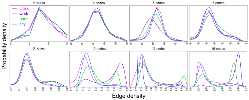
The curves correspond to the inferred priors over the density of connections only (i.e., no graphical structure) for a given cover story (indicated by the color of the curve) and a fixed number of nodes (indicated by the title of the subfigure). Notice the general trend from unimodal priors with decreasing mean for smaller graphs, with a second peak of larger edge density appearing for larger graphs.
Appearance of bimodality in priors over edge density.
For graphs with nodes, these priors consistently have a single peak around an average edge density that decreases with increasing number of nodes (echoing our results in figure 3 in the main text). However, for graphs with nodes, these priors become notably bimodal.
While it is tempting to draw conclusions about this “regime change”, it is worth remembering that human engagement for these larger graphs is still questionable. Sparse graphs are easier to remember as they admit a natural compression. This compression may equally well be applied to their complements (i.e., the nearly-complete graphs) by remembering the “non-edges”. Below nodes, the sparse peak and its dense complement overlap considerably. As the number of nodes increases, the dense peak is increasingly well-separated from its sparse complement. Thus, it is possible that these results are more a product of the participant’s desire to complete the task, instead of revealing a profound change in the way we represent graphs with more nodes than we have fingers.
Appendix D Markov Chain Monte Carlo with People
In this section, we first describe the assumptions of the MCMCP model in detail (section D.1). We then investigate the number of iterations needed for an MCMCP chain to converge sufficiently close to the prior as a function of relevant parameters (section D.2).
D.1 Assumptions
For the sake of completeness, we now describe the MCMCP model (section 4.1.2 and algorithm 1) and the corresponding assumptions required for the conclusion that the stationary distribution is equal to the prior. This discussion can be found in most introduction to probability books covering discrete Markov chains (e.g., Modica & Poggiolini (2012)).
First, let us recall the notation from section 4.1.2.
Let denote the space of all combinations of that participants might be given in a MCMCP experimental chain. Let denote the space of all that participants might consider when giving their responses. For simplicity, we consider both and to be discrete and finite (with cardinality and ), and denote the space of probability distributions over them as and .
For a given chain in our experiments, , the set of all partial graphs with nodes and of the pairwise relations obscured. The specific partial graph shown to the participant in the iteration/round is denoted as . Similarly, , the set of simple graphs with nodes. The specific simple graph resulting from the response of the participant in the iteration/round is denoted as .
Each round, the experimentalist uses the of the previous participant (i.e., their response) to generate noisy/partial to give to the next participant. Let denote this probabilistic map, with associated with probability distribution .
In this setup, the amount of transmitted at each iteration is fixed.171717If the amount of transmitted increases over time, then self-sustained learning can occur (as opposed to convergence to participants’ shared prior). See Chazelle & Wang (2016, 2019) for a mathematical analysis of this case. For example, for our experiments, the number of relations obscured is always the same in a given chain.
Let be the probabilistic map induced by participants responses, with associated probability distribution ). Participants are assumed to be identical Bayesian agents, sharing the same prior beliefs and knowledge about the experiment.
The “Bayesian” part of the assumptions refers to the fact that,
when presented with , participants are assumed to respond by sampling a hypothesis from their posterior distribution
| (6) |
The “identical agents” part of the assumptions implies two assumptions:
-
1.
Participants have the same shared prior over the , .
-
2.
Participants know the correct likelihood function used to generate the they observe from a , and they use it to compute .
Assumption 2 means that the participants are assumed to know the probabilistic map used by the experimentalist to generate from a . In our experiments, this simply means that they believe that the partial graphs are generated by randomly erasing a fraction of the relations of some underlying graph. This is clearly articulated during our experiments (see appendix A.5).
The transition matrix induced by the composed mapping is a time-homogeneous Markov chain over the discrete space of .
Such a Markov chain converges to a unique stationary distribution if (and only if) it is ergodic. This requires that:
-
1.
the chain is irreducible (i.e., any state/hypothesis can be reached from any other state/hypothesis with a non-zero probability in a finite number of iterations), and
-
2.
the chain is aperiodic.
For MCMCP experiments, we argue that both assumptions are fairly realistic. If participants have a non-zero probability of doing something completely unexpected, assumption 1 is satisfied. Assumption 2 only requires that a participant be willing to be “lazy” every once in a while.
D.2 Rate of Convergence to the Prior
How many iterations does it take for a given MCMCP chain to be sufficiently close to the prior? For a small number of nodes , it is possible to enumerate all nonisomorphic graphs . In such cases, we can answer the question of how fast the MCMCP chain converges to the prior in terms of the (asymptotic) mixing time, which we define as the time it takes for the distribution to get a factor of closer (in total variation distance) to the prior (in the limit of a large number of iterations).
For a given choice of prior over these graphs, one can explicitly construct a transition matrix representing the composed mapping . Then the mixing time is given by:
| (7) |
where is the second largest eigenvalue of .
As illustrated in figure 10, for the simplest case of an Erdős–Rényi distribution , the prior converges relatively quickly and convergence depends only on the fraction of relations obscured (independent of the number of nodes and edge density ). The exact expression for the asymptotic mixing time in this case is:
| (8) |
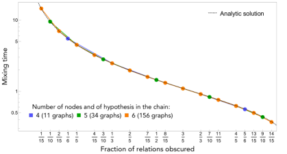
Colored markers are the values for the asymptotic mixing times (eq. 7), as a function of the fraction of relations obscured , for MCMCP chains over graphs with to nodes and with Erdős–Rényi () priors (using ) The dotted black curve is the analytic solution (eq. 8). For priors, the chains converge to the prior at a rate that depends only on the fraction of relations obscured , independent of the number of nodes and edge density .
Nevertheless, as illustrated in figure 11, for priors with even a moderate amount of structure (the priors used in that simulations are only sensitive to the edge distribution), the mixing time can vary many orders of magnitude depending on the shape of the prior and the number of relations obscured in the partial graph.
More generally, there is a delicate balance when using MCMCP experiments to recover priors. If the experimentalist obscures too little , they may never know if the experiment sufficiently reached convergence (since the shape of the true prior is unknown). On the other hand, obscuring too many could result in an experiment that is too underconstrained for participants to adequately engage and provide their true prior.
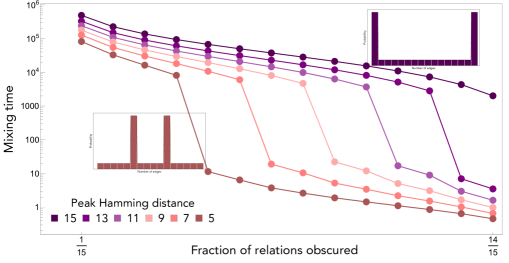
We computed the asymptotic mixing times (eq. 7) of MCMCP chains over graphs with nodes for a range of shapes for the priors (different curves) and fraction of relations obscured (vertical axis). We parameterized the priors with probabilities given by the number of edges in the graph (here, to ). In particular, we gave of the probability to graphs separated by some number of edges (the “peak Hamming distance”) and distributed the rest of the probability uniformly to the other graphs. E.g., for the prior with a peak Hamming distance of : of the probability is equally distributed between all graphs with edges, another between all graphs with edges, and the remaining between all other graphs. As expected, the higher the fraction of relations obscured, the chain mixes faster (small ). Conversely, the larger the distance (in terms of number of edges) between the peaks of the prior, the chain mixes slower.
Appendix E Advantages of Directly Modeling the Priors in MCMCP Experiments
In this section, we first demonstrate the advantages of explicitly leveraging the assumptions of the MCMCP model (section E.1). We then demonstrate the advantages of our particular choice of model for the priors (section E.2).
E.1 Exploiting the Bayesian Assumption
As discussed in section 5.1, the standard approach in MCMCP experiments is to use the observed frequency of the data towards the end of the experiments (once the chain has (hopefully) converged) as a proxy for participants priors. This wastes much of the collected data. In this section, we use some simulations to show that recovering participants priors’ by fitting the MCMCP model directly to their aggregated choices indeed uses the experimental data much more efficiently.
To compare these methods, we simulated the responses of ideal Bayesian participants (i.e., respecting all assumptions of the MCMCP model) on our MCMCP experiment over graphs with nodes and obscuring half of the relations at each iteration (i.e., ). We fit the simulated data using a distribution specifying the probability of all nonisomorphic simple graphs with nodes as the model for the prior. Our goal with these simulations is to illustrate that, when possible, it is best to recover the prior by directly fitting participants’ data to the MCMCP model (regardless of how one might choose to parameterize the prior).
As shown in figure 12,181818We use KL divergence as a measure of closeness to the prior (as opposed to, e.g., total variation distance), as it is more sensitive to relative differences in probabilities. However, the results are similar when using other measures. fitting the data to the MCMCP model (pink curves) recovers the prior more accurately than the more standard approach of using some of the observed data as a proxy for the prior (green curves). This is especially true when the chain lengths are limited (fig. 12(b)). In addition, the fitting approach does not require estimation of the mixing time, which can vary dramatically depending on the prior, number of nodes, and fraction of relations obscured (see figure 11).
In figure 13, we remove issues that are due to the burn-in period by initializing the simulated MCMCP experiments/chains with a graph sampled from the underlying prior of the simulated agents. We find that the fitting method still outperforms the standard approach, even when the simulated chains have length much longer than the mixing time. Indeed, even with the burn-in period removed, neighboring data points in a MCMCP chain are correlated.191919Asymptotically, one can approximate the effective sample size by dividing the total number of data points by the mixing time, although more precise estimates exist (for example, see Hsu et al. (2015)). This results in a decrease in the effective number of samples obtained from such an experiment.
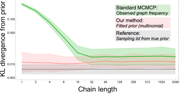
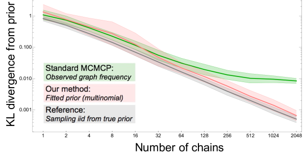
We simulated the responses of ideal participants (i.e., respecting all assumptions of the MCMCP model) on our MCMCP experiment over graphs with nodes with half of the relations obscured at each iteration, using a prior with an asymptotic mixing time of iterations. For each simulation, we fit the resulting data by maximum likelihood estimation using a distribution specifying the probability of all nonisomorphic simple graphs with nodes as the model for the prior. We then computed the KL divergence from the true prior (used to simulate the data) to: the fitted prior (in pink); the observed frequency of graphs (in green); and (as a reference) the distribution obtained by sampling i.i.d. from the true prior the same number of times (in gray). Shading denotes standard deviation about the mean for simulations for a given choice of parameters.
(a) For each position in the curve, we varied the length of the simulated chains, but kept the number of data points (i.e., the simulated agents’ answers) fixed to . While using the observed frequency is clearly doomed to fail when the length of a chain is shorter than the mixing time , fitting the data still does better even when the length is much longer than .
(b) We kept the chain length fixed to and varied the number of data points. As the number of data points increases, fitting the prior continues to improve, while using the observed graph frequency asymptotes to some finite error. This asymptote is mainly due to the contribution from graphs in the beginning of the chains.
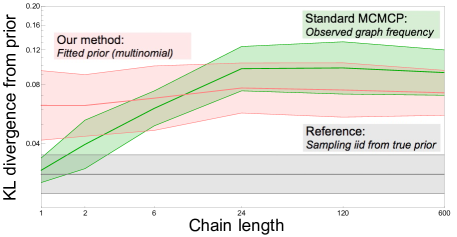
We generated synthetic data using the same specification as in figure 12, but starting with artificially pre-converged chains, by initializing the chains using a graph sampled from the true prior. For each position in the curve we varied the length of the simulated chains, but kept the number of data points fixed to . When the chain length is one, the perfect initialization renders the standard approach almost equivalent to sampling i.i.d. from the true prior. However, as the chain length increases, correlations between neighboring samples result in a decrease in the effective sample size, and the error when using the standard MCMCP sampling approach increases. When the chain length is , recovering the prior by directly fitting the MCMCP model to the data outperforms the standard approach.
E.2 Prior Parameterization
In this section, we demonstrate two practical advantages of our hierarchical parameterization for the prior (equation 1). In particular, as shown in figure 14, this parameterization results in more accurate recovery of the prior in simulated data (where we know the ground truth), and as shown in figure 15, it also improves generalization in the real data.
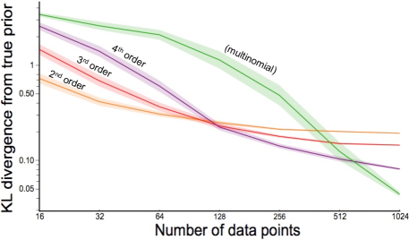
We simulated data on our MCMCP experiment over graphs with nodes (there are nonismorphic graphs in total). We then fit the MCMCP model to these simulated data using our hierarchical parameterization of the prior (eq. 1) for several choices of order . Larger corresponds to more constrained subgraph densities, thus more structured/complex priors. (For nodes, constrains all subgraph densities). Shading corresponds to standard error about the mean for runs of this simulation. When the data are limited, the model with fewer parameters recovers the prior more accurately. As the quantity of data increases, the ordering incrementally inverts until the model with highest complexity does best. However, as the number of parameters in a full multinomial model is super-exponential in the number of nodes (see table 3), and engaged human attention is expensive and difficult to obtain, the optimal order will typically be intermediate.
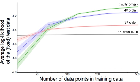
We used data points from participants doing our experiment over graphs with nodes. We randomly partitioned the data into test ( data points) and training data. We then fit the MCMCP model to the training data using our hierarchical parameterization of the prior (eq. 1) for several choices of order , and evaluated their log-likelihood in the same fixed test data. Shading corresponds to standard error about the mean for repetitions of this process. In accord with the bias-variance tradeoff, when the data are limited, using a lower-order/simpler model for the prior results in better generalization (i.e., higher log-likelihood of the unseen data). However, as the number of data points increases, higher-order/more structured priors do increasingly better. Again, in practice, the optimal order is typically intermediate.