Constraining the hadronic properties of star-forming galaxies above $1\,\rm GeV$ with 15-years Fermi-LAT data

Abstract

Context. Star-forming and starburst galaxies (SFGs and SBGs) are considered to be powerful emitters of non-thermal $\gamma$-rays and neutrinos, due to their intense phases of star-formation activity, which should confine high-energy Cosmic-Rays (CRs) inside their environments. On this regard, the Fermi-LAT collaboration has found a correlation between the $\gamma$-ray and infrared luminosities for a sample of local sources. Yet, the physics behind these non-thermal emission is still under debate.

Aims. We aim at refining the correlation between $\gamma$-rays and star formation rate (SFR) exploiting 15 years of public Fermi-LAT data, thus probing the calorimetric fraction $F_{\rm cal}$ of high-energy protons in SFGs and SBGs. Further, we aim at extrapolating this information to their diffuse $\gamma$-ray and neutrino emissions constraining their contribution to the extra-galactic gamma-ray background (EGB) and the diffuse neutrino flux.

Methods. Using the publicly-available fermitools, we analyse 15.3 years of $\gamma$-ray between $1-1000\,\rm GeV$ data for 70 sources, 56 of which were not previously detected. We relate this emission to a physically-motivated model for SBGs in order to constrain $F_{\rm cal}$ for each source and then study its correlation with the star formation rate of the sources.

Results. Firstly, we find at $4\sigma$ level an indication of $\gamma$-ray emission for other two SBGs, namely M 83 and NGC 1365. By contrast, we find that, with the new description of background, the significance for the $\gamma$-ray emission of the previously detected M 33 reduces at $4\sigma$. We also find that the physically-motivated model for $F_{\rm cal}$ correctly describes the $\gamma$-ray observations, and it is crucial to assess the systematic uncertainty on the star formation rate. Finally, undiscovered sources strongly constraints $F_{\rm cal}$ at 95% CL, providing fundamental information when we interpret the results as common properties of SFGs and SBGs. Hence, we find that these sources might contribute $(20\pm 5)\%$ to the EGB, while the corresponding diffuse neutrino flux strongly depends on the spectral index distribution along the source class.

1 Introduction

Star-forming and starburst galaxies (SFGs and SBGs) are galaxies in a phase of intense star formation, leading to high gas density and to an enhanced rate of supernovae (SN) explosions Peretti et al. (2019). This activity is expected to be directly correlated to $\gamma$-rays and neutrinos, via proton-proton (pp) collisions between high-energy Cosmic-Rays (CRs) accelerated by supernovae remnants (SNRs) and the gas (Peretti et al., 2019, 2020; Ambrosone et al., 2021a, b; Kornecki et al., 2020, 2022). The Fermi-LAT collaboration has indeed detected a sample of 14 SFGs which feature a correlation between the $\gamma$-ray luminosity from $100\,\rm MeV$ to $100\,\rm GeV$ $(L_{[0.1-100]\,\rm GeV})$ and the infrared luminosity $(L_{8-1000\,\mu\rm m})$ (Ackermann et al., 2012). These detections have also been updated by several authors, such as (Rojas-Bravo & Araya, 2016; Ajello et al., 2020; Xiang et al., 2023).

These results are typically interpreted as an evidence for the existence of common properties shared by the entire population of SFGs and SBGs (Kornecki et al., 2022). For instance, the fact that these sources present hard power-law spectra $E^{-\gamma}$, with $\gamma\sim 2.2-2.3$, might indicate that the physics of CRs is dominated by energy-independent mechanisms, such as the pp inelastic timescale or advection (Lacki & Beck, 2013). However, some works (Krumholz et al., 2020; Roth et al., 2021, 2023) have recently proposed that CR transport inside these source might be dominated by diffusion for $E_{\rm CR}\geq 100\,\rm GeV$, leading to a suppression of the $\gamma$-ray and neutrino production rates at higher energies. Physically, this means that the calorimetric fraction $F_{\rm cal}$ – i.e. the fraction of high-energy CRs which actually lose energy inside SFGs and SBGs producing $\gamma$-rays and neutrinos – might be smaller than previously predicted and also energy-dependent. In order to discriminate these two scenarios, however, new and more precise measurements (especially in the TeV energy range) are required (Ambrosone et al., 2022).

In this paper, we provide new constraints on the calorimetric fraction of SFGs and SBGs by analysing a catalogue of 70 sources introduced by Ackermann et al. (2012), using $\sim 15.3\,\rm years$ of Fermi-LAT data and the publicly-available fermitools. In particular, we search for $\gamma$-ray emission between $1\,\rm GeV$ and $1\,\rm TeV$, dividing the catalogue in two samples: the 56 sources not yet detected  and the 14 sources which have been previously detected. We find strong hints of $\gamma$-ray emission in coincidence of M 83 and NGC 1365 at level of $\sim 4\sigma$. Furthermore, for M 33 which was previously reported as a discovered source by Ajello et al. (2020), we find that its gamma-ray emission stands right below the $4\sigma$ detection level.

Then, we test a physically-motivated relation between $F_{\rm cal}$ and the rate of supernovae explosion $R_{\rm SN}$, in contrast with the simplistic power-law function previously tested (Ackermann et al., 2012; Rojas-Bravo & Araya, 2016; Ajello et al., 2020; Xiang et al., 2023), finding a good agreement with the data. We emphasise that the correct estimate of the systematic uncertainty on $\rm R_{\rm SN}$ is crucial in order to extract the correct information on this correlation. Moreover, undiscovered sources place strong constraints to $F_{\rm cal}$, thus slightly modifying the $F_{\rm cal}$–$R_{\rm SN}$ correlation. Therefore, in order to interpret these emissions as shared properties of all SFGs and SBGs is also important to take into account sources which present no evidence for $\gamma$-ray emission.

Finally, we employ such a correlation to evaluate the diffuse $\gamma$-rays and neutrinos flux from the whole source population. In order to do this, we make use of the recently-updated cosmic star-formation-rate distribution obtained through the James Webb Space Telescope reported by Kim et al. (2023). We find that SFGs and SBGs might contribute $(20\pm 5)\%$ to the extragalactic gamma-ray background (EGB) (Ackermann et al., 2015) above $50\,\rm GeV$, while their contribution to the diffuse neutrino flux measured by IceCube with 6-year cascade events (Aartsen et al., 2020) might vary from 8% to 35% crucially depending on the assumed distribution of the spectral indexes along the source class.

The paper is structured as follows. In Sec. 2, we describe the sample of galaxies analysed. In Secs. 3 and 4, we describe the statistical analysis of the Fermi-LAT data and report the corresponding results, respectively. In Sec. 5, we discuss the theoretical model we adopt to evaluate the $\gamma$-ray and neutrino fluxes from each source. In Sec. 6, we describe the $F_{\rm cal}$–$R_{\rm SN}$ correlation and discuss our findings. In Sec. 7, we extrapolate our results to the diffuse $\gamma$-ray and neutrino fluxes. Finally, in Sec. 8, we draw our conclusions. The paper has three appendices: in appendix A, we report all the new spectral energy distributions (SEDs) for the sources above the $5\sigma$ discovery threshold; in appendix B, we discuss the properties of the diffuse spectrum; in appendix C we comment on the impact of the systematic uncertainty affecting $R_{\rm SN}$ on our results.

2 Sample of galaxies

We investigate the gamma-ray emission of 70 sources which we divide into two samples:

• Sample A (see Tab. 1): it contains the galaxies introduced by Ackermann et al. (2012) (see also Rojas-Bravo & Araya (2016)) for which no $\gamma$-ray detection has been reported yet. These galaxies exhibit a galactic latitude coordinate $|\rm b|\geq 10^{\circ}$ and, therefore, the contamination from the diffuse galactic $\gamma$-ray emission is negligible. For these sources, we take the distances and the total infrared luminosity between $8-1000\,\rm\mu\rm m$ $(L_{\rm IR})$ from Rojas-Bravo & Araya (2016), consistently rescaled for the different hubble parameter $\rm H_{0}$ used.

• Sample B (see Tab. 2): it refers to the 14 sources discovered in $\gamma$-rays reported by Ajello et al. (2020), including also the Circinus Galaxy reported by Kornecki et al. (2020, 2022). For this sample, we use the distances and the infrared luminosity reported by Kornecki et al. (2020).

Some of these sources are not only classified as SFGs but also AGNs, with Seyfert activity. For this reason, we focus on $\gamma$-ray emission above $E\geq 1\,\rm GeV$, where the photons from seyfert activity are expected to be negligible (Inoue et al., 2019).

3 Data analysis

We analyse the latest Fermi-LAT data which have been collected in sky-survey mode from August 2008 and November 2023, from a Mission Elapsed Time 239557417 s to 720724699 s, with a total lifetime of $\sim$$15.3\,\rm years$. We select photons in the energy range $[1-1000]\,\rm GeV$, which strongly reduces the possibility of mis-identification of sources due to a limited PSF dimension of $\sim$$10^{\circ}$ at lower energies. We consider events belonging to P8R3_v3 version of the Pass 8 photon dataset and the corresponding P8R3_SOURCE_V3 instrument response functions. Data are analysed using the publicly-available fermitools provided by the Fermi-LAT collaboration and their analysis threads. We consider a $15^{\circ}\times 15^{\circ}$ Region of Interest (RoI) centred at the equatorial coordinates of each source, selecting only the data passing the filter for being considered of good-quality (DATA_QUAL>0)&&(LAT_CONFIG==1).

In order to reduce the contamination from the Earth’s limb, following the default suggestions in the fermitools, the events with zenith angle $>$$90^{\circ}$ are excluded. We emphasise that the Fermi-LAT collaboration has recently updated the selection for events above $1\,\rm GeV$, selecting events for zenith angle $<$$105^{\circ}$ (Abdollahi et al., 2020). However, we have verified that the results do not change either for sample A or for sample B, even with this new selection. Therefore, we prefer to leave the event selection suggested in the fermitools in order to work with a photon sample with higher purity.

These data are analysed following the binned maximum likelihood ratio method, which is officially released by the Fermi-LAT collaboration. The likelihood function is defined as (Malyshev & Mohrmann, 2023)

$$\mathcal{L}=\prod_{i}\mathcal{P}\left(E_{i},\,X_{i}\,|\,M_{i}(\Omega)\right)$$ (1)

where $\mathcal{P}(E_{i},\,X_{i}\,|\,M_{i}(\Omega))$ is the Poisson probability distribution function for observing a photon of a given energy $E_{i}$ and direction $X_{i}$, given the expected number of photons $M_{i}$ provided by the model which depends on the $\Omega$ parameters. The index $i$ runs over the bins for the events in the RoI. We determine the test statistic $\rm TS$ for each source as

$${\rm TS}=-2\,\ln\frac{\mathcal{L}_{0}}{\mathcal{L}}$$ (2)

where $\mathcal{L}_{0}$ is the maximised likelihood in the background-only hypothesis, namely in the hypothesis the source does not emit photons, and $\mathcal{L}$ is the maximised likelihood including the source under study. The conversion from the TS to the significance level can be performed using a chi-squared $\chi^{2}$ distribution with degrees of freedom equal to the number of the free parameters for the source model (Malyshev & Mohrmann, 2023). For instance, for power-law spectra, considering both normalisation and spectral index as free parameters, $\rm TS=25$ (also defined as discovery threshold for the TS) corresponds to $\sim 4.6\sigma$ significance.

In order to maximise the likelihood in Eq. (2), the data count maps are binned in angular coordinates, with $0.1^{\circ}$ bin per pixel, and in energy with 37 logarithmically spaced bins.  The background hypothesis comprises all the sources in the 4FGL catalogue gll_psc_v32.fit Abdollahi et al. (2022); Ballet et al. (2023), the standard isotropic extragalactic emission iso_P8R3_SOURCE_V3_v1 and the galactic diffuse emission gll_iem_v07. In order to account for the finite dimension of the PSF, we also consider sources outside the RoI with a further radius of $5^{\circ}$. As suggested by Malyshev & Mohrmann (2023), the fit is performed in an iterative way and at each step sources with very low $\rm TS$, such as spurious solutions with $\rm TS<0$, are eliminated from the likelihood.

In this work, for the signal hypothesis, we test power-law spectra $\phi_{\gamma}=\phi_{0}\,E^{-\gamma}$ added at the nominal position of the source. In the likelihood maximisation, we fit all the sources leaving free the source parameters (normalisation $\phi_{0}$ and spectral index $\gamma$) within $5^{\circ}$ of the RoI centre. Furthermore, we leave free the normalisation of extremely variable sources up to $15^{\circ}$ of the RoI centre  as well as the normalisation for the isotropic extragalactic and the galactic diffuse templates. The other parameters are fixed the others to their best-fit values. Finally, we also account for the energy dispersion using edisp_bins = -2 as advised in the fermitools threads. All the sources except for the Small Magellanic Cloud (SMC) and the Large Magellanic Cloud (LMC) are considered as point-like sources. For SMC and LMC, we instead utilise the official templates provided in the 4FGL catalogue. For these sources, we leave the source parameters to be free within $8^{\circ}$ and $6^{\circ}$ from the RoI centres, respectively.

4 Results of the statistical analysis

We report the obtained results in Tabs. 1 and 2 for the sample A and B, respectively. For each source of the sample A for which the TS is smaller than the discovery threshold ($\rm TS<25$), we report the luminosity distance, the infrared luminosity, and the $95\%$ CL upper limit on the flux in the range $1-1000\,\rm GeV$ assuming a spectral index $\gamma=2.3$ as typical value for known SBGs (see results for the sample B). We do not find any excess, except for M83 and NGC 1365 which shows $\rm TS\sim 15$. For these cases, we also report the best-fit values and the $68.3\%$ CL limits in brackets. Differently from Blanco et al. (2023), we do not find any hint for NGC 3079: this is probably due to the fact that they look for photons with $E\geq 50\,\rm MeV$ where the limited Fermi-LAT PSF might cause mis-identification of source. This problem has already been studied by Rojas-Bravo & Araya (2016) who pointed out that increasing the energy threshold leads to a better probe of the emission from single sources (and potentially reducing previous evidence of emission). Moreover, we find no evidence for $\gamma$-ray emission from the sources NGC 6946 and IC 342 which correlates with the most energetic CRs observed (Abbasi et al., 2023).

Source	$D_{L}$	$L_{\rm IR}$	$F^{95\%\rm CL}_{1-1000\,\rm GeV}$	$\gamma$
	$\rm[Mpc]$	$\rm[10^{10}\,L_{\odot}]$	$\rm[10^{-11}\,\rm ph\,\rm cm^{-2}\,\rm s^{-1}]$
NGC 3079	17.9	5.3	10.4	2.3
NGC 4631	8.97	2.45	5.3	2.3
M 83	4.1	1.72	$17.7\leavevmode\nobreak\ (11\pm 6)$	$2.3\leavevmode\nobreak\ (2.2\pm 0.2)$
M 51	10.6	5.15	7.28	2.3
NGC 3628	8.4	1.22	5.81	2.3
NGC 4826	5.2	0.32	6.62	2.3
NGC 6946	6.1	1.96	2.16	2.3
NGC 2903	6.9	1.02	9.72	2.3
NGC 5055	8.1	1.35	7.91	2.3
IC 342	4.1	1.72	6.80	2.3
NGC 4414	10.3	0.99	3.96	2.3
NGC 891	11.4	3.19	13.8	2.3
NGC 3893	15.4	1.47	3.21	2.3
NGC 3556	11.7	1.72	3.67	2.3
NGC 1365	23.0	$15.9$	$12.4\leavevmode\nobreak\ (8\pm 3)$	$2.3\leavevmode\nobreak\ (2.4\pm 0.2)$
NGC 660	15.5	4.5	13.6	2.3
NGC 5005	15.5	1.71	6.26	2.3
NGC 1055	16.4	2.57	13.2	2.3
NGC 7331	16.6	4.29	10.3	2.3
NGC 4030	18.9	2.57	4.38	2.3
NGC 4041	19.9	2.08	5.50	2.3
NGC 1022	23.4	3.19	3.55	2.3
NGC 5775	23.6	4.66	5.01	2.3
NGC 5713	26.6	5.15	1.55	2.3
NGC 5678	30.8	3.68	4.35	2.3
NGC 520	34.4	10.4	2.89	2.3
NGC 7479	39.0	9.1	11.2	2.3
NGC 1530	39.2	5.76	4.69	2.3
NGC 2276	39.3	7.60	5.26	2.3
NGC 3147	43.7	7.60	2.20	2.3
IC 5179	51.2	17.16	11.4	2.3
NGC 5135	57.2	17.16	8.89	2.3
NGC 6701	62.9	13.48	4.21	2.3
NGC 7771	66.9	25.7	8.18	2.3
NGC 1614	70.0	47.8	10.5	2.3
NGC 7130	72.0	25.7	1.82	2.3
NGC 7469	74.7	50.3	3.94	2.3
IRAS 18293  3413	79.8	66.2	2.14	2.3
MRK 331	83.4	33.1	1.02	2.3
NGC 828	83.5	27.0	4.33	2.3
IC 1623	90.5	57.6	3.24	2.3
ARP 193	102.6	45.4	3.16	2.3
NGC 6240	108.6	74.8	3.68	2.3
NGC 1144	129.9	30.6	3.01	2.3
MRK 1027	136.7	31.9	2.84	2.3
NGC 695	147.8	57.6	6.58	2.3
ARP 148	158.7	44.1	8.18	2.3
MRK 273	168.5	159.4	4.77	2.3
UGC 05101	177.4	109.1	4.97	2.3
ARP 55	180.1	56.4	4.90	2.3
MRK 231	188.6	367.8	5.70	2.3
IRAS 05189  2524	188.6	147.1	5.08	2.3
IRAS 17208  0014	191.7	281.9	12.3	2.3
IRAS 10566+2448	191.9	115.3	3.76	2.3
VII Zw 31	247.3	106.6	1.69	2.3
IRAS 23365+3604	294.6	171.6	11.4	2.3

Table 1: Results for the sample A. From left to right: the source name, the luminosity distance, the infrared luminosity, the upper limit on the integrated $\gamma$-ray flux, the spectral index assumed to evaluate the upper limit. For hints of $\gamma$-ray emissions, we report the best-fit values in brackets.

Source	$D_{L}$	$L_{\rm IR}$	$F_{1-1000\,\rm GeV}$	$\phi_{0}$	$\gamma$	$\rm TS\leavevmode\nobreak\ (\sigma)$
	$\rm[Mpc]$	$\rm[10^{10}\,L_{\odot}]$	$\rm[10^{-10}\,\rm ph\,\rm cm^{-2}\,\rm s^{-1}]$	$[10^{-12}\,\rm MeV^{-1}\,\rm cm^{-2}\,\rm s^{-1}]$
M 82	3.53	5.6	$9.8\pm 0.5$	$1.31\pm 0.10$	$2.34\pm 0.06$	1104 (33)
NGC 253	3.56	3.6	$8.1\pm 0.9$	$1.08\pm 0.10$	$2.33\pm 0.08$	730 (27)
ARP 220	81	$1.6\cdot 10^{2}$	$1.6\pm 0.6$	$(2.0\pm 0.7)\cdot 10^{-1}$	$2.2\pm 0.2$	50 (7.1)
NGC 1068	10.1	10.0	$4.5\pm 0.5$	$(5.8\pm 0.9)\cdot 10^{-1}$	$2.28\pm 0.15$	238 (15)
Circinus	4.21	1.7	$5.1\pm 1.3$	$(6.2\pm 1.7)\cdot 10^{-1}$	$2.23\pm 0.14$	78 (8.8)
SMC	0.06	$7.1\cdot 10^{-3}$	$(3.0\pm 0.3)\cdot 10^{1}$	$4.4\pm 0.3$	$2.44\pm 0.06$	801 (28)
M 31	0.77	$2.3\cdot 10^{-1}$	$3.1\pm 0.8$	$(6.3\pm 1.3)\cdot 10^{-1}$	$3.0\pm 0.3$	74.6 (8.6)
NGC 2146	17.2	12.6	$1.3\pm 0.5$	$(1.5\pm 0.5)\cdot 10^{-1}$	$2.16\pm 0.18$	41.5 (6.4)
ARP 299	46.8	72	$1.3\pm 0.5$	$(1.7\cdot 0.6)\cdot 10^{-1}$	$2.3\pm 0.2$	46.4 (6.8)
NGC 4945	3.72	2.8	$9.6\pm 1.3$	$1.34\pm 0.15$	$2.40\pm 0.08$	412 (20)
NGC 2403	3.18	0.15	$1.5\pm 0.5$	$(10\pm 4)\cdot 10^{-2}$	$1.92\pm 0.17$	52.8 (7.3)
NGC 3424	25.6	1.9	$10\pm 5$	$(1.3\pm 0.5)\cdot 10^{-1}$	$2.3\pm 0.3$	28 (5.3)
LMC	0.05	$5.2\cdot 10^{-2}$	$(1.38\pm 0.07)\cdot 10^{2}$	$(1.85\pm 0.08)\cdot 10^{1}$	$2.41\pm 0.04$	1493 (38)
M 33	0.91	0.14	$1.2\pm 0.6$†	$(1.8\pm 0.7)\cdot 10^{-1}$	$2.5\pm 0.3$	16 (4)

Table 2: Results for the sample B. From left to right: the source name, the luminosity distance, the infrared luminosity, the integrated $\gamma$-ray flux, the flux normalisation, the spectral index, the value of the test statistics. ^†Note that since M 33 is below the discovery threshold, we also compute the $95\%$ CL upper limit fixing $\gamma=2.3$, obtaining $F_{1-1000\,\rm GeV}=1.65\cdot 10^{-10}\,\rm ph\,\rm cm^{-2}\,\rm s^{-1}$.

For each source of the sample B, we also report the best-fit interval of the flux normalisation and spectral index at $68.3\%$ CL, and the corresponding value for the test statistics TS. Our results are in fair agreement with previous ones (Ackermann et al., 2017; Ajello et al., 2020; Abdollahi et al., 2022). For SMC, we find a slightly softer spectrum than Ajello et al. (2020) being in agreement with Abdollahi et al. (2022). We emphasise that for SMC and LMC we find convergence even though previous analyses have reported their spectra as log parabola rather than power-laws (Ajello et al., 2020). For M 31, even though it has been previously discovered as an extended source with a radius of $0.4^{\circ}$ (Ackermann et al., 2017; Ajello et al., 2020), we have used the point-like model present in the 4FGL. We obtain convergence anyway (with a $\rm TS\sim 75$), although with a very soft power-law spectrum $\sim E^{-3.0\pm 0.3}$. Finally, for M 33, there is not any match with sources present in the 4FGL catalogue. So, as for the sources in the sample A, we have added a point-like source in its position. Differently from Ajello et al. (2020), we find only an excess with $({\rm TS}\sim 16)$ which is below the discovery threshold. In appendix A, we report the SEDs for each source above the discovery threshold according to our analysis.

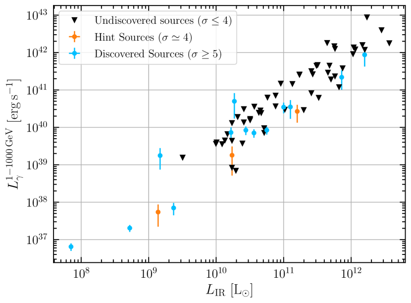
For all the sources, we compute the $\gamma$-ray luminosity $L_{\gamma}$ between $1-1000\,\rm GeV$, using

$$L^{1-1000\leavevmode\nobreak\ {\rm GeV}}_{\gamma}=4\pi\frac{D^{2}_{L}(z)}{(1+z)^{2-\gamma}}F_{1-1000\leavevmode\nobreak\ {\rm GeV}}$$ (3)

where

$$F_{1-1000\leavevmode\nobreak\ {\rm GeV}}=\int_{1\,\rm GeV}^{1000\,\rm GeV}E\,\frac{{\rm d}F}{{\rm d}E}\,{\rm d}E$$ (4)

is the integration of the differential flux measured weighted by the energy, and $z$ is the redshift of the source, directly related to the luminosity distance $D_{L}(z)$. Fig. 1 shows the $L_{\gamma}$ in the energy range $[1,\,1000]\leavevmode\nobreak\ {\rm GeV}$ versus the $L_{\rm IR}$ for the samples A and B. We report the best-fit values and the corresponding $1\sigma$ uncertainty for all the discovered sources as well as for the three sources which give us a $4\sigma$ hint of emission. On the other hand, for the undiscovered sources, we report the $95\%$ CL upper limit assuming a $E^{-2.3}$ spectrum. In the plot, we also take into account a $10\%$ uncertainty in each distance and $5\%$ in $L_{\rm IR}$ as reported by Ajello et al. (2020).

Figure 1: The $\gamma$-ray luminosity as a function of the total infrared luminosity for the entire sample. Cyan points represent discovered sources with a significance level of $\sigma\geq 5$, while orange points denote hint sources with a significance level of approximately $\sigma\simeq 4$. In both cases, the best fit scenarios along with their $1\sigma$ uncertainty are considered. For undiscovered sources ($\sigma\leq 4$), represented by black triangles, we provide $95\%$ confidence level upper limits, fixing $\gamma=2.3$.

5 Non-thermal emission from SFGs and SBGs

The results presented in the previous section have important repercussion on the CR transport mechanisms occurring inside these sources. Indeed, since photons produced by hadronic interactions usually carry $10\%$ of the parent energy of CRs, the $\gamma$-ray spectra are expected to inherit the properties of the CR distribution inside the sources. In order to assess such implications, we use a model describing the non-thermal emission of the sources. In general, since we expect the emission of SBGs to be dominated by their nuclei, we can neglect the spatial dependence of the CR diffusion. Hence, we can study the CR transport under the leaky-box model equation where the CR transport is modelled by a balance among different competing processes: the injection term of the sources such as SNRs, the escape phenomena (advection and diffusion) and the energy-loss mechanism such as hadronic collisions:

$$\frac{N_{\rm CR}(E)}{\rm\tau_{\rm esc}}+\frac{{\rm d}}{{\rm d}\rm E}\left[\frac{{\rm d}E}{{\rm d}t}\cdot N_{\rm CR}(E)\right]=Q(E)$$ (5)

where ${\rm d}E/{\rm d}t=-E/\tau_{\rm loss}$, with $\tau_{\rm loss}$ being the energy-loss timescale, $\tau_{\rm esc}$ is the escape timescale, and $Q(E)$ is the injection spectrum of SNRs which is normalised as

$$\int_{m_{p}}^{+\infty}Q(E)\,E\,{\rm d}E=\eta\,E_{\rm SN}\,R_{\rm SN}$$ (6)

Hence, the total energy injected into CRs is $\eta=10\%$ of the total $E_{\rm SN}=10^{51}\,\rm erg$ emitted by SNRs. The quantity $R_{\rm SN}$ is the SNRs rate which is expected to be tightly connected to the infrared luminosity according to the empirical relation (Kornecki et al., 2022)

$$R_{\rm SN}=\frac{1}{83}1.36\cdot 10^{-10}\left(\frac{L_{\rm IR}}{L_{\odot}}\right)\left(1+\sqrt{\frac{10^{9}\,L_{\odot}}{L_{\rm IR}}}\right)\,{\rm yr^{-1}}$$ (7)

which takes advantage of the Chabrier Initial mass function (IMF), consistent with $83\,M_{\odot}$, converted in new stars for each supernova explosion. In other words, the star formation rate (SFR) is connected to $R_{\rm SN}$ through ${\rm SFR}/(M_{\odot}\,{\rm yr^{-1}})=83\,M_{\odot}\,R_{\rm SN}/(\rm yr^{-1})$. We emphasize that Eq. 7 is not linear because the infrared luminosity itself is not a perfect tracer of the SFR.

For SBGs, pp interactions should be the dominant CR energy-loss mechanism. In this case, assuming a $Q(E)\propto E^{-\gamma}$ spectrum, Eq. (5) reads

$$N_{\rm CR}(E)=\frac{\tau_{\rm loss}}{E}\int_{E}^{+\infty}Q(E^{\prime}){\rm d}E^{\prime}=\frac{\tau_{\rm loss}\,Q(E)}{\gamma-1}$$ (8)

where $\tau_{\rm loss}=\tau_{\rm pp}$. Eq. (8) represents the general solution for sources for which any injected CR produces secondary particles through hadronic collisions (calorimetric regime). In general, sources might accomplish only partially CR calorimetry and the final CR distribution can be effectively written as (Ambrosone et al., 2022)

$$N_{\rm CR}(E)=\frac{F_{\rm cal}\,\tau_{\rm loss}\,Q(E)}{\gamma-1}$$ (9)

where $F_{\rm cal}$ is between 0 and 1. Such a quantity is a function of the dynamical timescales $\tau_{\rm loss}$ and $\tau_{\rm esc}$, which are expected to scale with the SFR (Ambrosone et al., 2021a; Kornecki et al., 2022; Krumholz et al., 2020). Hence, it can also be a function of the energy, for example in case that the escape timescales are energy dependent.

From Eq. 9, we can quantify the photon production rate following the analytical procedure of Kelner et al. (2006) (see also Kornecki et al. (2022)). For $E_{\gamma}>100\,\rm GeV$, we have

$$Q_{\gamma}(E_{\gamma})=c\,n_{\rm gas}\int_{\rm x_{\rm min}}^{1}\sigma_{pp}\left(\frac{E_{\gamma}}{x}\right)N_{\rm CR}\left(\frac{E_{\gamma}}{x}\right)\tilde{F}_{\gamma}\left(x,\frac{E_{\gamma}}{x}\right)\frac{{\rm d}x}{x}$$ (10)

where $\tilde{F}_{\gamma}\left(x,{E_{\gamma}}/{x}\right)$ is defined in (Kelner et al., 2006) (see Eqs. (58-61)) and $x_{\rm min}=10^{-3}$. For lower energies, we can assume that the pions produced by pp collisions take $K_{\pi}=17\%$ of the kinetic energy of the parent high-energy proton (delta-function approximation), having

$$\begin{split}Q_{\gamma}(E_{\gamma})&=\frac{2c\,n_{\rm gas}}{K_{\pi}}\int_{E_{\gamma}+m_{\pi}^{2}c^{4}/E_{\gamma}}^{+\infty}\frac{1}{\sqrt{E_{\pi}^{2}-m_{\pi}^{2}}}\sigma_{pp}\left(m_{p}c^{2}+\frac{E_{\pi}}{K_{\pi}}\right)\\ &\times\,N_{\rm CR}\left(m_{p}c^{2}+\frac{E_{\pi}}{K_{\pi}}\right)\,{\rm d}E_{\pi}\end{split}$$ (11)

At $E_{\gamma}=100\,\rm GeV$, Eq. (11) is scaled in order to match Eq. (10). The final $\gamma$-ray flux at Earth is given by

$$\frac{{\rm d}F_{\gamma}(E_{\gamma},z)}{{\rm d}E}=\frac{(1+z)^{2}}{4\pi D_{L}(z)^{2}}Q(E_{\gamma}(1+z))e^{-\tau(E_{\gamma},z)}$$ (12)

where $z$ is the redshift of the source, $D_{L}(z)$ is the luminosity distance, and $\tau(E,z)$ is the optical depth for photons travelling through EBL and CMB. For the computation of the opacity, we employ the model of Franceschini & Rodighiero (2017).

Analogously, from pp interactions, we expect production of high-energy neutrinos and we estimate their flux using the same procedures as for $\gamma$-rays. In particular, for $E_{\nu}>100\,\rm GeV$, we have that

$$\begin{split}Q(E_{\nu})&=\frac{1}{3}c\,n_{\rm gas}\int_{\rm x_{\rm min}}^{1}\sigma_{pp}\left(\frac{E_{\nu}}{x}\right)N_{\rm CR}\left(\frac{E_{\nu}}{x}\right)\left[\tilde{F}_{\nu^{1}_{\mu}}\left(x,\frac{E_{\gamma}}{x}\right)+\right.\\ &\left.+\tilde{F}_{\nu^{2}_{\mu}}\left(x,\frac{E_{\gamma}}{x}\right)+\tilde{F}_{\nu_{e}}\left(x,\frac{E_{\gamma}}{x}\right)\right]\,\frac{{\rm d}x}{x}\end{split}$$ (13)

where $\tilde{F}_{\nu^{1}_{\mu}}\left(x,E_{\gamma}/x\right)$, $\tilde{F}_{\nu^{2}_{\mu}}\left(x,E_{\gamma}/x\right)$ and $\tilde{F}_{\nu_{e}}\left(x,E_{\gamma}/x\right)$ takes into account all the neutrinos produced in the interactions and are defined by Kelner et al. (2006). The factor 1/3 is due to the fact that we expect an equal flavour ratio at Earth. The final neutrino flux is given by

$$\frac{{\rm d}F_{\nu}(E_{\nu},z)}{{\rm d}E}=\frac{(1+z)^{2}}{4\pi D_{L}(z)^{2}}Q_{\nu}(E_{\nu}(1+z))$$ (14)

6 On the correlation between gamma-rays and star-forming activity

In this section, we discuss our constraints on the calorimetric fraction $F_{\rm cal}$ from $\gamma$-ray observations and its correlation with $R_{\rm SN}$. Previous studies (Ackermann et al., 2012; Ajello et al., 2020; Rojas-Bravo & Araya, 2016; Xiang et al., 2023) have tested the relation $F_{\rm cal}\simeq A\left({R_{\rm SN}}/{1\,\rm yr^{-1}}\right)^{\beta}$. However, this relation cannot be valid for a wide SFR range $[10^{-3}-10^{3}]\,M_{\odot}\,\rm yr^{-1}$, since the calorimetric limit cannot be exceeded. Therefore, in the present paper we probe the following physically-motivated relation between $F_{\rm cal}$ and $R_{\rm SN}$

$$F_{\rm cal}=A\left(\frac{R_{\rm SN}}{\rm yr^{-1}}\right)^{\beta}\,\left(1+A\left(\frac{R_{\rm SN}}{\rm yr^{-1}}\right)^{\beta}\right)^{-1}$$ (15)

with $A$ and $\beta$ free parameters to be deduced from data. Such a relation comes directly from $F_{\rm cal}\simeq\left(\tau_{\rm esc}/\tau_{\rm loss}\right)\left(\tau_{\rm esc}/\tau_{\rm loss}+1\right)^{-1}$ with $\tau_{\rm esc}/\tau_{\rm loss}\simeq A\,R_{\rm SN}^{\beta}$ (Ambrosone et al., 2022; Kornecki et al., 2022; Roth et al., 2023). We notice that, for small value of $R_{\rm SN}$, Eq. (15) becomes consistent with a pure power-law relation as tested by previous study.

In order to test Eq. (15), for each source we estimate $R_{\rm SN}$ from the infrared luminosity according to Eq. (7) and we calculate the calorimetric fraction as described in Eq. (9) by matching the measured integrated spectrum with the theoretical one using the model described in the previous section. These $F_{\rm cal}$ values can be interpreted as an average calorimetric fraction between $10\leq E_{\rm CR}/{\rm GeV}\leq 10^{4}$ that is the energy range corresponding to photons emitted between $[1-1000]\,\rm GeV$. Current Fermi-LAT data are not sensitive enough to probe an energy-dependent calorimetric fraction as they are not able to probe spectra more complicated than power-laws. For the discovered sources (sample B), we evaluate the best-fit scenario and the $\pm 1\,\sigma$ values. For the undiscovered sources (sample A), we utilise the best-fit scenario for the fixed $\gamma=2.3$ and for the uncertainty, we consider the difference between $F^{95\%\rm CL}$ and $F^{\rm best}$.

In addition to the statistical uncertainties inferred by Fermi-LAT data, we also take into account the systematic uncertainties affecting $F_{\rm cal}$. On this regard, uncertainties on the source distance and rate of supernovae explosions as well as the detector systematics play a crucial role. As we mentioned above, the distance and the infrared luminosity provide an uncertainty of the order of $10\%$ and $5\%$, respectively. By contrast, the uncertainty on $R_{\rm SN}$ might also come from the IMF and the amount of mass converted in new star from each supernova explosions. The total uncertainty on $R_{\rm SN}$ is difficult to reliably assess and it may vary within $20-40\%$ (see Ackermann et al. (2012) for further details). For the following discussion, we consider a systematic uncertainty of $20\%$ on our estimates of $F_{\rm cal}$ and in the appendix C we discuss the impact of a higher uncertainty. Regarding the detector systematic uncertainty, we consider a conservative uncertainty of $10\%$. Summing all the systematic uncertainties in quadrature, we obtain an overall $30\%$ uncertainty on each value of $F_{\rm cal}$.

Figure 2: $F_{\rm cal}$ in terms of $R_{\rm SN}$ for the whole sample. Cyan points denote discovered sources, whereas black points denote undiscovered sources. Specifically, for sources exhibiting a flux compatible with zero, we present 95% CL upper limits indicated by black triangles. For all the sources, $F_{\rm cal}$ and $R_{\rm SN}$values are reported respectively with 30% and 20% systematic uncertainties. We also report the best-fit and the corresponding $1\sigma$ uncertainty band of the fit performed over the whole sample (orange) and over discovered sources (blue).

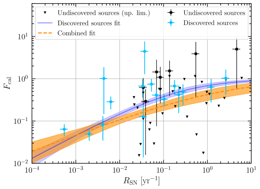
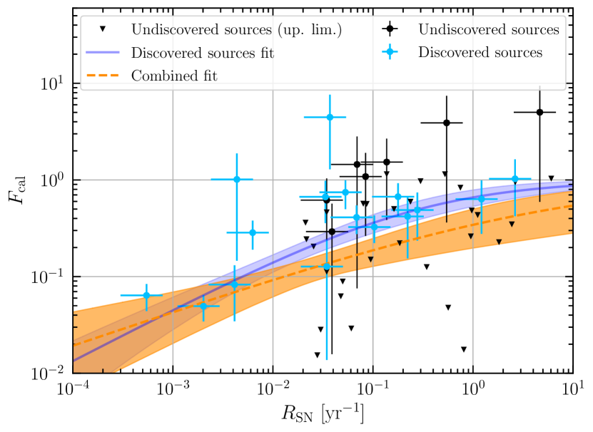
Fig. 2 shows the obtained $F_{\rm cal}$ both for undetected and detected sources as a function of $R_{\rm SN}$, as well as the $1\sigma$ bands from the fit of Eq. (15) according to two different samples of galaxies:

• Discovered sources, for which we find $A=2.2\pm 0.8$ and $\beta=0.55\pm 0.08$;

• Combined sources, namely discovered + undiscovered sources, for which we find $A=0.7_{-0.2}^{+0.3}$ and $\beta=0.39\pm 0.07$.

Interestingly, even though the undiscovered sources are characterised by higher uncertainties, they are anyway able to constrain the $F_{\rm cal}$ fit especially in the range $[0.01-1]\,\rm yr^{-1}$. In the lowest range for $R_{\rm SN}$, the fit is totally dominated by the galaxies of local group (SMC, LMC, M 31 and M 33). We can extract that $F_{\rm cal}\gtrsim 50\%$ for ${\rm SFR}\gtrsim 190_{-130}^{+1230}\,M_{\odot}\,\rm yr^{-1}$ when considering the whole sample. This might reduce the degree of calorimetry of Ultra Luminous Infrared Galaxies (ULIRGs) (sources with ${\rm SFR}\gtrsim 100\,M_{\odot}\,\rm yr^{-1}$), although, this information at the moment is mainly driven by galaxies with lower IR luminosity, since Fermi-LAT is not yet sensitive enough to directly probe the calorimetric scenario within ULIRGs, due to their large distances. We highlight that some of the sources both in sample A and B host an AGN and so their $\gamma$-ray luminosity might be contaminated by its related activity. Therefore, our results might be relatively interpreted as upper limits for $F_{\rm cal}$. Nevertheless, future measurements along with refined techniques to distinguish between star-forming and AGN related emissions will be fundamental to derive robust and final conclusions on the calorimetric nature of SFGs and SBGs (Kornecki et al., 2022).

7 Extrapolation to the diffuse emissions

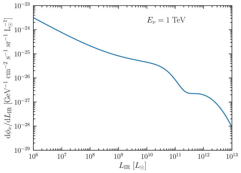
We can use the calorimetric fraction of local SFGs and SBGs evaluated in the previous section to constrain the diffuse non-thermal emission of the entire source population. The diffuse emission, per solid angle, is given by

$$\begin{split}\phi^{\rm diff}_{\gamma,\nu}=&\frac{c}{4\pi H_{0}}\int_{0}^{z_{\rm max}}\frac{{\rm d}z}{E^{2}(z)}\int_{10^{6}L_{\odot}}^{\infty}\frac{{\rm d}L_{\rm IR}}{\ln(10)\,L_{\rm IR}}\mathcal{S}_{\rm SFR}(L_{\rm IR},z)\\ &\times Q_{\gamma,\nu}\left(E(1+z),L,F_{\rm cal}(L_{\rm IR})\right)\,e^{-\tau_{\gamma,\nu}(E,z,L_{\rm IR})}\end{split}$$ (16)

where z is the redshift, $E(z)=\sqrt{\Omega_{M}(1+z)^{3}+\Omega_{\Lambda}}$, $\mathcal{S}_{\rm SFR}(L_{\rm IR},z)$ is the density of the sources as a function of the infrared luminosity, $Q_{\gamma,\nu}$ are the $\gamma$ and neutrino production rate for each source, and $\tau_{\nu}=0$ and $\tau_{\gamma}(E,z,L_{\rm IR})$ accounts for the CMB+EBL absorption of photons as well as for internal absorption phenomena (Peretti et al., 2020; Ambrosone et al., 2021b, a). We highlight that in Eq. 16 we use $L_{\rm IR}=10^{6}L_{\odot}$ as a lower limit for the infrared luminosity corresponding at ${\rm SFR}\sim 4\cdot 10^{-3}\,M_{\odot}\,\rm yr^{-1}$. Increasing such a value to $10^{10}\,L_{\odot}(\sim 1\,M_{\odot}\,\rm yr^{-1})$ results in a reduction of the flux by $\sim$$5\%$ only, since the bulk of the emission comes from sources with higher star formation rates. For the density of the sources, we use the approach described by Kim et al. (2023), who have recently updated the distribution of the cosmic SFR using also JWST data. The distribution is given in terms of a Schechter function

$$\mathcal{S}_{\rm SFR}(L_{\rm IR},z)=\Phi^{*}(z)\left(\frac{L_{\rm IR}}{L^{*}(z)}\right)^{1-\alpha}e^{-\frac{1}{2\sigma^{2}}\log_{10}^{2}\left(1+\frac{L_{\rm IR}}{L^{*}(z)}\right)}$$ (17)

which behaves as a power-law for $L_{\rm IR}\ll L^{*}(z)$ and as a Gaussian in $\log_{10}(L_{\rm IR})$ for $L_{\rm IR}\gg L^{*}(z)$. The redshift parameter evolutions are not simply set by power-laws, but rather follow skew Gaussian distributions Gruppioni et al. (2011)

$$\log_{10}(L^{*}(z)) = \log_{10}(L^{*}(0))+\frac{A_{L}}{2\pi\omega}e^{-z^{2}/(2\omega^{2})}\,{\rm erf}\left(\frac{k\,z}{\omega}\right)$$ (18)

$$\log_{10}(\Phi^{*}(z)) = \log_{10}(\Phi^{*}(0))+\frac{A_{\Phi}}{2\pi\omega}e^{-z^{2}/(2\omega^{2})}\,{\rm erf}\left(\frac{k\,z}{\omega}\right)$$ (19)

where $\text{erf}(x)$ is the error function, $k$ is called the shape parameter, $\omega$ the scale factor, $A_{L}$ and $A_{\Phi}$ are the normalisation for the evolution of $L^{*}(z)$ and $\Phi^{*}(z)$, respectively. Eqs. (18) and (19) provide physical representations of the evolution, allowing for different peaking redshifts as well as asymmetric increasing/decreasing rates for several populations Gruppioni et al. (2011). In fact, one of the main advantages of such a parameterisation is that it can be divided for distinct source classes. Here, we consider SFGs and SBGs, taking the values reported in Tab. 3. They provide excellent agreement with the ones reported by Kim et al. (2023) (see their Fig. 10). Some parameters are also in agreement with the ones reported by Gruppioni et al. (2011).

Source Class	$A_{L}$	$A_{\Phi}$	$k$	$\omega$	$\Phi^{*}(0)\,[\rm Mpc^{-3}\,\rm dex^{-1}]$	$L^{*}(0)\,[L_{\odot}]$	$\alpha$	$\sigma$
SFGs	1.01	3.79	5.11	2.40	$1.2\cdot 10^{-3}$	$3.2\cdot 10^{10}$	1,35	0.300
SBGs	11.95	8.50	3.10	3.50	$3\cdot 10^{-5}$	$1.5\cdot 10^{10}$	0.05	0.465

Table 3: Parameters defining the Schechter function in Eqs. (17), (18) and (19). The first four parameters (from left to right) are the ones reported by Kim et al. (2023), while the remaining parameters are obtained to match the SFG and SBG distributions reported in their Fig. 10.

Finally, for $F_{\rm cal}(L_{\rm IR})$ we use Eq. (15) with parameters inferred by the data of both the discovered sources and the total sample (discovered + undiscovered) sources.

Figure 3: Left: Diffuse $1\sigma$ $\gamma$-ray (dark red) and neutrino (cyan) bands predicted with the fit over the whole sample. On the left, the spectral index is fixed at $2.3$ for each source. Right: the same but considering a spectral index blending. In both panels, the fluxes are compared with the Isotropic Gamma-Ray Background (IGRB) measured by Fermi-LAT Ackermann et al. (2015), the 6 year Cascade neutrino flux Aartsen et al. (2020) and 7.5 year HESE data Abbasi et al. (2021) measured by the IceCube neutrino Observatory.

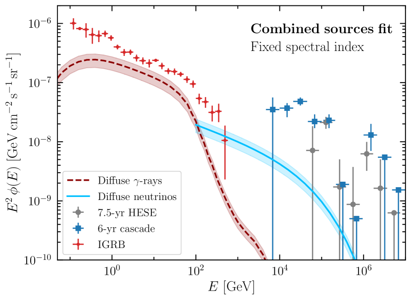
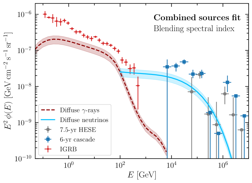
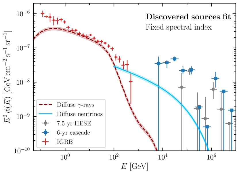
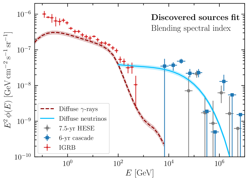
Fig. 3 shows the final $\gamma$-ray (in dark red colour) and neutrino (in cyan colour) fluxes for the combined fit including discovered and undiscovered sources, assuming a high-energy cut-off of $10\,\rm PeV$ for protons consistent with our previous results (Ambrosone et al., 2021b, 2022). On the left panel, we have fixed spectral index to $\gamma=2.3$, while on the right we have used a spectral index distribution (blending scenario) provided by a superposition of Gaussian distributions with mean values equal to the best-fit spectral index for discovered sources and with standard deviation equal to their corresponding uncertainty. The theoretical predictions are compared with the Isotropic Gamma-Ray Background (IGRB) measured by Fermi-LAT (Ackermann et al., 2015), the 6-year cascade neutrino flux (Aartsen et al., 2020) and 7.5-year HESE data (Abbasi et al., 2021) measured by the IceCube neutrino Observatory. The fluxes are dominated by distant sources with a contribution peaking at $z=1.2$. Furthermore, the bulk of the emissions come from ULIRGs saturating almost 60% of the emissions (see the appendix B for details). We find that the total contribution to the extra-galactic gamma-ray background (EBG) (Ackermann et al., 2015) between 50 GeV and 2 TeV is $\simeq(19_{-4}^{+6})\%$, almost independent on the spectral index distribution considered. The neutrino spectrum, on the contrary, is strongly dependent on the spectral index distribution. Indeed, fixing a spectral index $\gamma=2.3$ provides a soft diffuse spectrum which can explain only $(7\pm 2)\%$ of the 6-year cascade flux between 10 TeV and 1 PeV. By contrast, the spectral index blending hardens the spectrum and allows for the neutrino spectrum to explain $(36\pm 9)\%$ of the 6-year cascade IceCube flux.

Figure 4: Left: Diffuse $1\sigma$ $\gamma$-ray (dark red) and neutrino (cyan) bands predicted with the fit over discovered sources. On the left, the spectral index is fixed at $2.3$ for each source. Right: the same but considering a spectral index blending. In both panels, the fluxes are compared with the Isotropic Gamma-Ray Background (IGRB) measured by Fermi-LAT Ackermann et al. (2015), the 6 year Cascade neutrino flux Aartsen et al. (2020) and 7.5 year HESE data Abbasi et al. (2021) measured by the IceCube neutrino Observatory.

In order to assess the impact of the undiscovered sources in the $F_{\rm cal}$, in Fig. 4 we show the diffuse $\gamma$-ray and neutrino spectra obtained with the fit of the discovered sources only. In this case, we obtain that SFGs and SBGs may contribute more to the EGB and the diffuse neutrino flux, almost saturating the IGRB between $\sim 1-100\,\rm GeV$, similarly to the results of Tamborra et al. (2014); Roth et al. (2021). Therefore, undiscovered sources are not only important to correctly estimate the significance of the correlation between $F_{\rm cal}$ and $R_{\rm SN}$, but they are also necessary to correctly extrapolate information to the whole source population (Ackermann et al., 2012). This is crucial because, typically, analyses which attempts to constrain the properties of SFGs and SBGs tune their models on the sources discovered in the $\gamma$-ray range, but there are a lot of sources with the similar astrophysical properties which have not been detected and they should be taken into account if the entire source population share the same properties.

We point out that even though $F_{\rm cal}$ calculated with Fermi-LAT data corresponds to average values of $E_{\rm CR}$ between $10-10^{4}\,\rm GeV$, we extrapolate this calorimetric fraction also to higher energies in order to estimate the neutrino contribution. This, from one hand, it may be pessimistic since in case of energy-independent escape timescales, $F_{\rm cal}$ is logarithmically energy-increasing due to the energy behaviour of $\sigma_{pp}$. From the other hand, it may be optimistic since escape timescales might be energy dependent strongly suppressing the calorimetric fraction. On the whole, we find our approximation to be a reasonable trade-off. We also emphasise that Eq. (15) is considered to be valid at each redshift even though only local sources has been used to constrain it. Only future measurements will allow us to confirm if this hypothesis is correct, because at the moment Fermi-LAT is not sensitive enough to probe the calorimetric scenario for more distant sources.

8 Conclusions

In this paper, we have analysed 70 local sources, classified as star-forming and starburst galaxies, using 15 years of Fermi-LAT data. In order to reduce contamination from possible AGN activity as well as to reduce the possibility of mis-identification of sources from limited PSF, we have searched for photons with $E_{\nu}>1\,\rm GeV$. We have found evidence at $\sim$$4\sigma$ for two nearby sources, M 83 and NGC 1365. On the contrary, M 33 – a previously detected source at $\sim$$5\sigma$ – has fallen back into evidence at $4\sigma$ due to an improved treatment of the background model. We imposed strict upper limit at $95\%$ CL fixing a spectral index $\gamma=2.3$ for the other sources. Exploiting these findings, we have then revisited the correlation between the $\gamma$-ray luminosity and the star formation rate for local star-forming and starburst galaxies. For the first time, we have studied this correlation under a physically-motivated relation between the calorimetric fraction and the rate of supernova explosions. We have found that there is a good agreement between the measurements and the theoretical model and that undiscovered sources play an important role in constraining the calorimetric fraction. This is crucial in order to capture the shared properties of these sources.

Then, we have extrapolated this information to constrain the diffuse $\gamma$-ray and neutrino spectra of SFGs and SBGs, finding that they contribute about $20\%$ to the EGB above $50\,\rm GeV$. The corresponding neutrino flux is strongly dependent on the spectral index distribution along the source class. Indeed, if it is fixed at $\gamma=2.3$ for the entire source spectrum, the contribution is negligible to the diffuse neutrino flux measured by ICeCube.

By contrast, if there is a continuous distribution of this parameter within the source class, the contribution to the diffuse neutrino flux could increase by up to 40% because of sources with hard spectra. Therefore, future measurements, which aim to expand the sample of galaxies above the discovery threshold, will be essential to test how this parameter varies across the SFGs and SBGs population and to quantify its impact on the diffuse neutrino flux.

Finally, with current data we have obtained that high SFR sources have $F_{\rm cal}\gtrsim 50\%$. In fact, they mainly drive the diffuse $\gamma$-ray and neutrino fluxes. Hence, future analyses and data aiming at directly probing the degree of calorimetry of these sources are fundamental to further constrain the diffuse emission of SFGs and SBGs.

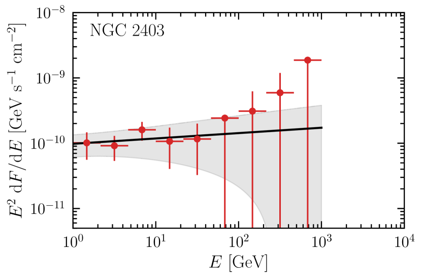
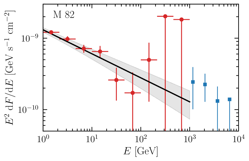
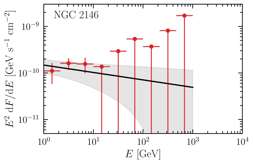
Appendix A Spectral energy distributions

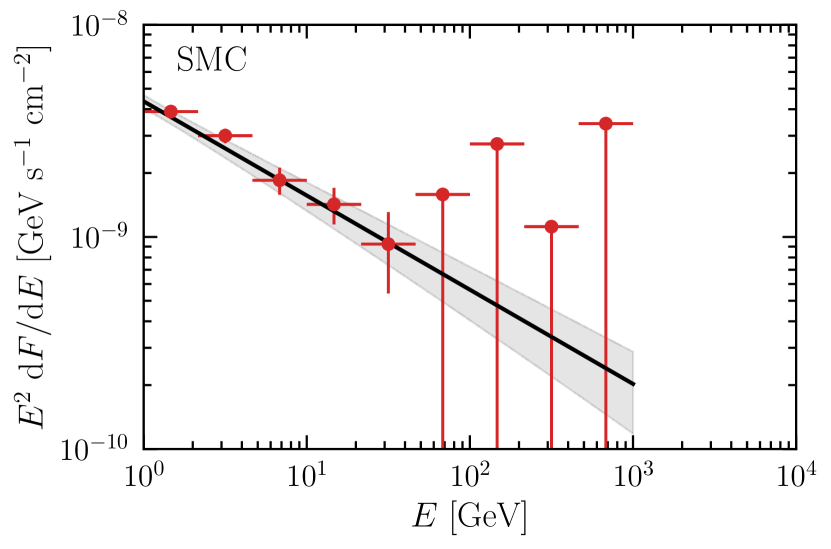
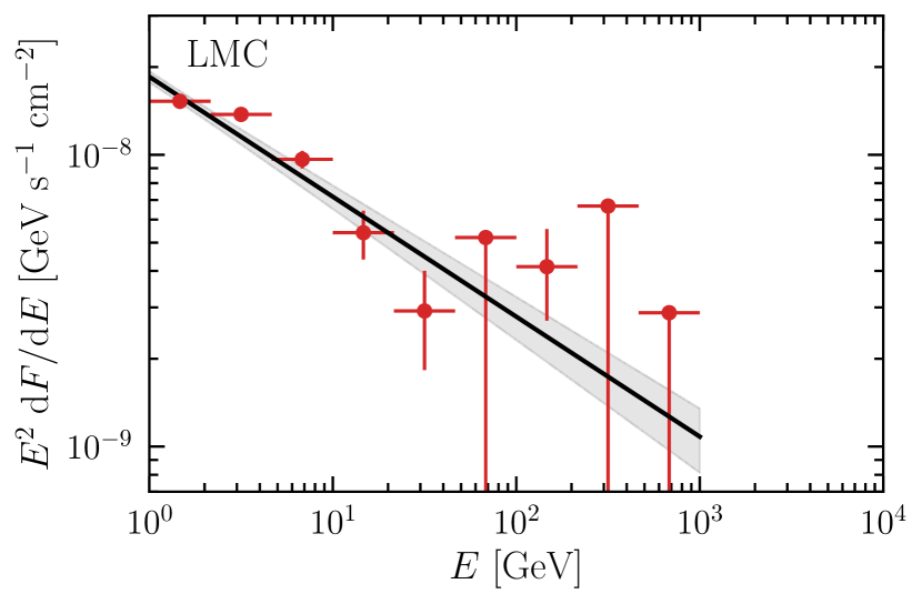
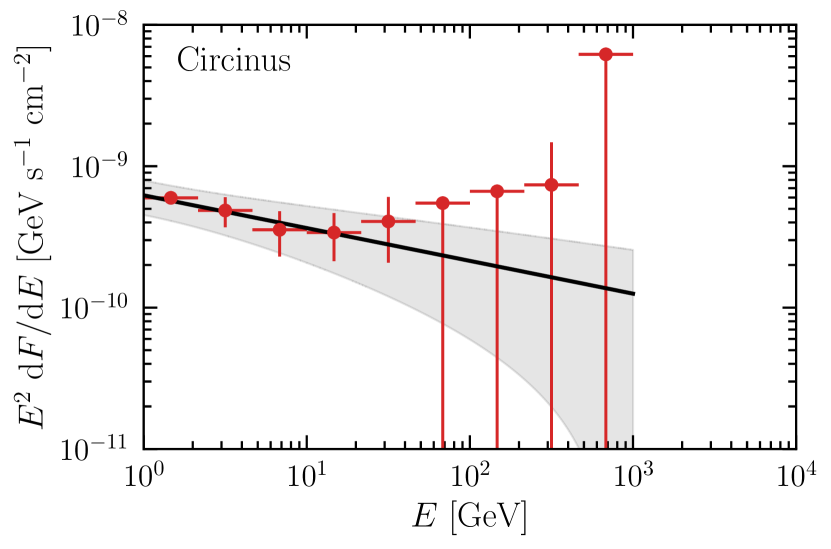
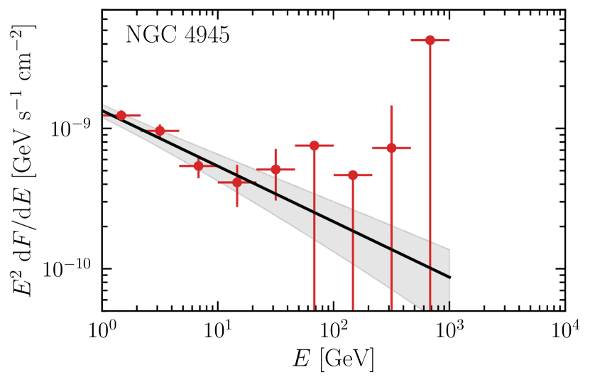
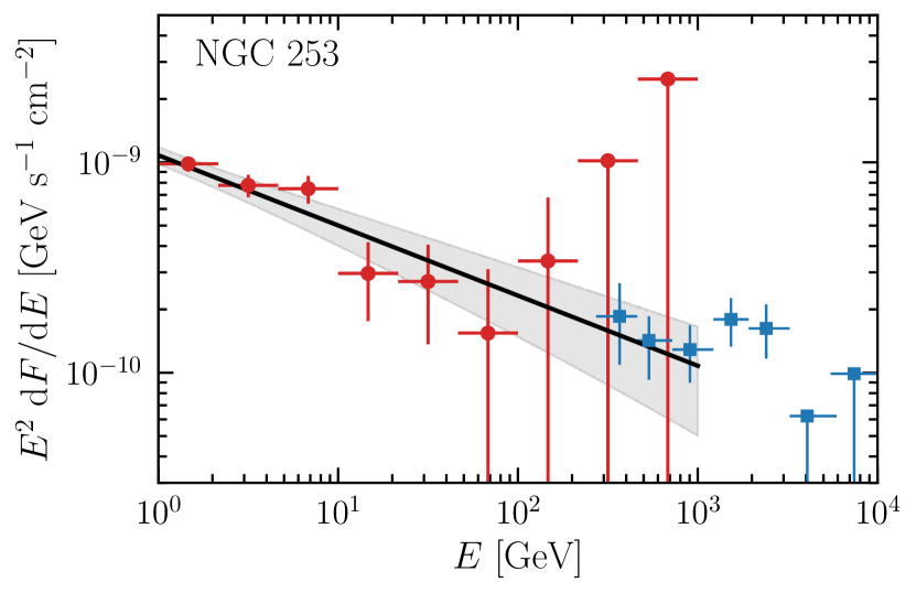
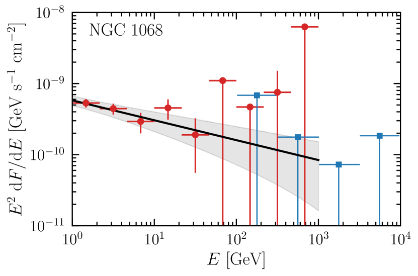
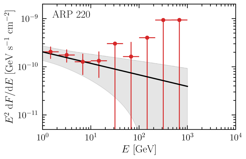
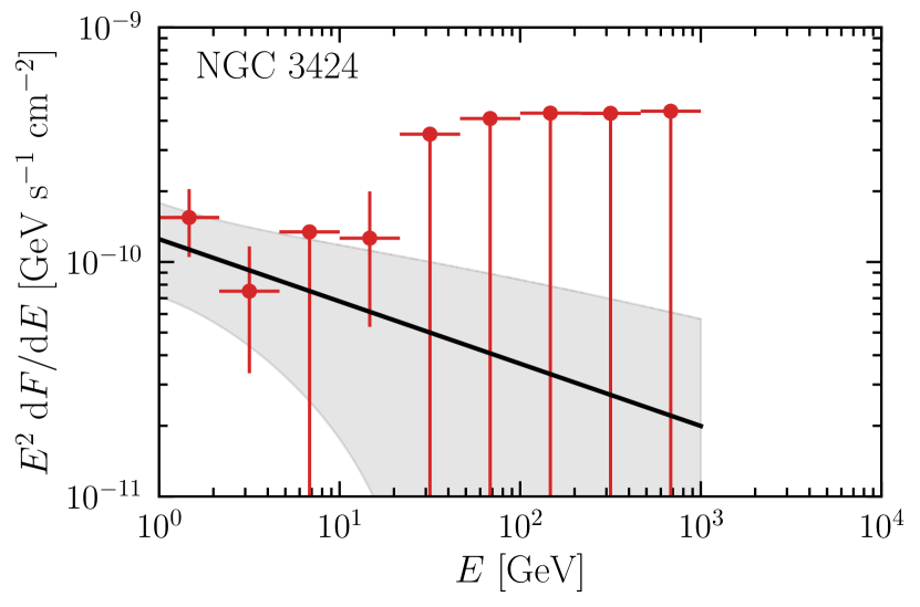
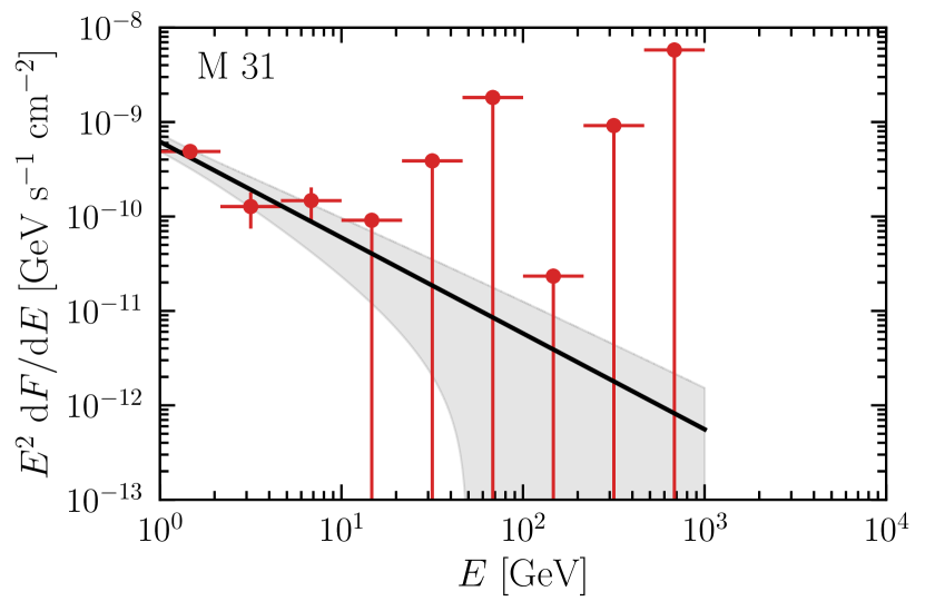
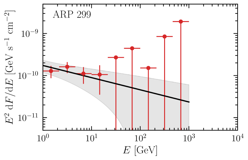
Here we report the spectral energy distributions (SEDs) for the sources above the discovery threshold. We divide the analysed energy range $[1-1000]\,\rm GeV$ in 9 independent bins (3 per decade) and perform a likelihood analysis in each bin fixing the spectral index to $\gamma=2.0$. If $\rm TS<4$, then we report the upper limit at $95\%$ CL. Our results are shown in Figs. 5 and 6, where we divide the sources in the northern hemisphere (equatorial declination $(\delta>0^{\circ}$) and in the southern hemisphere $(\delta<0^{\circ})$. The red points correspond to the best-fit Fermi-LAT measurements with the $1\sigma$ uncertainty, while the black line and the grey band respectively represent the best-fit and the $1\sigma$ band for the fit over the entire energy range. For M 82, NGC 253 and NGC 1068, we also report the measurements (in blue color) taken by VERITAS (VERITAS Collaboration et al. 2009), H.E.S.S. (Abdalla et al. 2018) and MAGIC (Acciari et al. 2019), respectively. Finally, for each source (from Tab. 4 to Tab. 16), we report the obtained TS in each energy bin and if $\rm TS>4$, we report the best-fit value of the SED and its $1\sigma$ uncertainty, otherwise we report its 95% CL upper limit.

Figure 5: Collection of the SEDs for sources situated in the southern hemisphere $(\delta<0^{\circ})$. The red points corresponds to the SED points for each energy bin, while the black line and the grey bands respectively correspond to the best fit and $1\sigma$ band for the fit over the entire energy range. For NGC 253 and NGC 1068, we also report with blue data points the H.E.S.S. measurements (Abdalla et al. 2018) and MAGIC upper limits (Acciari et al. 2019), respectively.

Figure 6: Collection of the SEDs for sources situated in the northern hemisphere $(\delta>0^{\circ})$. The red points corresponds to the SED points for each energy bin, while the black line and the grey bands respectively correspond to the best fit and $1\sigma$ band for the fit over the entire energy range. For M82, we also report with blue data points the VERITAS measurements (VERITAS Collaboration et al. 2009).

Energy range	TS	$E^{2}\leavevmode\nobreak\ {\rm d}F/{\rm d}E$	$1\sigma$ error	95% CL upper limit
$[\log_{10}(E/{\rm GeV})]$		$[\rm GeV\,\rm cm^{-2}\,\rm s^{-1}]$	$[\rm GeV\,\rm cm^{-2}\,\rm s^{-1}]$	$[\rm GeV\,\rm cm^{-2}\,\rm s^{-1}]$
0.00 - 0.33	431	$1.21\cdot 10^{-9}$	$7\cdot 10^{-11}$	–
0.33 - 0.66	362	$9.7\cdot 10^{-10}$	$9\cdot 10^{-11}$	–
0.66 - 1.00	182	$7.2\cdot 10^{-10}$	$9\cdot 10^{-11}$	–
1.00 - 1.33	106	$6.5\cdot 10^{-10}$	$1.3\cdot 10^{-10}$	–
1.33 - 1.66	20	$2.6\cdot 10^{-10}$	$1.6\cdot 10^{-10}$	–
1.66 - 2.00	5	$1.7\cdot 10^{-10}$	$1.6\cdot 10^{-10}$	–
2.00 - 2.33	11	$5\cdot 10^{-10}$	$3\cdot 10^{-10}$	–
2.33 - 2.66	3	–	–	$2.0\cdot 10^{-9}$
2.66 - 3.00	0	–	–	$1.8\cdot 10^{-9}$

Table 4: M 82: the energy range corresponding to each bin, the TS obtained for the source, the best-fit value of the SED and its $1\sigma$ error and finally the the $95\%$ CL upper limit. If $\rm TS>4$, we report the SED best-fit value and its $1\sigma$ error; otherwise we report the $95\%$ CL upper limit.

Energy range	TS	$E^{2}\leavevmode\nobreak\ {\rm d}F/{\rm d}E$	$1\sigma$ error	95% CL upper limit
$[\log_{10}(E/{\rm GeV})]$		$[\rm GeV\,\rm cm^{-2}\,\rm s^{-1}]$	$[\rm GeV\,\rm cm^{-2}\,\rm s^{-1}]$	$[\rm GeV\,\rm cm^{-2}\,\rm s^{-1}]$
0.00 - 0.33	311	$9.8\cdot 10^{-10}$	$8\cdot 10^{-11}$	–
0.33 - 0.66	212	$7.7\cdot 10^{-10}$	$9\cdot 10^{-11}$	–
0.66 - 1.00	166	$7.5\cdot 10^{-10}$	$1.1\cdot 10^{-10}$	–
1.00 - 1.33	24	$3.0\cdot 10^{-10}$	$1.2\cdot 10^{-10}$	–
1.33 - 1.66	10	$2.7\cdot 10^{-10}$	$1.3\cdot 10^{-10}$	–
1.66 - 2.00	5	$1.5\cdot 10^{-10}$	$1.5\cdot 10^{-10}$	–
2.00 - 2.33	7	$3.4\cdot 10^{-10}$	$3.4\cdot 10^{-10}$	–
2.33 - 2.66	0	–	–	$1.0\cdot 10^{-9}$
2.66 - 3.00	0	–	–	$2.5\cdot 10^{-9}$

Table 5: NGC 253: the energy range corresponding to each bin, the TS obtained for the source, the best-fit value of the SED and its $1\sigma$ error and finally the the $95\%$ CL upper limit. If $\rm TS>4$, we report the SED best-fit value and its $1\sigma$ error; otherwise we report the $95\%$ CL upper limit.

Energy range	TS	$E^{2}\leavevmode\nobreak\ {\rm d}F/{\rm d}E$	$1\sigma$ error	95% CL upper limit
$[\log_{10}(E/{\rm GeV})]$		$[\rm GeV\,\rm cm^{-2}\,\rm s^{-1}]$	$[\rm GeV\,\rm cm^{-2}\,\rm s^{-1}]$	$[\rm GeV\,\rm cm^{-2}\,\rm s^{-1}]$
0.00 - 0.33	11	$2.0\cdot 10^{-10}$	$6\cdot 10^{-11}$	–
0.33 - 0.66	14	$1.8\cdot 10^{-10}$	$5\cdot 10^{-11}$	–
0.66 - 1.00	10	$1.3\cdot 10^{-10}$	$6\cdot 10^{-11}$	–
1.00 - 1.33	11	$1.3\cdot 10^{-10}$	$7\cdot 10^{-11}$	–
1.33 - 1.66	3	–	–	$3.0\cdot 10^{-10}$
1.66 - 2.00	5	$1.6\cdot 10^{-10}$	$1.6\cdot 10^{-10}$	–
2.00 - 2.33	0	–	–	$4.0\cdot 10^{-10}$
2.33 - 2.66	0	–	–	$9.3\cdot 10^{-10}$
2.66 - 3.00	0	–	–	$9.3\cdot 10^{-10}$

Table 6: ARP 220: the energy range corresponding to each bin, the TS obtained for the source, the best-fit value of the SED and its $1\sigma$ error and finally the the $95\%$ CL upper limit. If $\rm TS>4$, we report the SED best-fit value and its $1\sigma$ error; otherwise we report the $95\%$ CL upper limit.

Energy range	TS	$E^{2}\leavevmode\nobreak\ {\rm d}F/{\rm d}E$	$1\sigma$ error	95% CL upper limit
$[\log_{10}(E/{\rm GeV})]$		$[\rm GeV\,\rm cm^{-2}\,\rm s^{-1}]$	$[\rm GeV\,\rm cm^{-2}\,\rm s^{-1}]$	$[\rm GeV\,\rm cm^{-2}\,\rm s^{-1}]$
0.00 - 0.33	75	$5.3\cdot 10^{-10}$	$7\cdot 10^{-11}$	–
0.33 - 0.66	79	$4.4\cdot 10^{-10}$	$8\cdot 10^{-11}$	–
0.66 - 1.00	24	$2.9\cdot 10^{-10}$	$9\cdot 10^{-1}$	–
1.00 - 1.33	44	$4.5\cdot 10^{-10}$	$1.4\cdot 10^{-10}$	–
1.33 - 1.66	9	$1.9\cdot 10^{-10}$	$1.3\cdot 10^{-10}$	–
1.66 - 2.00	0	–	–	$1.1\cdot 10^{-9}$
2.00 - 2.33	0	–	–	$4.7\cdot 10^{-8}$
2.33 - 2.66	9	$7.5\cdot 10^{-10}$	$7.5\cdot 10^{-10}$	–
2.66 - 3.00	3	–	–	$6.3\cdot 10^{-9}$

Table 7: NGC 1068: the energy range corresponding to each bin, the TS obtained for the source, the best-fit value of the SED and its $1\sigma$ error and finally the the $95\%$ CL upper limit. If $\rm TS>4$, we report the SED best-fit value and its $1\sigma$ error; otherwise we report the $95\%$ CL upper limit.

Energy range	TS	$E^{2}\leavevmode\nobreak\ {\rm d}F/{\rm d}E$	$1\sigma$ error	95% CL upper limit
$[\log_{10}(E/{\rm GeV})]$		$[\rm GeV\,\rm cm^{-2}\,\rm s^{-1}]$	$[\rm GeV\,\rm cm^{-2}\,\rm s^{-1}]$	$[\rm GeV\,\rm cm^{-2}\,\rm s^{-1}]$
0.00 - 0.33	16	$6.0\cdot 10^{-10}$	$6\cdot 10^{-11}$	–
0.33 - 0.66	21	$4.9\cdot 10^{-10}$	$1.2\cdot 10^{-10}$	–
0.66 - 1.00	15	$3.6\cdot 10^{-10}$	$1.3\cdot 10^{-10}$	–
1.00 - 1.33	9	$3.4\cdot 10^{-10}$	$1.3\cdot 10^{-10}$	–
1.33 - 1.66	10	$4.1\cdot 10^{-10}$	$2.0\cdot 10^{-10}$	–
1.66 - 2.00	1	–	–	$5.5\cdot 10^{-10}$
2.00 - 2.33	0	–	–	$6.6\cdot 10^{-10}$
2.33 - 2.66	5	$7.4\cdot 10^{-10}$	$7.4\cdot 10^{-10}$	–
2.66 - 3.00	3.6	–	–	$6.2\cdot 10^{-9}$

Table 8: Circinus: the energy range corresponding to each bin, the TS obtained for the source, the best-fit value of the SED and its $1\sigma$ error and finally the the $95\%$ CL upper limit. If $\rm TS>4$, we report the SED best-fit value and its $1\sigma$ error; otherwise we report the $95\%$ CL upper limit.

Energy range	TS	$E^{2}\leavevmode\nobreak\ {\rm d}F/{\rm d}E$	$1\sigma$ error	95% CL upper limit
$[\log_{10}(E/{\rm GeV})]$		$[\rm GeV\,\rm cm^{-2}\,\rm s^{-1}]$	$[\rm GeV\,\rm cm^{-2}\,\rm s^{-1}]$	$[\rm GeV\,\rm cm^{-2}\,\rm s^{-1}]$
0.00 - 0.33	481	$3.90\cdot 10^{-9}$	$1.1\cdot 10^{-10}$	–
0.33 - 0.66	241	$3.00\cdot 10^{-9}$	$2.4\cdot 10^{-10}$	–
0.66 - 1.00	73	$1.85\cdot 10^{-9}$	$2.7\cdot 10^{-10}$	–
1.00 - 1.33	27	$1.42\cdot 10^{-9}$	$2.8\cdot 10^{-10}$	–
1.33 - 1.66	7	$9\cdot 10^{-10}$	$3\cdot 10^{-10}$	–
1.66 - 2.00	2	–	–	$1.6\cdot 10^{-9}$
2.00 - 2.33	0	–	–	$2.7\cdot 10^{-9}$
2.33 - 2.66	0	–	–	$1.1\cdot 10^{-9}$
2.66 - 3.00	0	–	–	$3.4\cdot 10^{-9}$

Table 9: SMC: the energy range corresponding to each bin, the TS obtained for the source, the best-fit value of the SED and its $1\sigma$ error and finally the the $95\%$ CL upper limit. If $\rm TS>4$, we report the SED best-fit value and its $1\sigma$ error; otherwise we report the $95\%$ CL upper limit.

Energy range	TS	$E^{2}\leavevmode\nobreak\ {\rm d}F/{\rm d}E$	$1\sigma$ error	95% CL upper limit
$[\log_{10}(E/{\rm GeV})]$		$[\rm GeV\,\rm cm^{-2}\,\rm s^{-1}]$	$[\rm GeV\,\rm cm^{-2}\,\rm s^{-1}]$	$[\rm GeV\,\rm cm^{-2}\,\rm s^{-1}]$
0.00 - 0.33	58	$4.9\cdot 10^{-10}$	$7\cdot 10^{-11}$	–
0.33 - 0.66	7	$1.3\cdot 10^{-10}$	$5\cdot 10^{-11}$	–
0.66 - 1.00	11	$1.5\cdot 10^{-10}$	$6\cdot 10^{-11}$	–
1.00 - 1.33	3	–	–	$9.1\cdot 10^{-11}$
1.33 - 1.66	0	–	–	$3.9\cdot 10^{-10}$
1.66 - 2.00	0	–	–	$1.8\cdot 10^{-9}$
2.00 - 2.33	0	–	–	$2.3\cdot 10^{-11}$
2.33 - 2.66	0	–	–	$9.2\cdot 10^{-10}$
2.66 - 3.00	3	–	–	$5.8\cdot 10^{-9}$

Table 10: M 31: the energy range corresponding to each bin, the TS obtained for the source, the best-fit value of the SED and its $1\sigma$ error and finally the the $95\%$ CL upper limit. If $\rm TS>4$, we report the SED best-fit value and its $1\sigma$ error; otherwise we report the $95\%$ CL upper limit.

Energy range	TS	$E^{2}\leavevmode\nobreak\ {\rm d}F/{\rm d}E$	$1\sigma$ error	95% CL upper limit
$[\log_{10}(E/{\rm GeV})]$		$[\rm GeV\,\rm cm^{-2}\,\rm s^{-1}]$	$[\rm GeV\,\rm cm^{-2}\,\rm s^{-1}]$	$[\rm GeV\,\rm cm^{-2}\,\rm s^{-1}]$
0.00 - 0.33	5	$1.1\cdot 10^{-10}$	$5\cdot 10^{-11}$	–
0.33 - 0.66	18	$1.6\cdot 10^{-10}$	$5\cdot 10^{-11}$	–
0.66 - 1.00	17	$1.6\cdot 10^{-10}$	$6\cdot 10^{-11}$	–
1.00 - 1.33	0	–	–	$1.4\cdot 10^{-10}$
1.33 - 1.66	3	–	–	$2.9\cdot 10^{-10}$
1.66 - 2.00	3.8	–	–	$5.4\cdot 10^{-10}$
2.00 - 2.33	0	–	–	$3.7\cdot 10^{-10}$
2.33 - 2.66	0	–	–	$8.1\cdot 10^{-10}$
2.66 - 3.00	0	–	–	$1.7\cdot 10^{-9}$

Table 11: NGC 2146: the energy range corresponding to each bin, the TS obtained for the source, the best-fit value of the SED and its $1\sigma$ error and finally the the $95\%$ CL upper limit. If $\rm TS>4$, we report the SED best-fit value and its $1\sigma$ error; otherwise we report the $95\%$ CL upper limit.

Energy range	TS	$E^{2}\leavevmode\nobreak\ {\rm d}F/{\rm d}E$	$1\sigma$ error	95% CL upper limit
$[\log_{10}(E/{\rm GeV})]$		$[\rm GeV\,\rm cm^{-2}\,\rm s^{-1}]$	$[\rm GeV\,\rm cm^{-2}\,\rm s^{-1}]$	$[\rm GeV\,\rm cm^{-2}\,\rm s^{-1}]$
0.00 - 0.33	9	$1.3\cdot 10^{-10}$	$4\cdot 10^{-11}$	–
0.33 - 0.66	21	$1.6\cdot 10^{-10}$	$5\cdot 10^{-11}$	–
0.66 - 1.00	11	$1.1\cdot 10^{-10}$	$5\cdot 10^{-11}$	–
1.00 - 1.33	7	$1.1\cdot 10^{-10}$	$7\cdot 10^{-11}$	–
1.33 - 1.66	0	–	–	$2.7\cdot 10^{-10}$
1.66 - 2.00	1	–	–	$4.4\cdot 10^{-10}$
2.00 - 2.33	0	–	–	$1.5\cdot 10^{-10}$
2.33 - 2.66	0	–	–	$8.5\cdot 10^{-10}$
2.66 - 3.00	0	–	–	$1.9\cdot 10^{-9}$

Table 12: ARP 299: the energy range corresponding to each bin, the TS obtained for the source, the best-fit value of the SED and its $1\sigma$ error and finally the the $95\%$ CL upper limit. If $\rm TS>4$, we report the SED best-fit value and its $1\sigma$ error; otherwise we report the $95\%$ CL upper limit.

Energy range	TS	$E^{2}\leavevmode\nobreak\ {\rm d}F/{\rm d}E$	$1\sigma$ error	95% CL upper limit
$[\log_{10}(E/{\rm GeV})]$		$[\rm GeV\,\rm cm^{-2}\,\rm s^{-1}]$	$[\rm GeV\,\rm cm^{-2}\,\rm s^{-1}]$	$[\rm GeV\,\rm cm^{-2}\,\rm s^{-1}]$
0.00 - 0.33	160	$1.24\cdot 10^{-9}$	$1.1\cdot 10^{-10}$	–
0.33 - 0.66	141	$9.6\cdot 10^{-10}$	$1.1\cdot 10^{-10}$	–
0.66 - 1.00	54	$5.4\cdot 10^{-10}$	$1.0\cdot 10^{-10}$	–
1.00 - 1.33	31	$4.1\cdot 10^{-10}$	$1.4\cdot 10^{-10}$	–
1.33 - 1.66	28	$5.1\cdot 10^{-10}$	$2.0\cdot 10^{-10}$	–
1.66 - 2.00	3	–	–	$7.5\cdot 10^{-10}$
2.00 - 2.33	0	–	–	$4.6\cdot 10^{-10}$
2.33 - 2.66	7	$5\cdot 10^{-10}$	$7\cdot 10^{-10}$	–
2.66 - 3.00	0	–	–	$4.3\cdot 10^{-9}$

Table 13: NGC 4945: the energy range corresponding to each bin, the TS obtained for the source, the best-fit value of the SED and its $1\sigma$ error and finally the the $95\%$ CL upper limit. If $\rm TS>4$, we report the SED best-fit value and its $1\sigma$ error; otherwise we report the $95\%$ CL upper limit.

Energy range	TS	$E^{2}\leavevmode\nobreak\ {\rm d}F/{\rm d}E$	$1\sigma$ error	95% CL upper limit
$[\log_{10}(E/{\rm GeV})]$		$[\rm GeV\,\rm cm^{-2}\,\rm s^{-1}]$	$[\rm GeV\,\rm cm^{-2}\,\rm s^{-1}]$	$[\rm GeV\,\rm cm^{-2}\,\rm s^{-1}]$
0.00 - 0.33	6	$1.0\cdot 10^{-10}$	$5\cdot 10^{-11}$	–
0.33 - 0.66	6	$9\cdot 10^{-11}$	$3\cdot 10^{-11}$	–
0.66 - 1.00	18	$1.6\cdot 10^{-10}$	$5\cdot 10^{-11}$	–
1.00 - 1.33	7	$1.0\cdot 10^{-10}$	$6\cdot 10^{-11}$	–
1.33 - 1.66	4	$1\cdot 10^{10}$	$8\cdot 10^{-11}$	–
1.66 - 2.00	0	–	–	$2.4\cdot 10^{-10}$
2.00 - 2.33	6	$3\cdot 10^{-10}$	$3\cdot 10^{-10}$	–
2.33 - 2.66	7	$6\cdot 10^{-10}$	$6\cdot 10^{-10}$	–
2.66 - 3.00	0	–	–	$1.9\cdot 10^{-9}$

Table 14: NGC 2403: the energy range corresponding to each bin, the TS obtained for the source, the best-fit value of the SED and its $1\sigma$ error and finally the the $95\%$ CL upper limit. If $\rm TS>4$, we report the SED best-fit value and its $1\sigma$ error; otherwise we report the $95\%$ CL upper limit.

Energy range	TS	$E^{2}\leavevmode\nobreak\ {\rm d}F/{\rm d}E$	$1\sigma$ error	95% CL upper limit
$[\log_{10}(E/{\rm GeV})]$		$[\rm GeV\,\rm cm^{-2}\,\rm s^{-1}]$	$[\rm GeV\,\rm cm^{-2}\,\rm s^{-1}]$	$[\rm GeV\,\rm cm^{-2}\,\rm s^{-1}]$
0.00 - 0.33	12	$1.5\cdot 10^{-10}$	$5\cdot 10^{-11}$	–
0.33 - 0.66	5	$8\cdot 10^{-11}$	$4\cdot 10^{-11}$	–
0.66 - 1.00	3	–	–	$1.3\cdot 10^{-10}$
1.00 - 1.33	10	$1.2\cdot 10^{-10}$	$7\cdot 10^{-11}$	–
1.33 - 1.66	3	–	–	$3.5\cdot 10^{-10}$
1.66 - 2.00	0	–	–	$4.1\cdot 10^{-10}$
2.00 - 2.33	0	–	–	$4.3\cdot 10^{-10}$
2.33 - 2.66	0	–	–	$4.3\cdot 10^{-10}$
2.66 - 3.00	0	–	–	$4.4\cdot 10^{-10}$

Table 15: NGC 3424: the energy range corresponding to each bin, the TS obtained for the source, the best-fit value of the SED and its $1\sigma$ error and finally the the $95\%$ CL upper limit. If $\rm TS>4$, we report the SED best-fit value and its $1\sigma$ error; otherwise we report the $95\%$ CL upper limit.

Energy range	TS	$E^{2}\leavevmode\nobreak\ {\rm d}F/{\rm d}E$	$1\sigma$ error	95% CL upper limit
$[\log_{10}(E/{\rm GeV})]$		$[\rm GeV\,\rm cm^{-2}\,\rm s^{-1}]$	$[\rm GeV\,\rm cm^{-2}\,\rm s^{-1}]$	$[\rm GeV\,\rm cm^{-2}\,\rm s^{-1}]$
0.00 - 0.33	711	$1.53\cdot 10^{-8}$	$6\cdot 10^{-10}$	–
0.33 - 0.66	489	$1.38\cdot 10^{-8}$	$6\cdot 10^{-10}$	–
0.66 - 1.00	173	$9.7\cdot 10^{-9}$	$7\cdot 10^{-10}$	–
1.00 - 1.33	38	$5.4\cdot 10^{-9}$	$1.1\cdot 10^{-9}$	–
1.33 - 1.66	7	$2.9\cdot 10^{-9}$	$1.1\cdot 10^{-9}$	–
1.66 - 2.00	3.7	–	–	$5.2\cdot 10^{-9}$
2.00 - 2.33	21	$4.1\cdot 10^{-9}$	$1.4\cdot 10^{-9}$	–
2.33 - 2.66	0	–	–	$6.7\cdot 10^{-9}$
2.66 - 3.00	1	–	–	$2.9\cdot 10^{-9}$

Table 16: LMC: the energy range corresponding to each bin, the TS obtained for the source, the the best-fit value of the SED and its $1\sigma$ error and finally the the $95\%$ CL upper limit. If $\rm TS>4$, we report the SED best-fit value and its $1\sigma$ error; otherwise we report the $95\%$ CL upper limit.

Appendix B Redshift distribution and the role of ULIRGs

Here, we assess which are the redshift and star formation rate values corresponding to the largest contribution to the diffuse $\gamma$-ray and neutrino fluxes. We focus our attention to the diffuse neutrino flux, because neutrinos are not absorbed by the EBL, therefore they maintain the information of the redshift distribution. Furthermore, we fix $\gamma=2.3$ and $E_{\nu}=1\,\rm TeV$, since the results do not change either in terms of the spectral index or the energy. On this regard, we notice that even though the flux redshifting impacts the high-energy cut-off leading to different conclusions for energies near the cut-off, the final SED is maximum for $E\lesssim 10\,\rm TeV$, making our approximation reasonable.

Figure 7: Dependence of the differential diffuse neutrino flux over redshift (left panel) and over the infrared luminosity (right panel) for $E_{\nu}=1\,\rm TeV$ and $\gamma=2.3$.

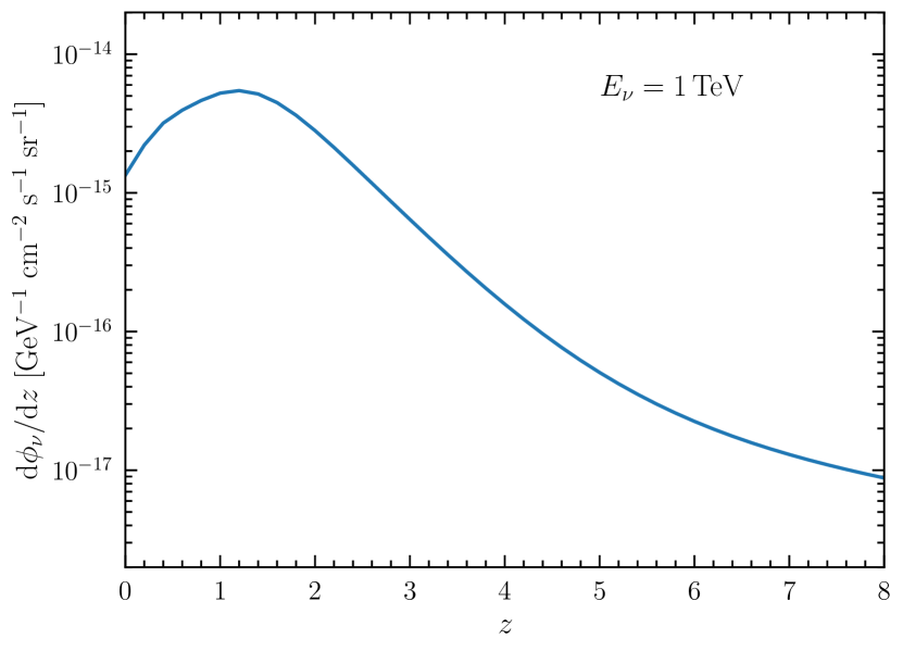
In the left panel of Fig. 7 we show the redshift distribution of the differential flux, once integrated over the luminosity. It represents the neutrino flux coming at different redshift from the sources of all luminosities. The maximum of the distribution stands for $z=1.2$, which represents the maximum of the cosmic star formation rate distribution (Kim et al. 2023). In the left panel of Fig. 7 we show the dependence of the differential flux over $L_{\rm IR}$, integrating over all the redshifts. Hence, it quantifies the contribution from all the sources having a given IR luminosity. We stress that even though the maximum of the differential flux stands for the lowest values of $L_{\rm IR}$, the ULIRGs are the ones which contribute most to the total flux. Indeed, the integration over sources with ${\rm SFR}>100\,M_{\odot}\,{\rm yr^{-1}}(L_{\rm IR}>7.2\cdot 10^{11}\,L_{\odot})$ provides about 58% of the total spectrum. Sources with $1\,M_{\odot}\,{\rm yr^{-1}}<{\rm SFR}<100\,M_{\odot}\,\rm yr^{-1}$ contribute for 38% and the remaining 4% is due to sources with lower star formation rates. Therefore, correctly assessing the calorimetric budget of ULIRGs is fundamental in order to derive correctly the contribution of the entire source population.

Appendix C Impact of the systematic uncertainty on $R_{SN}$

Here we discuss on the impact of the systematic uncertainty on $\rm R_{\rm SN}$. To this purpose, we assume that the systematic uncertainty on $R_{\rm SN}$ is $\sim 45\%$ instead of 20% as adopted in the main analysis. Once summed in quadrature with the $10\%$ uncertainty on the distance, it leads to a systematic error of $50\%$ on $F_{\rm cal}$. Using this systematic error, we perform again the fit of the relation in Eq. (15) and reports the results in Fig. 8.

Figure 8: $F_{\rm cal}$ in terms of $R_{\rm SN}$ for the whole sample. Cyan points denote discovered sources, whereas black points denote undiscovered sources. Specifically, for sources exhibiting a flux compatible with zero, we present 95% CL upper limits indicated by black triangles. For all the sources, $F_{\rm cal}$ and $R_{\rm SN}$values are reported respectively with 50% and 45% systematic uncertainties. We also report the best-fit and the corresponding $1\sigma$ uncertainty band of the fit performed over the whole sample (orange) and over discovered sources (blue).

For the discovered sources, we find $A=1.9\pm 1.1$ and $\beta=0.54\pm 0.11$, while for the combined sample $A=0.5_{-0.2}^{+0.3}$ and $\beta=0.36\pm 0.11$. The fits are totally consistent within the $1\sigma$ with the ones presented in the main text. Furthermore, even though larger uncertainties increase the statistical error of the fits, we still find that undiscovered sources are able to constrain $F_{\rm cal}$ reducing its value especially in the range $[0.2-1]\,\rm yr^{-1}$ at $1\sigma$ level. We emphasise that future measurements will be able to reduce the uncertainty on the supernovae explosion rate and they will provide us with a much more constrained correlation function leading to a smaller uncertainty on the diffuse emissions of SFGs and SBGs.