Light quark mediated Higgs boson production in association with a jet at the next-to-next-leading order and beyond

Abstract

We study the light quark effect on the Higgs boson production in association with a jet at the LHC in the intermediate transverse momentum region between the quark and the Higgs boson mass scales. Though the effect is suppressed by the small Yukawa coupling, it is enhanced by large logarithms of the quark mass ratio to the Higgs boson mass or transverse momentum. Following a remarkable success of the logarithmic expansion Anastasiou:2020vkr for the prediction of the next-to-next-to-leading bottom quark contribution to the total cross section of the Higgs boson production we extend the analysis to its kinematical distributions. A new factorization formula is derived for the light quark mediated $gg\to Hg$ amplitudes and the differential cross section of the process is computed in the logarithmic approximation, which is used for an estimate of the bottom quark effect at the next-to-next-to-leading order.

1 Introduction

Determination of the Higgs boson properties with high precision is a major part of the Large Hadron Collider physics program ATLAS:2016neq ; Cepeda:2019klc . A significant deviation of the measured couplings from the theory predictions may indicate a signal of the physics beyond the standard model. The transverse momentum distribution of the Higgs boson produced in association with a jet is an important kinematical observable sensitive to its Yukawa couplings and can be used to test different extensions of the standard model in different regions of the transverse momentum Arnesen:2008fb ; Bagnaschi:2011tu ; Dawson:2014ora ; Grazzini:2016paz . The dominant contribution to the process cross section is given by the top quark loop mediated gluon fusion. It is known through the next-to-next-to-leading order (NNLO) in the strong coupling constant in the heavy top quark effective theory Chen:2014gva ; Boughezal:2015dra ; Boughezal:2015aha ; Caola:2015wna ; Chen:2016zka and recently has been evaluated to next-to-leading order (NLO) with the full top quark mass dependence Jones:2018hbb . The contribution of the light quarks to the process is strongly suppressed by their masses. This suppression is partially compensated by the enhancement of the leading order amplitude by the second power of the large logarithm $\ln(m_{H}^{2}/m_{q}^{2})$ of the Higgs boson to the light quark mass ratio Baur:1989cm , and the bottom quark effect can be as large as $5\%$ Anastasiou:2016cez . Moreover, the contribution can be distinguished by its transverse momentum dependence for $p_{\perp}\ll m_{H}$, where the cross section is large. This makes the differential distribution sensitive to the light quark Yukawa couplings Bishara:2016jga ; Soreq:2016rae . Thus, it is important to get an accurate prediction for the differential cross section in perturbative QCD. The NLO result in the small quark mass limit has been derived in Lindert:2017pky ; Bonciani:2022jmb . The higher order corrections may also be important due to the presence of the double-logarithmic terms with the second power of the large logarithm per each power of the strong coupling constant. The resummation of the logarithmically enhanced terms poses a serious theoretical challenge for the effective field theory methods Mantler:2012bj ; Grazzini:2013mca ; Banfi:2013eda ; Caola:2018zye due to their non-standard origin Kotsky:1997rq ; Penin:2014msa ; Liu:2017axv . In contrast to the standard Sudakov case Sudakov:1954sw ; Frenkel:1976bj ; Mueller:1979ih ; Collins:1980ih ; Sen:1981sd ; Sterman:1986aj , the logarithmic correction to the mass-suppressed amplitudes are determined by the eikonal color charge nonconservation in the process of the soft quark exchange Liu:2017vkm . The comprehensive analysis of this phenomena in the leading (double) logarithmic approximation has been performed for the three-point amplitudes in QED and QCD Liu:2018czl ; Liu:2021chn . For the four-point amplitudes the abelian part of the all-order result is available for the $gg\to Hg$ production Melnikov:2016emg and only the two-loop result for Bhabha scattering Penin:2016wiw ; Delto:2023kqv . The resummation of the subleading logarithms has been also completed for the $gg\to H$ amplitudes Anastasiou:2020vkr ; Liu:2020wbn ; Liu:2022ajh . The logarithmic expansion turned out to be remarkably successful for the estimate of the bottom quark contribution to the total cross section of the Higgs boson production in the NNLO. The next-to-leading-logarithmic (NLL) approximation for this quantity gives $2.18\pm 0.20~{}pb$ Anastasiou:2020vkr , while the recently computed full result reads $1.99(1)\,{}^{+0.30}_{-0.15}~{}pb$ Czakon:2023kqm . Hence, the generalization of the analysis to the case of the final state jet seems quite important both for general theory of renormalization group at subleading power and from purely phenomenological point of view.

In this paper we extend the abelian result Melnikov:2016emg to the full QCD description of the light quark contribution to the differential cross section of the Higgs boson production in association with a jet for the intermediate values of transverse momentum. This requires a deeper understanding of the origin of the non-Sudakov logarithms and a systematic derivation of the factorization formula. The paper is organized as follows. In the next section we introduce our notations. In Sect. 3 we start with the factorization analysis of the double-logarithmic contribution to the leading order one-loop amplitude, then derive the general all-order resummation formula and compare it to the available two-loop expressions Melnikov:2016qoc . In Sect. 4 we apply this result to the analysis of the $pp\to Hj+X$ differential cross section, which determines the NNLO bottom quark contribution in terms of the known $K$-factors obtained in the heavy quark limit. Sect. 5 is our conclusion.

2 Setup and notations

We consider a light quark mediated Higgs boson production in the process

$$g(p_{1})+g(p_{2})\to g(p_{3})+H(p_{H})$$ (1)

for the intermediate values of the transverse momentum

$$m_{q}^{2}\ll p_{\perp}^{2}\ll s,m_{H}^{2}\,,$$ (2)

where $p_{\perp}^{2}=ut/s$, $s=(p_{1}+p_{2})^{2},t=(p_{1}-p_{3})^{2},u=(p_{2}-p_{3})^{2}$. We focus on the near-threshold production for partonic center-of-mass energy $s\approx m_{H}^{2}$ so that the additional soft gluon emission energy is small compared to the leading jet. This, in particular, means that the transverse momenta of the Higgs boson and the jet are approximately equal in magnitude. The above kinematical region gives the dominant contribution to the hadronic cross section. For $p_{\perp}^{2}\ll s$ the process is described by four helicity amplitudes $M_{\lambda_{1}\lambda_{2}\lambda_{3}}$ with the same helicity of colliding gluons $\lambda_{1}=\lambda_{2}$, which are pairwise connected by spatial inversion. We take $M_{++\pm}$ as the two independent amplitudes and only keep the leading terms which grow as $1/p_{\perp}$ with decreasing transverse momentum. In the spinor notations the corresponding expressions read

$$M_{+++} = -\sqrt{2}f^{a_{1}a_{2}a_{3}}{g_{s}\over v}\frac{\alpha_{s}}{4\pi}\frac{\langle 12\rangle^{2}}{[12]\langle 23\rangle\langle 13\rangle}Z_{3g}\sum_{q}A_{+++}^{(q)}\,,$$ (3)

$$M_{++-} = -\sqrt{2}f^{a_{1}a_{2}a_{3}}{g_{s}\over v}\frac{\alpha_{s}}{4\pi}\frac{\langle 12\rangle}{[23][13]}Z_{3g}\sum_{q}A_{++-}^{(q)}\,,$$ (4)

where $\alpha_{s}=g_{s}^{2}/(4\pi)$ is the strong coupling constant, $v$ is the Higgs field vacuum expectation value, $f^{a_{1}a_{2}a_{3}}$ is the $SU(3)$ structure constant, the sum goes over the quark flavors, $Z_{3g}$ is the Sudakov factor incorporating the soft and collinear divergences of the amplitudes, and $A_{++-}^{(q)}$ are the infrared finite form factors. Let us first discuss the leading contribution of the top quark which can be expanded in the inverse powers of $m_{t}$. The perturbative series for the form factors then take the following form

$$A_{++\pm}^{(t)}=C_{t}\sum_{n=0}\left({\alpha_{s}\over 2\pi}\right)^{n}\tilde{A}^{(n)}_{++\pm}+{\cal O}(m_{t}^{-2})\,,$$ (5)

where the Wilson coefficient $C_{t}=1+{11\over 4}{\alpha_{s}\over\pi}+\ldots$ is known through $\alpha_{s}^{4}$ Schroder:2005hy ; Chetyrkin:2005ia , $\tilde{A}^{(0)}_{++\pm}=\pm{2/3}$, and $\tilde{A}^{(n)}_{++\pm}$ stands for the $n$-loop correction computed in the heavy top effective theory, which is available up to $n=2$ Gehrmann:2011aa . For light quarks the amplitudes can be expanded in powers of $m_{q}$ and the perturbative series for the form factors reads

$$A_{++\pm}^{(q)}={m_{q}^{2}\over s}\sum_{n=0}\left({\alpha_{s}\over 2\pi}\right)^{n}A^{(n+1)}_{++\pm}+{\cal O}(m_{q}^{4})\,,$$ (6)

where $A^{(n)}_{++\pm}$ stands for the $n$-loop QCD contribution also available up to $n=2$ Melnikov:2016qoc . These coefficients include the terms enhanced by the large logarithms of the scale ratios $p_{\perp}^{2}/m_{q}^{2}$, $m_{H}^{2}/m_{q}^{2}$ or $t/u$, which becomes relevant at large rapidity. The goal of this work is to compute the coefficients $A^{(n)}_{++\pm}$ in the leading (double) logarithmic approximation, i.e. keeping the highest power of the large logarithms equal to $2n$, for all $n$.

In the leading logarithmic approximation the Sudakov factor can be written as follows $Z^{LL}_{3g}=e^{{\alpha_{s}\over 2\pi}I^{(1)}}$ where $I^{(1)}$ is an analog of the one-loop Catani’s operator Catani:1998bh with the trivial structure in the color space. It is a function of the Mandelstam variables and is scheme dependent. To make the factorization of the Sudakov and non-Sudakov logarithms explicit it is convenient to define this function in such a way that it incorporates the nonsingular double logarithmic dependence of the one-loop corrections to the effective theory amplitudes with the local $ggH$ interaction on the kinematical invariants. By using the result Schmidt:1997wr it is straightforward to get the leading singularity subtraction operator in the “physical” scheme

$$I^{(1)}_{\rm ph}=-{C_{A}\over 2\epsilon^{2}}\left[2\left({-s\over\mu^{2}}\right)^{-\epsilon}+\left({-tu\over s\mu^{2}}\right)^{-\epsilon}\right],$$ (7)

where $\epsilon=2-d/2$ is the parameter of dimensional regularization and $C_{A}=N_{c}$ for the $SU(N_{c})$ color gauge group. Note that the canonical symmetric form of the subtraction operator has been used in Melnikov:2016qoc , which differs from Eq. (7) by a non-singular double logarithmic terms, as discussed in Sect. 3.2.

3 Factorization and resummation of the leading logarithms

3.1 Factorization of the one-loop amplitudes

$1$ $2$            $3$
(a)	(b)	(c)

Figure 1: One-loop diagrams representing the leading order light quark contribution to $gg\to Hg$ process. Wide and narrow gluon lines correspond to the initial and final gluon states, respectively. Symmetric diagrams corresponding to the opposite direction of the quark flow and to the soft emissions off the opposite gluon/quark line are not shown. In the first diagram the gluons are explicitly enumerated according to their momentum index.

A detailed discussion of the evaluation of the leading order one-loop amplitude in the double-logarithmic approximation can be found in Melnikov:2016emg . It, however, does not reveal a deeper factorization structure, which is crucial for the full QCD analysis and is discussed in this section. Following Melnikov:2016emg we choose the gluon polarization vectors $\epsilon_{i}$ satisfying the gauge conditions

$$\epsilon_{i}p_{i}=0\quad(i=1,2,3)\,,\qquad\epsilon_{1}p_{2}=0\,,\qquad\epsilon_{2}p_{1}=0\,,\qquad\epsilon_{3}p_{2}=0\,,$$ (8)

so that the jet cannot be emitted off the gluon or quark line carrying the large light-cone momentum $p_{2}$. It is convenient to choose a frame where the light-cone components ${p_{1}}_{\perp}={p_{2}}_{\perp}=p_{1}^{+}=p_{2}^{-}=\epsilon_{3}^{-}=0$. Then, up to the direction of the closed quark line the leading order process is described by the three diagrams in Fig. 1. The diagrams Fig. 1(a,b) have the standard structure of soft emission from a highly energetic eikonal line. In the diagram Fig. 1(c), however, the jet is emitted from the soft quark line which does not carry the large momenta $p_{1,2}$. We focus on the specific structure of the corresponding double logarithmic contribution. Due to the helicity conservation in the small mass limit and the helicity flipping scalar Yukawa interaction, the light quark contribution is mass suppressed. The mass-suppressed double-logarithmic corrections are known to be generated by the on-shell soft quark contribution. Thus the quark propagator in the expression for the Feynman diagrams in Fig. 1 can be approximated as follows

$$S(l)\equiv{1\over/{l}-m_{q}+i0}\to-im_{q}\pi\delta(l^{2}-m_{q}^{2})\,,$$ (9)

where $l$ is the soft loop momentum and the mass factor accounts for the required helicity flip on the virtual quark line.

Each of the two t-channel quark propagators in Fig. 1(c) can go on-shell which defines two soft virtual momentum regions. Let us consider the one with the upper on-shell propagator so that the jet momentum $p_{3}$ flows through the lower one. After omitting irrelevant terms, the off-shell quark propagators become

$$S(p_{1}+l)\to\frac{/{p_{1}}}{2p_{1}l}\,,$$ (10)

$$S(p_{3}+l)\to\frac{/{p_{3}}+/{l}}{2p_{3}l}\,,$$ (11)

$$S(p_{3}-p_{2}+l)\to\frac{/{p_{2}}}{2p_{2}p_{3}+2p_{2}l}\,.$$ (12)

Then the integral develops the double logarithmic scaling either with the first term in the numerator of Eq. (11) for $|p_{2}l|<|p_{2}p_{3}|$ or with the second term for $|p_{2}p_{3}|<|p_{2}l|$. Thus we can write

$$S(p_{3}+l)/{\epsilon_{2}}S(p_{3}-p_{2}+l) \to \theta\left(|p_{2}p_{3}|-|p_{2}l|\right){/{p_{3}}\over 2p_{3}l}/{\epsilon_{2}}{/{p_{2}}\over 2p_{2}p_{3}}$$ (13)

$$+\theta(|p_{2}l|-|p_{2}p_{3}|){/{l}\over 2p_{3}l}/{\epsilon_{2}}{/{p_{2}}\over 2p_{2}l}\,.$$

This decomposition, however, does not reflect the factorization structure in the effective theory terms and we rewrite it as follows

$$S(p_{3}+l)/{\epsilon_{2}}S(p_{3}-p_{2}+l) \to \theta\left(|p_{2}p_{3}|-|p_{2}l|\right)\left({/{p_{3}}\over 2p_{3}l}/{\epsilon_{2}}{/{p_{2}}\over 2p_{2}p_{3}}-{/{l}\over 2p_{3}l}/{\epsilon_{2}}{/{p_{2}}\over 2p_{2}l}\right)$$ (14)

$$+{/{l}\over 2p_{3}l}/{\epsilon_{2}}{/{p_{2}}\over 2p_{2}l}\,,$$

where the integration region is extended in the second term and its variation is subtracted from the first term.

Let us first consider the contribution proportional to the theta-function in Eq. (14). It includes two distinct structures corresponding to two terms in the brackets. For the second term in the logarithmic integration region ${/{\,l}\over 2p_{3}l}$ can be replaced by ${/{p_{1}}\over 2p_{3}p_{1}}$, which results in the amplitude proportional to $\epsilon_{3}p_{1}\over p_{3}p_{1}$ characteristic to the color-dipole emission from the eikonal line of the momentum $p_{1}$, and gives $A_{+++}=-A_{++-}$. Moreover, the only dependence on the momentum $p_{3}$ is through the argument of the theta-function and the integrand coincides with the one of the one-loop $ggH$ amplitude. Thus this soft dipole contribution reduces to the effective diagram Fig. 2(a) with the decoupled jet and a constraint $|p_{2}l|<|p_{2}p_{3}|$ on the loop momentum. The double line in this diagram stands for the eikonal (Wilson) line defined by the light-like momentum $p_{1}$, with the propagator $-p_{1}/(2p_{3}p_{1})$. The calculation of this contribution is straightforward by using the classical Sudakov technique which converts the integral over $l$ into the integral over the logarithmic Sudakov variables $\eta=\ln(|lp_{3}|/|p_{1}p_{3}|)/L$ and $\xi=\ln(|lp_{1}|/|p_{2}p_{1}|)/L$ (see Melnikov:2016emg for the details)

$$\left[A^{(1)}_{++\pm}\right]_{\rm s.d.}=\mp L^{2}\int_{\tau_{t}-\tau}^{\tau_{t}}{\rm d}\eta\int_{1-\tau_{t}}^{1-\eta}{\rm d}\xi=\mp{L^{2}}{\tau^{2}\over 2}\,,$$ (15)

where $L=\ln(s/m_{q}^{2})$, $\tau_{t}=\ln\left({|t|/m_{q}^{2}}\right)/L$, and $\tau=\ln\left({p_{\perp}^{2}/m_{q}^{2}}\right)/L$. Note that a dipole contribution from the virtual momentum configuration where the lower t-channel propagator goes on-shell and the jet momentum $p_{3}$ flows through the upper one is proportional to $\epsilon_{3}p_{2}$ and vanishes for our gauge condition.

(a)	(b)	(c)

Figure 2: The effective representation of the sum of the one-loop diagrams in Fig. 1 after decomposition into the dipole and symmetric structures. The double line represents the eikonal line defined by the momentum $p_{1}$, as explained in the text. The black circle corresponds to the effective vertex.

The first term in the brackets in Eq. (14) proportional to $p_{3}$ results in a new symmetric tensor structure described by a gauge invariant operator $G_{\mu\nu}^{a}G^{b}_{\nu\lambda}G_{\lambda\mu}^{c}f^{abc}$, which does not contribute to the all-plus helicity amplitude. It can be represented by the effective theory diagram Fig. 2(a) with the propagator $S(p_{2}-p_{3}+l)$ collapsed to an effective local vertex. Due to its symmetry and explicit gauge invariance this structure does get the equal contribution from the crossing-symmetric configuration with the opposite direction of the jet momentum flow represented by the effective diagram in Fig. 2(b). The sum gives the symmetric contribution

$$\left[A^{(1)}_{++-}\right]_{\rm sym.}=-L^{2}\left(\int_{\tau_{t}-\tau}^{\tau_{t}}{\rm d}\eta\int_{1-\tau_{t}}^{1-\eta}{\rm d}\xi+(\tau_{t}\leftrightarrow\tau_{u})\right)=-{L^{2}}{\tau^{2}}\,,$$ (16)

where $\tau_{u}=\ln\left({|u|/m_{q}^{2}}\right)/L$. The total contribution of the theta-function term then reads

$$\left[A^{(1)}_{++\pm}\right]_{\rm s.d.}+\left[A^{(1)}_{++\pm}\right]_{\rm sym.}=-{\tau^{2}\over 2}L^{2}\,.$$ (17)

It is helicity independent and vanishes at the boundary of the transverse momentum region $p_{\perp}\to m_{q}$ where $\tau\to 0$.

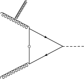
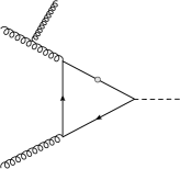
$\mbox{\boldmath$\to$}~{}{1\over 2}$	$\mbox{\boldmath$\to$}~{}{1\over 2}$	$\to$
(a)	(b)	(c)	(d)

Figure 3: Diagrammatic representation of the sequence of the Ward identities and momentum shifts which relates the unconstrained dipole contribution of the diagram Fig. 1(c) to the diagram Fig. 1(b), as explained in the text. The empty circle marks the subtracted quark propagator.

To account for the unconstrained dipole contribution of the second line in Eq. (14) we use the method of Liu:2018czl and move the jet vertex from the soft quark propagator to the eikonal line, Fig 3. This can be done in three steps. First we transform the soft line as follows

$$S(l)/{\epsilon_{3}}S(l+p_{3})=S(l)/{\epsilon_{3}}S(l+p_{3}^{+})+\ldots={\epsilon_{3}p_{1}\over p_{3}p_{1}}\left(S(l)-S(l+p_{3}^{+})\right)+\ldots\,,$$ (18)

where we used the fact that $\epsilon_{3}^{-}=0$, and the omitted terms do not contribute to the leading logarithms. This transformation, being a particular realization of the Slavnov-Ward identities, is graphically represented by the diagram Fig. 3(b), where the empty circle on the quark propagator represents the replacement $S(l)\to S(l)-S(l+p_{3}^{+})$ and the factor $1/2$ comes from the color weight of the diagrams. By the momentum shift $l\to l-p_{3}^{+}$ in the second term of the above expression the crossed circle can be moved to the upper eikonal quark line which becomes $S(p_{2}+l)-S(p_{2}+l-p_{3}^{+})$, Fig. 3(c). The opposite eikonal line is not sensitive to this shift since $p_{2}^{-}=0$. On the final step we use the “inverted identity” on the upper eikonal quark line

$${\epsilon_{3}p_{1}\over p_{3}p_{1}}\left(S(p_{2}+l)-S(p_{2}+l-p_{3}^{+})\right)=-S(p_{2}+l)/{\epsilon_{3}}S(p_{2}+l-p_{3})+\ldots\,,$$ (19)

to transform the diagram Fig. 2(c) into Fig. 2(d) equal to Fig. 1(b). Now we can combine this dipole part of the diagram Fig. 1(c) with the diagrams Fig. 1(a,b) to get the standard eikonal factorization Fig. 1(a)$+$2 Fig. 1(b)$=$ Fig. 2(a) where the factor 2 accounts for the difference in the color weights. In Fig. 2(a) the jet is emitted by the eikonal Wilson line of momentum $p_{1}$ and is completely decoupled from the quark loop without the constraint on the loop momentum present in the soft dipole contribution. Thus this eikonal dipole contribution reduces to the one-loop $g(p_{1})g(p_{2})H$ form factor

$$\left[A^{(1)}_{++\pm}\right]_{\rm e.d.}=\pm 2L^{2}\int_{0}^{1}{\rm d}\eta\int_{0}^{1-\eta}{\rm d}\xi=\pm L^{2}\,,$$ (20)

and is independent of the jet kinematics. By adding up Eqs. (17) and (20) we get

$$A^{(1)}_{+++}=L^{2}\left(1-{\tau^{2}\over 2}\right),\qquad A^{(1)}_{++-}=-L^{2}\left(1+{\tau^{2}\over 2}\right),$$ (21)

in agreement with Baur:1989cm .

The main result of this section is the decomposition of the one-loop amplitudes into the eikonal dipole, soft dipole, and symmetric parts. In the first one the jet emission factors out from the quark loop, as it happens for $p_{\perp}\ll m_{q}$, i.e. in the heavy quark limit with the effective $g(p_{1})g(p_{2})H$ vertex. The last two describe the deviation from this factorization, accommodate all the dependence on the jet kinematical variables, and vanish when $p_{\perp}\to m_{q}$. The soft dipole contribution reduces to the quark-loop mediated $g(p_{1})g(p_{2})H$ form factor with a new ultraviolet constraint on the double logarithmic region of loop momentum depending on jet kinematics. The symmetric contribution is characterized by a new local effective vertex involving one of the initial state gluons and reduces to the quark-loop mediated $g(p_{3})g(p_{1,2})H$ form factors with one of the gluons being the jet and with the same constraint on the double logarithmic region.

3.2 All-order analysis

(a)	(b)	(c)
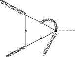
(d)	(e)	(f)

Figure 4: (a,b,c) Factorization of the soft interaction of the initial state gluon in the symmetric contribution. The eikonal double line carries the jet momentum. (d) The factorized soft interaction of the final state gluon in the dipole contribution. The eikonal double line carries the initial state momentum. (e) The heavy quark limit diagram with the same structure of the infrared Sudakov logarithms as the diagrams (c) and (d). (f) The Sudakov-Wilson contribution with the soft gluon momentum resolving the collapsed propagator. The empty circle represents the dipole interaction with the adjusted color weight.

The result of the previous section makes the all-order resummation of the double logarithmic radiative corrections rather straightforward. These corrections are generated by the soft virtual gluons with the well known factorization and exponentiation properties Sudakov:1954sw ; Frenkel:1976bj which should be adjusted to account for the non-Sudakov logarithms in the soft quark initiated processes Liu:2017vkm ; Liu:2018czl . The latter are characteristic to the interaction of the eikonal lines connected by the soft quark. Thus we do not expect the non-Sudakov contribution from the interaction of the decoupled gluons to the quark loop. An example of the eikonal factorization of this interaction for the symmetric contribution is shown in Fig. 4. If the soft gluon momentum does not resolve the local vertex we have Fig. 4(a)$+$Fig. 4(b)$=$Fig. 4(c). Note that the interaction of the virtual gluon with the soft quark has the vanishing color factor. For the dipole contribution similar factorization results in the diagram Fig. 4(d). Both diagrams Fig. 4(c,d) have the same structure of the Sudakov logarithms as the effective theory diagram Fig. 4(e) with the local $g(p_{1})g(p_{2})H$ vertex. Hence with our definition of the operator $I^{(1)}_{\rm ph}$ all the corresponding singular and finite double logarithmic terms are included in $Z_{3g}$ factor and we are left with the soft corrections to a quark loop mediated $ggH$ amplitude, where one of the gluon can be the jet. The structure of the double-logarithmic corrections to such an amplitude is well understood too. In general, after factoring out Sudakov corrections absorbed into $Z_{3g}$ we get the non-Sudakov double logarithmic contribution associated with $A_{++\pm}$. The structure of the factorization and the non-Sudakov logarithms, however, is different for the dipole and symmetric contributions. Let us first discuss the eikonal dipole part of the result. In this case the jet completely decouples from the quark loop and one can use the result Liu:2017vkm ; Liu:2018czl for the $g(p_{1})g(p_{2})H$ amplitude, which gives

$$\left[A_{++\pm}^{\rm LL}\right]_{\rm e.d.}=\pm 2L^{2}\int_{0}^{1}{\rm d}\eta\int_{0}^{1-\eta}{\rm d}\xi\,e^{2z\eta\xi}=\pm L^{2}\int_{0}^{1}{{\rm d}\eta\over z\eta}\left(e^{2z\eta(1-\eta)}-1\right)=\pm L^{2}g(z)\,,$$ (22)

where $g(z)={}_{2}F_{2}\left(1,1;{3/2},2;{z/2}\right)$ is the hypergeometric function, $z=(C_{A}-C_{F})x$, $C_{F}={N_{c}^{2}-1\over 2N_{c}}$, and $x=\frac{\alpha_{s}(\mu_{s})}{4\pi}L^{2}$. The exponent $e^{2z\eta\xi}$ in Eq. (22) is the off-shell $\bar{q}qH$ Sudakov form factor with the color weight $C_{F}$ replaced by $C_{F}-C_{A}$ accounting for the variation of the color group representation for a particle moving along the eikonal lines from adjoint to fundamental in the process of the soft quark emission, which is the physical origin of the non-Sudakov logarithms.

The soft dipole contribution differs from the eikonal one by the cutoff of the double-logarithmic region of virtual momentum. This is an ultraviolet cutoff which does not change the infrared structure of the factorization and therefore can be imposed directly in Eq. (22). This gives

$$\left[A_{++\pm}^{\rm LL}\right]_{\rm s.d.}=\mp L^{2}\int_{\tau_{t}-\tau}^{\tau_{t}}{\rm d}\eta\int_{1-\tau_{t}}^{1-\eta}{\rm d}\xi\,e^{2z\eta\xi}=\mp L^{2}\int_{\tau_{t}-\tau}^{\tau_{t}}{{\rm d}\eta\over 2z\eta}\left(e^{2z\eta(1-\eta)}-e^{2z\eta(1-\tau_{t})}\right)\,,$$ (23)

cf. Eqs. (15, 20).

For the symmetric contribution the eikonal lines carry the momenta $p_{3}$ and $p_{1}$ or $p_{2}$. Thus for i.e. $g(p_{1})g(p_{3})H$ amplitude the exponential factor of Eq. (22) should be changed to $e^{2z(\eta-\tau_{t}+\tau)(\xi-1+\tau_{t})}$, while the integration limits are the same as in Eq. (23). However, if a light-cone component of the virtual soft gluon momentum exceeds the one of $p_{3}$, it may resolve the local effective vertex and such a correction is not taken into account by the above exponent. In this case the jet becomes soft with respect to the virtual gluon momentum and factors out of the corresponding loop integral. Thus, the factorization of the Sudakov corrections is realized in the same way as for the $g(p_{1})g(p_{2})H$ amplitude. The resulting non-Sudakov contribution is accounted for by introducing a “Sudakov-Wilson” factor $e^{2z(\tau_{t}-\tau)\xi}$ local along one of the eikonal lines, Fig. 4(f), with the adjusted $C_{F}-C_{A}$ color weight. Compared to Eq. (22), in this expression the $\tau_{t}-\tau$ factor replaces the logarithmic variable $\eta$ as the infrared cutoff for the collapsed quark propagator in the effective vertex. Combining the corrections we get

$$\left[A_{++-}^{\rm LL}\right]_{\rm sym.} = -L^{2}\left[\int_{\tau_{t}-\tau}^{\tau_{t}}{\rm d}\eta\int_{1-\tau_{t}}^{1-\eta}{\rm d}\xi\,e^{2z(\eta-\tau_{t}+\tau)(\xi-1+\tau_{t})}e^{2z(\tau_{t}-\tau)\xi}+(\tau_{t}\to\tau_{u})\right]$$ (24)

$$= -L^{2}\left[\int_{\tau_{t}-\tau}^{\tau_{t}}{{\rm d}\eta\over 2z\eta}e^{2z(\tau_{t}-\tau)(1-\tau_{t})}\left(e^{2z\eta(\tau_{t}-\eta)}-1\right)+(\tau_{t}\to\tau_{u})\right].$$

Thus the effective theory decomposition of the symmetric contribution has a more complex structure with the short-distance effects described by the Sudakov-Wilson factor.

We have verified the above factorization structure of the amplitudes by explicit identification and evaluation of the double-logarithmic contributions to the two-loop diagrams using the technique Liu:2018czl .

The total all-order leading logarithmic approximation for the helicity form factors can be written in a compact form

$$A_{+++}^{LL} = L^{2}\bigg{[}g(z)-\int_{(1-\tau+\zeta)/2}^{(1+\tau+\zeta)/2}{{\rm d}\eta\over 2z\eta}\left(e^{2z\eta(1-\eta)}-e^{z\eta(1-\tau-\zeta))}\right)\bigg{]},$$ (25)

$$A_{++-}^{LL} = -A_{+++}^{LL}-L^{2}\bigg{[}\int_{(1-\tau+\zeta)/2}^{(1+\tau+\zeta)/2}{{\rm d}\eta\over 2z\eta}\,e^{z((1-\tau)^{2}-\zeta^{2})/2}\left(e^{z\eta(1+\tau+\zeta-2\eta)}-1\right)+(\zeta\to-\zeta)\bigg{]},$$

where $\zeta=\ln(t/u)/L$ is the rapidity variable. At the boundary values of the allowed transverse momentum interval Eqs. (25, LABEL:eq::fullLLm) simplify and can be obtained in a closed analytic form. For $p_{\perp}\to m_{b}$ corresponding to $\tau\to 0$ the soft dipole and symmetric contributions vanish and we get

$$A_{++\pm}^{LL}|_{\tau=0}=\pm L^{2}g(z)\,.$$ (27)

At the same time for central rapidity $\zeta=0$ and $p_{\perp}\to m_{H}$ corresponding to $\tau\to 1$ we have $|s|\sim|t|\sim|u|$ and up to an overall factor the symmetric, soft and eikonal dipole contributions are determined by the same $ggH$ form factor. This gives

$$A_{+++}^{LL}|_{\tau=1,\,\zeta=0}={1\over 2}L^{2}{g(z)}\,,\qquad A_{++-}^{LL}|_{\tau=1,\,\zeta=0}=-{3\over 2}L^{2}{g(z)}\,.$$ (28)

By expanding Eqs. (25, LABEL:eq::fullLLm) in $z$ we get the two-loop amplitudes

$$A_{+++}^{(2)} = {(C_{A}-C_{F})L^{4}\over 24}\left(2-{3\tau^{2}}+{2\tau^{3}}+{3\tau^{2}\zeta^{2}}\right),$$ (29)

$$A_{++-}^{(2)} = -{(C_{A}-C_{F})L^{4}\over 24}\left(2+{3\tau^{2}}-{6\tau^{3}}+{4\tau^{4}}-{3\tau^{2}\zeta^{2}}\right),$$ (30)

which can be compared to the result of the explicit calculation Melnikov:2016qoc . The comparison, however, is not straightforward since in Melnikov:2016qoc the canonical symmetric form of the Catani’s operator has been adopted

$$I^{(1)}_{\rm sym}=-{C_{A}\over 2\epsilon^{2}}\left[\left({-s\over\mu^{2}}\right)^{-\epsilon}+\left({-t\over\mu^{2}}\right)^{-\epsilon}+\left({-u\over\mu^{2}}\right)^{-\epsilon}\right],$$ (31)

which differs from Eq. (7) by

$$\delta I^{(1)}=-{C_{A}\over 8}L^{2}\left[\left(1-\tau\right)^{2}-\zeta^{2}\right].$$ (32)

Thus for the helicity form factors defined in Melnikov:2016qoc we need to perform the infrared matching Penin:2005kf ; Penin:2005eh

$$\bar{\Omega}_{+++}^{(2l),{\rm fin}}=A_{+++}^{(2)}+\delta I^{(1)}A_{+++}^{(1)}\,,\qquad-\bar{\Omega}_{++-}^{(2l),{\rm fin}}=A_{++-}^{(2)}+\delta I^{(1)}A_{++-}^{(1)}\,,$$ (33)

which gives

$$\bar{\Omega}_{+++}^{(2l),{\rm fin}} = -{L^{4}\over 24}\left[C_{A}+2C_{F}-6C_{A}\tau+\left({9\over 2}C_{A}-3C_{F}\right){\tau^{2}}+\left(C_{A}+2C_{F}\right){\tau^{3}}\right.$$ (34)

$$\left.-3C_{A}\zeta^{2}+\left(-{3\over 2}C_{A}+3C_{F}\right)\tau^{2}\zeta^{2}\right],$$

$$\bar{\Omega}_{++-}^{(2l),{\rm fin}} = -{L^{4}\over 24}\left[C_{A}+2C_{F}-6C_{A}\tau+\left({3\over 2}C_{A}+3C_{F}\right){\tau^{2}}+\left(3C_{A}+6C_{F}\right){\tau^{3}}\right.$$ (35)

$$\left.+\left(-{5\over 2}C_{A}+4C_{F}\right)\tau^{4}-3C_{A}\zeta^{2}+\left({3\over 2}C_{A}-3C_{F}\right)\tau^{2}\zeta^{2}\right].$$

Upon changing the notations $\zeta\to\xi$, $\tau\to-\tau$, for $C_{A}=3$, $C_{F}=4/3$, Eqs. (34, 35) agree with Eqs. (6.11, 6.12) of Melnikov:2016qoc , providing a nontrivial check of our analysis. Note that for the symmetric choice of the infrared subtraction the physical $C_{F}-C_{A}$ color scaling is missing.

4 Logarithmic corrections to the kinematical distributions

We now can apply the result of the previous section to estimate the bottom quark effect to the differential cross section of the Higgs boson production in association with a jet. The dominant contribution is due to the interference of the top and bottom quark mediated amplitudes. We discard the partonic channel with the initial state quarks and consider the numerically dominant contribution of the gluon fusion. In the physical inclusive cross section the processes with additional real emission should be taken into account. If the real emission energy $E_{\rm real}$ exceeds $m_{b}$, it resolves the bottom quark loop and may generate a new type of the double logarithms. We, however, treat all the real emission as in the heavy quark limit with the local $ggH$ interaction. This approximation is discussed at the end of the section. Then both the virtual Sudakov and the soft real corrections are the same in the bottom and top quark mediated processes and the correction to the differential partonic cross section can be written as follows

$$d\sigma^{tb}_{gg\to Hg+X}=-\frac{3m_{b}^{2}}{m_{H}^{2}}L^{2}C_{t}C_{b}(\tau,\zeta)d\tilde{\sigma}^{\rm eff}_{gg\to Hg+X}\,.$$ (36)

where $d\tilde{\sigma}^{\rm eff}_{gg\to Hg+X}$ is computed in the heavy top effective theory and

$$C_{b}(\tau,\zeta) = {A_{+++}-A_{++-}\over 2L^{2}}=1+{z\over 6}\left(1-\tau^{3}+\tau^{4}\right)$$ (37)

$$+ {z^{2}}\left[{1\over 45}-{\tau^{3}\over 12}+{\tau^{4}\over 6}-{7\tau^{5}\over 60}+{\tau^{6}\over 30}+{\zeta^{2}\over 12}(\tau^{3}-\tau^{4})\right]$$

$$+ {z^{3}}\left[{1\over 420}-{\tau^{3}\over 48}+{\tau^{4}\over 16}-{\tau^{5}\over 12}+{23\tau^{6}\over 360}-{143\tau^{7}\over 5040}+{31\tau^{8}\over 5040}\right.$$

$$+ \left.{\zeta^{2}}\left({\tau^{3}\over 24}-{\tau^{4}\over 12}+{\tau^{5}\over 20}-{\tau^{6}\over 180}\right)-{\zeta^{4}\over 48}(\tau^{3}-\tau^{4})\right]+\ldots$$

is a function of the transverse momentum and rapidity. Convolution of Eq. (36) with the parton distribution functions gives the correction to the kinematical distributions of the $pp\to Hj+X$ production in the threshold approximation.

However, within a well-motivated approximation the analysis of the hadronic cross section can be significantly simplified Melnikov:2016emg . Indeed, the dependence of Eq. (37) on the jet rapidity is very weak. It starts with ${\cal O}(z^{2})$ and the rapidity-dependent terms include at least the second power of the variable $\zeta$ and the third power of the variable $\tau$. If the soft jet is emitted at large rapidity, we have $|\zeta|\approx 1$ and $\tau\ll 1$. On the contrary, central emission with the large transverse momentum implies $|\zeta|\ll 1$ and $\tau\approx 1$. Therefore, the rapidity-dependent terms are small everywhere and can be neglected. Then $C_{b}(\tau,0)$ factors out from the parton distribution function integral. At the same time the transverse momentum dependence of the coefficients in Eq. (37) turned out to be very weak too, Fig. 5, and it can be approximated by $C_{b}=C_{b}(0,\zeta)=C_{b}(1,0)$ with a very high accuracy. This is quite a nontrivilal fact since the individual helicity form factors strongly depend on the transverse momentum, Eqs. (27, 28). The coefficient $C_{b}=1+\sum_{n=1}^{\infty}c_{n}$ is saturated by the eikonal dipole part of the factorization formula with the jet emission decoupled from the quark loop and describes the non-Sudakov logarithmic corrections to the total cross section of the Higgs boson production. It is known through the NLL approximation Anastasiou:2020vkr . The first three terms of the series read

$$c_{1} = {z\over 6}+C_{F}{\alpha_{s}L\over 4\pi}\,,$$

$$c_{2} = {z^{2}\over 45}+{x\over 5}{\alpha_{s}L\over 4\pi}\left[{3\over 2}C_{F}-\beta_{0}\left({5\over 6}{L_{\mu}\over L}-{1\over 3}\right)\right],$$ (38)

$$c_{3} = {z^{3}\over 420}+{x^{2}\over 5}{\alpha_{s}L\over 4\pi}\left[{5\over 21}C_{F}-\beta_{0}\left({2\over 9}{L_{\mu}\over L}-{2\over 21}\right)\right],$$

where $\beta_{0}={11\over 3}C_{A}-{4\over 3}T_{F}n_{l}$, $n_{l}=5$, $L_{\mu}=\ln(s/\mu^{2})$ and $\mu$ is the renormalization scale of $\alpha_{s}$ in the double-logarithmic variable $z$. Thus neglecting the tiny soft dipole and symmetric contributions to the factorization formula we can extend the NLL analysis of the total threshold cross section to the process with the final jet. This gives

$${d\sigma^{tb}_{pp\to Hj+X}}=-\frac{3m_{b}^{2}}{m_{H}^{2}}\left({\alpha_{s}(m_{H})\over\alpha_{s}(m_{b})}\right)^{\gamma_{m}^{(1)}/\beta_{0}}L^{2}{C_{b}C_{t}}{d\tilde{\sigma}^{\rm eff}_{pp\to Hj+X}}\,,$$ (39)

where $\gamma^{(1)}_{m}={3}C_{F}$ is the one-loop mass anomalous dimension and the renormalization group factor sets the physical scale of the bottom quark Yukawa coupling to $m_{H}$. Clearly, in this approximation we miss the NLL terms in $C_{b}(\tau,\zeta)$ with the non-trivial dependence on the kinematical variables. However, the analysis of the total cross section Anastasiou:2020vkr indicates that the main effect of the non-Sudakov NLL contribution is in fixing the physical renormalization scales of the strong and Yukawa couplings in the leading-logarithmic result, which is included into Eq. (39).

It is instructive to rewrite this formula in a way which relates the $K$-factors for the top-bottom interference contribution and the top quark mediated cross section in the heavy top limit

$${d\sigma^{tb}_{pp\to Hj+X}}=\left[{C_{b}\over C_{t}}\left({\alpha_{s}(m_{H})\over\alpha_{s}(m_{b})}\right)^{\gamma_{m}^{(1)}/\beta_{0}}\right]\left({d\sigma^{tb}_{pp\to Hj+X}\over d\sigma^{tt}_{pp\to Hj+X}}\right)^{\rm LO}{d\sigma^{tt}_{pp\to Hj+X}}\,.$$ (40)

Here the first factor accounts for the difference between the QCD corrections to the top and bottom quark contributions. In the above approximation this difference does not depend on the kinematical variables and does not exceed twenty percent in the NLO, in agreement with the full calculation Lindert:2017pky . The NNLO term in the expansion of this factor amounts of a few percent so that the total NNLO correction to the bottom quark contribution is dominated by the K-factor of the top quark mediated cross section Chen:2014gva ; Boughezal:2015dra ; Boughezal:2015aha ; Caola:2015wna ; Chen:2016zka . Note that in the NLL approximation there is no difference between the pole mass $m_{b}$ and the $\overline{\rm MS}$ mass $\bar{m}_{b}(\bar{m}_{b})$ but the use of the latter as the bottom quark mass parameter in the available exact fixed order results Anastasiou:2020vkr boosts the convergence of the perturbative expansion (cf. Czakon:2023kqm ).

An important property of our result is that at $p_{\perp}\to m_{b}$ the soft dipole and symmetric parts of the factorization formula vanish and in the remaining eikonal part the jet is completely decoupled from the quark loop. Thus, the transverse momentum evolution of the cross section matches the one for $p_{\perp}\ll m_{b}$ derived in the heavy bottom effective theory with $C_{b}$ playing the role of the Wilson coefficient of the local $ggH$ interaction. Moreover, up to a tiny corrections even for $m_{q}\ll p_{\perp}$ the jet emission factors out as in the large quark mass limit. We may assume a similar behavior of the unresolved real emission with the energy below the energy of the jet. Then our result, being formally valid for $E_{\rm real}\ll m_{b}$, can be extended to the entire energy region where the real emission is not kinematically suppressed. Such a behavior is supported by the observed structure of the NLO corrections Lindert:2017pky and explains the accuracy of the NNLO result for the total cross section Anastasiou:2020vkr , where the (soft) real emission was approximated by the heavy quark limit expression.

Thus our result can be used to complete the renormalization group analysis of the bottom quark contribution to the transverse momentum observables. The well-understood logarithms of the ratio $p_{\perp}/m_{H}$ in the effective theory cross section $d\tilde{\sigma}^{\rm eff}_{pp\to Hj+X}$ are known to very high orders of the logarithmic expansion Banfi:2015pju ; Bizon:2017rah . At the same time the non-Sudakov logarithms discussed above are missing in the existing analysis of the bottom quark effects Banfi:2013eda ; Caola:2018zye . They can be fully taken into account in the leading-logarithmic approximation through Eq. (36). However, as it has been explained above, their effect can be very well approximated by Eq. (39) with the all-order NLL expression for $C_{b}$ available in Anastasiou:2020vkr . Note that the multiple soft emission with the transverse momenta of order $p_{\perp}$ can in general resolve the bottom quark loop and the corresponding logarithmic corrections differ from the effective theory result. However, the arguments given above indicate that the difference is numerically small. Moreover, with the increasing number of soft real partons their energies in the kinematically unsuppressed region are reduced and the heavy bottom effective theory becomes more and more accurate.

$\tau$

Figure 5: The transverse momentum dependence of $z^{n}$ coefficients in Eq. (37) at central rapidity $\zeta=0$ for $n=1$ (solid line), $n=2$ (dot-dashed line) and $n=3$ (dashed line). For each coefficient the boundary values at $\tau=0,~{}1$ are equal.

5 Conclusion

In this paper, we have studied a light quark mediated production of the Higgs boson in association with a jet in gluon fusion in the double-logarithmic approximation for the intermediate values of transverse momentum $m_{q}\ll p_{\perp}\ll m_{H}$. The factorization formula has been obtained for the helicity amplitudes, which separates the universal infrared Sudakov renormalization of the external on-shell gluon states and the non-Sudakov logarithms characteristic to the power suppressed contributions. The physical origin of the latter is the color charge nonconservation due to exchange of a soft quark between each pair of the eikonal lines associated with the external on-shell gluons, as for the $gg\to H$ amplitude. Thus, despite significantly more complex geometry of the double-logarithmic region, with the physical definition of the infrared subtraction operator the full QCD result can be obtained from its abelian part by the color factor adjustment $C_{F}\to C_{F}-C_{A}$. The non-Sudakov double-logarithmic corrections to the $gg\to Hg$ partonic cross section show very weak dependence on the jet transverse momentum and rapidity in the whole allowed region of the kinematical variables and for the both boundary values $p_{\perp}\to m_{q},\,m_{H}$ reduce precisely to the $gg\to H$ case.

This indicates that at least in the leading logarithmic approximation up to a tiny corrections the jet emission factors out even for $m_{q}\ll p_{\perp}$ as in the large quark mass limit but with a different mass dependence of the Wilson coefficient. This, in particular, explains the observed structure of the NLO result Lindert:2017pky as well as the success of the NNLO analysis of the total cross section Anastasiou:2020vkr , with the real emission being treated in the same way as for the top quark mediated process.

Relying on this property we have derived the NNLO bottom quark contribution to the kinematical distributions of the $pp\to Hj+X$ production with the logarithmic accuracy in terms of the transverse momentum dependent $K$-factors previously computed in the heavy top quark limit Chen:2014gva ; Boughezal:2015dra ; Boughezal:2015aha ; Caola:2015wna ; Chen:2016zka . In fact, the NNLO $K$-factors for the top-bottom interference and the top quark contribution to the kinematical distributions should agree within a few percent in the given region of transverse momentum.

Our all-order result for the amplitudes also provides the last missing ingredient of the renormalization group analysis of the bottom quark effect in the Higgs boson plus jet production at the LHC Banfi:2013eda ; Caola:2018zye . To our knowledge this is the first double-logarithmic asymptotic result for a QCD amplitude which captures all-order dependence on two kinematical variables, i.e. simultaneously sums up three different types of the large logarithms.

References

- (1) G. Aad et al. [ATLAS and CMS], JHEP 08, 045 (2016).
- (2) M. Cepeda, S. Gori, P. Ilten, M. Kado, F. Riva, R. Abdul Khalek, A. Aboubrahim, J. Alimena, S. Alioli and A. Alves, et al. CERN Yellow Rep. Monogr. 7, 221 (2019).
- (3) C. Arnesen, I. Z. Rothstein and J. Zupan, Phys. Rev. Lett. 103, 151801 (2009).
- (4) E. Bagnaschi, G. Degrassi, P. Slavich and A. Vicini, JHEP 02, 088 (2012).
- (5) S. Dawson, I. M. Lewis and M. Zeng, Phys. Rev. D 90, 093007 (2014).
- (6) M. Grazzini, A. Ilnicka, M. Spira and M. Wiesemann, JHEP 03, 115 (2017).
- (7) X. Chen, T. Gehrmann, E. W. N. Glover and M. Jaquier, Phys. Lett. B 740, 147 (2015).
- (8) R. Boughezal, F. Caola, K. Melnikov, F. Petriello and M. Schulze, Phys. Rev. Lett. 115, 082003 (2015).
- (9) R. Boughezal, C. Focke, W. Giele, X. Liu and F. Petriello, Phys. Lett. B 748, 5 (2015).
- (10) F. Caola, K. Melnikov and M. Schulze, Phys. Rev. D 92, 074032 (2015).
- (11) X. Chen, J. Cruz-Martinez, T. Gehrmann, E. W. N. Glover and M. Jaquier, JHEP 10, 066 (2016).
- (12) S. P. Jones, M. Kerner and G. Luisoni, Phys. Rev. Lett. 120, 162001 (2018).
- (13) U. Baur and E. W. N. Glover, Nucl. Phys. B 339, 38-66 (1990).
- (14) C. Anastasiou, C. Duhr, F. Dulat, E. Furlan, T. Gehrmann, F. Herzog, A. Lazopoulos and B. Mistlberger, JHEP 1605, 058 (2016).
- (15) F. Bishara, U. Haisch, P. F. Monni and E. Re, Phys. Rev. Lett. 118, 121801 (2017).
- (16) Y. Soreq, H. X. Zhu and J. Zupan, JHEP 12, 045 (2016).
- (17) J. M. Lindert, K. Melnikov, L. Tancredi and C. Wever, Phys. Rev. Lett. 118, 252002 (2017).
- (18) R. Bonciani, V. Del Duca, H. Frellesvig, M. Hidding, V. Hirschi, F. Moriello, G. Salvatori, G. Somogyi and F. Tramontano, Phys. Lett. B 843, 137995 (2023).
- (19) H. Mantler and M. Wiesemann, Eur. Phys. J. C 73, 2467 (2013).
- (20) M. Grazzini and H. Sargsyan, JHEP 09, 129 (2013).
- (21) A. Banfi, P. F. Monni and G. Zanderighi, JHEP 01, 097 (2014).
- (22) F. Caola, J. M. Lindert, K. Melnikov, P. F. Monni, L. Tancredi and C. Wever, JHEP 09, 035 (2018).
- (23) M. I. Kotsky and O. I. Yakovlev, Phys. Lett. B 418, 335 (1998).
- (24) A. A. Penin, Phys. Lett. B 745, 69 (2015).
- (25) T. Liu, A. A. Penin and N. Zerf, Phys. Lett. B 771, 492 (2017).
- (26) V. V. Sudakov, Sov. Phys. JETP 3, 65 (1956) [Zh. Eksp. Teor. Fiz. 30, 87 (1956)].
- (27) J. Frenkel and J. C. Taylor, Nucl. Phys. B 116, 185 (1976).
- (28) A. H. Mueller, Phys. Rev. D 20, 2037 (1979).
- (29) J. C. Collins, Phys. Rev. D 22, 1478 (1980).
- (30) A. Sen, Phys. Rev. D 24, 3281 (1981).
- (31) G. F. Sterman, Nucl. Phys. B 281, 310 (1987).
- (32) T. Liu and A. A. Penin, Phys. Rev. Lett. 119, 262001 (2017).
- (33) T. Liu and A. Penin, JHEP 1811, 158 (2018).
- (34) T. Liu, S. Modi and A. A. Penin, JHEP 02, 170 (2022).
- (35) K. Melnikov and A. Penin, JHEP 1605, 172 (2016).
- (36) A. A. Penin and N. Zerf, Phys. Lett. B 760, 816 (2016).
- (37) M. Delto, C. Duhr, L. Tancredi and Y. J. Zhu, [arXiv:2311.06385 [hep-ph]].
- (38) A. A. Penin, JHEP 2004, 156 (2020).
- (39) C. Anastasiou and A. Penin, JHEP 2007, 195 (2020).
- (40) Z. L. Liu, B. Mecaj, M. Neubert and X. Wang, JHEP 2101, 077 (2021).
- (41) Z. L. Liu, M. Neubert, M. Schnubel and X. Wang, JHEP 06, 183 (2023).
- (42) M. Czakon, F. Eschment, M. Niggetiedt, R. Poncelet and T. Schellenberger, [arXiv:2312.09896 [hep-ph]].
- (43) Y. Schroder and M. Steinhauser, JHEP 0601, 051 (2006).
- (44) K. G. Chetyrkin, J. H. Kuhn and C. Sturm, Nucl. Phys. B 744, 121 (2006).
- (45) K. Melnikov, L. Tancredi and C. Wever, JHEP 1611, 104 (2016).
- (46) T. Gehrmann, M. Jaquier, E. W. N. Glover and A. Koukoutsakis, JHEP 02, 056 (2012).
- (47) S. Catani, Phys. Lett. B 427, 161 (1998).
- (48) C. R. Schmidt, Phys. Lett. B 413, 391-395 (1997).
- (49) A. A. Penin, Phys. Rev. Lett. 95, 010408 (2005).
- (50) A. A. Penin, Nucl. Phys. B 734, 185 (2006).
- (51) A. Banfi, F. Caola, F. A. Dreyer, P. F. Monni, G. P. Salam, G. Zanderighi and F. Dulat, JHEP 04, 049 (2016).
- (52) W. Bizon, P. F. Monni, E. Re, L. Rottoli and P. Torrielli, JHEP 02, 108 (2018).