Using Rest-Frame Optical and NIR Data from the RAISIN Survey to Explore the Redshift Evolution of Dust Laws in SN Ia Host Galaxies

Abstract

We use rest-frame optical and near-infrared (NIR) observations of 42 Type Ia supernovae (SNe Ia) from the Carnegie Supernova Project at low-$z$ and 37 from the RAISIN Survey at high-$z$ to investigate correlations between SN Ia host galaxy dust, host mass, and redshift. This is the first time the SN Ia host galaxy dust extinction law at high-$z$ has been estimated using combined optical and rest-frame NIR data ($YJ$-band). We use the BayeSN hierarchical model to leverage the data’s wide rest-frame wavelength range (extending to $\sim 1.0$–1.2 $\upmu$m for the RAISIN sample at $0.2\lesssim z\lesssim 0.6$). By contrasting the RAISIN and CSP data, we constrain the population distributions of the host dust $R_{V}$ parameter for both redshift ranges. We place a limit on the difference in population mean $R_{V}$ between RAISIN and CSP of $-1.16<\Delta\mu(R_{V})<1.38$ with 95% posterior probability. For RAISIN we estimate $\mu(R_{V})=2.58\pm 0.57$, and constrain the population standard deviation to $\sigma(R_{V})<0.90~{}[2.42]$ at the 68 [95]% level. Given that we are only able to constrain the size of the low- to high-$z$ shift in $\mu(R_{V})$ to $\lesssim 1.4$ – which could still propagate to a substantial bias in the equation of state parameter $w$ – these and other recent results motivate continued effort to obtain rest-frame NIR data at low and high redshifts (e.g. using the Roman Space Telescope).

1 Introduction

With the advent of the Vera C. Rubin Observatory’s Legacy Survey of Space and Time (LSST; Ivezić et al., 2019), and the High-Latitude Time Domain Survey (HLTDS) on the Nancy Grace Roman Space Telescope (Spergel et al., 2015; Hounsell et al., 2018; Rose et al., 2021a), cosmology using Type Ia Supernovae (SNe Ia) is set to enter an era of unprecedented precision. However, the success of these future experiments hinges on our ability to account for systematic uncertainties that are not yet fully understood. A particularly challenging and contentious issue is determining the distribution of dust laws in SN Ia host galaxies (see e.g. Brout & Scolnic, 2021; Thorp et al., 2021). Galaxy evolution studies tell us that dust properties correlate strongly with stellar mass and star formation (see e.g. Salim et al., 2018; Nagaraj et al., 2022), but the parent stellar populations of SNe Ia also correlate with galaxy properties (e.g. Childress et al., 2014). Either of these effects could cause the accuracy of SN Ia distance estimates to “drift” over cosmic time – a deeply troubling systematic for cosmology. The very latest constraints on the dark energy equation-of-state parameter ($w$; see DES Collaboration et al., 2024) from SNe Ia have highlighted the importance of understanding this issue (Vincenzi et al., 2024). In this paper, we analyse new rest frame near-infrared (NIR) observations of SNe Ia at high redshift from the RAISIN Survey (SNIA in the IR; Jones et al., 2022), using these data in combination with the BayeSN hierarchical model (Mandel et al., 2022; Grayling et al., 2024) to explore how the dust laws in SN Ia host galaxies depends on redshift and mass.

The nature of line-of-sight dust extinction in SN Ia host galaxies has been a topic of significant investigation throughout the history of supernova cosmology, with the correction of this effect being a critical part of SN Ia standardisation. A particular sticking point has been the estimation of the dust law $R_{V}$ parameter in SN Ia hosts – an issue debated in the literature (e.g. Branch & Tammann, 1992; Riess et al., 1996; Tripp, 1998; Tripp & Branch, 1999, and references therein) since before the first discovery of accelerating expansion (Riess et al., 1998; Perlmutter et al., 1999). As acknowledged in many of these early works (particularly Riess et al., 1996), the estimation of $R_{V}$ is rendered challenging by the confounding between this quantity and any intrinsic colour–luminosity correlation exhibited by SNe Ia (see Mandel et al., 2017, for extensive discussion of this problem). Considerable progress has been made over the past two and a half decades, with the construction of large optical+NIR SN Ia samples (e.g. Wood-Vasey et al., 2008; Contreras et al., 2010; Stritzinger et al., 2011; Friedman et al., 2015; Krisciunas et al., 2017), and the development of robust statistical methods for analysing these (e.g. Mandel et al., 2009; Mandel et al., 2011; Burns et al., 2011, 2014; Mandel et al., 2022).

Nevertheless, challenges and uncertainty persist. As well as continued debate over whether SN Ia hosts are consistent with Milky Way-like dust ($R_{V}\approx 3$ with small variation around this; see e.g. Schlafly et al., 2016), there is ongoing discussion regarding the level of $R_{V}$ variation amongst SN Ia host galaxies, and the level of correlation between this and galaxy mass (see e.g. Brout & Scolnic, 2021; Thorp et al., 2021; Johansson et al., 2021; González-Gaitán et al., 2021; Wiseman et al., 2022; Wiseman et al., 2023; Duarte et al., 2023; Meldorf et al., 2023; Kelsey et al., 2023; Popovic et al., 2023; Karchev et al., 2023a; Grayling et al., 2024). We review the past three years of $R_{V}$ estimates in Appendix A. There is a well known correlation between post-standardization SN Ia brightness (or Hubble residuals) and host mass – often referred to as a “mass step” (see e.g. Kelly et al., 2010; Sullivan et al., 2010, and many others). A difference in host galaxy dust law $R_{V}$ between low- and high-mass host galaxies has been proposed by Brout & Scolnic (2021) as an explanation for this effect. Studies of dust attenuation laws in Dark Energy Survey (DES) SN Ia host galaxies have partially supported this picture (Meldorf et al., 2023; Duarte et al., 2023). Hubble residual steps as a function of host mass and host $U-R$ colour (the latter being a tracer of stellar population age) have been studied by Wiseman et al. (2022) for the DES 5 yr SN Ia sample. who found it difficult to reconcile this with a solely dust-based explanation (see also Kelsey et al., 2023; Wiseman et al., 2023). They suggest that a residual effect relating to progenitor metallicity (see e.g. Höflich et al., 1998; Timmes et al., 2003) may also be at play. The latest DES analyses (Vincenzi et al., 2024; DES Collaboration et al., 2024) have supported the findings of Wiseman et al. (2022), and concluded that a completely dust-based mass step model (à la Brout & Scolnic, 2021) cannot fully explain their data.

Tentative detections of a mass step at NIR wavelengths (where sensitivity to dust should be much lower) would also seem to contradict a scenario where dust is the only driver of SN–host correlations (see Uddin et al., 2020; Ponder et al., 2021; Johansson et al., 2021; Jones et al., 2022; Uddin et al., 2023). Previous hierarchical Bayesian analyses of SN Ia light curves using BayeSN (Thorp et al., 2021; Thorp & Mandel, 2022) did not find a significant difference in line-of-sight $R_{V}$ as a function of host galaxy stellar mass bins, and found that a non-zero residual brightness step is still required to explain the data, even when allowing for different $R_{V}$ distributions in low- and high-mass hosts. Very recently Grayling et al. (2024) applied BayeSN to a large set of optical data from Foundation (Foley et al., 2018b; Jones et al., 2019), Pan-STARRS (Scolnic et al., 2018), and DES (Brout et al., 2019a). They explored a variety of models, including one where SNe in low- and high-mass hosts are allowed to differ at the level of the intrinsic SED. They concluded that both intrinsic and extrinsic effects are likely at the root of the mass step. A study of the host-mass dependence of the SALT3 spectroscopic model (Jones et al., 2023) found that $\approx 35$ per cent of the mass step is due to spectral variations that are independent of luminosity (i.e. not easily explainable by dust). A hierarchical Bayesian analysis by Wojtak et al. (2023) applied a two-population model without an explicit connection to host galaxy mass. Their results showed a preference for two populations that differ in intrinsic colour, light curve stretch, and dust properties. Studies of early time SN Ia behaviour (e.g. Ye et al., 2024) have also hinted at intrinsic diversity in the SN Ia population.

Correlations of SNe Ia Hubble residuals and light curve shapes with host galaxy mass or star formation rate have frequently been linked (see e.g. Sullivan et al., 2006, 2010; Childress et al., 2013, 2014; Kim et al., 2018; Rigault et al., 2020; Nicolas et al., 2021; Wiseman et al., 2022; Briday et al., 2022; Chung et al., 2023) to models where SNe arise from a “prompt” population of young progenitors, and a “delayed” population of older progenitors (as proposed by Mannucci et al., 2005; Scannapieco & Bildsten, 2005; Mannucci et al., 2006). Under such a model, the evolution of galaxy properties across cosmic time could cause an evolution of the progenitor distribution, and thus an evolving “mass step” (see e.g. Sullivan et al., 2010; Rigault et al., 2013; Childress et al., 2014). This could be a significant source of systematic uncertainty for current and future dark energy studies.

A dependence of host galaxy dust properties on host mass or star formation rate could equally give rise to problematic cosmological systematics. It would create a “$\beta$-evolution” effect (Kessler et al., 2009b; Sullivan et al., 2010; Conley et al., 2011), where the appropriate SN Ia colour–luminosity corrections, or correct treatment of dust, evolve with redshift. Although Pan-STARRS, Pantheon, and the DES 3 yr analyses had not seen strong evidence for such an effect (Jones et al., 2018; Scolnic et al., 2018; Brout et al., 2019b), the very recent analysis of the 5 yr DES dataset claims some evidence for redshift evolution of $\beta$ (Vincenzi et al., 2024; DES Collaboration et al., 2024). Since these DES 5 yr results have shown a non-significant preference for “quintessence” ($-1<w<0$; Caldwell et al., 1998) over a cosmological constant ($w=-1$), it is crucial to understand any systematic uncertainties in our analyses.

As discussed above, there has been extensive recent investigation of whether dust law $R_{V}$ values in SN host galaxies correlate with galaxy stellar mass (e.g. Brout & Scolnic, 2021; Thorp et al., 2021; Johansson et al., 2021; Meldorf et al., 2023; Thorp & Mandel, 2022; Vincenzi et al., 2024; Grayling et al., 2024). However, less investigated is the possibility of correlations between $R_{V}$ and redshift, either in addition to, or instead of, galaxy stellar mass. Grayling et al. (2024) recently presented one of the first analyses of this kind, fitting (to Foundation, Pan-STARRS, and DES data) a model where the mean of the $R_{V}$ population distribution evolves linearly with redshift. They estimated that the gradient of this relation is $\eta_{R}=-0.38\pm 0.70$ (where negative values would imply a mean $R_{V}$ that decreases with redshift). It is not yet clear if claimed results from SN Ia host galaxies are well aligned with studies of galaxies more generally (see discussion in Wiseman et al., 2022; Meldorf et al., 2023; Duarte et al., 2023), since galaxy photometry constrains the attenuation law rather than extinction law (for a review see Salim & Narayanan, 2020). Nevertheless, galaxy evolution studies suggest there are significant correlations between dust attenuation, galaxy stellar mass, star formation rate, and redshift (e.g. Garn & Best, 2010; Zahid et al., 2013; Salim et al., 2018; Salim & Narayanan, 2020; Nagaraj et al., 2022; Alsing et al., 2024). Independently of any correlations with host galaxies, a redshift-dependence of the dust law $R_{V}$ affecting SNe could also arise from intergalactic dust, although such an effect is likely to be small (see e.g. Mörtsell & Goobar, 2003; Ménard et al., 2010a, b).

Recently, the RAISIN Survey (Jones et al., 2022) obtained rest-frame NIR observations of 37 higher-redshift SNe Ia ($0.2\lesssim z\lesssim 0.6$) using the Hubble Space Telescope (HST). Previously, a large sample of SNe Ia in this redshift range had only been probed out to the rest frame $I$-band (Nobili et al., 2005, 2009; Freedman et al., 2009), although redder wavelengths were observed for a small number of supernovae by Stanishev et al. (2018). Given the advantages of the NIR for constraining the properties of host galaxy dust (see e.g. Krisciunas et al., 2007; Mandel et al., 2011; Mandel et al., 2022; Thorp & Mandel, 2022), the RAISIN data thus present us with an excellent and unprecedented opportunity to estimate the host galaxy $R_{V}$ values of SNe Ia at higher-redshift, to test if these differ strongly from those estimated at lower-$z$. Therefore, in this paper we apply our BayeSN hierarchical model (Mandel et al., 2022) to the RAISIN data to investigate precisely this question. We follow the analysis scheme demonstrated by Thorp & Mandel (2022) to constrain the distribution of dust law $R_{V}$ values in the higher-$z$ RAISIN sample, and the lower-$z$ Carnegie Supernova Project companion sample analysed by Jones et al. (2022). As well as estimating the $R_{V}$ distributions in these two samples, we also consider the effect of host galaxy stellar mass. This work is intended to serve as a complement to the recent BayeSN analysis by Grayling et al. (2024) of a large optical dataset, which also investigated correlations between $R_{V}$, redshift and host galaxy mass.

In Section 2, we describe the SN Ia samples that we are analysing. In Section 3, we recap the key details of the BayeSN model, and the mode of analysis that we will follow. We discuss our results in Section 4, and finally provide our conclusions in Section 5.

2 Data

We use the same low- and high-redshift SN Ia samples as in the RAISIN cosmology analysis (Jones et al., 2022). At low redshift ($z<0.1$), we use the optical and NIR photometry of 42 SNe Ia from the Carnegie Supernova Project (CSP; Krisciunas et al., 2017). These are chosen to all have redshifts of $z>0.01$ to avoid excessive uncertainty due to peculiar velocity. The CSP supernovae were selected for follow-up from galaxy-targeted surveys (i.e. surveys monitoring a fixed list of galaxies). At high redshift ($0.22\leq z\leq 0.61$), we use data for 37 SNe Ia from the RAISIN Survey, as presented by Jones et al. (2022). All of these have NIR (F125W and F160W) photometry from the Hubble Space Telescope. For 19 of the SNe from RAISIN1, these data are augmented by optical ($griz$) data from the Pan-STARRS Medium Deep Survey (MDS; Chambers et al., 2016; Scolnic et al., 2018; Villar et al., 2020). The 18 remaining SNe from RAISIN2 have optical ($griz$) data from the Dark Energy Survey (DES Collaboration et al., 2016; Abbott et al., 2019; Brout et al., 2019b). The SNe in both components of the sample are selected to have low–moderate host reddening ($E(B-V)<0.3$, consistent with the cuts used in typical cosmological analyses), with no excessively fast or slow decliners (SNooPy colour-stretch parameter in the range $0.75<s_{BV}<1.18$). The SNe in the final sample have all been identified as spectroscopically normal SNe Ia.

We use the same redshifts as in Jones et al. (2022), whose peculiar velocity corrections are based on the 2M++ catalogue (Lavaux & Hudson, 2011). We compute external distance estimates, $\hat{\mu}_{\text{ext},s}$, from these, using the distance–redshift relation one would find under a flat $\Lambda$CDM cosmology (with an assumed $H_{0}=73.24$ km s^-1 Mpc^-1, $\Omega_{M}=0.28$, and $\Omega_{\Lambda}=0.72$; Riess et al., 2016). Our uncertainties on our external distance estimates are computed following equation 27 of Mandel et al. (2022), based on contributions from the spectroscopic redshift uncertainty and an assumed peculiar velocity uncertainty of 150 km s^-1 Mpc^-1 (Carrick et al., 2015). Milky Way extinction is corrected using the Schlafly & Finkbeiner (2011) catalogue. Host galaxy mass estimates are determined in a self consistent way for all SNe in the sample using LePhare (Arnouts & Ilbert, 2011), as described in Jones et al. (2022, appendix D). The CSP sample is weighted towards high masses, with $35/42$ ($24/42$) SNe having estimated host galaxy stellar masses above $10^{10}~{}\mathrm{M}_{\odot}$ ($10^{10.44}~{}\mathrm{M}_{\odot}$). For the higher-$z$ RAISIN sample the reverse is true, with $11/37$ ($6/37$) SNe having estimated host masses greater than $10^{10}~{}\mathrm{M}_{\odot}$ ($10^{10.44}~{}\mathrm{M}_{\odot}$).

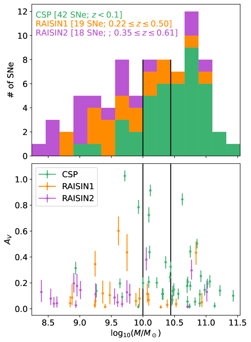
Figure 1: Estimated dust extinction ($A_{V}$) and host galaxy stellar mass ($\log_{10}(M/\mathrm{M}_{\odot})$) for the CSP and RAISIN samples. Vertical lines correspond to host galaxy stellar masses of $10^{10}$ and $10^{10.44}~{}\mathrm{M}_{\odot}$. (top panel) Stacked histogram of $\log_{10}(M/\mathrm{M}_{\odot}$). (bottom panel) Estimated $A_{V}$ vs. $\log_{10}(M/\mathrm{M}_{\odot}$).

Figure 1 shows the $A_{V}$ and host galaxy stellar mass distribution for the CSP, RAISIN1, and RAISIN2 samples. This depicts graphically the mass distributions summarised in the paragraph above, and gives a sense of the number of SNe with moderate-to-high $A_{V}$ in each mass/redshift bin. The SNe with higher $A_{V}$ will have more influence on the $R_{V}$ inference, so the way these are distributed across surveys and host mass will inform us which SNe are driving the results in later sections.

A full description of the photometric data can be found in Jones et al. (2022, §2), with details regarding sample selection in Jones et al. (2022, §3.4). Two example light curves from RAISIN are shown in Figure 2, together with fits made using the BayeSN model.

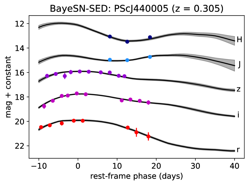
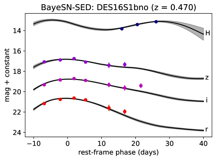
Figure 2: Examples of SN Ia light curve data from the RAISIN1 (upper panel) and RAISIN2 (lower panel) surveys. The RAISIN1 optical ($riz$) data are from the Pan-STARRS Medium Deep Survey, whilst for RAISIN2 these data are from the Dark Energy Survey. The $J$- and $H$-band data are from the Hubble Space Telescope $F125W$ and $F160W$ filters. Also shown are fits to the data using the M20 BayeSN model. The vertical offsets applied for plotting are $(-2,-4,-6,-8,-11)$ for $(r,i,z,J,H)$.

3 Model

We perform our analysis using the BayeSN hierarchical Bayesian model for the spectral energy distributions (SEDs) of SNe Ia (Mandel et al., 2022; Grayling et al., 2024). This framework models variations in the time-dependent SN Ia SED in terms of distinct intrinsic and dust components, as summarised below. We use the M20 version of the model, presented in Mandel et al. (2022), and trained on low-redshift $BVRIYJH$ light curves compiled by Avelino et al. (2019) from the CfA/CfAIR Supernova Programs (Hicken et al., 2009, 2012; Wood-Vasey et al., 2008; Friedman et al., 2015), Carnegie Supernova Project (Krisciunas et al., 2017), and elsewhere in the literature (see references in Avelino et al., 2019; Mandel et al., 2022). This is the same version of the model as was used in the previous analyses by Jones et al. (2022), Thorp & Mandel (2022), and Dhawan et al. (2023). The model covers a rest-frame wavelength range of $\sim 3500$–18500 Å.

We adopt the same hierarchical Bayesian fitting procedure as Thorp & Mandel (2022, §3.2 (ii)), whereby all supernovae in the sample (or a subsample thereof) are fitted simultaneously with the M20 BayeSN model. For each supernova, $s$, we fit for a set of latent parameters, $\bm{\phi}_{s}$. These include the distance modulus, $\mu_{s}$; host galaxy dust extinction, $A_{V}^{s}$; the light curve shape, $\theta_{1}^{s}$; a vector of residual intrinsic SED perturbations, $\bm{e}_{s}$; and a grey (i.e. constant in time and wavelength) luminosity offset, $\delta M_{s}$. Depending on our model configuration, we may also fit for individual values of the total-to-selective extinction ratio, $R_{V}^{s}$, along the line of sight in each supernova’s host galaxy. At the population level, we fit for the population mean dust extinction, $\tau_{A}$, that parameterises an exponential population distribution. We also fit for either a single common $R_{V}$, or, in the case of a $R_{V}^{s}$ population distribution, its mean, $\mu_{R}$, and standard deviation, $\sigma_{R}$. In the latter case, we sample the joint posterior distribution,

$$P(\{\mu_{s},\bm{\phi}_{s}\},\mu_{R},\sigma_{R},\tau_{A}|\{\bm{\hat{f}}_{s},z_{s}\},\bm{\hat{W}}_{0},\bm{\hat{W}}_{1},\bm{\hat{\Sigma}}_{\epsilon},\hat{\sigma}_{0})\\ \propto\bigg{[}\prod_{s}P(\bm{\hat{f}}_{s}|\mu_{s},A_{V}^{s},R_{V}^{s},\theta_{1}^{s},\delta_{M}^{s},\bm{e}_{s},\bm{\hat{W}}_{0},\bm{\hat{W}}_{1})\\ \times P(\mu_{s}|z_{s})\times P(\theta_{1}^{s})\times P(A_{V}^{s}|\tau_{A})\times P(R_{V}^{s}|\mu_{R},\sigma_{R})\\ \times P(\bm{e}_{s}|\bm{\hat{\Sigma}}_{\epsilon})\times P(\delta M_{s}|\hat{\sigma}_{0})\bigg{]}\times P(\tau_{A})\times P(\mu_{R})\times P(\sigma_{R}),$$ (1)

following Thorp & Mandel (2022, eq. 9). Here, $\bm{\hat{W}}_{0}$, $\bm{\hat{W}}_{1}$, $\bm{\hat{\Sigma}}_{\epsilon}$, and $\hat{\sigma}_{0}$ are hyperparameter estimates obtained from model training. Respectively, these are the population mean SED function, a functional principal component capturing the primary mode of SED shape variation, a covariance matrix of intrinsic residual perturbations, and the level of grey residual brightness scatter. The first term inside the product is our flux data likelihood (constructed as per Mandel et al., 2022). The remaining terms in the product are our are our priors on the latent parameters:

$$P(\mu_{s}|\,z_{s}) =N(\mu_{s}|\,\hat{\mu}_{\text{ext},s},\hat{\sigma}_{\text{ext},s}^{2}),$$ (2)

$$P(A_{V}^{s}|\tau_{A}) =\operatorname{Exponential}(A_{V}^{s}|\tau_{A}),$$ (3)

$$P(R_{V}^{s}|\,\mu_{R},\sigma_{R}) =N(R_{V}^{s}|\mu_{R},\sigma_{R}^{2})\text{ for }R_{V}^{s}\geq 0.5,$$ (4)

$$P(\theta_{1}^{s}) =N(\theta_{1}^{s}|\,0,1^{2}),$$ (5)

$$P(\bm{e}_{s}|\bm{\hat{\Sigma}}_{\epsilon}) =N(\bm{e}_{s}|\,\bm{0},\bm{\hat{\Sigma}}_{\epsilon}),$$ (6)

$$P(\delta M_{s}|\,\hat{\sigma}_{0}) =N(\delta M_{s}|0,\hat{\sigma}_{0}^{2}).$$ (7)

Here, we set our distance constraint, $P(\mu_{s}|z_{s})$, based on an external redshift-based distance estimate, $\hat{\mu}_{\text{ext},s}$, and its uncertainty, $\hat{\sigma}_{\text{ext},s}$. Our method for estimating these is given in Section 2. For our hyperpriors, we adopt

$$P(\tau_{A}) =\operatorname{Half-Cauchy}(\tau_{A}|0,1),$$ (8)

$$P(\mu_{R}) =U(\mu_{R}|1,5),$$ (9)

$$P(\sigma_{R}) =\text{Half-}N(\sigma_{R}|0,2^{2}),$$ (10)

following Mandel et al. (2022), Thorp et al. (2021), and Thorp & Mandel (2022).

When fitting for a single common $R_{V}$ within a sample or subsample, we sample the joint posterior distribution given by

$$P(\{\mu_{s},\bm{\phi}_{s}\},R_{V},\tau_{A}|\{\bm{\hat{f}}_{s},z_{s}\},\bm{\hat{W}}_{0},\bm{\hat{W}}_{1},\bm{\hat{\Sigma}}_{\epsilon},\hat{\sigma}_{0})\\ \propto\bigg{[}\prod_{s}P(\bm{\hat{f}}_{s}|\mu_{s},A_{V}^{s},R_{V},\theta_{1}^{s},\delta_{M}^{s},\bm{e}_{s},\bm{\hat{W}}_{0},\bm{\hat{W}}_{1})\times P(\mu_{s}|z_{s}))\times P(\theta_{1}^{s})\\ \times P(A_{V}^{s}|\tau_{A})\times P(\bm{e}_{s}|\bm{\hat{\Sigma}}_{\epsilon})\times P(\delta M_{s}|\hat{\sigma}_{0})\bigg{]}\times P(\tau_{A})\times P(R_{V}).$$ (11)

The priors and hyperpriors here are as given in Equations 2, 3, 5–8, with our hyperprior on the common $R_{V}$ being given by

$$P(R_{V})=U(R_{V}|1,6).$$ (12)

Complete details of the BayeSN model can be found in Mandel et al. (2022), with specific discussion regarding its application to dust being included in Thorp et al. (2021), Thorp & Mandel (2022), and Grayling et al. (2024). As described therein, to fit these statistical models to the data, we use Hamiltonian Monte Carlo (within Stan; Carpenter et al., 2017) to sample the posterior distributions above and use standard diagnostics (Gelman & Rubin, 1992; Betancourt et al., 2014; Betancourt, 2016; Vehtari et al., 2021) to assess the chains.

4 Results

4.1 Common Dust Law Inference

In this Section, we present results from estimating the best fitting common $R_{V}$ value for different subsamples of our data. Whilst assuming a common $R_{V}$ in each subsample is a strong assumption, it allows us to obtain tighter constraints than the more flexible model where an $R_{V}$ population distribution of non-zero width is permitted (Section 4.2 presents our results under this more relaxed assumption). The assumption that SNe in a particular redshift range might be well modelled by a single common $R_{V}$ is an approximation, but it can still provide important information about the typical nature of dust in the subsamples analysed.

With this in mind, we will proceed in Section 4.1.1 to present our inferences of $R_{V}$ in the CSP ($z<0.1$) and RAISIN ($0.22\leq z\leq 0.61$) subsamples of our data. In Section 4.1.2, we will further split these two subsamples by host galaxy stellar mass – testing if there is mass dependence of $R_{V}$ in either redshift bin, and if this may differ as a function of redshift.

4.1.1 Split by Redshift

In the first instance, we perform our inference within three subsamples: CSP ($z<0.1$), RAISIN1 ($0.22\leq z\leq 0.50$), and RAISIN2 ($0.35\leq z\leq 0.61$). Figure 3 shows our posterior distributions of $R_{V}$, and the mean dust extinction, $\tau_{A}$, for these three samples. These results show strong consistency between the posterior distributions for the two RAISIN samples (purple and orange contours in Fig. 3), so we will combine these in subsequent analyses into a single higher-$z$ RAISIN1+2 sample, which will have greater constraining power.

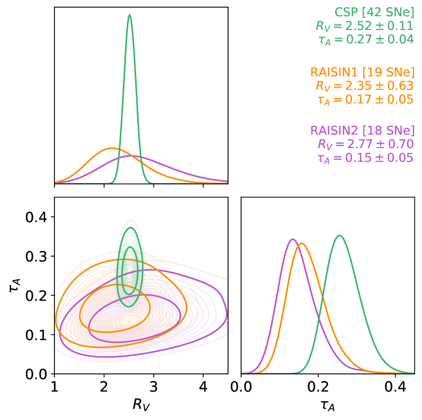
Figure 3: Posterior distributions of the best fitting dust law $R_{V}$, and population mean extinction, $\tau_{A}$, for the three subsamples of our data. Green contours show the CSP sample ($z<0.1$), whilst orange and purple contours show RAISIN1 ($0.22\leq z\leq 0.50$) and RAISIN2 ($0.35\leq z\leq 0.61$), respectively. Parameter summaries are posterior mean $\pm$ standard deviation.

Figure 4 shows our posterior distributions of $R_{V}$ and $\tau_{A}$ for the CSP sample (indicated by the green contours, which are the same as in Fig. 3), and for the combined RAISIN1+2 sample (red contours). For CSP, we estimate $R_{V}=2.52\pm 0.11$, whilst for RAISIN1+2, we estimate $R_{V}=2.37\pm 0.39$, consistent with CSP to within the uncertainties. The estimate we obtain here for CSP is highly consistent with the population mean $R_{V}$ ($\mu_{R}=2.50\pm 0.12$) estimated by Thorp & Mandel (2022) using a slightly larger sample of 75 CSP SNe Ia with apparent $B-V\leq 0.3$. For CSP, we estimate $\tau_{A}=0.27\pm 0.04$ mag, somewhat higher that the estimate of $\tau_{A}=0.15\pm 0.03$ that we obtain for RAISIN1+2. This is unsurprising, as it is likely that the RAISIN sample will be biased towards low-$A_{V}$ SNe due to the difficulty of detecting these objects at high redshift (see also the discussion of similar results in the optical analysis of Grayling et al., 2024). We defer a Bayesian treatment of this selection effect to future work.

Figure 4: Same as Figure 3, but showing results where the two RAISIN subsamples were merged and assumed to have a common $R_{V}$ and extinction distribution. Red contours show the inference for this combined RAISIN1+2 sample. Green contours show CSP, as in Figure 3.

From the posterior samples shown in Figure 4, we can derive a posterior distribution of the high- vs. low-$z$ (i.e. RAISIN vs. CSP) $R_{V}$ difference ($\Delta R_{V}^{z}=R_{V}^{\text{RAISIN}}-R_{V}^{\text{CSP}}$). Figure 5 shows this. From this, we can estimate that $-0.84<\Delta R_{V}^{z}<0.71$, with 95 per cent posterior probability. This is fully consistent with a picture in which there is no evolution in the typical $R_{V}$ as a function of redshift, but does not rule out a shift in either direction.

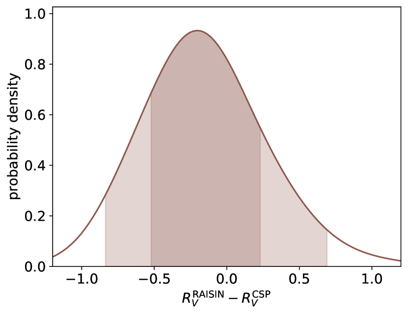
Figure 5: Posterior probability distribution of the $R_{V}$ difference between the high-$z$ RAISIN sample, and low-$z$ CSP sample. Shaded regions show 68 and 95 per cent credible intervals.

4.1.2 Split by Redshift and Host Galaxy Mass

In this section, we perform our inference with the CSP and RAISIN samples each being split by host galaxy stellar mass, giving four subsamples in total. We follow Jones et al. (2022) in choosing the sample split points to test, considering splits at $10^{10}~{}\mathrm{M}_{\odot}$, and at $10^{10.44}~{}\mathrm{M}_{\odot}$. The latter corresponds to a best-fitting NIR mass step location identified by Ponder et al. (2021) using the Akaike Information Criterion.

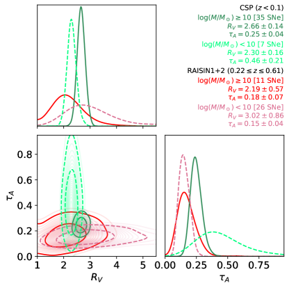
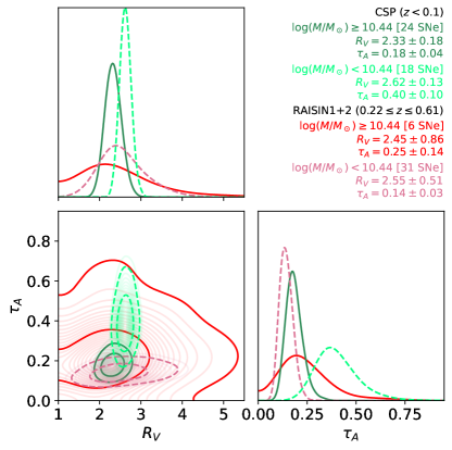
Figure 6: Same as Figure 4, but with the low-redshift CSP sample ($z<0.1$) and higher-redshift RAISIN sample ($0.22\leq z\leq 0.61$) each subdivided by host galaxy stellar mass. Green contours show CSP, whilst red/pink contours show RAISIN. Darker solid contours show higher host galaxy masses, whilst lighter dashed contours show lower host masses. We use the two sample split points used by Jones et al. (2022) as their default choice and systematic test. (left panels) Inference when the sample is split at the default host galaxy stellar mass of $10^{10}~{}\mathrm{M}_{\odot}$. (right panels) Split at $10^{10.44}~{}\mathrm{M}_{\odot}$, the best fitting NIR mass step location found by Ponder et al. (2021).

Figure 6 shows our posterior distributions for $R_{V}$ and $\tau_{A}$ in the low- and high-host mass RAISIN and CSP samples. The left hand panels show the results for the $10^{10}~{}\mathrm{M}_{\odot}$ mass split, with the right showing the split at $10^{10.44}~{}\mathrm{M}_{\odot}$. In terms of $R_{V}$, the picture is generally one of consistency to within the uncertainties. For CSP, we estimate $R_{V}=2.30\pm 0.16$ for host galaxies less massive than $10^{10}~{}\mathrm{M}_{\odot}$, and $2.66\pm 0.14$ for more massive hosts. In the higher-redshift bin, the estimates of $R_{V}$ are more uncertain. Within these uncertainties, the $R_{V}$ estimates for the two mass bins are consistent with one another, and with their low-redshift counterparts.

Following on from Fig. 5 in Section 4.1.1, we can use our posterior samples to derive probability distributions of the change in $R_{V}$ with either redshift (in the two mass bins), or mass (in the two redshift bins). This allows us to investigate two related questions:

1. Is the potential evolution of $R_{V}$ with redshift ($\Delta R_{V}^{z}=R_{V}^{\text{RAISIN}}-R_{V}^{\text{CSP}}$) different for low- and high-mass host galaxies?

2. Are the potential correlations of $R_{V}$ with mass ($\Delta R_{V}^{M}=R_{V}^{\text{high-}M}-R_{V}^{\text{low-}M}$) different at low- and high-redshift?

We will tackle the first question first, and will estimate the posterior probability distributions of $\Delta R_{V}^{z}=R_{V}^{\text{RAISIN}}-R_{V}^{\text{CSP}}$ separately for high- and low-mass host galaxies. Figure 7 shows the resulting posteriors for the $10^{10}~{}\mathrm{M}_{\odot}$ and $10^{10.44}~{}\mathrm{M}_{\odot}$ mass splits. For both mass splits, the picture is fairly uncertain, but there is not significant evidence that the high- vs. low-$z$ $\Delta R_{V}^{z}$ differs for low- and high-mass hosts. For the split at $10^{10}~{}\mathrm{M}_{\odot}$, the $\Delta R_{V}^{z}$ distribution for high-mass hosts leans towards negative values (i.e. lower $R_{V}$ at higher $z$), whereas the $\Delta R_{V}^{z}$ distribution for low-mass hosts leans towards positive values (i.e. higher $R_{V}$ at higher $z$). Zero is within the 68 per cent credible interval for both mass bins, however, and both bins have significant posterior density at both positive and negative values of $\Delta R_{V}^{z}$. For the split at $10^{10.44}~{}\mathrm{M}_{\odot}$ (left panel of Fig. 7), the picture is similar, although the $\Delta R_{V}^{z}$ posteriors in the two mass bins are more similar in this case, both having their modes very close to $\Delta R_{V}^{z}=0$, and having slightly longer tails towards positive $\Delta R_{V}^{z}$.

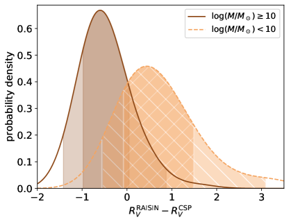
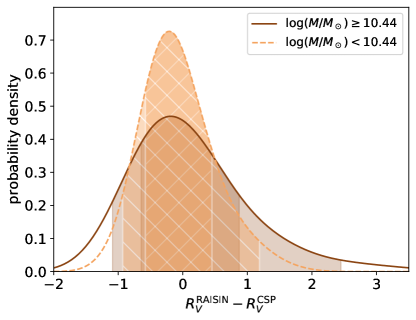
Figure 7: Same as Figure 5, but with the sample split into two bins of high (solid dark brown curves) and low (dashed light brown curves) host galaxy mass. (left panel) Sample divided at $10^{10}~{}\mathrm{M}_{\odot}$. (right panel) Sample divided at $10^{10.44}~{}\mathrm{M}_{\odot}$.

To tackle the second question, we will estimate the posterior distributions of $\Delta R_{V}^{M}=R_{V}^{\text{high-}M}-R_{V}^{\text{low-}M}$ separately for the RAISIN (high-$z$) and CSP (low-$z$) samples. Figure 8 shows this for the $10^{10}~{}\mathrm{M}_{\odot}$ and $10^{10.44}~{}\mathrm{M}_{\odot}$ mass splits. For both mass splits, the resulting posterior distribution is much tighter for the CSP sample than RAISIN. The results are consistent for the two mass splits, and do not provide statistically significant evidence for a changing $\Delta R_{V}^{M}$ between low- and high-redshift. For the CSP sample, the $\Delta R_{V}^{M}$ posterior has more probability towards positive values (i.e. higher $R_{V}$ in higher mass galaxies) for the $10^{10}~{}\mathrm{M}_{\odot}$ mass split, but more towards negative values for the $10^{10.44}~{}\mathrm{M}_{\odot}$ mass split. The latter is more in line with our previous results at low-$z$ (see Thorp et al., 2021; Thorp & Mandel, 2022), although both there and here the estimated $\Delta R_{V}^{M}$ (or $\Delta\mu_{R}^{M}$ in Thorp & Mandel, 2022) has not been significantly different from zero. Indeed, for both mass splits considered here, $\Delta R_{V}^{M}=0$ is within the 95 per cent posterior credible intervals for CSP. For RAISIN, the posteriors show a mild tendency towards negative $\Delta R_{V}^{M}$ (i.e. lower $R_{V}$ for higher mass host galaxies) for both choices of mass split, although $\Delta R_{V}^{M}=0$ is within the 68 per cent credible interval in both cases. The results for the $10^{10}~{}\mathrm{M}_{\odot}$ mass split would be consistent with a larger potential redshift evolution of $\Delta R_{V}^{M}$ than the results for $10^{10.44}~{}\mathrm{M}_{\odot}$, although due to the large uncertainties in both cases, there is no statistically significant evidence for such a redshift evolution in either case.

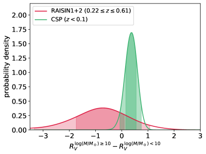
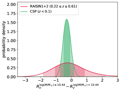
Figure 8: Same as Figure 7, but showing high- vs. low-mass $\Delta R_{V}^{M}$ for the two redshift bins (rather than high- vs. low-$z$ $\Delta R_{V}^{z}$ for the two mass bins). (left panel) Sample divided at $10^{10}~{}\mathrm{M}_{\odot}$. (right panel) Sample divided at $10^{10.44}~{}\mathrm{M}_{\odot}$.

4.2 Dust Law Population Distribution Inference

In this Section, we relax the assumption that each SN Ia subsample is consistent with a single $R_{V}$ common to that subsample. Instead, we assume a Gaussian population distribution of $R_{V}$, with the $R_{V}^{s}$ for a supernova, $s$, being modelled as a draw from this population distribution, like so: $R_{V}^{s}\sim N(\mu_{R},\sigma_{R}^{2})$. When we perform our inference, we sample from the joint posterior distribution given by Equation 1, conditional on the data for a given supernova subsample. We marginalize over all supernova-level parameters, including the set of individual $R_{V}^{s}$ values, to obtain a posterior distribution over the $R_{V}$ population mean, $\mu_{R}$, and standard deviation, $\sigma_{R}$.

In Section 4.2.1, we present our results for the low-$z$ CSP data, and higher-$z$ RAISIN data. In Section 4.2.2, we present results obtained by combining the CSP and RAISIN samples, and then splitting this combined sample by host galaxy stellar mass.

4.2.1 Split by Redshift

As in Section 4.1.1, we will begin by performing an analysis with the sample split by redshift. Figure 9 shows our posterior distributions of the $R_{V}$ population mean ($\mu_{R}$) and standard deviation ($\sigma_{R}$), and $A_{V}$ population mean ($\tau_{A}$). Our estimates of $\tau_{A}$ for the two samples are identical to those obtained from the analysis in the previous sections (see Fig. 4 and Section 4.1.1). We have previously found that inference of the mean dust extinction, $\tau_{A}$, is very insensitive to the assumption of a single $R_{V}$ or population distribution thereof, so this result is unsurprising (see Thorp et al., 2021).

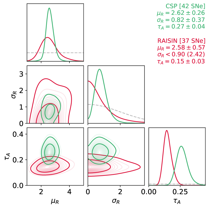
Figure 9: Posterior distributions of the host galaxy dust population distribution parameters for the CSP ($z<0.1$; green contours) and RAISIN ($0.2\lesssim z\lesssim 0.6$; red countours) components of our sample. Parameters plotted are the mean ($\mu_{R}$) and standard deviation ($\sigma_{R}$) of the Gaussian $R_{V}$ population distribution, and the mean ($\tau_{A}$) of the exponential $A_{V}$ distribution. Parameter summaries are ether posterior mean $\pm$ standard deviation, or 68 (95)th posterior percentile. Dashed lines indicate the hyperpriors.

For CSP, we estimate an $R_{V}$ population mean of $\mu_{R}=2.62\pm 0.26$, and a population standard deviation of $\sigma_{R}=0.82\pm 0.37$. This population mean estimate is consistent with the common $R_{V}=2.52\pm 0.11$ estimated in Section 4.1.1. Additionally, these population mean and standard deviation estimates are consistent with the estimates obtained by Thorp & Mandel (2022) using a larger sample of 75 CSP SNe Ia with apparent $B-V\leq 0.3$. For RAISIN, we estimate $\mu_{R}=2.58\pm 0.57$, fully consistent with the CSP population mean estimate. Our posterior distribution for $\sigma_{R}$ peaks at zero, meaning we can use the posterior credible intervals to place upper limits on $\sigma_{R}$ in the RAISIN redshift range. We estimate that $\sigma_{R}<0.90$ with 68 per cent posterior probability, and $\sigma_{R}<2.42$ with 95 per cent posterior probability.

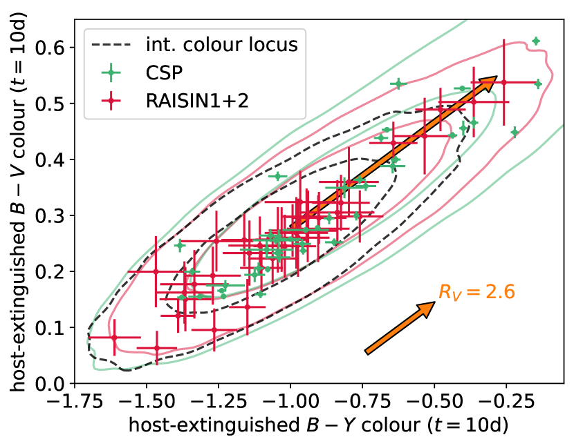
Figure 10: Estimated host-extinguished apparent $B-V$ vs. $B-Y$ colours for RAISIN (red points) and CSP (green points) at a rest-frame phase of 10 d. The red contours show the posterior predictive distribution (PPD) for RAISIN’s host-extinguished colours, with the green showing the PPD for CSP’s colours, from our dust law population inference (§4.2.1, Fig. 9). The black dashed contours show the intrinsic colour locus predicted by the M20 BayeSN model. The contours shown are 68 and 95 per cent credible intervals. The orange arrows show a reddening vector corresponding to $R_{V}=2.6$ (approximately the posterior mean of $\mu_{R}$ for CSP and RAISIN; c.f. Fig. 9). The longer arrow is has its base at the mean of the intrinsic colour locus and has a length corresponding to $A_{V}=0.75$. The shorter arrow has a length corresponding to $A_{V}=0.25$.

Figure 10 shows the estimated host-extinguished apparent $B-V$ and $B-Y$ colours for the RAISIN and CSP samples at a rest frame phase of 10 d. We chose this phase as a trade-off between being close to the data (the median phase of first observation for RAISIN is $\lesssim 9.5$ d; Jones et al., 2022), but also being at a phase where intrinsic colour variation is relatively moderate (both due to correlation with light curve shape, and residual scatter on top of this; c.f. Mandel et al., 2022 fig. 8 & 9). The contours in our Figure 10 show the posterior predictive distributions (PPD) for host-extinguished colours for the two redshift ranges, i.e.

$$P[(B-V)_{t=10\,\mathrm{d}}^{\text{ext}},(B-Y)_{t=10\,\mathrm{d}}^{\text{ext}}|\{\bm{\hat{f}}_{s}\},\bm{\hat{W}}_{0},\bm{\hat{W}}_{1},\bm{\hat{\Sigma}}_{\epsilon}]\\ =\int P(\{\mu_{s},\bm{\phi}_{s}\},\mu_{R},\sigma_{R},\tau_{A}|\{\bm{\hat{f}}_{s}\},\bm{\hat{W}}_{0},\bm{\hat{W}}_{1},\bm{\hat{\Sigma}}_{\epsilon},\hat{\sigma}_{0})\\ \times P[(B-V)_{t=10\,\mathrm{d}}^{\text{ext}},(B-Y)_{t=10\,\mathrm{d}}^{\text{ext}}|\bm{\phi}]\times P(\bm{\phi}|\mu_{R},\sigma_{R},\tau_{A},\bm{\hat{\Sigma}}_{\epsilon})\\ \times d\mu_{s}\,d\bm{\phi}_{s}\,d\mu_{R}\,d\sigma_{R}\,d\tau_{A},$$ (13)

where

$$P(\bm{\phi}|\mu_{R},\sigma_{R},\tau_{A},\bm{\hat{\Sigma}}_{\epsilon})=P(R_{V}|\mu_{R},\sigma_{R})P(A_{V}|\tau_{A})P(\theta_{1})P(\bm{e}|\bm{\hat{\Sigma}}_{\epsilon}).$$ (14)

The PPDs are estimated by simulating supernovae from $P(\bm{\phi}|\mu_{R},\sigma_{R},\tau_{A},\bm{\hat{\Sigma}}_{\epsilon})$, conditional on the $\mu_{R}$, $\sigma_{R}$, and $\tau_{A}$ for each MCMC sample from the posteriors shown in Fig. 9, and computing their $B-V$ and $B-Y$ colours. Also shown in Fig. 10 is the intrinsic colour locus of the M20 BayeSN model, determined by taking draws from the prior $P(\theta_{1})\times P(\bm{e}|\bm{\hat{\Sigma}}_{\epsilon})$ and estimating colours with $A_{V}=0$. The PPD corresponding to the low-$z$ CSP sample is more dispersed along the diagonal than for the higher-$z$ RAISIN sample, reflective of the posterior for CSP in Fig. 9 being weighted towards a higher mean dust extinction, $\tau_{A}$. Although the constraints on the population standard deviation, $\sigma_{R}$, of $R_{V}$ for RAISIN are more uncertain than for CSP, the posterior for CSP is more concentrated towards non-zero values, with a posterior mean of 0.82. In the PPD, this is reflected as a broader distribution of colours perpendicular to the diagonal – particularly towards redder end.

Similarly to in Figure 5, we can compute a derived posterior on the difference in $\mu_{R}$ ($\Delta\mu_{R}^{z}=\mu_{R}^{\text{RAISIN}}-\mu_{R}^{\text{CSP}}$) between the low-$z$ CSP and high-$z$ RAISIN samples. Figure 11 shows this. This posterior distribution is reasonably symmetric, so does not suggest a preference for either of the possible directions of $\mu_{R}$ shift. We can place limits on the possible redshift drift of $\mu_{R}$, estimating that $-0.63<\Delta\mu_{R}^{z}<0.55$ with 68 per cent posterior probability, and $-1.16<\Delta\mu_{R}^{z}<1.38$ with 95 per cent posterior probability.

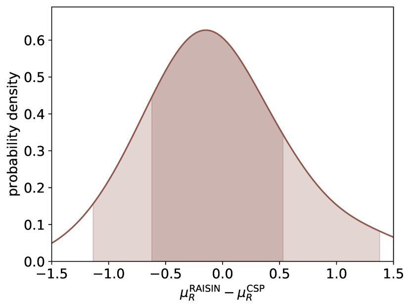
Figure 11: Posterior probability distribution of the estimated high- vs. low-$z$ difference in population mean $R_{V}$ ($\Delta\mu_{R}^{z}$).

4.2.2 Split by Host Galaxy Mass

Motivated by the consistency between the CSP and RAISIN samples seen in Section 4.2.1, in this section we combine the data from the two surveys, and then perform our inference with this joint sample split by host galaxy mass. When fitting the $R_{V}$ population distribution model (Eq. 1), we lack the leverage to split the sample four ways, as we did in Section 4.1.2. Nevertheless, we can still utilise this combined sample to investigate the possible dependence of the $R_{V}$ population distribution on host galaxy stellar mass.

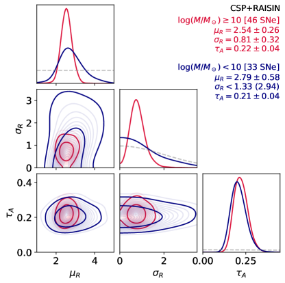
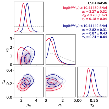
Figure 12: Posterior distributions of the host galaxy dust population distribution parameters of the combined CSP+RAISIN sample, split by host galaxy stellar mass. Red contours show the higher mass subsample, whilst blue show the lower mass subsample. Parameters plotted are the same as in Fig. 9. Mass splits in the left- and right-hand corner plots are the same as in Figure 6.

Figure 12 shows our posterior inference of $\mu_{R}$, $\sigma_{R}$, and $\tau_{A}$ for the mass split CSP+RAISIN sample. We test the same pair of split points ($10^{10}~{}\mathrm{M}_{\odot}$ and $10^{10.44}~{}\mathrm{M}_{\odot}$) as in Section 4.1.2 and Jones et al. (2022). For both choices of split, we estimate consistent $R_{V}$ population distributions in the two mass bins. For host galaxies more massive than $10^{10}~{}\mathrm{M}_{\odot}$, we estimate an $R_{V}$ population distribution with mean $\mu_{R}=2.54\pm 0.26$, and standard deviation $\sigma_{R}=0.81\pm 0.32$. For hosts less massive than $10^{10}~{}\mathrm{M}_{\odot}$, we estimate $\mu_{R}=2.79\pm 0.58$, and place upper limits on $\sigma_{R}<1.33~{}(2.94)$ with 68 (95) per cent posterior probability. For the split at $10^{10.44}~{}\mathrm{M}_{\odot}$, we estimate $\mu_{R}=2.27\pm 0.32$ for high mass hosts, and $\mu_{R}=2.82\pm 0.31$ for low mass hosts. In higher mass hosts, we place an upper limit on $\sigma_{R}<0.78~{}(1.62)$ at the 68 (95) per cent level. In the lower mass hosts, we estimate $\sigma_{R}=0.87\pm 0.43$, albeit with significant posterior probability density near zero (see Fig. 12).

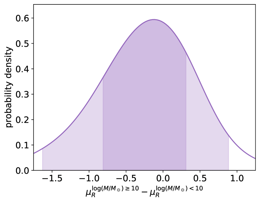
Figure 13: Posterior of low- vs. high-mass $\Delta\mu_{R}^{M}$, for the CSP+RAISIN combined sample split at $10^{10}~{}\mathrm{M}_{\odot}$.

As an alternative to Figure 11, we can use the results from this Section to estimate the posterior distribution of a high- vs. low-mass change in $\mu_{R}$ ($\Delta\mu_{R}^{M}=\mu_{R}^{\text{high-}M}-\mu_{R}^{\text{low-}M}$). Figure 13 shows this for a mass split at $10^{10}~{}\mathrm{M}_{\odot}$. We can see that this shows a slight tendency towards a negative $\Delta\mu_{R}^{M}$ (i.e. a weak preference of higher $\mu_{R}$ in lower-mass host galaxies). However, a $\Delta\mu_{R}^{M}$ of zero (i.e. no difference) is well within the 68 per cent credible interval. With 68 per cent posterior probability, we estimate that $-0.83<\Delta\mu_{R}^{M}<0.34$, and with 95 per cent posterior probability, we estimate $-1.66<\Delta\mu_{R}^{M}<0.91$. We do not include a Figure for the $10^{10.44}~{}\mathrm{M}_{\odot}$ split, but the picture is very similar, albeit with a slightly stronger tendency towards negative $\Delta\mu_{R}^{M}$. For this split, we estimate $-0.97<\Delta\mu_{R}^{M}<-0.12$ at the 68 per cent level, and $-1.46<\Delta\mu_{R}^{M}<0.35$ at the 95 per cent level.

5 Conclusions

In this paper, we have used our BayeSN hierarchical model to analyse high-$z$ SN Ia light curves from the RAISIN Survey (Jones et al., 2022), along with a complementary set of low-$z$ SNe Ia from CSP. We have presented constraints on the dust law $R_{V}$ (and its population distribution) in SN Ia host galaxies for this redshift range ($0.22\leq z\leq 0.61$). This is the first such analysis using RAISIN data, and our results are the first SN Ia host galaxy $R_{V}$ constraints at high-$z$ to be based on rest-frame optical and NIR data.

Assuming a single common dust law can describe the RAISIN sample, we estimate $R_{V}=2.37\pm 0.39$. This is fully consistent with the value of $R_{V}=2.52\pm 0.11$ that we estimate for the low-$z$ CSP sample (which, in turn, is fully consistent with our low-$z$ $R_{V}$ estimates from previous analyses; Thorp et al., 2021; Thorp & Mandel, 2022; Ward et al., 2023a; Grayling et al., 2024). We use these results to place probabilistic limits on the shift in $R_{V}$ between low- and high-redshift ($\Delta R_{V}^{z}=R_{V}^{\text{RAISIN}}-R_{V}^{\text{CSP}}$), estimating that $-0.84<\Delta R_{V}^{z}<0.71$, with 95 per cent posterior probability. This constraint does not rely on assuming that $R_{V}$ is associated with a particular galaxy type/property, and propagating that indirectly to a constraint on $\Delta R_{V}^{z}$ based on a model for galaxy evolution across cosmic time. Rather, it a direct constraint of $\Delta R_{V}^{z}$, conditional on the data. This has the advantage of depending on fewer astrophysical assumptions, and does not assume that an estimated low-$z$ correlation between $R_{V}$ and host properties perseveres at high-$z$. However, a direct $\Delta R_{V}^{z}$ constraint cannot be easily projected beyond the redshift range of the data that it is obtained from (c.f. the progenitor-based mass step model of Rigault et al., 2013 or Childress et al., 2014; or the linear $\mu_{R}$ vs. redshift relation of Grayling et al., 2024). Additionally, the utility of a direct constraint requires the high- and low-$z$ samples analysed to be representative (in terms of dust properties, at least) of the broader population of SN Ia hosts in their respective redshift ranges. With CSP-I leaning heavily towards the follow-up of SNe from “targeted” searches (see Krisciunas et al., 2017 §2, and references therein), the low-$z$ component of our sample will not have a host galaxy distribution that is representative of low-$z$ SN hosts more generally. However, our previous work has yielded consistent inferences about $R_{V}$ when using the CSP data (Thorp & Mandel, 2022), and when using a more “untargeted” low-$z$ sample (Thorp et al., 2021; using data from the Foundation Supernova Survey; Foley et al., 2018b; Jones et al., 2019), suggesting that this may not be a major cause for concern.

Due to the caveats associated with our estimated limits on $\Delta R_{V}^{z}$, we will forgo a detailed propagation of these limits into an estimate of potential cosmological bias. Such an effort will be better deferred to a future study incorporating a treatment of selection effects. This could be achieved via a survey-simulation-based approach using SNANA (Kessler et al., 2009a) as in the RAISIN cosmology analysis (Jones et al., 2022), by integrating a Bayesian selection effect treatment (à la UNITY; Rubin et al., 2015, 2023; or BAHAMAS; Shariff et al., 2016; Rahman et al., 2022) into our own hierarchical model, or via simulation based inference (e.g. Karchev et al., 2023b). Independent of any implications for cosmology, however, constraints on dust from SNe Ia can still provide a unique insight into dust in galaxies beyond the Milky Way, complementary to the information provided by different probes. As pointed out by Keel et al. (2023), SNe Ia (being distributed fairly uniformly throughout their hosts; e.g. Galbany et al., 2014) can give valuable information about the dust further from bright or star forming regions, and they provide information about the dust extinction along specific sightlines (rather than the integrated effect of dust over a large region or the whole galaxy).

As well as estimating the single best-fitting $R_{V}$ values in the low- and high-$z$ samples, we also perform an analysis where the assumption of zero variance is relaxed, and the parameters (mean, $\mu_{R}$, and standard deviation, $\sigma_{R}$) of a Gaussian $R_{V}$ population distribution are fitted. For the low-$z$ CSP sample we estimate $\mu_{R}=2.62\pm 0.26$ and $\sigma_{R}=0.82\pm 0.37$, whilst for the high-$z$ RAISIN sample we estimate $\mu_{R}=2.58\pm 0.57$ and place an upper limit on $\sigma_{R}<0.90~{}(2.42)$ with 68 (95) per cent posterior probability. Our population distribution estimate at low-$z$ is consistent with our previous analyses (Thorp et al., 2021; Thorp & Mandel, 2022), and the estimates at high- and low-$z$ are consistent to within their uncertainties. As with the single-$R_{V}$ analysis, we are able to place limits on the potential redshift drift of the mean $R_{V}$ ($\Delta\mu_{R}^{z}=\mu_{R}^{\text{RAISIN}}-\mu_{R}^{\text{CSP}}$), finding that $-1.16<\Delta\mu_{R}^{z}<1.38$ with 95 per cent posterior probability. The credible interval here is slightly wider than the equivalent $\Delta R_{V}^{z}$ posterior, and permits a wide range of possibilities. Analysis of a large optical sample (Grayling et al., 2024) has yielded similar constraints. Nevertheless, it allows us to confidently rule out very extreme drifts in mean $R_{V}$ of $\gtrsim 1.5$, and is a promising preliminary result that should be built on in future analyses.

Finally, given the consistency of our $R_{V}$ population distribution inferences in the CSP and RAISIN samples, we use the combined CSP+RAISIN data to investigate the mass-dependence of the host galaxy $R_{V}$ distribution. In combination, these data have a fairly even split between host masses above and below $10^{10}~{}\mathrm{M}_{\odot}$ ($46/79$ above, $33/79$ below), albeit with the quirk that the high-mass subset is dominated by CSP ($35/46$), whilst the low-mass subset is dominated by RAISIN ($26/33$). For host galaxies more massive than $10^{10}~{}\mathrm{M}_{\odot}$, we estimate an $R_{V}$ population distribution with mean $\mu_{R}=2.54\pm 0.26$, and standard deviation $\sigma_{R}=0.81\pm 0.32$. For hosts less massive than $10^{10}~{}\mathrm{M}_{\odot}$, we estimate $\mu_{R}=2.79\pm 0.58$, and $\sigma_{R}<1.33~{}(2.94)$ at the 68 (95) per cent level. Our results can be propagated to a constraint on the high- minus low-mass difference in $\mu_{R}$ ($\Delta\mu_{R}^{M}=\mu_{R}^{\text{high-}M}-\mu_{R}^{\text{low-}M}$), leading to a 95 per cent credible interval encompassing $-1.66<\Delta\mu_{R}^{M}<0.91$. For an alternative sample split at $10^{10.44}~{}\mathrm{M}_{\odot}$, the results are similar – i.e. no strong exclusion of $\Delta\mu_{R}^{M}=0$.

In summary, we have utilised the unique high-$z$ rest-frame NIR data provided by the RAISIN Survey to investigate the mass- and redshift-dependence of the dust law $R_{V}$ in SN Ia host galaxies. Regarding the potential redshift-evolution of $R_{V}$ (independent of other host galaxy properties), we have placed direct constraints on the difference in (mean) $R_{V}$ between SN Ia hosts at $z<0.1$ and $0.2\lesssim z\lesssim 0.6$. These are the first constraints of this nature to make use of rest-frame NIR data across the full redshift range studied. We do not find statistically significant evidence for a non-zero shift in mean $R_{V}$ between low- and high-$z$, and are able to rule out an absolute shift in mean $R_{V}$ of $\gtrsim 1.5$ with high confidence. These results complement the optical analysis of Grayling et al. (2024), who estimate a $\mu_{R}$ vs. $z$ correlation coefficient of $\eta_{R}=-0.38\pm 0.70$. Given that a shift in $R_{V}$ or the colour–luminosity coefficient $\beta$ by $\approx 1.4$ between low- and high-$z$ could easily propagate to a significant bias in $w$, future work is needed to control this potential systematic.

The analysis we have presented here lays the groundwork for future NIR investigations, and can be developed further via the incorporation of a robust Bayesian treatment of selection effects (see e.g. Rubin et al., 2015; Shariff et al., 2016; Rahman et al., 2022; Karchev et al., 2023b; Rubin et al., 2023). Investigation of intrinsic colour evolution with redshift would also be a worthwhile avenue to pursue. The promising results we have obtained using a sample of 37 high-$z$ SNe Ia illustrate the value of having rest-frame NIR data at higher redshifts, adding to the case already made by the RAISIN cosmology results (Jones et al., 2022). Such data could potentially be obtained by the Roman Space Telescope HLTDS (Hounsell et al., 2018; Rose et al., 2021a), although the current reference survey design prioritises the rest-frame optical (Rose et al., 2021a). A design more focused on the rest frame NIR could be hugely valuable, and would be a great complement to the rest-frame optical data obtained by LSST (for further discussion of Roman–LSST synergies, see Foley et al., 2018a; Rhodes et al., 2019; Rose et al., 2021b; Bianco et al., 2024). The discovery and analysis of SN Ia siblings (multiple SNe Ia in the same host; e.g. Elias et al., 1981; Hamuy et al., 1991; Stritzinger et al., 2010; Gall et al., 2018; Burns et al., 2020; Scolnic et al., 2020; Graham et al., 2022; Kelsey, 2024; Dwomoh et al., 2023) at high-$z$ will also prove complimentary, with these systems offering greater leverage for constraining dust properties and colour–luminosity correlations than galaxies that host a lone optically observed supernova (Biswas et al., 2022; Ward et al., 2023b). In fact, Ward et al. (2023b) liken the leverage gained from the presence of a sibling SN Ia to the benefit gained from having NIR data. Understanding any redshift-dependent systematics/biases associated with host galaxy dust will be of critical importance to the LSST and Roman dark energy analyses. And the impact of these effects is already being felt in current analyses (Vincenzi et al., 2024; DES Collaboration et al., 2024). The continued work by the community to observe (e.g. Wood-Vasey et al., 2008; Friedman et al., 2015; Krisciunas et al., 2017; Phillips et al., 2019; Johansson et al., 2021; Konchady et al., 2022; Müller-Bravo et al., 2022; Jones et al., 2022; Peterson et al., 2023) and model (e.g. Mandel et al., 2009; Mandel et al., 2011; Burns et al., 2011, 2014; Pierel et al., 2018; Avelino et al., 2019; Mandel et al., 2022; Pierel et al., 2022; Grayling et al., 2024) SNe Ia in the NIR will be crucial to furthering our understanding and controlling dust-related systematics.

Data Availability

All data used are publicly available. The Carnegie Supernova Project data are presented in Krisciunas et al. (2017). The data from the RAISIN Survey are presented in Jones et al. (2022). The RAISIN data release containing all relevant light curves is available publicly on GitHub. A new BayeSN code (Grayling et al., 2024) is also available on GitHub and will be integrated into SNANA (Kessler et al., 2009a).

Appendix A SN Ia Dust Laws Since 2020

Over the past three years (beginning roughly with Brout & Scolnic, 2020), there has been a proliferation of analyses that have said something about the $R_{V}$ distribution in SN Ia host galaxies. In Table 1, we attempt to summarise as many key results as possible from this time period. We confine this comparison primarily to studies of samples (as opposed to single SNe), and do not quote every result from each paper in cases where there are many analysis variants. For each study, we state (where applicable) reported values for the following quantities: $R_{V}$ or $\mu(R_{V})$ for the full sample; $\sigma(R_{V})$ for the full sample; $\mu(R_{V})$ and $\sigma(R_{V})$ either side of the “classic” $10^{10}~{}\mathrm{M}_{\odot}$ mass step. By limiting ourselves to the previous three years, we necessarily many omit landmark results in the history of SN Ia host galaxy $R_{V}$ estimation (e.g. Jöeveer, 1982; Riess et al., 1996; Krisciunas et al., 2000, 2007; Folatelli et al., 2010; Mandel et al., 2011; Burns et al., 2014; Mandel et al., 2017). We also note that many of the listed papers presented more analysis variants than we can easily summarise here.

Table 1: Literature $R_{V}$ estimates for populations of SN Ia hosts since 2020.

Paper	Modela	Data Typeb	Sample	$R_{V}$c	$\mu(R_{V})$d	$\sigma(R_{V})$e	$\mu(R_{V})|$HMf	$\sigma(R_{V})|$HMf	$\mu(R_{V})|$LMg	$\sigma(R_{V})|$LMg
Léget et al. (2020)	SUGAR	Spec.	SNfactory1	2.60	-	-	-	-	-	-
Brout & Scolnic (2021)å	SALT2${\dagger}$	Phot.	Various2–8	-	$2.00\pm 0.20$	$1.40\pm 0.20$	$1.50\pm 0.25$	$1.30\pm 0.20$	$2.75\pm 0.35$	$1.30\pm 0.20$
Thorp et al. (2021)	BayeSN	Phot.	Foundation4	$2.61\pm 0.21$	$2.70\pm 0.25$	0.37 (0.61)	$2.72\pm 0.23$	0.32 (0.62)	$3.49\pm 0.61$	0.89 (1.87)
Johansson et al. (2021)	SNooPy§	Phot.	Various NIR2,3,9–12	-	1.90	$0.90$	1.70	0.80	2.20	0.90
Arima et al. (2021)	Multiband Stretch*	Phot.	Low-$z$13	$3.00^{+0.40}_{-0.30}$	-	-	-	-	-	-
Mandel et al. (2022)	BayeSN	Phot.	Low-$z$ NIR14	$2.89\pm 0.20$	-	-	-	-	-	-
Thorp & Mandel (2022)	BayeSN	Phot.	CSP3	-	$2.59\pm 0.14$	$0.62\pm 0.16$	$2.54\pm 0.15$	$0.56\pm 0.18$	$2.78\pm 0.70$	1.62 (3.01)
Wiseman et al. (2022)å	SALT2	Phot.	DES5YR15	-	-	-	1.75	1.00	3.00	1.00
Popovic et al. (2023)ä	SALT2	Phot.	Pantheon+16	-	-	-	$2.14\pm 0.25$	$1.06\pm 0.43$	$3.03\pm 0.38$	$1.48\pm 0.42$
Ward et al. (2023a)	GP$\infty$	Phot.	Low-$z$ NIR2,3,9,10	-	$2.61^{+0.38}_{-0.35}$	0.92 (1.96)	-	-	-	-
Meldorf et al. (2023)ö	Bagpipes||	Gal. Phot.	DES5YR15,17	-	-	-	$2.61\pm 0.07$	$0.86\pm 0.06$	$3.02\pm 0.05$	$0.82\pm 0.04$
Duarte et al. (2023)	Prospector¶	Gal. Phot.	DES3YR5,18	-	-	-	$2.67\pm 0.11$	0.97	$3.09\pm 0.13$	1.16
Smadja et al. (2023)	Other$\nabla$	Spec., Phot.	SNfactory1	$2.22\pm 0.17$	-	-	-	-	-	-
Wojtak et al. (2023)	SALT2	Phot.	SuperCal19	-	$3.13^{+0.65}_{-0.59}$	$0.95^{+0.31}_{-0.28}$	-	-	-	-
Karchev et al. (2023a)æ	BayeSN	Phot.	CSP3	-	-	-	-	-	-	-
Vincenzi et al. (2024)ä	SALT3${\ddagger}$	Phot.	DES5YR15	-	-	-	1.66	0.95	3.25	0.93
Grayling et al. (2024)	BayeSN	Phot.	Various4–6	-	$2.58\pm 0.14$	$0.59\pm 0.20$	$2.51\pm 0.16$	$0.47\pm 0.21$	$2.74\pm 0.35$	$0.93\pm 0.32$
Grayling et al. (2024)ø	BayeSN	Phot.	Various4–6	-	-	-	$2.26\pm 0.14$	0.27 (0.49)	$3.36\pm 0.51$	1.07 (1.81)
Thorp et al. (this work)	BayeSN	Phot.	CSP3	$2.52\pm 0.11$	$2.62\pm 0.26$	$0.82\pm 0.37$	-	-	-	-
			RAISIN20	$2.37\pm 0.39$	$2.58\pm 0.57$	0.90 (2.42)	-	-	-	-
			CSP3,  RAISIN20	-	-	-	$2.54\pm 0.26$	0.81 (0.32)	$2.79\pm 0.58$	1.33 (2.94)

Primary light curve model (or galaxy SED model, when applicable) used for the data b Primary data analysed: Spec. = SN spectroscopy; Phot. = SN photometry; Gal. Phot. = Galaxy photometry c Quoted estimate of a single sample-level $R_{V}$ d Quoted estimate of a population mean $R_{V}$ e Quoted estimate for $R_{V}$ population dispersion; values formatted $X$ ($Y$) are 68% (95%) upper bounds f Quoted estimate for $R_{V}$ population mean and std. dev. in hosts $\geq 10^{10}~{}\mathrm{M}_{\odot}$ g Quoted estimate for $R_{V}$ population mean and std. dev. in hosts $<10^{10}~{}\mathrm{M}_{\odot}$ å These analyses searched over a finite grid of models ä These analyses analysed their SALT fits using Dust2Dust (Popovic et al., 2023) ö Meldorf et al. fit a two component Gaussian to high mass hosts; we quote the mean for the component containing $\approx 88\%$ of SNe æ Karchev et al. present estimates (their fig. 3), but do not quote numerical summaries ø For this analysis, Grayling et al. allow for a mass dependent difference in the intrinsic SN Ia SED (i.e. a “non-gray” mass step) $\infty$ Ward et al. use a Gaussian process model to estimate peak colours $\nabla$ Smadja et al. use a combination of photometry and line widths in a bespoke model ${\dagger}$ Guy et al. (2007) § Burns et al. (2011) * Takanashi et al. (2008, 2017) —— Carnall et al. (2018) ¶ Leja et al. (2017) ${\ddagger}$ Kenworthy et al. (2021); Taylor et al. (2023)

Aldering et al. (2020) 2 Hicken et al. (2009, 2012) 3 Krisciunas et al. (2017) 4 Foley et al. (2018b); Jones et al. (2019) 5 Brout et al. (2019a) 6 Rest et al. (2014); Scolnic et al. (2018) 7 Betoule et al. (2014) 8 Sako et al. (2018) 9 Johansson et al. (2021) 10 Friedman et al. (2015) 11 Barone-Nugent et al. (2012); Stanishev et al. (2018) 12 Amanullah et al. (2015) 13 Takanashi et al. (2008) 14 Avelino et al. (2019) 15 Vincenzi et al. (2024) 16 Scolnic et al. (2022) 17 Hartley et al. (2022) 18 Kelsey et al. (2021) 19 Scolnic et al. (2015) 20 Jones et al. (2022)

References

- Abbott et al. (2019) Abbott T. M. C., et al., 2019, ApJ, 872, L30
- Aldering et al. (2020) Aldering G., et al., 2020, RNAAS, 4, 63
- Alsing et al. (2024) Alsing J., Thorp S., Deger S., Peiris H., Leistedt B., Mortlock D., Leja J., 2024, preprint (arXiv:2402.00935)
- Amanullah et al. (2015) Amanullah R., et al., 2015, MNRAS, 453, 3300
- Arima et al. (2021) Arima N., Doi M., Morokuma T., Takanashi N., 2021, PASJ, 73, 326
- Arnouts & Ilbert (2011) Arnouts S., Ilbert O., 2011, LePHARE: Photometric Analysis for Redshift Estimate, Astrophysics Source Code Library (ascl:1108.009)
- Avelino et al. (2019) Avelino A., Friedman A. S., Mandel K. S., Jones D. O., Challis P. J., Kirshner R. P., 2019, ApJ, 887, 106
- Barone-Nugent et al. (2012) Barone-Nugent R. L., et al., 2012, MNRAS, 425, 1007
- Betancourt (2016) Betancourt M., 2016, preprint, (arXiv:1604.00695)
- Betancourt et al. (2014) Betancourt M. J., Byrne S., Girolami M., 2014, preprint, (arXiv:1411.6669)
- Betoule et al. (2014) Betoule M., et al., 2014, A&A, 568, A22
- Bianco et al. (2024) Bianco F. B., et al., 2024, preprint, (arXiv:2402.02378)
- Biswas et al. (2022) Biswas R., et al., 2022, MNRAS, 509, 5340
- Branch & Tammann (1992) Branch D., Tammann G. A., 1992, ARA&A, 30, 359
- Briday et al. (2022) Briday M., et al., 2022, A&A, 657, A22
- Brout & Scolnic (2020) Brout D., Scolnic D., 2020, preprint (arXiv:2004.10206v1)
- Brout & Scolnic (2021) Brout D., Scolnic D., 2021, ApJ, 909, 26
- Brout et al. (2019a) Brout D., et al., 2019a, ApJ, 874, 106
- Brout et al. (2019b) Brout D., et al., 2019b, ApJ, 874, 150
- Burns et al. (2011) Burns C. R., et al., 2011, AJ, 141, 19
- Burns et al. (2014) Burns C. R., et al., 2014, ApJ, 789, 32
- Burns et al. (2020) Burns C. R., et al., 2020, ApJ, 895, 118
- Caldwell et al. (1998) Caldwell R. R., Dave R., Steinhardt P. J., 1998, Phys. Rev. Lett., 80, 1582
- Cardelli et al. (1989) Cardelli J. A., Clayton G. C., Mathis J. S., 1989, ApJ, 345, 245
- Carnall et al. (2018) Carnall A. C., McLure R. J., Dunlop J. S., Davé R., 2018, MNRAS, 480, 4379
- Carpenter et al. (2017) Carpenter B., et al., 2017, J. Statistical Software, 76, 1
- Carrick et al. (2015) Carrick J., Turnbull S. J., Lavaux G., Hudson M. J., 2015, MNRAS, 450, 317
- Chambers et al. (2016) Chambers K. C., et al., 2016, preprint, (arXiv:1612.05560)
- Childress et al. (2013) Childress M., et al., 2013, ApJ, 770, 108
- Childress et al. (2014) Childress M. J., Wolf C., Zahid H. J., 2014, MNRAS, 445, 1898
- Chung et al. (2023) Chung C., Yoon S.-J., Park S., An S., Son J., Cho H., Lee Y.-W., 2023, ApJ, 959, 94
- Conley et al. (2011) Conley A., et al., 2011, ApJS, 192, 1
- Contreras et al. (2010) Contreras C., et al., 2010, AJ, 139, 519
- DES Collaboration et al. (2016) DES Collaboration et al., 2016, MNRAS, 460, 1270
- DES Collaboration et al. (2024) DES Collaboration et al., 2024, preprint (arXiv:2401.02929)
- Dhawan et al. (2023) Dhawan S., Thorp S., Mandel K. S., Ward S. M., Narayan G., Jha S. W., Chant T., 2023, MNRAS, 524, 235
- Duarte et al. (2023) Duarte J., et al., 2023, A&A, 680, A56
- Dwomoh et al. (2023) Dwomoh A. M., et al., 2023, preprint, (arXiv:2311.06178)
- Elias et al. (1981) Elias J. H., Frogel J. A., Hackwell J. A., Persson S. E., 1981, ApJ, 251, L13
- Fitzpatrick (1999) Fitzpatrick E. L., 1999, PASP, 111, 63
- Folatelli et al. (2010) Folatelli G., et al., 2010, AJ, 139, 120
- Foley et al. (2018a) Foley R. J., et al., 2018a, preprint, (arXiv:1812.00514)
- Foley et al. (2018b) Foley R. J., et al., 2018b, MNRAS, 475, 193
- Freedman et al. (2009) Freedman W. L., et al., 2009, ApJ, 704, 1036
- Friedman et al. (2015) Friedman A. S., et al., 2015, ApJS, 220, 9
- Galbany et al. (2014) Galbany L., et al., 2014, A&A, 572, A38
- Gall et al. (2018) Gall C., et al., 2018, A&A, 611, A58
- Garn & Best (2010) Garn T., Best P. N., 2010, MNRAS, 409, 421
- Gelman & Rubin (1992) Gelman A., Rubin D. B., 1992, Statistical Sci., 7, 457
- González-Gaitán et al. (2021) González-Gaitán S., de Jaeger T., Galbany L., Mourão A., Paulino-Afonso A., Filippenko A. V., 2021, MNRAS, 508, 4656
- Graham et al. (2022) Graham M. L., et al., 2022, MNRAS, 511, 241
- Grayling et al. (2024) Grayling M., Thorp S., Mandel K. S., Dhawan S., Uzsoy A. S., Boyd B. M., Hayes E. E., Ward S. M., 2024, preprint, (arXiv:2401.08755)
- Guy et al. (2007) Guy J., et al., 2007, A&A, 466, 11
- Hamuy et al. (1991) Hamuy M., Phillips M. M., Maza J., Wischnjewsky M., Uomoto A., Landolt A. U., Khatwani R., 1991, AJ, 102, 208
- Hartley et al. (2022) Hartley W. G., et al., 2022, MNRAS, 509, 3547
- Hicken et al. (2009) Hicken M., et al., 2009, ApJ, 700, 331
- Hicken et al. (2012) Hicken M., et al., 2012, ApJS, 200, 12
- Höflich et al. (1998) Höflich P., Wheeler J. C., Thielemann F. K., 1998, ApJ, 495, 617
- Hounsell et al. (2018) Hounsell R., et al., 2018, ApJ, 867, 23
- Ivezić et al. (2019) Ivezić Ž., et al., 2019, ApJ, 873, 111
- Jöeveer (1982) Jöeveer M., 1982, Astrofizika, 18, 574
- Johansson et al. (2021) Johansson J., et al., 2021, ApJ, 923, 237
- Jones et al. (2018) Jones D. O., et al., 2018, ApJ, 857, 51
- Jones et al. (2019) Jones D. O., et al., 2019, ApJ, 881, 19
- Jones et al. (2022) Jones D. O., et al., 2022, ApJ, 933, 172
- Jones et al. (2023) Jones D. O., Kenworthy W. D., Dai M., Foley R. J., Kessler R., Pierel J. D. R., Siebert M. R., 2023, ApJ, 951, 22
- Karchev et al. (2023a) Karchev K., Trotta R., Weniger C., 2023a, preprint, (arXiv:2311.15650)
- Karchev et al. (2023b) Karchev K., Trotta R., Weniger C., 2023b, MNRAS, 520, 1056
- Keel et al. (2023) Keel W. C., et al., 2023, AJ, 165, 166
- Kelly et al. (2010) Kelly P. L., Hicken M., Burke D. L., Mandel K. S., Kirshner R. P., 2010, ApJ, 715, 743
- Kelsey (2024) Kelsey L., 2024, MNRAS, 527, 8015
- Kelsey et al. (2021) Kelsey L., et al., 2021, MNRAS, 501, 4861
- Kelsey et al. (2023) Kelsey L., et al., 2023, MNRAS, 519, 3046
- Kenworthy et al. (2021) Kenworthy W. D., et al., 2021, ApJ, 923, 265
- Kessler et al. (2009a) Kessler R., et al., 2009a, PASP, 121, 1028
- Kessler et al. (2009b) Kessler R., et al., 2009b, ApJS, 185, 32
- Kim et al. (2018) Kim Y.-L., Smith M., Sullivan M., Lee Y.-W., 2018, ApJ, 854, 24
- Konchady et al. (2022) Konchady T., Oelkers R. J., Jones D. O., Yuan W., Macri L. M., Peterson E. R., Riess A. G., 2022, ApJS, 258, 24
- Krisciunas et al. (2000) Krisciunas K., Hastings N. C., Loomis K., McMillan R., Rest A., Riess A. G., Stubbs C., 2000, ApJ, 539, 658
- Krisciunas et al. (2007) Krisciunas K., et al., 2007, AJ, 133, 58
- Krisciunas et al. (2017) Krisciunas K., et al., 2017, AJ, 154, 211
- Lampeitl et al. (2010) Lampeitl H., et al., 2010, ApJ, 722, 566
- Lavaux & Hudson (2011) Lavaux G., Hudson M. J., 2011, MNRAS, 416, 2840
- Léget et al. (2020) Léget P. F., et al., 2020, A&A, 636, A46
- Leja et al. (2017) Leja J., Johnson B. D., Conroy C., van Dokkum P. G., Byler N., 2017, ApJ, 837, 170
- Mandel et al. (2009) Mandel K. S., Wood-Vasey W. M., Friedman A. S., Kirshner R. P., 2009, ApJ, 704, 629
- Mandel et al. (2011) Mandel K. S., Narayan G., Kirshner R. P., 2011, ApJ, 731, 120
- Mandel et al. (2017) Mandel K. S., Scolnic D. M., Shariff H., Foley R. J., Kirshner R. P., 2017, ApJ, 842, 93
- Mandel et al. (2022) Mandel K. S., Thorp S., Narayan G., Friedman A. S., Avelino A., 2022, MNRAS, 510, 3939
- Mannucci et al. (2005) Mannucci F., Della Valle M., Panagia N., Cappellaro E., Cresci G., Maiolino R., Petrosian A., Turatto M., 2005, A&A, 433, 807
- Mannucci et al. (2006) Mannucci F., Della Valle M., Panagia N., 2006, MNRAS, 370, 773
- Meldorf et al. (2023) Meldorf C., et al., 2023, MNRAS, 518, 1985
- Ménard et al. (2010a) Ménard B., Scranton R., Fukugita M., Richards G., 2010a, MNRAS, 405, 1025
- Ménard et al. (2010b) Ménard B., Kilbinger M., Scranton R., 2010b, MNRAS, 406, 1815
- Mörtsell & Goobar (2003) Mörtsell E., Goobar A., 2003, J. Cosmology Astropart. Phys., 2003, 009
- Müller-Bravo et al. (2022) Müller-Bravo T. E., et al., 2022, A&A, 665, A123
- Nagaraj et al. (2022) Nagaraj G., Forbes J. C., Leja J., Foreman-Mackey D., Hayward C. C., 2022, ApJ, 932, 54
- Nicolas et al. (2021) Nicolas N., et al., 2021, A&A, 649, A74
- Nobili et al. (2005) Nobili S., et al., 2005, A&A, 437, 789
- Nobili et al. (2009) Nobili S., et al., 2009, ApJ, 700, 1415
- O’Donnell (1994) O’Donnell J. E., 1994, ApJ, 422, 158
- Perlmutter et al. (1999) Perlmutter S., et al., 1999, ApJ, 517, 565
- Peterson et al. (2023) Peterson E. R., et al., 2023, MNRAS, 522, 2478
- Phillips et al. (2019) Phillips M. M., et al., 2019, PASP, 131, 014001
- Pierel et al. (2018) Pierel J. D. R., et al., 2018, PASP, 130, 114504
- Pierel et al. (2022) Pierel J. D. R., et al., 2022, ApJ, 939, 11
- Ponder et al. (2021) Ponder K. A., Wood-Vasey W. M., Weyant A., Barton N. T., Galbany L., Liu S., Garnavich P., Matheson T., 2021, ApJ, 923, 197
- Popovic et al. (2023) Popovic B., Brout D., Kessler R., Scolnic D., 2023, ApJ, 945, 84
- Rahman et al. (2022) Rahman W., Trotta R., Boruah S. S., Hudson M. J., van Dyk D. A., 2022, MNRAS, 514, 139
- Rest et al. (2014) Rest A., et al., 2014, ApJ, 795, 44
- Rhodes et al. (2019) Rhodes J., et al., 2019, BAAS, 51, 201
- Riess et al. (1996) Riess A. G., Press W. H., Kirshner R. P., 1996, ApJ, 473, 588
- Riess et al. (1998) Riess A. G., et al., 1998, AJ, 116, 1009
- Riess et al. (2016) Riess A. G., et al., 2016, ApJ, 826, 56
- Rigault et al. (2013) Rigault M., et al., 2013, A&A, 560, A66
- Rigault et al. (2020) Rigault M., et al., 2020, A&A, 644, A176
- Rose et al. (2021a) Rose B. M., et al., 2021a, preprint, (arXiv:2111.03081)
- Rose et al. (2021b) Rose B. M., et al., 2021b, preprint, (arXiv:2104.01199)
- Rubin et al. (2015) Rubin D., et al., 2015, ApJ, 813, 137
- Rubin et al. (2023) Rubin D., et al., 2023, preprint, (arXiv:2311.12098)
- Sako et al. (2018) Sako M., et al., 2018, PASP, 130, 064002
- Salim & Narayanan (2020) Salim S., Narayanan D., 2020, ARA&A, 58, 529
- Salim et al. (2018) Salim S., Boquien M., Lee J. C., 2018, ApJ, 859, 11
- Scannapieco & Bildsten (2005) Scannapieco E., Bildsten L., 2005, ApJ, 629, L85
- Schlafly & Finkbeiner (2011) Schlafly E. F., Finkbeiner D. P., 2011, ApJ, 737, 103
- Schlafly et al. (2016) Schlafly E. F., et al., 2016, ApJ, 821, 78
- Scolnic et al. (2015) Scolnic D., et al., 2015, ApJ, 815, 117
- Scolnic et al. (2018) Scolnic D. M., et al., 2018, ApJ, 859, 101
- Scolnic et al. (2020) Scolnic D., et al., 2020, ApJ, 896, L13
- Scolnic et al. (2022) Scolnic D., et al., 2022, ApJ, 938, 113
- Shariff et al. (2016) Shariff H., Jiao X., Trotta R., van Dyk D. A., 2016, ApJ, 827, 1
- Smadja et al. (2023) Smadja G., Copin Y., Hillebrandt W., Saunders C., Tao C., 2023, preprint, (arXiv:2309.08215)
- Spergel et al. (2015) Spergel D., et al., 2015, preprint, (arXiv:1503.03757)
- Stanishev et al. (2018) Stanishev V., et al., 2018, A&A, 615, A45
- Stritzinger et al. (2010) Stritzinger M., et al., 2010, AJ, 140, 2036
- Stritzinger et al. (2011) Stritzinger M. D., et al., 2011, AJ, 142, 156
- Sullivan et al. (2006) Sullivan M., et al., 2006, ApJ, 648, 868
- Sullivan et al. (2010) Sullivan M., et al., 2010, MNRAS, 406, 782
- Takanashi et al. (2008) Takanashi N., Doi M., Yasuda N., 2008, MNRAS, 389, 1577
- Takanashi et al. (2017) Takanashi N., Doi M., Yasuda N., Kuncarayakti H., Konishi K., Schneider D. P., Cinabro D., Marriner J., 2017, MNRAS, 465, 1274
- Taylor et al. (2023) Taylor G., et al., 2023, MNRAS, 520, 5209
- Thorp & Mandel (2022) Thorp S., Mandel K. S., 2022, MNRAS, 517, 2360
- Thorp et al. (2021) Thorp S., Mandel K. S., Jones D. O., Ward S. M., Narayan G., 2021, MNRAS, 508, 4310
- Timmes et al. (2003) Timmes F. X., Brown E. F., Truran J. W., 2003, ApJ, 590, L83
- Tripp (1998) Tripp R., 1998, A&A, 331, 815
- Tripp & Branch (1999) Tripp R., Branch D., 1999, ApJ, 525, 209
- Uddin et al. (2020) Uddin S. A., et al., 2020, ApJ, 901, 143
- Uddin et al. (2023) Uddin S. A., et al., 2023, preprint, (arXiv:2308.01875)
- Vehtari et al. (2021) Vehtari A., Gelman A., Simpson D., Carpenter B., Bürkner P.-C., 2021, Bayesian Analysis, 16, 667
- Villar et al. (2020) Villar V. A., et al., 2020, ApJ, 905, 94
- Vincenzi et al. (2024) Vincenzi M., et al., 2024, preprint (arXiv:2401.02945)
- Ward et al. (2023a) Ward S. M., Dhawan S., Mandel K. S., Grayling M., Thorp S., 2023a, MNRAS, 526, 5715
- Ward et al. (2023b) Ward S. M., et al., 2023b, ApJ, 956, 111
- Wiseman et al. (2022) Wiseman P., et al., 2022, MNRAS, 515, 4587
- Wiseman et al. (2023) Wiseman P., Sullivan M., Smith M., Popovic B., 2023, MNRAS, 520, 6214
- Wojtak et al. (2023) Wojtak R., Hjorth J., Hjortlund J. O., 2023, MNRAS, 525, 5187
- Wood-Vasey et al. (2008) Wood-Vasey W. M., et al., 2008, ApJ, 689, 377
- Ye et al. (2024) Ye C., Jones D. O., Hoogendam W. B., Shappee B. J., Dhawan S., Sharief S. N., 2024, preprint, (arXiv:2401.02926)
- Zahid et al. (2013) Zahid H. J., Yates R. M., Kewley L. J., Kudritzki R. P., 2013, ApJ, 763, 92