MMSR: Symbolic Regression is a Multimodal Task

Abstract

Mathematical formulas are the crystallization of human wisdom in exploring the laws of nature for thousands of years. Describing the complex laws of nature with a concise mathematical formula is a constant pursuit of scientists and a great challenge for artificial intelligence. This field is called symbolic regression. Symbolic regression was originally formulated as a combinatorial optimization problem, and GP and reinforcement learning algorithms were used to solve it. However, GP is sensitive to hyperparameters, and these two types of algorithms are inefficient. To solve this problem, researchers treat the mapping from data to expressions as a translation problem. And the corresponding large-scale pre-trained model is introduced. However, the data and expression skeletons do not have very clear word correspondences as the two languages do. Instead, they are more like two modalities (e.g., image and text). Therefore, in this paper, we proposed MMSR. The SR problem is solved as a pure multimodal problem, and contrastive learning is also introduced in the training process for modal alignment to facilitate later modal feature fusion. It is worth noting that in order to better promote the modal feature fusion, we adopt the strategy of training contrastive learning loss and other losses at the same time, which only needs one-step training, instead of training contrastive learning loss first and then training other losses. Because our experiments prove training together can make the feature extraction module and feature fusion module running-in better. Experimental results show that compared with multiple large-scale pre-training baselines, MMSR achieves the most advanced results on multiple mainstream datasets including SRBench.

Equal contributionJingyi Liu

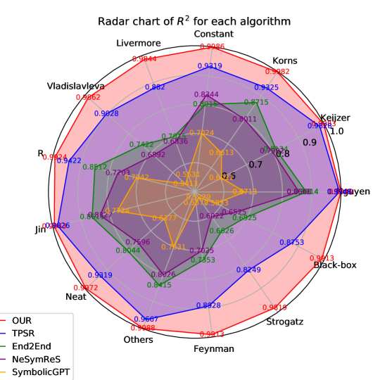
Figure 1: From the radar chart, we can see that the comprehensive performance of our algorithm achieves the state of the art on each data set.

1 Introduction

Symbolic Regression (SR) aims to identify the explicit mathematical expression underlying the observed data. Formally, for a given dataset $D=\{X,y\}$, SR seeks a function $f$ that satisfies $y=f(X)$, where $X\in\mathbb{R}^{n\times d}$, $y\in\mathbb{R}^{n}$, $d,n$ are the dimension of variable and number of data points, respectively. $f$ is composed of several basic primitive operators such as $+,-,\times,\div$, etc. SR has been applied in many fields, for example, material sciences(Wang et al., 2019), physical law exploration(Udrescu & Tegmark, 2020)(Udrescu et al., 2020)(Schmidt & Lipson, 2009), etc.

Genetic Programming Symbolic Regression (GPSR) has dominated in the past. GPSR uses the pre-order traversal of expression and acts as genes, and genetic operations such as mutation and crossover are used to produce descendants. Constants are randomly generated or optimized with the PSO algorithm. Although they have shown distinguished performances in several public benchmarks, they are sensitive to hyperparameters (Petersen, 2019) and the complexity of the learned expression tends to be high with the epoch increased.

With the huge success gained by deep learning in multiple domains (Alec et al., 2018), some works apply the deep learning technique in SR. EQL (Kim et al., 2021a) first substitutes the activation function of a fully connected feedforward neural network and refines the expression with Lasso. However, EQL is hard to tackle the division operation because it would generate exaggerated gradients in backpropagation. Therefore, DSR (Petersen, 2019) utilizes an RNN to emit the skeleton of expressions, constants are represented with a constant placeholder and optimized later by SGD. The risk-seeking policy gradients are used to update the RNN. To step further, DSO (Mundhenk et al., 2021) incorporates genetic programming into the search: RNN provides a better population for genetic programming algorithms. By doing so, DSO achieves remarkable results in SRBench (La Cava et al., 2021), Since the efficiency of reinforcement learning is lower than that of numerical optimization, MetaSymNet(Li et al., 2023) skillfully uses numerical optimization problem to solve the combinatorial optimization problem of symbolic regression.

The above-stated methods belong to the end-to-end model which trains a new model for each problem. This type of training strategy makes their search time long. Plus, the model can’t make full use of the search experiences from other searches. Therefore, the large-scale pre-trained model is proposed to improve the search speed. Normally, the large-scale pre-trained models (Valipour et al., 2021)(Luca et al., 2021)(Vastl et al., 2022) are trained with enormous self-generated data which contains the pairwise of sampled data points and corresponding mathematical expressions. The neural network has an encoder-decoder structure, the encoder maps the input data points into data features and the decoder uses the feature to generate the pre-order traversal of expressions. The Beam Search (Kumar et al., 2013) technique is applied to produce multiple candidate skeletons. Then, Broyden-Fletcher-Goldfarb-Shanno (BFGS) (Liu & Nocedal, 1989) is used to optimize the constants of candidate skeletons. Finally, the best-performed expression is selected as the final result.

The large-scale pre-trained model gained fast search speed because once the model finished training, we only needed a single forward pass to get the expressions. However, they ignore the different data formats of the input and output of SR. That is, previous methods treat the SR as a machine translation task: translate the data points into corresponding expressions. However, it is clear that the input and output of SR are very different from the two languages in translation, and they do not have an obvious word correspondence like languages. They are more like two different modalities (like image and text). Therefore, it is perhaps more reasonable to think of SR as a multimodal task.

To tackle the problems of two different modalities, we use a modal alignment module in our Transformer to make the encoded data feature close to the skeleton feature. We name our model as MMSR. Specifically, we use the SetTransformer (Lee et al., 2019) as a data encoder for it presents permutation invariance. And, decodes the skeleton of expression with a causal masking transformer decoder. Unlike standard decoder transformers, MMSR omits cross-attention in the first half of the decoder layers to encode unimodal skeleton representations, and cascades the rest of the decoder layers, cross-attending to the data encoder for multimodal data-skeleton representations. We use contrastive learning (Chuang et al., 2020) to align the modal features, so that the matching data features and skeleton features are as close as possible in the feature space, and the non-matching features are as far away from each other as possible. Additionally, we train the model with two extra losses: the cross-entropy loss used for predicting the token of expression skeletons. Second, one of the limitations of pre-train models is that they focus on the supervised pretraining goals borrowed from symbol generation, i.e., they are trained solely with the token-level cross-entropy (CE) loss, which can result in equations that may exhibit high token-level similarities but are suboptimal with respect to equation-specific objectives such as fitting accuracy(Shojaee et al., 2024). To solve this problem, we directly predict the numerical value of the constants and use MSE to measure the loss between the predicted constants and the true constants in the skeletons. We summarize our contributions as follows:

• We try to treat the symbolic regression task as a purely multimodal task according to the characteristics of the input and output of symbolic regression. And, a single end-to-end training session suffices to directly generate satisfactory outcomes.

• We introduce a modality alignment method so that the matched data features and skeleton features in the feature space can be as close as possible, and the mismatched features can be as far away as possible. To facilitate the later feature fusion. In particular, our contrastive loss and cross-entropy loss are both done in one step instead of separately trained. Experiments show that this can better promote the fusion of features.

• We conducted plenty of experiments and the results showed that the proposed model achieved state-of-the-art performances against the benchmarks.

The rest of the paper is organized as follows: Section 2 introduces the relevant research of our work, Section 3 describes the model structure, Section 4 lists the experiment settings and displays the experiment results, experiment analysis is also included. Finally, Section 5 gives a discussion and conclusion of our work.

2 Related Works

2.1 Multimodal

Recently, models such as CLIP (Radford et al., 2021) and ALIGN (Jia et al., 2021) performed pre-train on noisy images and text pairs from the web using contrastive loss. Contrastive loss is one of the most effective feature learning methods(He et al., 2020)(Chen et al., 2020)(Li et al., 2020b)(Li et al., 2020a). They achieve remarkable performance on image-text retrieval tasks but lack the ability to model more complex interactions between image and text for other V+L tasks (Kim et al., 2021b). (e.g. VQA(Antol et al., 2015)). Subsequent investigations (Wang et al., 2021) (Wang et al., 2022) (Piergiovanni et al., 2022) have introduced encoder-decoder frameworks trained utilizing generative loss functions, which demonstrate robust performance across vision-language benchmarks. Concurrently, the visual encoders within these models maintain competitive accuracy in image classification tasks. Studies (Singh et al., 2022) (Li et al., 2021) (Li et al., 2022a)(Chen et al., 2023)(Liu et al., 2024) have investigated the unification of image and text representations, which require multiple pretraining stages of unimodal and multimodal modules to achieve high-performance levels. For example, ALBEF (Li et al., 2021) employs a dual-encoder architecture that integrates contrastive loss with Masked Language Modeling (MLM) to enhance learning efficiency. CoCa(Yu et al., ) focuses on training an image-text foundation model from scratch in a single pretraining stage to unify these approaches. This is simpler and more efficient to train.

2.2 Deep Symbolic Regression

Before the explosion of deep symbolic regression methods, Genetic Programming Symbolic Regression (GPSR) (Arnaldo et al., 2014)(McConaghy, 2011)(Nguyen et al., 2017)(Zhang et al., 2021) was the main strategy for solving symbolic regression tasks. GPSR encodes the pre-order traversal of mathematical expression as the gene type, by randomly initializing a population of individuals, GPSR generates the candidate set of expressions. Then, it uses a fitness function to evaluate the fitting results, and genetic operations such as mutation and crossover are applied to produce new generations. The algorithm iterates until reaches the expected fitness value or the pre-defined maximum iteration epoch. Although GPSR could perform well in public benchmarks, it is reported to be sensitive to hyperparameters (Petersen, 2019). Furthermore, the GP-based method lacks an effective way to determine the constant value in the expression.

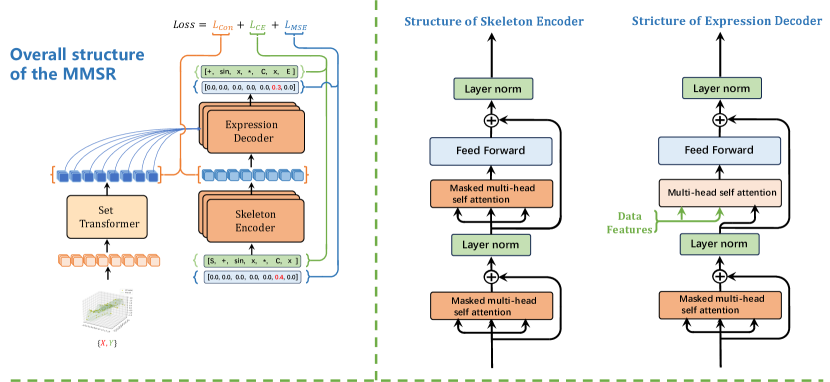
Figure 2: Our model’s framework.

With the huge success achieved by deep learning in various domains, EQL (Equation Learner) revised the activation functions of fully connected neural networks to primitives (sin, cos, etc.) and obtained the skeleton and constants through Lasso (Tibshirani, 1996) technique. However, the nontraditional activation functions cause troubles to the backpropagation process: the division operator would cause infinite gradients thus making the weights updating hard to continue. Moreover, the primitive sin, cos are periodical, and log, sqrt are not differentiable everywhere. DSR (Petersen, 2019) takes another learning strategy: it learns the skeleton first and optimizes the constants later. DSR uses an RNN to emit the probability distribution of the pre-order traversal, and autoregressively sample expressions according to the distribution. For gradient information lost in the sampling process, reinforcement learning is applied to update the RNN. Specifically, the risk-seeking policy gradients are used. Furthermore, to utilize the strong ability to generate new performed well expressions of GPSR, DSO (Mundhenk et al., 2021) incorporating the DSR and GPSR method to achieve state-of-the-art performance in SRBench. The RNN could provide a better population for GPSR to produce new descendants.

DSO is a type of learning-from-scratch method, it needs to train a new model for every problem. This training strategy comes with a huge search time cost. Thus, many learning-with-experience methods are emerged. They usually employ a data encoder to receive the data points as inputs and output the expression encoding as the label to train a large-scale model. When a new problem needs to be handled, the learning-with-experience method just implements a forward propagation to obtain the expressions thus being time-effective. SymbolicGPT (Valipour et al., 2021) treats the problem as a natural language problem, it uses symbolic-level encoding as the label of a set of data points. For example, the expression $2sin(x+y)$ is represented as text $[^{\prime}2^{\prime},^{\prime}s^{\prime},^{\prime}i^{\prime},^{\prime}n^{\prime},^{\prime}(^{\prime},^{\prime}x^{\prime},^{\prime}+^{\prime},^{\prime}y^{\prime},^{\prime})^{\prime}]$. This type of encoding forces the model to learn the syntax and semantics of the primitives thus increasing the learning difficulty. To free the model from learning the syntax and semantics meaning of primitives, NeSymReS (Luca et al., 2021) utilizes the pre-order traversal of binary tree to encode the expression. The constants in the expression are replaced with a placeholder “$c$” and optimized later after the skeleton is sampled according to the probability distribution outputted by the network. The pre-trained large-scale models have fast inference speed to obtain the predicted expression when confronted with new SR problems. The critical challenge of the SR task lies in two aspects: determining the skeleton and optimizing the constants. The above-stated large-scale pre-trained model could do well in predicting the skeleton, however, they normally use BFGS to optimize the constants which are sensitive to initial guesses. Therefore, to determine the constants accurately, based on the NeSymRe framework, Symformer (Vastl et al., 2022) and End2End (Kamienny et al., 2022) design two types of constant encoding strategies to teach the pre-trained model the exact value of constants. They perform with outstanding fitting accuracy than NeSymReS. Beyond the constant optimizing problem, Li et al (Li et al., 2022b) uses the Intra-class contrastive loss to train a better data encoder to tackle the ill-posed problem in SR. UDSR (Landajuela et al., 2022), SNR (Liu et al., 2023), and DGSR(Holt et al., 2023) merged multiple learning strategies to give the pre-trained model a revised mechanism. Moreover, the Monte Carlo Tree Search (Browne et al., 2012) is incorporated into the pre-trained model to achieve better performances.e.g.(Li et al., 2024). However, all the works view the SR task as a machine translation task that considers the input and output of the pre-trained model are the same data type. They ignore the fact that the data points are set data and the expression label is text. Thus, our work designs new architecture to solve the modality problem. SNIP(Meidani et al., 2023) employs a two-stage strategy to train a symbolic regression model. We pre-train an encoder using contrastive learning and then train a decoder separately. Since the two-stage training strategy is not conducive to feature fusion, SNIP also needs to introduce the LSO method to work well.

3 Method

3.1 Architecture

As depicted in Figure 2, the MMSR consists of two transformer-based encoders, each tailored for learning the symbolic or data representations of mathematical functions. Except that, a decoder receives the encoded numeric representations to decode the features to mathematical expressions. Additionally, an alignment module is designed to match the feature representations of numeric inputs and symbolic inputs. The contrastive learning (Chuang et al., 2020) is used to make the distance between the data and expression skeleton features that are derived from the same expression closer. During training, MMSR receives synthetically created symbolic equations and their associated numeric data as inputs to the symbolic encoder and numeric encoder, respectively. In total, MMSR is trained on approximately 10 million synthetic paired (numeric, symbolic) examples.

3.1.1 Data Encoder

Considering the permutation invariance of the data feature: it should maintain the same feature with the order change of data input. We thus applied SetTransformer (Lee et al., 2019) to be our data encoder. The input to the encoder consists of the data points $\mathcal{D}=\{X,y\}\in\mathbb{R}^{n\times d}$, which are first passed through a trainable affine layer to project them into a latent space $h_{n}\in\mathbb{R}^{d_{h}}$. The resulting vectors are then passed through several induced set attention blocks (Lee et al., 2019), which are several cross-attention layers. First, cross-attention uses a set of trainable vectors as the queries and the input features as keys and values. Its output is used as the keys and values for the second cross attention, and the original input vectors are used as the queries. After these cross-attention layers, we add a dropout layer (Srivastava et al., 2014). In the end, we compute cross attention between a set of trainable vectors (queries) to fix the size of the output such that it does not depend on the number of input points.

3.1.2 Expression Skeleton Encoder

Symbolic expression by $[+,-,*,/,sin,cos,exp,log\\ sqre,C-1,C-2,...,C4,C5,x_{1},x_{2},...]$ and other basic operators, where [C-5,…,C5] represents a constant placeholder. Each expression can be represented by an expression binary tree, and we can get a symbol sequence by expanding the expression binary tree in preorder. Furthermore, we treat each symbol as a $token$ and then embed it.

In particular, to solve the problem that expressions may exhibit high token-level similarities but are suboptimal for equation-specific objectives such as fitting accuracy, which is caused by only using the cross-entropy loss between the generated sequence and the real sequence, we encode the expression symbol sequence and the constant sequence separately. For example, for the expression $0.021*sin(x)+12.2$, we would have the symbolic sequence $[+,*,sin,x,C-1,C2]$. And constant sequence $[0,0,0,0.21,0.122]$. It is worth noting that we replace constants with special symbols. The constants are encoded using a scientific-like notation where a constant C is represented as a tuple of the exponent $c_{e}$ and the mantissa $c_{m}$, $C=c_{m}10^{c_{e}}$. Where $c_{e}$ belongs to integers between [-5,5] and $c_{m}$ belongs to [-1,1]. For example, for the constant 0.021 above, we use the placeholder C-1 in the skeleton, where $c_{m}$ is equal to 0.21 and $c_{e}$ is equal to -1, so $0.021=0.21*10^{-1}$

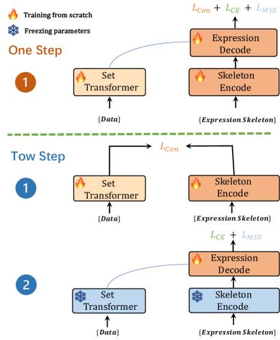
Figure 3: From the above five plots, we can see that as the size of the training data increases, the performance of the model on each dataset continues to improve. When the data size reaches 10M, the model has achieved satisfactory results on the selected data sets, and the average $R^{2}$ on each data set is greater than 0.98.

When calculating the loss function during training, we will calculate the cross-entropy loss for the predicted and true symbol sequences, and the numerical MSE loss for the predicted and true constant sequences. Note that when calculating the loss, we pad both the skeleton of the expression and the corresponding constants sequence to the maximum allowed length N, where the letter P is used for symbols and 0.0 is used for constants.

3.1.3 Expression Decoder

The decoder autoregressively generates the symbols sequence and the constants sequences given the encoder’s feature. We can think of each token as a token in a text generation task. Then, n candidate expressions are obtained by sampling sequentially using beam search according to the predicted probability distribution of the next symbol. And we’ll get n constants sequences corresponding to n skeletons of expressions. Next, the constant placeholder ‘[C-5,…, C5]’ in the skeleton is replaced by the corresponding constant to obtain the expression with the rough constant. Finally, we fine-tune the rough constant with BFGS to obtain the optimal expression.

3.1.4 Alignment Module

In the multimodal field, to make the features mapped by the matching modes close, to facilitate the subsequent multimodal feature fusion, to achieve better results. Contrastive loss is introduced in mainstream multimodal models to make the matched data features and skeleton features closer to each other, and the mismatched ones far away from each other in the feature space. Specifically, we align the features of the data obtained by the data point feature extraction extractor with the skeleton features obtained by the skeleton feature extractor. For the data point features, we will get the features of $\mathbb{R}^{b\times k\times h}$ for each batch, where $b$ stands for batch size and $k\times h$ represents the feature size obtained for each data. To facilitate the comparison loss later, we will map the features obtained from each batch from $\mathbb{R}^{b\times k\times h}$ to $\mathbb{R}^{b\times h}$. Similarly, we perform a similar operation for the skeleton feature. Then, the comparison loss is calculated for multiple data and skeleton samples contained in a Batch, and the similarity between positive samples (paired data and skeleton) is expected to be as high as possible, and the similarity between negative samples (unpaired data and skeleton) is expected to be as low as possible. The contrastive loss is formulated as follows.

$$\mathcal{L}_{Con}= -\frac{1}{N}\left(\sum_{i}^{N}\log\frac{\exp(x_{i}^{T}y_{i}/\theta)}{\sum_{j=1}^{N}\exp(x_{i}^{T}y_{i}/\theta)}\right.$$ (1)

$$\left.+\sum_{i}^{N}\log\frac{\exp(y_{i}^{T}x_{i}/\theta)}{\sum_{j=1}^{N}\exp(y_{i}^{T}x_{i}/\theta)}\right)$$

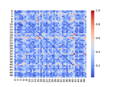
(a)

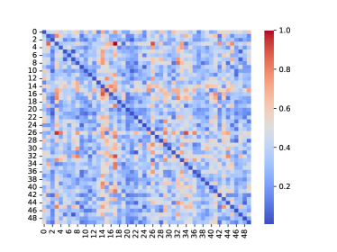
(b)

Figure 4: As we can see from the figure, under the premise that other configurations are completely the same, before the introduction of contrastive learning (Figure a), the cosine distance between the matched data features and the skeleton features extracted by the model in the feature space is not significantly smaller than that of the unmatched ones (the values on the diagonal are not significantly smaller than the others). However, after introducing contrastive learning (Figure b), we can clearly see that the values on the diagonal are significantly smaller than the values at other positions. That’s what we expected.

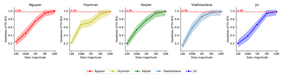
Figure 5: From the above five plots, we can see that as the size of the training data increases, the performance of the model on each dataset continues to improve. When the data size reaches 10M, the model has achieved satisfactory results on the selected data sets, and the average $R^{2}$ on each data set is greater than 0.98.

3.2 Training Objective

The loss function plays a crucial role in directing the training process of deep neural networks, which is imperative for effective deep learning. Our chosen loss function is composed of three components: cross-entropy loss ($L_{CE}$), mean squared error(MSE) loss ( $L_{MSE}$ ), and contrastive loss ( $L_{CON}$ ).

$$\mathcal{L}=\lambda_{1}\mathcal{L_{CE}}+\lambda_{2}\mathcal{L_{MSE}}+\lambda_{3}\mathcal{L_{CON}}$$ (2)

Here, $\mathcal{L_{CE}}$ represents the cross-entropy loss between the predicted expression sequence and the true sequence. $\mathcal{L_{MSE}}$ represents the MSE loss of the true constants and the predicted constants. $\mathcal{L_{CON}}$ represents the contrastion loss over a batch of samples, which is used to make the data features and expression features that match in the feature space closer to each other, and vice versa. $\lambda_{1}$ $\lambda_{2}$ $\lambda_{3}$ are hyperparameters that allow us to adjust the proportion of the three losses.

Table 1: Comparison of the number of nodes and parameters used by MetaSymNet and MLP when the $R^{2}$ is greater than 0.99.

Benchmark	Contrastive loss ($\mathcal{L_{CON}}$)
	$\lambda_{2}=1.0$	$\lambda_{2}=0.1$	$\lambda_{2}=0.0$
Nguyen	0.9999	0.9994	0.9701
Keijzer	0.9983	0.9724	0.9605
Korns	0.9982	0.9842	0.9364
Constant	0.9986	0.9024	0.8883
Livermore	0.9844	0.9388	0.9034
Vladislavleva	0.9862	0.9603	0.9242
R	0.9924	0.9831	0.9683
Jin	0.9943	0.9711	0.9422
Neat	0.9972	0.9633	0.9248
Others	0.9988	0.9555	0.9146
Feynman	0.9913	0.9735	0.9644
Strogatz	0.9819	0.9533	0.9272
Black-box	0.9913	0.9655	0.9028
Average	0.9932	0.9633	0.9328

4 Experiments

4.1 Dataset

In order to test the performance of MMSR and baselines, we conducted comparative analyses using prevalent datasets, designated as ’Nguyen’, ’Keijzer’, ’Korns’, ’Constant’, ’Livermore’, ’Vladislavleva’, ’R’,’ Jin’, ’Neat’,’ Others’, ’Feynman’, ’Strogatz’ and ’Black-box’. The three datasets Feynman ’, ’Strogatz’ and ’Black-box’ are from the SRbetch dataset. These datasets contain nearly 400 expressions in total. We believe that they can accurately and comprehensively test the performance of each algorithm.

4.2 Compared with State-of-the-arts

In order to test the performance of our algorithm against similar algorithms, we selected some representative ”pre-training-based” symbolic regression algorithms in recent years.

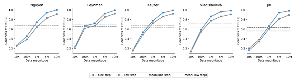
Figure 6: From the above five plots, we can see that as the size of the training data increases, the performance of the model on each dataset continues to improve. When the data size reaches 10M, the model has achieved satisfactory results on the selected data sets, and the average $R^{2}$ on each data set is greater than 0.98.

• SymbolicGPT: The classical algorithm for pre-trained models, which treats the symbolic regression problem as a translation problem. Treat a ‘single letter’ (e.g. ‘s’, ‘i’, ‘n’) as a token. Generating expressions sequentially.

• NeSymReS: Based on SymbolicGPT, the algorithm treated each ‘operator’ (e.g. ‘sin’, ‘cos’) as a token. The sequence of expressions is generated in turn. The setup is more reasonable.

• End2End: End2End further encodes the constants so that the model generates the constants directly when generating the expression, abandoning the constant placeholder ‘C’ used by the previous two algorithms.

• TPSR: One uses a pre-trained model as a policy network to guide the MCTS process, which greatly improves the search efficiency of MCTS.

The radar chart in Figure.1 shows the performance comparison between our algorithm and four baselines intuitively. From the figure, we can find that MMSR has a better fitting performance than the four baselines.

4.3 Ablation Study

To verify whether the introduction of contrastive learning plays a positive role in the algorithm performance, we conduct the ablation experiment as follows. On the premise of ensuring that the training data and other factors are exactly the same, According to Equation 2, we did three sets of experiments, in which $\lambda_{1}$ and $\lambda_{3}$ were always equal to 1, and $\lambda_{2}$ was set to 0.0, 0.1, and 1.0 in turn. The specific experimental results are shown in Table 1.

This can be clearly seen from the table. Other conditions being equal, as the proportion of contrastive learning loss ($\mathcal{L_{CON}}$) decreases gradually, the performance of the algorithm also decreases gradually. In addition, the overall performance with the contrastive loss (lambda2 = 1.0 and 0.1) is better than without the contrastive loss (lambda = 0.0).

4.4 Effects of modality alignment

In order to verify whether the extracted features before and after the introduction of contrastive learning are as expected: Data and skeleton features that match each other are close to each other in the feature space, whereas those that do not match are far away from each other. We first randomly generate 50 expression samples, feed these samples into the model without contrastive learning, and then obtain 50 pairs of features for the data and skeleton. We calculate the cosine distance between the extracted 50 data features and 50 skeleton features and then obtain the 50*50 cosine distance matrix A. Finally, we normalize the matrix A and visualize it to get fig 4(a). Similarly, we feed these samples into a model that uses contrastive learning, resulting in heatmap 4(b).

From figure 4, we can see that there is indeed a large change in the extracted features before and after the introduction of contrastive learning. In Figure 4(a), we can see that the data on the diagonal is not significantly smaller than the other positions, indicating that the matching data features and skeleton features are not the closest to each other in the feature space. On the contrary, we can clearly find in Figure 3b that the data on the diagonal is significantly smaller than the other positions, which indicates that our contrastive learning plays a role. The features of the two modalities, data and skeleton, have been well aligned.

4.5 Impact of the size of the training data

To test the impact of pre-training data on model test performance, we train our MMSR model on increasingly larger datasets. More specifically, we use datasets consisting of 10K, 100K, 1M, 5M, and 10M samples to train a model respectively. Except for the amount of data, every other aspect of training is the same as described above, and all are trained for the same epochs.

From the trend in Figure 5, we can see that the performance of the model has been greatly improved as the data set continues to grow. We can see that when the data size reaches 5M, the average $R^{2}$ has reached more than 0.9, and when the data size reaches 10M, The model achieves an average $R^{2}$ of over 0.98 on each dataset. Although the growth rate of average $R^{2}$ is relatively slow with the increase of data, it is still increasing. Therefore, it can be inferred that as we continue to increase the size of the training data, the performance of the model will still reach higher levels.

4.6 Effect of the introduction method of contrastive learning

It is very important to use contrastive learning for modality alignment in multi-modality. At present, there are two methods to introduce contrastive learning:

• One step. The contrast loss is used as a part of the total loss, and the feature extraction module and the feature fusion module are trained at the same time.

• Tow step. First, train a feature extraction module with contrastive learning, then freeze it, and then train a feature fusion module separately.

Figure.LABEL:fig7 shows the comparison plot between the One step strategy and the Tow step strategy. To prove the superiority of our adopted strategy, we conduct comparative experiments on five datasets. From figure 6, we can find that in terms of contrastive learning introduction method, the One-step strategy we adopted is slightly better than the Tow-step strategy in terms of effect. As the size of the dataset increases, this advantage becomes more and more obvious.

We believe that the specific reason for this phenomenon is that in the One-step strategy, contrastive loss and other losses are trained together. In the process of training, the feature extraction module and the feature fusion module are interrelated. This requires the feature extraction module not only to make the extracted data and skeleton features close in the feature space but also to make the extracted features better adapt to the later feature fusion module. So that the overall loss is smaller. In short, the one-step strategy can make each module better fit each other in the process of training together.

5 Discussion and conclusion

In this paper, we propose a symbolic regression algorithm, MMSR. We solve the SR problem as a purely multimodal problem and obtain decent experimental results. This also proves that it is practical to treat the SR problem as a multimodal task. Specifically, we treat the data and expression skeleton as two different modalities (e.g. image and text). For the data part, we use SetTransformer for the feature extractor, and for the expression skeleton part, we use the first few layers of the transformer as the feature extractor. Specifically, we introduce contrastive learning for modal feature alignment for better feature fusion. The ablation experiments on more than a dozen datasets show that the introduction of contrastive learning has a great improvement in the performance of the algorithm. In addition, we adopt the One-step scheme(the contrastive loss is trained along with other losses during training) in MMSR. Our experiments show that the One-step scheme is more competitive than the Tow-step scheme, which first trains a feature extraction module with contrastive loss and then trains the feature fusion module separately. In MMSR, alleviating expressions may exhibit high token-level similarities but are suboptimal with respect to equation-specific objectives such as fitting accuracy. Our decoder not only generates the sequence of symbols that make up the skeleton of an expression but also directly generates a set of constants. This set of constants is the same length as the symbol sequence, we take the constant with the same index as the placeholder ’C’ as the value at ’C’, and then the constants are further refined with BFGS to obtain the final expression.

Our algorithm is expected to open new application prospects of multimodal technology. It promotes more multimodal correlation techniques to be applied to the field of symbolic regression. We can even use symbolic regression techniques to re-feed multi-modal domains.

At present, although MMSR has achieved good results, it also has many imperfect. For example, its anti-noise performance is poor. The type of symbol used cannot be changed once the training is complete. The maximum number of support variables must also be specified in advance and cannot be expanded once the training is complete.

Next, we will continue to explore the deep fusion of multimodal techniques and symbolic regression techniques. It also attempts to solve some of the existing problems of MMSR mentioned above.

References

- Alec et al. (2018) Alec, R., Karthik, N., Tim, S., and Ilya, S. Improving language understanding by generative pre-training. 2018.
- Antol et al. (2015) Antol, S., Agrawal, A., Lu, J., Mitchell, M., Batra, D., Zitnick, C. L., and Parikh, D. Vqa: Visual question answering. In Proceedings of the IEEE international conference on computer vision, pp. 2425–2433, 2015.
- Arnaldo et al. (2014) Arnaldo, I., Krawiec, K., and O’Reilly, U.-M. Multiple regression genetic programming. In Proceedings of the 2014 Annual Conference on Genetic and Evolutionary Computation, pp. 879–886, New York, NY, USA, 2014. Association for Computing Machinery. ISBN 9781450326629. doi: 10.1145/2576768.2598291. URL https://doi.org/10.1145/2576768.2598291.
- Browne et al. (2012) Browne, C. B., Powley, E., Whitehouse, D., Lucas, S. M., Cowling, P. I., Rohlfshagen, P., Tavener, S., Perez, D., Samothrakis, S., and Colton, S. A survey of monte carlo tree search methods. IEEE Transactions on Computational Intelligence and AI in games, 4(1):1–43, 2012.
- Chen et al. (2020) Chen, T., Kornblith, S., Norouzi, M., and Hinton, G. A simple framework for contrastive learning of visual representations. In International conference on machine learning, pp. 1597–1607. PMLR, 2020.
- Chen et al. (2023) Chen, X., Djolonga, J., Padlewski, P., Mustafa, B., Changpinyo, S., Wu, J., Ruiz, C. R., Goodman, S., Wang, X., Tay, Y., et al. Pali-x: On scaling up a multilingual vision and language model. arXiv preprint arXiv:2305.18565, 2023.
- Chuang et al. (2020) Chuang, C.-Y., Robinson, J., Lin, Y.-C., Torralba, A., and Jegelka, S. Debiased contrastive learning. Advances in neural information processing systems, 33:8765–8775, 2020.
- He et al. (2020) He, K., Fan, H., Wu, Y., Xie, S., and Girshick, R. Momentum contrast for unsupervised visual representation learning. In Proceedings of the IEEE/CVF conference on computer vision and pattern recognition, pp. 9729–9738, 2020.
- Holt et al. (2023) Holt, S., Qian, Z., and van der Schaar, M. Deep generative symbolic regression. arXiv preprint arXiv:2401.00282, 2023.
- Jia et al. (2021) Jia, C., Yang, Y., Xia, Y., Chen, Y.-T., Parekh, Z., Pham, H., Le, Q., Sung, Y.-H., Li, Z., and Duerig, T. Scaling up visual and vision-language representation learning with noisy text supervision. In International conference on machine learning, pp. 4904–4916. PMLR, 2021.
- Kamienny et al. (2022) Kamienny, P.-A., d’Ascoli, S., Lample, G., and Charton, F. End-to-end symbolic regression with transformers. Advances in Neural Information Processing Systems, 35:10269–10281, 2022.
- Kim et al. (2021a) Kim, S., Lu, P. Y., Mukherjee, S., Gilbert, M., Jing, L., Čeperić, V., and Soljačić, M. Integration of neural network-based symbolic regression in deep learning for scientific discovery. IEEE Transactions on Neural Networks and Learning Systems, 32(9):4166–4177, 2021a. doi: 10.1109/TNNLS.2020.3017010.
- Kim et al. (2021b) Kim, W., Son, B., and Kim, I. Vilt: Vision-and-language transformer without convolution or region supervision. In International Conference on Machine Learning, pp. 5583–5594. PMLR, 2021b.
- Kumar et al. (2013) Kumar, A., Vembu, S., Menon, A. K., and Elkan, C. Beam search algorithms for multilabel learning. Machine learning, 92:65–89, 2013.
- La Cava et al. (2021) La Cava, W., Orzechowski, P., Burlacu, B., de França, F. O., Virgolin, M., Jin, Y., Kommenda, M., and Moore, J. H. Contemporary symbolic regression methods and their relative performance. arXiv preprint arXiv:2107.14351, 2021.
- Landajuela et al. (2022) Landajuela, M., Lee, C. S., Yang, J., Glatt, R., Santiago, C. P., Aravena, I., Mundhenk, T., Mulcahy, G., and Petersen, B. K. A unified framework for deep symbolic regression. Advances in Neural Information Processing Systems, 35:33985–33998, 2022.
- Lee et al. (2019) Lee, J., Lee, Y., Kim, J., Kosiorek, A., Choi, S., and Teh, Y. W. Set transformer: A framework for attention-based permutation-invariant neural networks. In Proceedings of the 36th International Conference on Machine Learning, volume 97 of Proceedings of Machine Learning Research, pp. 3744–3753. PMLR, 09–15 Jun 2019. URL https://proceedings.mlr.press/v97/lee19d.html.
- Li et al. (2020a) Li, J., Xiong, C., and Hoi, S. C. Mopro: Webly supervised learning with momentum prototypes. arXiv preprint arXiv:2009.07995, 2020a.
- Li et al. (2020b) Li, J., Zhou, P., Xiong, C., and Hoi, S. C. Prototypical contrastive learning of unsupervised representations. arXiv preprint arXiv:2005.04966, 2020b.
- Li et al. (2021) Li, J., Selvaraju, R., Gotmare, A., Joty, S., Xiong, C., and Hoi, S. C. H. Align before fuse: Vision and language representation learning with momentum distillation. Advances in neural information processing systems, 34:9694–9705, 2021.
- Li et al. (2022a) Li, J., Li, D., Xiong, C., and Hoi, S. Blip: Bootstrapping language-image pre-training for unified vision-language understanding and generation. In International Conference on Machine Learning, pp. 12888–12900. PMLR, 2022a.
- Li et al. (2022b) Li, W., Li, W., Sun, L., Wu, M., Yu, L., Liu, J., Li, Y., and Tian, S. Transformer-based model for symbolic regression via joint supervised learning. In The Eleventh International Conference on Learning Representations, 2022b.
- Li et al. (2023) Li, Y., Li, W., Yu, L., Wu, M., Liu, J., Li, W., Hao, M., Wei, S., and Deng, Y. Metasymnet: A dynamic symbolic regression network capable of evolving into arbitrary formulations. arXiv preprint arXiv:2311.07326, 2023.
- Li et al. (2024) Li, Y., Li, W., Yu, L., Wu, M., Liu, J., Li, W., Hao, M., Wei, S., and Deng, Y. Discovering mathematical formulas from data via gpt-guided monte carlo tree search. arXiv preprint arXiv:2401.14424, 2024.
- Liu & Nocedal (1989) Liu, D. C. and Nocedal, J. On the limited memory bfgs method for large scale optimization. Mathematical programming, 45(1-3):503–528, 1989.
- Liu et al. (2024) Liu, H., Li, C., Wu, Q., and Lee, Y. J. Visual instruction tuning. Advances in neural information processing systems, 36, 2024.
- Liu et al. (2023) Liu, J., Li, W., Yu, L., Wu, M., Sun, L., Li, W., and Li, Y. Snr: Symbolic network-based rectifiable learning framework for symbolic regression. Neural Networks, 165:1021–1034, 2023.
- Luca et al. (2021) Luca, B., Tommaso, B., Alexander, N., Aurelien, L., and Giambattista, P. Neural symbolic regression that scales. In Proceedings of the 38th International Conference on Machine Learning, volume 139 of Proceedings of Machine Learning Research, pp. 936–945. PMLR, 2021.
- McConaghy (2011) McConaghy, T. FFX: Fast, Scalable, Deterministic Symbolic Regression Technology. Springer New York, New York, NY, 2011. ISBN 978-1-4614-1770-5. doi: 10.1007/978-1-4614-1770-5“˙13. URL https://doi.org/10.1007/978-1-4614-1770-5_13.
- Meidani et al. (2023) Meidani, K., Shojaee, P., Reddy, C. K., and Farimani, A. B. Snip: Bridging mathematical symbolic and numeric realms with unified pre-training. arXiv preprint arXiv:2310.02227, 2023.
- Mundhenk et al. (2021) Mundhenk, T. N., Landajuela, M., Glatt, R., Santiago, C. P., Faissol, D. M., and Petersen, B. K. Symbolic regression via neural-guided genetic programming population seeding. CoRR, abs/2111.00053, 2021. URL https://arxiv.org/abs/2111.00053.
- Nguyen et al. (2017) Nguyen, S., Zhang, M., and Tan, K. C. Surrogate-assisted genetic programming with simplified models for automated design of dispatching rules. IEEE Transactions on Cybernetics, 47(9):2951–2965, 2017. doi: 10.1109/TCYB.2016.2562674.
- Petersen (2019) Petersen, B. K. Deep symbolic regression: Recovering mathematical expressions from data via policy gradients. CoRR, abs/1912.04871, 2019. URL http://arxiv.org/abs/1912.04871.
- Piergiovanni et al. (2022) Piergiovanni, A., Li, W., Kuo, W., Saffar, M., Bertsch, F., and Angelova, A. Answer-me: Multi-task open-vocabulary visual question answering. arXiv preprint arXiv:2205.00949, 2022.
- Radford et al. (2021) Radford, A., Kim, J. W., Hallacy, C., Ramesh, A., Goh, G., Agarwal, S., Sastry, G., Askell, A., Mishkin, P., Clark, J., et al. Learning transferable visual models from natural language supervision. In International conference on machine learning, pp. 8748–8763. PMLR, 2021.
- Schmidt & Lipson (2009) Schmidt, M. and Lipson, H. Distilling free-form natural laws from experimental data. Science, 324(5923):81–85, 2009. doi: 10.1126/science.1165893. URL https://www.science.org/doi/abs/10.1126/science.1165893.
- Shojaee et al. (2024) Shojaee, P., Meidani, K., Barati Farimani, A., and Reddy, C. Transformer-based planning for symbolic regression. Advances in Neural Information Processing Systems, 36, 2024.
- Singh et al. (2022) Singh, A., Hu, R., Goswami, V., Couairon, G., Galuba, W., Rohrbach, M., and Kiela, D. Flava: A foundational language and vision alignment model. In Proceedings of the IEEE/CVF Conference on Computer Vision and Pattern Recognition, pp. 15638–15650, 2022.
- Srivastava et al. (2014) Srivastava, N., Hinton, G., Krizhevsky, A., Sutskever, I., and Salakhutdinov, R. Dropout: A simple way to prevent neural networks from overfitting. Journal of Machine Learning Research, 15(1):1929–1958, 2014.
- Tibshirani (1996) Tibshirani, R. Regression shrinkage and selection via the lasso. Journal of the Royal Statistical Society: Series B (Methodological), 58(1):267–288, 1996. doi: https://doi.org/10.1111/j.2517-6161.1996.tb02080.x.
- Udrescu & Tegmark (2020) Udrescu, S.-M. and Tegmark, M. Ai feynman: A physics-inspired method for symbolic regression. Science Advances, 6(16):eaay2631, 2020. doi: 10.1126/sciadv.aay2631.
- Udrescu et al. (2020) Udrescu, S.-M., Tan, A., Feng, J., Neto, O., Wu, T., and Tegmark, M. Ai feynman 2.0: Pareto-optimal symbolic regression exploiting graph modularity. In Advances in Neural Information Processing Systems, volume 33, pp. 4860–4871. Curran Associates, Inc., 2020.
- Valipour et al. (2021) Valipour, V., You, B., Panju, M., and Ghodsi, A. Symbolicgpt: A generative transformer model for symbolic regression. CoRR, abs/2106.14131, 2021. URL https://arxiv.org/abs/2106.14131.
- Vastl et al. (2022) Vastl, M., Kulhánek, J., Kubalík, J., Derner, E., and Babuska, R. Symformer: End-to-end symbolic regression using transformer-based architecture. CoRR, abs/2205.15764, 2022. doi: 10.48550/arXiv.2205.15764. URL https://doi.org/10.48550/arXiv.2205.15764.
- Wang et al. (2022) Wang, P., Yang, A., Men, R., Lin, J., Bai, S., Li, Z., Ma, J., Zhou, C., Zhou, J., and Yang, H. Ofa: Unifying architectures, tasks, and modalities through a simple sequence-to-sequence learning framework. In International Conference on Machine Learning, pp. 23318–23340. PMLR, 2022.
- Wang et al. (2019) Wang, Y., Wagner, N., and Rondinelli, J. M. Symbolic regression in materials science. MRS Communications, 9(3):793––805, 2019.
- Wang et al. (2021) Wang, Z., Yu, J., Yu, A. W., Dai, Z., Tsvetkov, Y., and Cao, Y. Simvlm: Simple visual language model pretraining with weak supervision. arXiv preprint arXiv:2108.10904, 2021.
- (48) Yu, J., Wang, Z., Vasudevan, V., Yeung, L., Seyedhosseini, M., and Wu, Y. Coca: Contrastive captioners are image-text foundation models. arxiv 2022. arXiv preprint arXiv:2205.01917.
- Zhang et al. (2021) Zhang, F., Mei, Y., Nguyen, S., and Zhang, M. Evolving scheduling heuristics via genetic programming with feature selection in dynamic flexible job-shop scheduling. IEEE Transactions on Cybernetics, 51(4):1797–1811, 2021. doi: 10.1109/TCYB.2020.3024849.