Analytic solutions for the linearized first-order magnetohydrodynamics and implications for causality and stability

Abstract

We solve the first-order relativistic magnetohydrodynamics (MHD) within the linear-mode analysis performed near an equilibrium configuration in the fluid rest frame. We find two complete sets of analytic solutions for the four and two coupled modes with seven dissipative transport coefficients. The former set has been missing in the literature for a long time. Our method provides a simple and general algorithm for the solution search on an order-by-order basis in the derivative expansion, and can be applied to general sets of hydrodynamic equations. We also find that the small-momentum expansions of the solutions break down when the momentum direction is nearly perpendicular to an equilibrium magnetic field due to the presence of another small quantity, that is, a trigonometric function representing the anisotropy. We elaborate on the angle dependence of the solutions and provide alternative series representations that work near the right angle. Finally, we discuss the issues of causality and stability based on our analytic solutions and recent developments in the literature.

1 Introduction

Relativistic magnetohydrodynamics (MHD) has been developing as a framework to describe various systems ranging from the femto-scale droplets realized in relativistic heavy-ion collisions at RHIC and LHC Inghirami:2016iru ; Inghirami:2019mkc ; Nakamura:2022idq ; Nakamura:2022wqr ; Nakamura:2022ssn to the cosmological/astronomical scales. The latter includes the accretion flows and jet formation near black holes McKinney:2008ev ; McKinney:2012vh ; Bromberg:2015wra ; Davis:2020wea , supernova explosions Shibata:2006hr ; Matsumoto:2020rbz ; Matsumoto:2022hzg , and the binary mergers of neutron stars (NSs) Duez:2005cj ; Shibata:2021bbj ; Shibata:2021xmo ; Kiuchi:2023obe and of NS-BH Etienne:2011ea ; Hayashi:2021oxy (see also references therein). More recent developments include observations of the magnetic inverse cascade with coupled dynamics of the magnetic helicity (and the fermion chirality) Boyarsky:2011uy ; Rogachevskii:2017uyc ; Brandenburg:2017rcb ; Schober:2017cdw ; Masada:2018swb ; DelZanna:2018dyb ; Matsumoto:2022lyb ; Schober:2021iws ; Brandenburg:2023aco ; Brandenburg:2023rrd ; Schober:2023zxl (see Refs. brandenburg2023chirality ; Kamada:2022nyt ; Hattori:2023egw for reviews).

In recent years, relativistic MHD was reformulated based on the conservation of the magnetic flux Grozdanov:2016tdf ; Hattori:2017usa ; Armas:2018atq ; Hongo:2020qpv (see Ref. Hattori:2022hyo for a review). On the other hand, the conventional formulation is based on a coupled system of the Maxwell equation and the energy-momentum conservation law, where both equations have the source terms stemming from the electric current and the Joule heat and Lorentz force, respectively. This implies the presence of non-conserved charges, i.e., gapped modes, involved in the conventional formulation. In fact, electric fields are damped out or screened when systems approach equilibrium states. The new formulation canonically follows the spirit of hydrodynamics, that is, conservation laws associated with symmetries. The magnetic flux conservation is identified as a consequence of generalized concept of global symmetries called the magnetic one-form symmetry Gaiotto:2014kfa .

In this paper, we focus on solving the set of MHD equations. We linearize the MHD equations with respect to perturbative disturbances applied to an equilibrium state and obtain the dispersion relations for the eigenmodes. This analysis, called the linear-mode analysis, has been conventionally used to discuss causality and stability of hydrodynamic theories Hiscock:1983zz ; Hiscock:1985zz ; Hiscock:1987zz (see below for recent progress on causality and stability analyses). While the linear-mode analysis was applied to the relativistic MHD in the recent literature Grozdanov:2016tdf ; Hernandez:2017mch ; Biswas:2020rps ; Armas:2022wvb , a complete set of solutions is still missing. The difficulty simply arises from the fact that one needs to diagonalize a large matrix in the absence of a spatial rotational symmetry broken by a magnetic field. In this paper, we develop an analytic algorithm for the solutions search on an order-by-order basis in the derivative expansion and obtain the complete set of analytic solutions. It is useful to obtain analytic solutions since the transport coefficients and the equations of state are often not (precisely) known in individual systems. Moreover, our method works as a general algorithm for the solution search, and can be applied to general sets of equations based on derivative expansions.

The complete set of solutions consists of six gappless modes, which are known as a pair of the Alfven waves and two pairs of the magneto-sonic waves. We fully include the first-order derivative corrections that consist of three bulk viscosities, two shear viscosities, and two electric resistivities. We focus on the Landau frame while a straightforward extension can be carried out for a general frame choice and general matching conditions of hydrodynamic variables (see, e.g., Ref. Hattori:2022hyo for discussions about these choices in MHD and Ref. Armas:2022wvb for a recent linear-mode analysis without a specific choice). In the presence of the anisotropic corrections, the solutions for the magneto-sonic modes had been only known in the two particular limits where the momentum is oriented parallel or perpendicular to a background magnetic field Grozdanov:2016tdf ; Hernandez:2017mch ; Armas:2022wvb .

We further discuss the convergence of the small-momentum expansion by inspecting the obtained solutions and find that the higher-order terms in the small-momentum expansion diverge when the momentum is taken nearly perpendicular to a magnetic field. This issue is caused by the presence of another small quantity, that is, a trigonometric function representing the angle dependence. We find this issue both in the Alfven and magneto-sonic modes. It can be a general issue in anisotropic systems. We identify the correct result obtained from the original equations before the small-momentum expansion is performed, giving a different result than that in the literature Grozdanov:2016tdf ; Armas:2022wvb . We provide an alternative series representation that correctly captures the anisotropy near the right angle.

Finally, we discuss the causality and stability of relativistic MHD. We show that the phase velocities, that are called the Alfven velocities and the fast and slow magneto-sonic velocities, are always smaller than the speed of light. This means that the linear waves are causal within the ideal MHD. We also show that the first-order corrections, obtained within the fluid rest frame, always provide damping effects on the linear waves as long as the transport coefficients satisfy the inequalities required by the second law of thermodynamics. This is expected since MHD only contains dissipative transport coefficients. The absence of growing modes indicates stability of an equilibrium state within the fluid rest frame where the linear-mode analysis is performed. However, those conditions are not sufficient to guarantee the causality and stability of dissipative hydrodynamics in general Lorentz frames. It has been widely know that diffusive modes are acausal, leading to developments of the Israel-Steward theory Israel:1976tn ; Israel:1978up ; Israel:1979wp (see, e.g., Ref. Denicol:2014loa for a review), and observers in different Lorentz frames could see (unphysical) unstable modes (see, e.g., Ref. Denicol:2008ha ).

Recent developments deepened our understanding of the issues of causality and stability. A stronger necessary condition for a stable dispersion relation was obtained from complex analysis of a retarded propagator in general causal theories Heller:2022ejw . Then, it was explicitly shown that, unless this necessary condition is satisfied, one finds a boost velocity that transforms a stable mode in the fluid rest frame to an unstable mode in the boosted frame Gavassino:2021owo ; Gavassino:2023myj . We briefly discuss a generalization of this crucial condition to anisotropic systems including MHD. The reader is referred to recent related works Bemfica:2017wps ; Bemfica:2019knx ; Bemfica:2020zjp ; Bemfica:2020xym Kovtun:2019hdm ; Hoult:2020eho Wang:2023csj that may be classified in terms of employed criteria for causality and stability; with or without specific choices of a flow vector and hydrodynamic variables; and with or without the linearization. One is demanded to perform more analyses when including more conserved charges such as a vector charge Brito:2020nou , magnetic field Biswas:2020rps ; Armas:2022wvb ; Cordeiro:2023ljz , axial charge Speranza:2021bxf ; Abboud:2023hos , and/or spin Daher:2022wzf ; Sarwar:2022yzs ; Weickgenannt:2023btk ; Xie:2023gbo .

This paper is organized as follows. We first recapitulate the recent formulation of relativistic MHD in Sec. 2 and show a set of linearized equations in Sec. 3. In Sec. 4, we introduce our method for the solution search. We elaborate on the convergence/breakdown of the small-momentum expansion. In Sec. 5, we discuss causality and stability of MHD, which is supported by Appendices. Finally, we conclude this paper in Sec. 6. Throughout the paper, we use the mostly plus metric convention ${\eta^{\mu\nu}}=\text{diag}(-1,1,1,1)$ and the completely antisymmetric tensor with the convention $\epsilon^{0123}=+1$. Then, the fluid velocity ${u^{\mu}}$ is normalized as ${u^{\mu}}{u_{\mu}}=-1$. We define the projection operator ${\Delta^{\mu\nu}}={\eta^{\mu\nu}}+{u^{\mu}}{u^{\nu}}$ such that $u_{\mu}\Delta^{\mu\nu}=0$. To specify the direction of a magnetic field, we introduce a spatial unit vector ${b^{\mu}}$ such that $b^{\mu}b_{\mu}=1$ and $u_{\mu}b^{\mu}=0$ and accordingly another projection operator ${\Xi^{\mu\nu}}={\Delta^{\mu\nu}}-{b^{\mu}}{b^{\nu}}$ such that $b_{\mu}\Xi^{\mu\nu}=0=u_{\mu}\Xi^{\mu\nu}$.

2 First-order MHD from the magnetic-flux conservataion

We recapitulate the formulation of relativistic MHD with the magnetic-flux conservation Grozdanov:2016tdf ; Hattori:2017usa ; Armas:2018atq ; Hongo:2020qpv (see Ref. Hattori:2022hyo for a review). While the magnetic flux is conserved in the absence of a magnetic monopole, the electric flux can terminate at electric charges, implying that an electric field is not a conserved quantity. The conservation laws for the energy-momentum tensor $\Theta^{\mu\nu}$ and the (dual) electromagnetic field strength tensor ${\tilde{F}}^{\mu\nu}=\frac{1}{2}\epsilon^{\mu\nu\rho\sigma}F_{\rho\sigma}$ read

$${\partial_{\mu}}{\Theta^{\mu\nu}}=0,\quad{\partial_{\mu}}{{\tilde{F}}^{\mu\nu}}=0.$$ (1)

Realizing the second equation as a conservation law for the magnetic flux led to a renewed formulation of magnetohydrodynamics along with the symmetry guideline, but with a generalized notion called the one-form symmetry.

The temporal components of the conserved currents provide the corresponding conserved charges

$$e=u_{\mu}u_{\nu}{\Theta^{\mu\nu}},\quad B^{\mu}=-{\tilde{F}}^{\mu\nu}u_{\nu}.$$ (2)

We postulate that these quantities satisfy the first law of thermodynamics

$$Ts = e+{p}-{H_{\mu}}{B^{\mu}},$$ (3a)

$$Tds = de-{H_{\mu}}d{B^{\mu}},$$ (3b)

$$TDs = De-{H_{\mu}}D{B^{\mu}},$$ (3c)

where we defined the temporal derivative $D=u^{\mu}\partial_{\mu}$. The translational symmetry of the system guarantees the conservation of the total energy density $e$ that contains not only matter contributions but also electromagnetic energy. The corresponding pressure $p$ should also be the total quantity.

To organize a closed system of equations, one needs to obtain the constitutive equations that express the spatial components of the conserved currents by the conserved charges. Based on the derivative expansion, the constitutive equations can be written down as

$${\Theta^{\mu\nu}} = e{u^{\mu}}{u^{\nu}}+{p_{\parallel}}{b^{\mu}}{b^{\nu}}+{p_{\bot}}{\Xi^{\mu\nu}}+\Theta_{(1)}^{\mu\nu},$$ (4a)

$${{\tilde{F}}^{\mu\nu}} = {B^{\mu}}{u^{\nu}}-{B^{\nu}}{u^{\mu}}+\tilde{F}_{(1)}^{\mu\nu},$$ (4b)

where we introduced a unit vector ${b^{\mu}}={B^{\mu}}/\sqrt{{B^{\nu}}{B_{\nu}}}$ and the projection operator ${\Xi^{\mu\nu}}={\Delta^{\mu\nu}}-{b^{\mu}}{b^{\nu}}$ such that $b_{\mu}\Xi^{\mu\nu}=0=u_{\mu}\Xi^{\mu\nu}$; Note that $u_{\mu}B^{\mu}=0$ by definition (2). The explicitly written terms exhaust the zeroth-order terms that can be constructed with the available tensors in the absence of the vector and axial charges. The subscripts denote the first-order corrections that will be constrained by the entropy-current analysis below.

We are in position to compute the divergence of the entropy current $s^{\mu}=su^{\mu}+s_{(1)}^{\mu}$, where $s_{(1)}^{\mu}$ is the first-order corrections to the entropy current. It can be expressed with the derivatives of the conserved quantities by the use of the first law of thermodynamics (3). Then, using the equations of motion (1) together with the constitutive equations (4), one finds that

$$\partial_{\mu}s^{\mu} = s\partial_{\mu}u^{\mu}+Ds+\partial_{\mu}s_{(1)}^{\mu}$$

$$= \beta(Ts-\epsilon-p_{\perp}+H_{\mu}B^{\mu})\partial_{\mu}u^{\mu}-\beta\big{[}\,(p_{\parallel}-p_{\perp})b^{\mu}b^{\nu}+Bb^{\mu}H^{\nu}\,\big{]}\partial_{\mu}u_{\nu}$$

$$-\Theta^{\mu\nu}_{(1)}\partial_{\mu}\beta_{\nu}+\tilde{F}^{\mu\nu}_{(1)}\partial_{\mu}(\beta H_{\nu})+\partial_{\mu}(s_{(1)}^{\mu}+\beta u_{\nu}\Theta^{\mu\nu}_{(1)}+\beta\omega_{\alpha\beta}\Sigma^{\mu\alpha\beta}_{(1)}-\beta H_{\nu}\tilde{F}^{\mu\nu}_{(1)}).$$

The leading-order terms in derivative describe the ideal MHD. For the entropy production to vanish at the ideal order, one should have

$$p_{\perp}=p,$$ (6a)

$$({p_{\parallel}}-{p_{\bot}}){b^{\nu}}+{H^{\nu}}B=0.$$ (6b)

The zeroth-order result can be summarized as

$$\Theta^{\mu\nu}_{(0)} = \epsilon u^{\mu}u^{\nu}-p\Xi^{\mu\nu}+(p-B_{\mu}H^{\mu})b^{\mu}b^{\nu},$$ (7)

where $H^{\mu}=\mu_{m}^{-1}B^{\mu}$ with $\mu_{m}$ being the magnetic permeability. The above result indicates the pressure anisotropy induced by the Maxwell stress.

The second law of thermodynamics requires that the first-order corrections be semi-positive definite. This condition is satisfied if individual contributions of thermodynamic forces take semi-positive values in Eq. (2), i.e.,

$$-\Theta_{(1)}^{\mu\nu}{\partial_{\mu}}{\beta_{\nu}}\geq 0,$$ (8a)

$$\tilde{F}_{(1)}^{\mu\nu}\partial_{\mu}(\beta{H_{\nu}})\geq 0.$$ (8b)

These inequalities can be insured for general hydrodynamic configurations if the left-hand sides are organized in bilinear forms, constraining the possible forms of the constitutive equations as

$$\Theta_{(1)}^{\mu\nu} = -T\eta^{\mu\nu\rho\sigma}\partial_{(\rho}\beta_{\sigma)},$$ (9a)

$$\tilde{F}_{(1)}^{\mu\nu} = -T\rho^{\mu\nu\rho\sigma}{\partial_{[\rho}}(\beta{H_{\sigma]}}).$$ (9b)

The fourth-rank tensors $\eta^{\mu\nu\rho\sigma}$ and $\rho^{\mu\nu\rho\sigma}$ can be constructed with the available tensors, $u^{\mu}$, $b^{\mu}$, $\Xi^{\mu\nu}$, and $\epsilon^{\mu\nu\alpha\beta}$, as Grozdanov:2016tdf ; Hongo:2020qpv ; Hattori:2022hyo

$${\eta^{\mu\nu\rho\sigma}} = \begin{pmatrix}b^{\mu}b^{\nu}&\Xi^{\mu\nu}\end{pmatrix}\begin{pmatrix}\zeta_{\parallel}&\zeta_{\times}\\ \zeta^{\prime}_{\times}&\zeta_{\perp}\end{pmatrix}\begin{pmatrix}b^{\rho}b^{\sigma}\\ \Xi^{\rho\sigma}\end{pmatrix}$$

$$+2{\eta_{\parallel}}({b^{\mu}}{\Xi^{\nu(\rho}}{b^{\sigma)}}+{b^{\nu}}{\Xi^{\mu(\rho}}{b^{\sigma)}})+{\eta_{\bot}}({\Xi^{\mu\rho}}{\Xi^{\nu\sigma}}+{\Xi^{\mu\sigma}}{\Xi^{\nu\rho}}+{\Xi^{\mu\nu}}{\Xi^{\rho\sigma}}),$$

$$\rho^{\mu\nu\rho\sigma} = -2{\rho_{\bot}}({b^{\mu}}{\Xi^{\nu[\rho}}{b^{\sigma]}}-{b^{\nu}}{\Xi^{\mu[\rho}}{b^{\sigma]}})+2{\rho_{\parallel}}{\Xi^{\mu[\rho}}{\Xi^{\sigma]\nu}}.$$ (10b)

Note that we have chosen the Landau frame and the matching condition for the magnetic flux such that $e=u_{\mu}u_{\nu}{\Theta_{(0)}^{\mu\nu}}$ and $B^{\mu}=-{\tilde{F}}_{(0)}^{\mu\nu}u_{\nu}$ (see a review article Hattori:2022hyo for more detailed discussions). Therefore, the tensors $\eta^{\mu\nu\rho\sigma}$ and $\rho^{\mu\nu\rho\sigma}$ are transverse to the flow vector $u^{\mu}$. It will be an interesting extension to discuss stability and causality in a general frame and matching conditions (see discussions in Sec. 5 and recent works Bemfica:2017wps ; Bemfica:2019knx ; Bemfica:2020zjp ; Kovtun:2019hdm ; Hoult:2020eho ; Armas:2022wvb ).

Note also that we have $\zeta_{\times}=\zeta_{\times}^{\prime}$ by virtue of Onsager’s reciprocal relation and that there are no Hall terms in the charge-neutral systems. The two coefficients $\rho_{\bot,\parallel}$ are identified with the resistivities in the perpendicular and parallel directions with respect to the magnetic field Grozdanov:2016tdf ; Hongo:2020qpv ; Hattori:2022hyo . The second law of thermodynamics, i.e., the inequalities (8), basically requires all the transport coefficients introduced above be semi-positive. An exception is the off-diagonal component $\zeta_{\times}$ that does not have to be semi-positive definite since the second law can be insured as long as the eigenvalues of the matrix are semi-positive definite. In summary, one finds the inequalities

$${\zeta_{\bot}}\geq 0,\quad{\zeta_{\parallel}}\geq 0,\quad{\zeta_{\parallel}}{\zeta_{\bot}}\geq\zeta_{\times}^{2},$$ (11)

$${\eta_{\parallel}}\geq 0,\quad{\eta_{\bot}}\geq 0,\quad\rho_{\perp}\geq 0,\quad\rho_{\parallel}\geq 0.$$

3 Linear-mode analysis

In this section, we solve the first-order hydrodynamic equations for the small perturbations near an equilibrium state, which is often called the linear-mode analysis. We apply perturbations on top of equilibrium values $u^{\mu}=(1,0,0,0)$ and $B^{\mu}=(0,0,0,B)$, where we took the direction of the magnetic field along the $z$ axis at the equilibrium without loss of generality. Namely, the conserved charges are displaced from their equilibrium values as

$$e\to e+\delta e(x),\quad{u^{\mu}}\to u^{\mu}+\delta{u^{\mu}}(x),\quad{B^{\mu}}\to B^{\mu}+\delta{B^{\mu}}(x).$$ (12)

We will linearize the hydrodynamic equations with respect to these perturbations. The perturbation $\delta{B^{\mu}}$ can have a perpendicular component to $B^{\mu}$. We assume a linear relation $H^{\mu}=B^{\mu}/\mu_{m}$ with $\mu_{m}$ being a constant in spacetime. For simplicity, we also assume that the contributions of the matter and magnetic components to the equilibrium energy density and pressure can be separated as

$$p=P+\frac{B^{2}}{2\mu_{m}},\quad e=\epsilon+\frac{B^{2}}{2\mu_{m}}.$$ (13)

The conservation law of the energy-momentum tensor (1) can be projected as

$${u_{\nu}}{\partial_{\mu}}{\Theta^{\mu\nu}}=0,\quad\Xi_{\nu}^{\rho}{\partial_{\mu}}{\Theta^{\mu\nu}}=0,\quad{b_{\nu}}{\partial_{\mu}}{\Theta^{\mu\nu}}=0.$$ (14)

Plugging Eq. (4) into the above and focusing on the linear-order in the perturbations, one arrives at the linearized equations

$$0 = \partial_{0}\delta\epsilon+\frac{B}{\mu_{m}}\partial_{0}\delta B+h\partial_{\perp\mu}\delta u^{\mu}_{\perp}+(h-\frac{B^{2}}{\mu_{m}})\partial_{z}\delta u_{z},$$ (15a)

$$0 = h{\partial_{0}}{\delta u_{x,y}}+c_{s}^{2}{\partial_{x,y}}{\delta\epsilon}+\frac{B}{\mu_{m}}(\partial_{x,y}\delta B_{z}-{\partial_{z}}\delta{B_{x,y}})$$

$$-[(\zeta_{\perp}+\eta_{\perp})\partial_{x,y}^{2}+\eta_{\perp}\partial_{y,x}^{2}+\eta_{\parallel}\partial_{z}^{2}]\delta u_{x,y}-\zeta_{\perp}\partial_{x}\partial_{y}\delta u_{y,x}-(\zeta_{\times}+\eta_{\parallel})\partial_{z}\partial_{x,y}\delta u_{z},$$

$$0 = c_{s}^{2}{\partial_{z}}\delta\epsilon+(h-\frac{B^{2}}{\mu_{m}}){\partial_{0}}{\delta u_{z}}$$

$$-(\zeta_{\times}+\eta_{\parallel})\partial_{z}(\partial_{x}\delta u_{x}+\partial_{y}\delta u_{y})-(\zeta_{\parallel}\partial_{z}^{2}+\eta_{\parallel}(\partial_{x}^{2}+\partial_{y}^{2}))\delta u_{z},$$

where the subscripts $x,y,z$ denote the spatial components, but without minus signs from the metric, i.e., $(B_{x},B_{y},B_{z})=(B^{1},B^{2},B^{3})$, $(\partial_{x},\partial_{y},\partial_{z})=(\partial^{1},\partial^{2},\partial^{3})$, $\delta u^{\mu}_{\perp}=(0,\delta u_{x},\delta u_{y},0)$. The second equation for the transverse components have the rotational symmetry around the magnetic-field direction. We also introduced the enthalpy $h=e+p=\epsilon+P+B^{2}/\mu_{m}$ with the equilibrium values and the (squared) sound velocity $c_{s}^{2}=\delta P/\delta\epsilon$.

The equations for $\tilde{F}^{\mu\nu}$ can be projected and linearized in the same manner. The projected conservation law reads

$${u_{\nu}}{\partial_{\mu}}{\tilde{F}^{\mu\nu}}=0,\quad\Xi_{\nu}^{\rho}{\partial_{\mu}}{\tilde{F}^{\mu\nu}}=0,\quad{b_{\nu}}{\partial_{\mu}}{\tilde{F}^{\mu\nu}}=0.$$ (16)

The explicit forms of the linearized equations are obtained as

$$0 = \partial_{i}\delta B^{i},$$ (17a)

$$0 = B\partial_{z}\delta u_{x,y}-\partial_{0}\delta B_{x,y}$$

$$-\rho^{\prime}_{\perp}T\big{[}\,\partial_{z}\partial_{x,y}\delta(\beta B_{z})-\partial_{z}^{2}\delta(\beta B_{x,y})\,\big{]}+\rho^{\prime}_{\parallel}T\big{[}\,\partial_{\bot}^{2}\delta(\beta B_{x,y})-\partial_{x,y}\partial_{\perp\mu}\delta(\beta B_{\perp}^{\mu})\,\big{]},$$

$$0 = -B\partial_{\perp\mu}\delta u^{\mu}_{\perp}-\partial_{0}\delta B_{z}+\rho^{\prime}_{\perp}T\big{[}\,\partial_{\perp}^{2}\delta(\beta B_{z})-\partial_{z}\partial_{\perp\mu}\delta(\beta B_{\perp}^{\mu})\,\big{]},$$ (17c)

where we used an identity $0=(u_{\mu}+\delta u_{\mu})(B^{\mu}+\delta B^{\mu})=B\delta u_{z}-\delta B^{0}+{\mathcal{O}}(\delta^{2})$ and defined

$$\rho^{\prime}_{\parallel}=\frac{\rho_{\parallel}}{\mu_{m}},\quad\rho^{\prime}_{\perp}=\frac{\rho_{\perp}}{\mu_{m}}.$$ (18)

It is useful to notice that the set of equations (17) contains only two independent dynamical equations. The first equation (17a) does not contain a time derivative and is nothing but the Gauss law constraint. Another redundancy can be identified with an identity

$$0=\partial_{\mu}\partial_{\nu}\tilde{F}^{\mu\nu}=(\Xi_{\alpha\beta}-u_{\alpha}u_{\beta}+b_{\alpha}b_{\beta})\partial^{\alpha}\partial_{\mu}\tilde{F}^{\mu\beta}.$$ (19)

This identify is satisfied by any antisymmetric tensor regardless of the actual components of $\tilde{F}^{\mu\nu}$, and serves as a sum-rule constraint on the set of equations (17). Then, we are left with two independent dynamical equations and, correspondingly, the two spatial components of $\delta B^{\mu}$.

The derivative of $\delta\beta$ in Eq. (17) can be expressed with that of $\delta\epsilon$ with the help of a relation obtained from the thermodynamic relation (3), that is,

$$\delta\beta=-\frac{c_{s}^{2}\beta}{h-B^{2}/\mu_{m}}\delta\epsilon.$$ (20)

To summarize the above equations in the Fourier representation, we introduce a perturbation in a single mode

$$\delta{\bm{u}}(t,x,z)=\delta\tilde{\bm{u}}(\omega,k_{\perp},k_{\parallel})e^{-i\omega t+ik_{\perp}x+ik_{\parallel}z},$$ (21)

and the same for $\delta e$ and $\delta{\bm{B}}$. Here, without loss of generality, we have set the transverse coordinate system in such a way that the dependence on the $y$ coordinate vanishes. Then, the equations (15) and (17) can be cast into two separate matrix equations

$$\Big{(}\,A_{(0)}+iA_{(1)}\,\Big{)}\begin{pmatrix}\delta B_{y}\\ \delta u_{y}\end{pmatrix} = 0,$$ (22a)

$$\Big{(}\,M_{(0)}+iM_{(1)}\,\Big{)}\begin{pmatrix}\delta\epsilon\\ \delta u_{x}\\ \delta u_{z}\\ \delta B_{x}\\ \delta B_{z}\end{pmatrix} = 0.$$ (22b)

The explicit forms of the first set of matrices are given as

$$A_{(0)} = \begin{pmatrix}\omega&Bk_{\parallel}\\ h\frac{v_{A}^{2}}{B}k_{\parallel}&h\omega\end{pmatrix},$$ (23a)

$$A_{(1)} = \begin{pmatrix}\rho_{\perp}^{\prime}k_{\parallel}^{2}+\rho_{\parallel}^{\prime}k_{\perp}^{2}&0\\ 0&\eta_{\parallel}k_{\parallel}^{2}+\eta_{\perp}k_{\perp}^{2}\end{pmatrix},$$ (23b)

with the so-called Alfven-wave velocity

$$v_{A}=\frac{B}{\sqrt{\mu_{m}h}}.$$ (24)

The explicit forms of the second set of matrices are given as

$$M_{(0)} = \begin{pmatrix}0&-k_{\perp}B&0&0&\omega\\ 0&k_{\parallel}B&0&\omega&0\\ \omega&-hk_{\perp}&h(v_{A}^{2}-1)k_{\parallel}&0&h\frac{v_{A}^{2}}{B}\omega\\ -c_{s}^{2}k_{\perp}&h\omega&0&h\frac{v_{A}^{2}}{B}k_{\parallel}&-h\frac{v_{A}^{2}}{B}k_{\perp}\\ -c_{s}^{2}k_{\parallel}&0&-h(v_{A}^{2}-1)\omega&0&0\end{pmatrix},$$ (25a)

$$M_{(1)} = \begin{pmatrix}-\frac{Bc_{s}^{2}}{h(1-v_{A}^{2})}\rho^{\prime}_{\perp}k_{\perp}^{2}&0&0&-\rho_{\perp}^{\prime}k_{\parallel}k_{\perp}&\rho_{\perp}^{\prime}k_{\perp}^{2}\\ \frac{Bc_{s}^{2}}{h(1-v_{A}^{2})}\rho^{\prime}_{\perp}k_{\perp}k_{\parallel}&0&0&\rho_{\perp}^{\prime}k_{\parallel}^{2}&-\rho_{\perp}^{\prime}k_{\perp}k_{\parallel}\\ 0&0&0&0&0\\ 0&(\zeta_{\perp}+\eta_{\perp})k_{\perp}^{2}+\eta_{\parallel}k_{\parallel}^{2}&(\zeta_{\times}+\eta_{\parallel})k_{\perp}k_{\parallel}&0&0\\ 0&(\zeta_{\times}+\eta_{\parallel})k_{\perp}k_{\parallel}&\zeta_{\parallel}k_{\parallel}^{2}+\eta_{\parallel}k_{\perp}^{2}&0&0\end{pmatrix}.$$ (25b)

We will solve these equations in the next section. For later use, we introduce an angle $\theta$ measured from the direction of the magnetic field, and the momenta can be expressed as

$$k_{\parallel}=k\cos\theta,\quad k_{\perp}=k\sin\theta.$$ (26)

We also normalize all the viscous coefficients by the enthalpy, i.e.,

$$\eta_{\parallel,\perp}^{\prime}=\frac{1}{h}\eta_{\parallel,\perp},\quad\zeta_{\parallel,\perp,\times}^{\prime}=\frac{1}{h}\zeta_{\parallel,\perp,\times}.$$ (27)

4 General solutions for the linearized equations

In this section, we solve the matrix equations (22) to obtain the dispersion relations of the linear waves. The equations from the first-order hydrodynamics are accurate up to the order $k^{2}$, so that our goal is to obtain the dispersion relation up to this order. We will obtain a complete set of analytic solutions with all the transport coefficients being free parameters. This is useful since the magnitudes of the transport coefficients are often not (precisely) known in individual systems. However, we also find that the small $k$ expansion poses an issue of convergence in anisotropic systems. We investigate the solutions near the angle $\theta\sim\pi/2$ in detail and provide an alternative series representation that works well in this regime.

We first discuss the analytic solutions for Eq. (22a), which have been discussed in the literature Grozdanov:2016tdf ; Hernandez:2017mch ; Armas:2022wvb . We elaborate on this simpler equation to point out the convergence issue in the small $k$ expansion for anisotropic systems. We demonstrate the issue by comparing the limit of the angle $\theta\to\pi/2$ taken before and after the small $k$ expansion that does not agree with each other, and then identify the correct result, giving a different result than that in the literature Grozdanov:2016tdf ; Armas:2022wvb . We then provide a series representation that correctly captures this limit as well as the corrections in $k^{2}$ near this angle.

Then, we proceed to tackle the larger matrix in Eq. (22b), of which the solutions have not been known in the literature. We will find the analytic solutions for the four modes fully including the dissipative effects. We introduce our simple algorithm for the solution search. We find that these modes also contain the convergence issue, and that the result at $\theta=\pi/2$ should be different than those in Refs. Grozdanov:2016tdf ; Armas:2022wvb . An alternative series representation is provided accordingly.

4.1 Alfven modes and issue of the small $k$ expansion in anisotropic systems

The secular equation for Eq. (22a) is found to be

$$v_{A}^{2}k_{\parallel}^{2}-(\omega+i\tilde{\rho}k^{2})(\omega+i\tilde{\eta}k^{2})=0,$$ (28)

where $\tilde{\rho}=\rho^{\prime}_{\perp}\cos^{2}\theta+\rho^{\prime}_{\parallel}\sin^{2}\theta$ and $\tilde{\eta}=\eta^{\prime}_{\parallel}\cos^{2}\theta+\eta^{\prime}_{\perp}\sin^{2}\theta$. The solutions are readily obtained as

$$\omega = \pm\sqrt{v_{A}^{2}k_{\parallel}^{2}-\frac{1}{4}(\tilde{\rho}-\tilde{\eta})^{2}k^{4}}-\frac{i}{2}(\tilde{\rho}+\tilde{\eta})k^{2}$$ (29)

$$= \pm v_{A}k_{\parallel}-\frac{i}{2}(\tilde{\rho}+\tilde{\eta})k^{2}+{\mathcal{O}}(k^{3}).$$

We performed the small $k$ expansion in the second line. These solutions are gapless in the limit $k\to 0$ and are known as the Alfven waves propagating along the equilibrium magnetic field. Since $\eta_{\parallel,\perp}\geq 0,\,\rho_{\parallel,\perp}\geq 0$, these modes are damped out in time by an exponential factor $e^{-\frac{1}{2}(\tilde{\rho}+\tilde{\eta})t}$. Without a parity-breaking effect, we have a pair of waves propagating in opposite directions with the same damping rate.

Below, we elaborate on an issue of the small $k$ expansion involved in the Alfven modes. It is important to clarify this issue here because one will find the same issue in the other matrix equation (22b) of which the analytic solutions have not been known. Anisotropic systems may potentially share the same issue. We investigate the limit of angle $\theta\to\pi/2$, i.e., the vanishing $k_{\parallel}$ limit in Eq. (29). Taking the limit without performing the small $k$ expansion, one finds that

$$\omega(\theta=\frac{\pi}{2})=\pm\frac{i}{2}|\tilde{\rho}-\tilde{\eta}|k_{\perp}^{2}-\frac{i}{2}(\tilde{\rho}+\tilde{\eta})k_{\perp}^{2}=-i\eta^{\prime}_{\perp}k_{\perp}^{2},\ \ -i\rho^{\prime}_{\parallel}k_{\perp}^{2},$$ (30)

irrespective of the sign of $\tilde{\rho}-\tilde{\eta}$. In this limit, these modes split into two distinct purely diffusive modes. These two modes are still invariant under the parity transformation, i.e., $k_{\perp}\to-k_{\perp}$, because the linear term vanishes in this limit. One can trace back the splitting of the dispersion relations (30) to the original matrices (23). Taking the limit $\theta\to\pi/2$, one finds that the matrix equation (22a) reduces to a diagonal form

$$\begin{pmatrix}\omega+i\rho_{\parallel}^{\prime}k_{\perp}^{2}&0\\ 0&\omega+i\eta^{\prime}_{\perp}k_{\perp}^{2}\end{pmatrix}\begin{pmatrix}\delta B_{y}\\ \delta u_{y}\end{pmatrix}=0,$$ (31)

where the two perturbations $\delta B_{y}$ and $\delta u_{y}$ are decoupled from each other. One of the dispersion relations (30) is for the flow perturbation damped by the shear viscosity, while the other is for the magnetic flux diffusion by the resistivity.

Now, it should be noticed that the dispersion relations (30) are not reproduced by the limit taken after performing the small $k$ expansion in Eq. (29); The expanded result instead yields two degenerate purely diffusive modes Grozdanov:2016tdf ; Armas:2022wvb . This disagreement occurs due to an invalid expansion of the terms containing $k_{\parallel}=k\cos\theta$ that is not a small quantity but is exactly zero when $\theta\to\pi/2$. Performing the small $k$ expansion first and then taking the limit $\theta\to\pi/2$, one finds that

$$\omega(\theta\to\frac{\pi}{2})=-\frac{i}{2}(\rho^{\prime}_{\parallel}+\eta^{\prime}_{\perp})k_{\perp}^{2}\pm\lim_{\theta\to\pi/2}\sum_{n=1}^{\infty}\frac{c_{n}(\rho^{\prime}_{\parallel}-\eta^{\prime}_{\perp})^{2n}}{(v_{A}\cos\theta)^{2n-1}}k_{\perp}^{2n+1},$$ (32)

where $c_{n}$ is the numerical coefficients. In the above expansion, one encounters divergence of the higher-order terms as $\theta\to\pi/2$, which spoils the small $k$ expansion near $\theta=\pi/2$. Clearly, the small $k$ expansion and the limit of $\theta\to\pi/2$ do not commute with each other.

There is a transient angle $\theta$ (for a given $k$) where the propagating modes turn into the purely diffusive modes. We investigate this transition below. The disagreement about the limits originates from the ill-organized small $k$ expansion when there is another small quantity $\cos\theta$. In this case, we should specify which of $k$ or $\cos\theta$ is smaller before carrying out an expansion. Then, one can organize two pairs of series representations:

$$\omega = \pm v_{A}k_{\parallel}-\frac{i}{2}(\tilde{\rho}+\tilde{\eta})k^{2}+{\mathcal{O}}\big{(}\frac{k}{|\cos\theta|}k^{2}\big{)},\quad\hat{k}<|\cos\theta|,$$ (33a)

$$\omega = -ik^{2}\rho^{\prime}_{\parallel}-i\Big{(}(\rho^{\prime}_{\perp}-\rho^{\prime}_{\parallel})k^{2}+\frac{v_{A}^{2}}{\eta^{\prime}_{\perp}-\rho^{\prime}_{\parallel}}\Big{)}\cos^{2}\theta+{\mathcal{O}}(\cos^{4}\theta),$$ (33c)

$$-ik^{2}\eta^{\prime}_{\perp}-i\Big{(}(\eta^{\prime}_{\parallel}-\eta^{\prime}_{\perp})k^{2}-\frac{v_{A}^{2}}{\eta^{\prime}_{\perp}-\rho^{\prime}_{\parallel}}\Big{)}\cos^{2}\theta+{\mathcal{O}}(\cos^{4}\theta),\quad|\cos\theta|<\hat{k}.$$

While the first expression is the same as the expansion in the second line of Eq. (29), it should be emphasized that the correction terms are small only when $\hat{k}/|\cos\theta|<1$. When $|\cos\theta|<\hat{k}$, we find two expansions with distinct pure imaginary coefficients shown in the second and third lines. They are smoothly connected to the two purely diffusive modes (30) at $\theta=\pi/2$. The inverse factor of $(\eta^{\prime}_{\perp}-\rho^{\prime}_{\parallel})$ does not cause a divergence in general unless fine-tuned. In principle, one needs to make a dimensionless expansion parameter $\hat{k}\equiv k/k_{c}$ with an ultraviolet (UV) cutoff $k_{c}$ in order to compare the two small expansion parameters. While $k_{c}$ is implicit in the transport coefficients, it is useful to explicitly introduce $k_{c}$ so that one can maintain general values of the transport coefficients. The cutoff in general depends on details of the microscopic dynamics, or more precisely, how we integrate out the UV degrees of freedom.

In Fig. 1, we plot the above series representations together with the original solution shown in Eq. (29). We confirm the agreement between the small-cosine expansion (red-solid curves) and the original solution (blue-solid curves) for the angle near $\theta=\pi/2$. As noted above, the small $k$ expansion (dotted curves) breaks down as the angle approaches $\theta=\pi/2$. There is a critical angle where the real part, and thus the velocity, vanishes. The critical angle is simply determined by the condition that the square root vanishes in Eq. (29). Above the critical angle, the Alfven modes turn into purely diffusive modes, and the degenerate imaginary parts split into two distinct values.

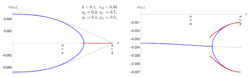
Figure 1: The dispersion relation of the Alfven modes. The original solution (blue-solid curves) in Eq. (29) is compared with the small-$k$ and small-cosine expansions in Eq. (33). The parameters are fixed as indicated in the legend for illustration.

4.2 Magneto-sonic modes from analytic algorithm

In the previous subsection, we investigated the Alfven modes encoded in the matrix equation (22a). The analytic solutions for the other matrix equation (22b) have not been know to the best of our knowledge, except for the solutions at the particular momentum directions, i.e., $k_{\parallel}=0$ or $k_{\perp}=0$ Grozdanov:2016tdf ; Hernandez:2017mch ; Armas:2022wvb . It is challenging to obtain analytic solutions including the higher-order corrections in $k$. If one invokes brute-force efforts, one has to find general solutions for a quartic equation in $\omega$, which is possible but is not an efficient path to reach compact forms of solutions. Moreover, the solutions at $k_{\parallel}=0$ suffer from the issue of the small $k$ expansion discussed in the previous subsection, giving rise to different solutions in this limit than those obtained in Refs. Grozdanov:2016tdf ; Armas:2022wvb . As in the Alfven modes, we investigate the behavior near this limit carefully.

First, we provide a simple method for the solution search that works on an order-by-order basis in $k$. This method serves as a general algorithm that can be applied to general sets of hydrodynamic equations and any other equations based on derivative expansions (see Ref. FHH for further applications), while we here focus on the quartic secular equation in $\omega$ at $k^{2}$ order. We note again that the secular equations for hydrodynamic equations, and thus their solutions, are only accurate up to a given order in $k$. Thus, the order-by-order algorithm is a suitable method for the solution search.

We begin with the leading-order solutions by putting $M_{(1)}=0$. The secular equation from $M_{(0)}$ is found to be

$$\omega\Big{[}\omega^{4}-{\mathcal{V}}^{2}k^{2}\omega^{2}+v_{A}^{2}c_{s}^{2}k^{2}k_{\parallel}^{2}\Big{]}=0,$$ (34)

with ${\mathcal{V}}^{2}:=(c_{s}^{2}+v_{A}^{2})-c_{s}^{2}v_{A}^{2}\sin^{2}\theta\geq 0$. A trivial solution, $\omega=0$, originates from the redundancy mentioned below Eq. (19). We exclude this trivial solution in the following discussions. The leading-order dispersion relations are found to be

$$\omega=\pm v_{1}k,\quad\pm v_{2}k,$$ (35)

where the two distinct velocities are given as

$$v_{1,2}=\frac{1}{\sqrt{2}}\sqrt{{\mathcal{V}}^{2}\pm\sqrt{{\mathcal{V}}^{4}-4v_{A}^{2}c_{s}^{2}\cos^{2}\theta}}\ ,$$ (36)

where the upper and lower signs are for $v_{1}$ and $v_{2}$, respectively. These modes are two pairs of counter-propagating waves called the fast and slow magneto-sonic waves. When $\theta=0$, one of the pairs reduces to the Alfven waves (29) as required by the rotational symmetry and the other pair reduces to the sound modes without modification of the sound velocity because of the absence of a magnetic pressure according to the Gauss law $\delta B_{z}=-k_{\perp}\delta B_{x}/k_{\parallel}=0$. In this limit, one finds that $\{v_{1},v_{2}\}=\{c_{s},v_{A}\}$ when $c_{s}\geq v_{A}$ and $\{v_{1},v_{2}\}=\{v_{A},c_{s}\}$ when $c_{s}<v_{A}$.

It is important to note that a pair of counter-propagating waves acquires the same dissipative corrections at $k^{2}$ order in the absence of parity-breaking effects. Therefore, the general solutions should be found in the forms

$$\omega=\pm v_{1}k-iw_{1}k^{2},\quad\omega=\pm v_{2}k-iw_{2}k^{2},$$ (37)

where $w_{1,2}$ are independent of $k$ and are determined below. Accordingly, one can make an ansatz for the factorized form of the quartic secular equation as

$$f_{\rm ans}(\omega) = \{\omega-(v_{1}k-iw_{1}k^{2})\}\{\omega-(-v_{1}k-iw_{1}k^{2})\}$$ (38)

$$\times\{\omega-(v_{2}k-iw_{2}k^{2})\}\{\omega-(-v_{2}k-iw_{2}k^{2})\}$$

$$+{\mathcal{O}}(\omega^{3}k^{3})+{\mathcal{O}}(\omega^{2}k^{4})+{\mathcal{O}}(\omega^{1}k^{5})+{\mathcal{O}}(\omega^{0}k^{6}).$$

The uncertainties at $k^{3}$ order in each solution result in the uncertainties indicated in the last line. These uncertainties are not of our interest here, since they are not improved unless the constitutive equations are improved beyond the first-order derivative expansions. The following computation is greatly simplified by identifying these irrelevant higher-order terms and getting rid of them at this stage. Expanding $f_{\rm ans}(\omega)$, we should only retain the relevant terms as

$$f_{\rm ans}(\omega)=\omega^{4}+g_{2}(k)\omega^{3}+g_{3}(k)\omega^{2}+g_{4}(k)\omega+g_{5}(k),$$ (39)

where $g_{n}$ denotes the $n$-th polynomial of $k$ stemming from the expansion of Eq. (38). As mentioned above, we should not, or do not have to, retain the terms higher than $n$ that could only be relevant beyond the first-order hydrodynamics.

The ansatz (39) is matched to the secular equation from Eq. (22b). Consistently to the above order counting, we only need to retain the terms at the same orders in $k$ in the secular equation. Then, the matching for the coefficients in the $\omega^{3}$ and $\omega^{1}$ terms lead to coupled linear equations

$$v_{2}^{2}w_{1}+v_{1}^{2}w_{2}=\frac{1}{2}W_{1},$$ (40a)

$$w_{1}+w_{2}=\frac{1}{2}W_{2},$$ (40b)

The explicit forms of $W_{1,2}$ are given as

$$W_{1} = \eta^{\prime}_{\parallel}\Big{(}c_{s}^{2}\cos^{2}(2\theta)+\frac{v_{A}^{2}\sin^{2}\theta}{1-v_{A}^{2}}\Big{)}+\rho^{\prime}_{\perp}c_{s}^{2}\frac{1-v_{A}^{2}\cos^{2}\theta}{1-v_{A}^{2}}$$ (41a)

$$+\zeta^{\prime}_{\parallel}\frac{v_{A}^{2}}{1-v_{A}^{2}}\cos^{2}\theta+\big{\{}\zeta^{\prime}_{\parallel}-2\zeta^{\prime}_{\times}+(\zeta^{\prime}_{\perp}+\eta^{\prime}_{\perp})\big{\}}c_{s}^{2}\sin^{2}\theta\cos^{2}\theta,$$

$$W_{2} = \eta^{\prime}_{\parallel}\Big{(}1+\frac{v_{A}^{2}}{1-v_{A}^{2}}\sin^{2}\theta\Big{)}+\rho^{\prime}_{\perp}\Big{(}1+\frac{v_{A}^{2}c_{s}^{2}}{1-v_{A}^{2}}\sin^{2}\theta\Big{)}$$ (41b)

$$+\frac{\zeta^{\prime}_{\parallel}}{1-v_{A}^{2}}\cos^{2}\theta+\big{(}\zeta^{\prime}_{\perp}+\eta^{\prime}_{\perp})\sin^{2}\theta,$$

where all the viscous coefficients are normalized by the enthalpy as in Eq. (27). Note that the coefficients in the $\omega^{2}$ and $\omega^{0}$ terms are automatically matched when one inserts $v_{1,2}$ in the leading-order solutions (36) because the unknowns $w_{1,2}$ are not involved. It is now a quite simple task to solve the above linear equations to find the solutions

$$w_{1}=-\frac{W_{1}-v_{1}^{2}W_{2}}{2(v_{1}^{2}-v_{2}^{2})},\quad w_{2}=+\frac{W_{1}-v_{2}^{2}W_{2}}{2(v_{1}^{2}-v_{2}^{2})}.$$ (42)

As expected in the ansatz (38), $w_{1}$ and $w_{2}$ are interchanged when we interchange $v_{1}$ and $v_{2}$. The simple algorithm leading to these analytic solutions can be applied to general equations based on derivative expansions even with higher-order terms in $\omega$ and/or $k$.

Now, making the use of the lesson from the Alfven waves discussed in Sec. 4.1, we point out that the magneto-sonic modes also suffer from the breakdown of the small $k$ expansion near $\theta=\pi/2$. This is again caused by another small quantity, $\cos\theta$, that induces divergence in the higher-order terms in the small $k$ expansion. When the cosine factor becomes small near $\theta=\pi/2$, one should use the small cosine expansion to get a correct result. To see this issue, we first take the limit $\theta\to\pi/2$ in the velocities (36). In this limit, one finds that

$$v_{1}(\theta=\frac{\pi}{2})=\sqrt{c_{s}^{2}+v_{A}^{2}-c_{s}^{2}v_{A}^{2}},\quad v_{2}(\theta=\frac{\pi}{2})=0.$$ (43)

The slow magneto-sonic waves do not propagate in the perpendicular direction and become purely diffusive modes. This implies the potential occurrence of the issue because, if there were a linear term, the counter-propagating modes should have a degenerate damping rate because of the parity invariance. The damping rates $w_{1,2}$ in the same limit read

$$w_{1}(\theta=\frac{\pi}{2}) = \frac{1}{2}\Big{(}\eta^{\prime}_{\perp}+\zeta^{\prime}_{\perp}+\rho^{\prime}_{\perp}(1-c_{s}^{2})^{2}\frac{v_{A}^{2}}{v_{1}^{2}}\Big{)},$$ (44a)

$$w_{2}(\theta=\frac{\pi}{2}) \overset{?}{=} \frac{\eta^{\prime}_{\parallel}}{2(1-v_{A}^{2})}+\frac{\rho^{\prime}_{\perp}c_{s}^{2}}{2v_{1}^{2}(1-v_{A}^{2})}.$$ (44b)

Just below, we confirm that the above degenerate $w_{2}(\theta=\frac{\pi}{2})$ is not a correct result. To get the correct result, we take the limit $\theta\to\pi/2$ in Eq. (25). Then, the matrix equation reads

$$\begin{pmatrix}-i\frac{Bc_{s}^{2}}{h(1-v_{A}^{2})}\rho^{\prime}_{\perp}k_{\perp}^{2}&-k_{\perp}B&\omega+i\rho^{\prime}_{\perp}k_{\perp}^{2}&0\\ \omega&-hk_{\perp}&h\frac{v_{A}^{2}}{B}\omega&0\\ -c_{s}^{2}k_{\perp}&h\omega+i(\zeta_{\perp}+\eta_{\perp})k_{\perp}^{2}&-h\frac{v_{A}^{2}}{B}k_{\perp}&0\\ 0&0&0&h(1-v_{A}^{2})\omega+i\eta_{\parallel}k_{\perp}^{2}\end{pmatrix}\begin{pmatrix}\delta\epsilon\\ \delta u_{x}\\ \delta B_{z}\\ \delta u_{z}\end{pmatrix}=0,$$ (45)

where we used $\delta B_{x}=-k_{\parallel}\delta B_{z}/k_{\perp}=0$ from the Gauss law (17a). Similarly to the case of the Alfven modes (31), one readily finds decoupling of a flow perturbation $\delta u_{z}$ of which the dispersion relation is solely governed by the shear viscosity $\eta_{\parallel}$. Diagonalizing the remaining three modes and retaining the terms in the $k^{2}$ order, the dispersion relations at $\theta=\pi/2$ are found to be

$$\omega_{1,2}(\theta=\frac{\pi}{2}) = \pm v_{1}k_{\perp}-\frac{i}{2}\Big{(}\eta^{\prime}_{\perp}+\zeta^{\prime}_{\perp}+\rho^{\prime}_{\perp}(1-c_{s}^{2})^{2}\frac{v_{A}^{2}}{v_{1}^{2}}\Big{)}k_{\perp}^{2}+{\mathcal{O}}(k_{\perp}^{3}),$$ (46a)

$$\omega_{3}(\theta=\frac{\pi}{2}) = -\frac{i\rho^{\prime}_{\perp}c_{s}^{2}}{v_{1}^{2}(1-v_{A}^{2})}k_{\perp}^{2}+{\mathcal{O}}(k_{\perp}^{4}),$$ (46b)

$$\omega_{4}(\theta=\frac{\pi}{2}) = -\frac{i\eta^{\prime}_{\parallel}}{1-v_{A}^{2}}k_{\perp}^{2}+{\mathcal{O}}(k_{\perp}^{4}).$$ (46c)

Here, $v_{1}=v_{1}(\theta=\pi/2)$ in Eq. (43) is understood. The fast magneto-sonic modes (46a) remain propagating modes, and still have the degenerate damping rate that agrees with $w_{1}(\theta=\pi/2)$ in Eq. (44a). In contrast, the slow magneto-sonic modes reduce to the two purely diffusive modes, and the damping rates split into two distinct ones that only depend on either $\eta^{\prime}_{\parallel}$ or $\rho^{\prime}_{\perp}$. They are different from the degenerate damping rate $w_{2}(\theta=\pi/2)$ in Eq. (44b) that was shown in Refs. Grozdanov:2016tdf ; Armas:2022wvb .

Now, we investigate the behaviors near $\theta=\pi/2$. When $\cos\theta<\hat{k}$, one should organize a series representation with respect to $\cos\theta$, as we have discussed in Sec. 33. To find the solutions in the series representations, one can apply the same algorithm introduced above. Then, we find the solutions in the form

$$\omega_{i}(\cos\theta)=\tilde{\omega}_{i}-\frac{\tilde{\omega}_{i}^{3}X_{3}+\tilde{\omega}_{i}^{2}X_{2}+\tilde{\omega}_{i}X_{1}+X_{0}}{\prod_{i\neq j}(\tilde{\omega}_{i}-\tilde{\omega}_{j})}\cos^{2}\theta+{\mathcal{O}}(\cos^{4}\theta),$$ (47)

where $\tilde{\omega}_{i}$ on the right-hand side are the solutions for Eq. (45) at $\cos^{2}\theta=0$, i.e., $\tilde{\omega}=\omega(\theta=\pi/2)$. It is interesting that the fast and slow sonic-modes, which were previously labeled as $\omega_{1,2}$ and $\omega_{3,4}$, are mixed among themselves in the correction terms of order $\cos^{2}\theta$. The explicit forms of $X_{i}$ are given as

$$X_{0} = c_{s}^{2}v_{A}^{2}k^{4}+k^{6}c_{s}^{2}\rho^{\prime}_{\perp}\Big{[}(\zeta^{\prime}_{\perp}+\eta^{\prime}_{\perp})-\frac{2\zeta^{\prime}_{\times}}{1-v_{A}^{2}}+\frac{\zeta^{\prime}_{\parallel}-2(2-v_{A}^{2})\eta^{\prime}_{\parallel}}{(1-v_{A}^{2})^{2}}\Big{]},$$ (48a)

$$X_{1} = ik^{4}\Big{[}\frac{v_{A}^{2}(\eta^{\prime}_{\parallel}-\zeta^{\prime}_{\parallel}+c_{s}^{2}\rho^{\prime}_{\perp})}{1-v_{A}^{2}}-c_{s}^{2}(\zeta^{\prime}_{\parallel}+\zeta^{\prime}_{\perp}-2\zeta^{\prime}_{\times}-4\eta^{\prime}_{\parallel}+\eta^{\prime}_{\perp})\Big{]}$$ (48b)

$$+\frac{ik^{6}}{(1-v_{A}^{2})^{2}}\rho^{\prime}_{\perp}\Big{[}c_{s}^{2}v_{A}^{2}\big{(}\zeta_{\times}^{\prime\,2}+2\zeta^{\prime}_{\times}\eta^{\prime}_{\parallel}-\zeta^{\prime}_{\parallel}(\zeta^{\prime}_{\perp}+\eta^{\prime}_{\perp})+3\eta^{\prime}_{\parallel}(\zeta^{\prime}_{\perp}+\eta^{\prime}_{\perp})\big{)}$$

$$+(1-v_{A}^{2})\big{(}\zeta_{\times}^{\prime\,2}-\zeta^{\prime}_{\parallel}(\zeta^{\prime}_{\perp}+\eta^{\prime}_{\perp})+2\eta^{\prime}_{\parallel}(\zeta^{\prime}_{\perp}+\zeta^{\prime}_{\times}+\eta^{\prime}_{\perp})\big{)}\Big{]},$$

$$X_{2} = -c_{s}^{2}v_{A}^{2}k^{2}-\frac{k^{4}}{(1-v_{A}^{2})^{2}}\Big{[}c_{s}^{2}v_{A}^{2}\rho^{\prime}_{\perp}\big{(}\zeta^{\prime}_{\parallel}-2(1-v_{A}^{2})\zeta^{\prime}_{\perp}-(1+v_{A}^{2})\eta^{\prime}_{\parallel}-2(1-v_{A}^{2})\eta^{\prime}_{\perp}\big{)}$$ (48c)

$$-(1-v_{A}^{2})\Big{\{}\rho^{\prime}_{\perp}\big{(}\,v_{A}^{2}\eta^{\prime}_{\parallel}+(1-v_{A}^{2})(\zeta^{\prime}_{\perp}+\eta^{\prime}_{\perp})\,\big{)}$$

$$+\zeta_{\times}^{\prime\,2}+2\eta^{\prime}_{\parallel}(\zeta^{\prime}_{\perp}+\zeta^{\prime}_{\times}+\eta^{\prime}_{\perp})-\zeta^{\prime}_{\parallel}(\zeta^{\prime}_{\perp}+\eta^{\prime}_{\perp}+\rho^{\prime}_{\perp})\Big{\}}\Big{]},$$

$$X_{3} = \frac{ik^{2}}{1-v_{A}^{2}}\Big{[}\zeta^{\prime}_{\parallel}-(1-v_{A}^{2})(\zeta^{\prime}_{\perp}+\eta^{\prime}_{\perp})-v_{A}^{2}(\eta^{\prime}_{\parallel}+c_{s}^{2}\rho^{\prime}_{\perp})\Big{]},$$ (48d)

These results should replace the naive small $k$ expansion when $\cos\theta<\hat{k}$.

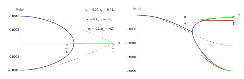
Figure 2: The dispersion relation for the slow magneto-sonic modes. Blue curves show the “exact solution” obtained by Mathematica. Dotted curves show the small-$k$ expansion in Eq. (42). Red and green curves show the small-cosine expansion (47), instead. In the red curve, we further expand the series coefficients up to $k^{2}$.

In Fig. 2, we show the dispersion relations for the slow magneto-sonic modes. The “exact solution” for Eq. (22b) is shown by blue-solid curves, of which the analytic forms are obtained by an automated command in Mathematica; The complicated expressions are not useful to be shown here. Note that the “exact solution” contains the higher-order corrections beyond the $k^{2}$ order and does not mean that it is the true goal for the first-order hydrodynamics. As the angle approaches the right angle $\theta=\pi/2$, the small $k$ expansion, shown by dotted curves, deviates from the “exact solution” even at a fixed small value of $k$. Instead of the small $k$ expansion, the small-cosine expansion (47) should be effective in this region as discussed above. The green curves show the small-cosine expansion (47) without an expansion for the momentum $k$, while the red curves show the same expansion but with a further expansion of the series coefficients up to $k^{2}$. Both curves well reproduce the branching in the imaginary part near the right angle. At $\theta=\pi/2$, i.e., $\cos\theta=0$, the deviation between the green and red curves solely comes from the choice of $\tilde{\omega}_{i}$ with or without the higher-order terms in $k$ in Eq. (47). When $\cos\theta\not=0$, the coefficients for the $\cos^{2}\theta$ corrections also contain the $k$ dependence in $X_{i}$ as well as $\tilde{\omega}_{i}$ both in the numerator and denominator.

Next, we comment on extracting magnitudes of the transport coefficients by comparing the linear-mode solutions with experiments/observations. Remarkably, the general solution obtained in Eq. (42) is necessary to determine the cross bulk viscosity $\zeta_{\times}$, which cannot be determined with the limiting solutions at $\theta=0,\pi/2$ Grozdanov:2016tdf . It is a cross quantity between the parallel and perpendicular directions with respect to the magnetic field, and cannot be induced along a single direction at $\theta\not=0$ or $\pi/2$ (see Eqs. (44) and (49) below). Yet, even with the complete solution, one cannot determine a separation between $\eta^{\prime}_{\perp}$ and $\zeta^{\prime}_{\perp}$ that appears only in the sum in Eq. (25b) and the general solutions (41) accordingly. In the Alfven modes (29), $\eta^{\prime}_{\perp}$ and $\rho^{\prime}_{\parallel}$ also appear in the sum in the small $k$ expansion. However, the dependence on these two transport coefficients is split in Eq. (30) at $\theta=\pi/2$, and they can be determined with the linear-mode solutions. The other pair $\eta^{\prime}_{\perp}$ and $\rho^{\prime}_{\parallel}$ appear separately in the magneto-sonic modes in Eq. (46).

Before closing this section, it is also instructive to confirm the limit of $\theta\to 0,\pi$, i.e., $k_{\perp}\to 0$. As mentioned below Eq. (36), one of the pairs should become degenerate with the Alfven modes because of the rotational symmetry. When $\theta=0$, we have

$$W_{1}(\theta=0) = \eta^{\prime}_{\parallel}c_{s}^{2}+\rho^{\prime}_{\perp}c_{s}^{2}+\zeta^{\prime}_{\parallel}\frac{v_{A}^{2}}{1-v_{A}^{2}},$$ (49a)

$$W_{2}(\theta=0) = \eta^{\prime}_{\parallel}+\rho^{\prime}_{\perp}+\frac{\zeta^{\prime}_{\parallel}}{1-v_{A}^{2}}.$$ (49b)

Then, we find that, when $c_{s}\geq v_{A}$,

$$w_{1}(\theta=0)=\frac{\zeta^{\prime}_{\parallel}}{2(1-v_{A}^{2})},\quad w_{2}(\theta=0)=\frac{1}{2}(\eta^{\prime}_{\parallel}+\rho^{\prime}_{\perp}),$$ (50)

and that, when $c_{s}<v_{A}$,

$$w_{1}(\theta=0)=\frac{1}{2}(\eta^{\prime}_{\parallel}+\rho^{\prime}_{\perp}),\quad w_{2}(\theta=0)=\frac{\zeta^{\prime}_{\parallel}}{2(1-v_{A}^{2})}.$$ (51)

In both cases, either of the pairs becomes degenerate with the Alfven modes (29). The other pair is the sound modes damped by the bulk viscosity. The shear viscosity does not contribute to the damping rate in this limit, differently from the usual sound modes in the absence of a magnetic field.

5 Causality and stability

In the last section, we have obtained the pairs of the Alfven waves (29) and the slow and fast magneto-sonic waves (37). In this section, we show that the phase velocities of the Alfven and magneto-sonic waves are always smaller than the speed of light and that the first-order derivative corrections in those solutions (29) and (37) always act as damping factors as long as the transport coefficients satisfy the inequalities (11) required by the second law of thermodynamics. The former implies causality in the ideal MHD. The latter implies a stability of equilibrium state in the fluid rest frame where the linear-mode analysis has been performed in the last section.

However, the above two properties in general do not guarantee causality beyond the ideal order or stability in an arbitrary Lorentz frame. We briefly discuss causality and stability of relativistic MHD along with the recent developments in the literature.

5.1 The Alfven and magneto-sonic velocities in the ideal MHD

First, we focus on the linear terms in $k$, putting the higher-order terms aside. This is the ideal MHD limit. We assume that the sound velocity satisfies an inequality

$$0\leq c_{s}\leq 1.$$ (52)

We also assume that the Alfven velocity (24) satisfies an inequality

$$0\leq v_{A}\leq 1.$$ (53)

The latter inequality is evident when the energy density and pressure are separated as in Eq. (13), where the Alfven velocity reads $v_{A}^{2}=\frac{B^{2}/\mu_{m}}{\epsilon+P+B^{2}/\mu_{m}}$. This inequality should hold unless a strong coupling between the matter and magnetic components significantly reduces the total energy density and pressure.

Under the above inequalities, one can show that the velocities of the magneto-sonic waves (36) satisfy the inequalities

$$0\leq v_{2}\leq c_{s}\leq v_{1}\leq 1\quad{\rm and}\quad 0\leq v_{2}\leq v_{A}\leq v_{1}\leq 1.$$ (54)

Here, the relative magnitude between $c_{s}$ and $v_{A}$ is not assumed. A straightforward proof is given in Appendix A.1. The inequalities in Eqs. (53) and (54) indicate that the Alfven and magneto-sonic waves propagate with subluminal speeds in the ideal MHD.

5.2 Dissipative nature of the first-order corrections in the fluid rest frame

Next, we focus on the $k^{2}$ terms in the dispersion relations. Since all the present transport coefficients are dissipative in nature, the Alfven and magneto-sonic waves are expected to acquire damping effects. We show that the pure imaginary $k^{2}$ terms, which have been found in the previous section, take definite signs as long as the transport coefficients satisfy the inequalities (11) required by the second law of thermodynamics.

In the Alfven waves (29), it is clear that the pure imaginary coefficient in front of $k^{2}$ is always negative for $\eta_{\parallel,\perp}\geq 0$ and $\rho_{\parallel,\perp}\geq 0$ required by the inequalities (11).

The magneto-sonic waves also have the pure imaginary corrections at the $k^{2}$ order. The explicit forms of $w_{1,2}$ in Eq. (42) are given as

$$w_{1,2}(\theta) = \frac{\mp 1}{2(v_{1}^{2}-v_{2}^{2})}\Big{[}\,\eta^{\prime}_{\parallel}\Big{(}c_{s}^{2}\cos^{2}(2\theta)-v_{1,2}^{2}+\frac{(1-v_{1,2}^{2})v_{A}^{2}}{1-v_{A}^{2}}\sin^{2}\theta\Big{)}$$ (55)

$$+\rho^{\prime}_{\perp}\Big{(}c_{s}^{2}-v_{1,2}^{2}+\frac{(1-v_{1,2}^{2})v_{A}^{2}c_{s}^{2}}{1-v_{A}^{2}}\sin^{2}\theta\Big{)}+(\eta^{\prime}_{\perp}+\zeta^{\prime}_{\perp})(c_{s}^{2}\cos^{2}\theta-v_{1,2}^{2})\sin^{2}\theta$$

$$+\zeta^{\prime}_{\parallel}\frac{{\mathcal{V}}^{2}-v_{1,2}^{2}-c_{s}^{2}\cos^{2}\theta}{1-v_{A}^{2}}\cos^{2}\theta-2\zeta^{\prime}_{\times}c_{s}^{2}\cos^{2}\theta\sin^{2}\theta\,\Big{]},$$

where the upper and lower signs are for $w_{1}$ and $w_{2}$, respectively. As detailed in Appendix A.2, one can show that

$$w_{1,2}(\theta)\geq 0,$$ (56)

for any angle $\theta$. This means that the pure imaginary corrections always take negative signs [see the conventions in Eq. (37).] We note that the semi-positivity of $w_{1,2}$ can be shown irrespective of the sign of $\zeta^{\prime}_{\times}$ as long as the transport coefficients satisfy the inequalities (11), none of which indeed specifies the sign of $\zeta^{\prime}_{\times}$.

When the angle approaches $\theta=\pi/2$, one should refer to the small-cosine expansions in Eqs. (33) and (46) or (47). The leading-order terms of order $\cos^{0}\theta$, i.e., when $\theta=\pi/2$, indicate purely diffusive modes with definite signs. The cosine corrections are expected to be smaller than these leading-order terms within the regions of validity for the cosine expansions. Then, the signs should remain definite as seen in Figs. 1 and 2 with the corrections.

The above inequalities imply that both the Alfven and magneto-sonic waves are damped out by exponential factors for an observer in the fluid rest frame where the linear-mode analysis has been performed. However, those inequalities are not sufficient conditions for stability in an arbitrary Lorentz frame, but are necessary conditions. We discuss stability and causality conditions in a more general perspective below.

5.3 Covariant stability in anisotropic systems

It has been known that diffusive modes in the first-order hydrodynamics are acausal and that such diffusive modes, which are damped out in the fluid rest frame, can be transformed into growing modes in a general Lorentz frame Hiscock:1985zz . Relativistic hydrodynamic theories containing such instability may not work in practice because the stability of local equilibria in a certain reference frame, e.g., a lab frame as often interested, is not guaranteed. Therefore, it is important to understand the origin of the instability and the necessary and/or sufficient conditions for the covariant stability where the local equilibria are stable in any Lorentz frame.

Here, we briefly discuss the covariant stability for MHD with a slight extension of the recent discussions by Gavassino for isotropic systems Gavassino:2021owo ; Gavassino:2023myj . We write the solutions for the linear perturbations (21) in a covariant form

$$\Psi=\tilde{\Psi}e^{-ik_{\mu}x^{\mu}},$$ (57)

where $\Psi$ is an eigenvector and the corresponding momentum $k^{\mu}=(\omega,{\bm{k}})$ satisfies a dispersion relation obtained from the (linearized) hydrodynamic equations. However, as we have seen in the previous sections, the dispersion relations are not given in Lorentz-invariant forms like the free-particle on-shell conditions in quantum field theories, which is due to the derivative expansion. Therefore, we need to understand how the dispersion relations are transformed by a Lorentz boost.

First, notice that, in dissipative hydrodynamics, the spatial component of the momentum ${\bm{k}}$ develops an imaginary part in a general Lorentz frame due to the mixing between $\omega$ and ${\bm{k}}$ under Lorentz boosts. For the general solution (57) to be covariantly stable, one should have $\Im m\,[k_{\mu}x^{\mu}]\leq 0$. For this condition to be satisfied for observers in the forward light cone, the imaginary part of $k^{\mu}$ should be a vector lying outside the forward light cone, requiring that

$$\Im m\,\omega\leq-|\Im m\,{\bm{k}}|\quad{\rm or}\quad(\Im m\,k^{\mu})(\Im m\,k_{\mu})=-(\Im m\,\omega)^{2}+|\Im m\,{\bm{k}}|^{2}\geq 0.$$ (58)

Combining the above inequalities, one finds a necessary condition for the covariant stability

$$\Im m\,\omega\leq|\Im m\,{\bm{k}}|\,.$$ (59)

This is an extension of the condition for an isotropic system obtained by Heller et al. from the analytic property of a general retarded propagator in causal quantum field theory theories Heller:2022ejw and interpreted by Gavassini as the covariantly stability condition for relativistic dissipative hydrodynamics Gavassino:2023myj . The inequality (59) is a stronger condition than that for isotropic systems where there is essentially only one independent component of ${\bm{k}}$. For MHD, two of the three components should be treated independently as there remains a rotational symmetry around the magnetic-field direction.

When there are dissipative effects, i.e., $\Im m\,\omega\not=0$, with $\Im m\,{\bm{k}}=0$ in the fluid rest frame, one may consider successive multiple Lorentz boosts; The first boost generates an imaginary part of ${\bm{k}}$ due to the mixing with $\omega$, and the subsequent boosts require the inequality (59) for the causal stability. The result of these successive boosts is not equivalent to that of a single boost by a sum of the boost velocities, because of the non-Abelian nature of the Lorentz group. In analogy with the discussion about the Thomas precession jackson1999classical , such a sequence of Lorentz boosts is required to move from one Lorentz frame to another, e.g., from the rest frame of a fluid cell to the lab frame, when the fluid cell is accelerated.

It is instructive to explicitly see the occurrence of instability when the inequality (59) is not satisfied Gavassino:2023myj . In fact, the dispersion relations turn into unstable ones when boosted by a velocity

$${\bm{v}}=\frac{\Im m\,{\bm{k}}}{\Im m\,\omega}\,,$$ (60)

that satisfies $|{\bm{v}}|\leq 1$ when the inequality (59) is not satisfied. Boosting the imaginary part of the momentum, one finds that

$$\Im m\,k^{\mu}\to\Im m\,k^{\prime\mu} = \gamma(\Im m\,\omega-{\bm{v}}\cdot\Im m\,{\bm{k}},-\gamma{\bm{v}}\Im m\,\omega+\Im m\,{\bm{k}}+\frac{(\gamma-1){\bm{v}}\cdot\Im m\,{\bm{k}}}{v^{2}}{\bm{v}})$$ (61)

$$= \gamma(\frac{(\Im m\,\omega)^{2}-|\Im m\,{\bm{k}}|^{2}}{\Im m\,\omega},{\bm{0}})\,.$$

This means that an observer in the new frame claims the existence of an unstable Fourier mode because $\Im m\,\omega^{\prime}>0$ and $\Im m\,{\bm{k}}^{\prime}=0$. Therefore, the inequality (59) is indeed necessary for the covariant stability.

If the inequality (59) is satisfied in one of the Lorentz frames, it is, by construction, satisfied in all the Lorentz frames connected by Lorentz boosts. Then, the covariant stability will be fulfilled if signals only reach observers inside the forward light cone, i.e., if theories respect causality (see a theorem in Sec. III.B in Ref. Gavassino:2021kjm ). However, it has been known that, in dissipative hydrodynamics, signals reach observers outside the forward light cone. The acausal tails of dissipative modes are not only illegitimate in relativity in the first place but also observed as unstable modes outside the light cone (see a theorem in Sec. III.A in Ref. Gavassino:2021kjm ). This is because, for a spacelike separation $(y-x)^{2}>0$, there is a Lorentz boost that inverts the chronicle ordering as $y^{0}-x^{0}\to y^{\prime\,0}-x^{\prime\,0}=-(y^{0}-x^{0})$, making the meaning of dissipation and growth observer-dependent concepts. Therefore, the covariant stability is fulfilled only in causal theories. The first-order MHD is stable in the fluid rest frame as shown above, but is not causal. The subluminal magneto-sonic velocities (54) only serve as necessary conditions for causality once the dissipative effects are included.

Causality is often a consequence of subtle cancellation among the acausal tails leaking across the light cone. A well-known example is the Klein-Gordon field in quantum field theory Peskin:1995ev . In Ref. Gavassino:2023mad , it is stated that any dispersion relation can leak across the light cone unless a medium is not dispersive or, in other words, dispersion relations are polynomials of the first order at most, i.e., $\omega(k)=a_{0}+a_{1}k$ (see also Ref. Heller:2022ejw ). This implies that inspecting each dispersion relation alone does not guarantee causality. Notions of velocities for a single dispersion relation, such as the front velocity, the group velocity, and the phase velocity, may be useful for screening apparently acausal theories, but do not serve as a sufficient causality test; Besides, it should be noticed that the font velocity is defined at the ultraviolet limit $k\to\infty$ outside the hydrodynamic regime. Instead, it will be useful to investigate causal structures of a set of partial differential equations with the method of characteristics (see, e.g., Refs. Izumi:2014loa ; Bemfica:2017wps and references therein), though it will require more efforts in future works. It is worth adding that the covariantly stable condition (59) is derived independently of any notion of velocities (see also Theorem 2 in Ref. Gavassino:2023myj where a criterion of causality is manifestly implemented without any notion of velocities).

6 Conclusion and outlook

In this paper, we investigated linear waves in relativistic magnetohydrodynamics in detail. Especially, in Sec. 4.2, we provided a simple and general analytic algorithm for the solution search. Based on this algorithm, we showed analytic solutions for the magneto-sonic waves that have been missing in the literature for a long time. The algorithm can be applied to other hydrodynamic equations or any general set of equations based on a derivative expansion. We will provide an application elsewhere FHH . Also, while we focused on the Landau frame in the present work, it is interesting to investigate analytic solutions in a general choice of hydrodynamic variables (cf. Ref. Armas:2022wvb ).

On the other hand, we also found that the small-momentum expansion for the solutions breaks down in MHD when the momentum direction is nearly or exactly perpendicular to an equilibrium magnetic field. This issue occurs both in the Alfven and magneto-sonic waves and stems from the competition between two small quantities involved in the solutions that are the momentum and the trigonometric functions representing the spatial anisotropy in MHD, i.e., a cosine function in the present convention. When the cosine becomes small near the right angle, we found that the higher-order terms in the small-momentum expansion diverge, spoiling the small-momentum expansion. The breakdown of the small-momentum expansion can be a general issue emerging in anisotropic systems. We provided alternative expressions of the solutions based on the small-cosine expansion in Eqs. (33) and (47) that work accurately near the right angle as shown in Figs. 1 and 2.

Lastly, we investigated the issues of causality and stability in the first-order relativistic MHD based on the analytic solutions. We showed that the Alfven and magneto-sonic velocities are less than the speed of light and that the first-order corrections always act as damping effects in the fluid rest frame. As mentioned in Sec. 5.3, these conditions are, however, not sufficient for the covariant stability, i.e., the stability in all the Lorentz frames. The main and general reason is that dissipative hydrodynamics exhibits acausal propagation across the forward light cone. Such acausal signals can be observed as unstable modes in the spacelike regions, indicating an imtimate connection between the issues of causality and stability. So far, the method of moment expansion, which leads to the Israel-Stewart theory, has been invoked in Refs. Denicol:2018rbw ; Denicol:2019iyh to formulate causal and stable MHD (see also Ref. Hattori:2022hyo for a review). It is yet left as an open question to formulate covariantly stable MHD based on the magnetic-flux conservation (cf. Sec. 2). Other future works include computation of the transport coefficients (see Hattori:2016cnt ; Hattori:2016lqx ; Hattori:2017qih ; Li:2017tgi ; Fukushima:2017lvb ; Kurian:2018dbn ; Li:2018ufq ; Fukushima:2019ugr ; Astrakhantsev:2019zkr ; Fukushima:2021got ; Peng:2023rjj for recent studies). These developments will promote further numerical studies Inghirami:2016iru ; Inghirami:2019mkc ; Nakamura:2022idq ; Nakamura:2022wqr ; Nakamura:2022ssn .

Appendix A inequalities

A.1 Inequalities for the Alfven and magneto-sonic velocities

We assume that the equations of state satisfy the inequalities $0\leq c_{s}\leq 1$ and $0\leq v_{A}\leq 1$ as stated in Eqs. (52) and (53). Then, we show that the velocities of the magneto-sonic waves (36) satisfy the inequalities (54), i.e.,

$$0\leq v_{2}\leq c_{s}\leq v_{1}\leq 1\quad{\rm and}\quad 0\leq v_{2}\leq v_{A}\leq v_{1}\leq 1.$$ (62)

Here, the relative magnitude between $c_{s}$ and $v_{A}$ is not assumed.

It is easy to show that ${\mathcal{V}}^{2}\geq 0$ by comparing the magnitudes of the two terms in ${\mathcal{V}}^{2}$ as

$$(c_{s}^{2}+v_{A}^{2})^{2}-(c_{s}^{2}v_{A}^{2}\sin^{2}\theta)^{2}=c_{s}^{4}+v_{A}^{4}+c_{s}^{2}v_{A}^{2}(2-c_{s}^{2}v_{A}^{2}\sin^{4}\theta)\geq 0.$$ (63)

Then, it is obvious that $v_{1,2}\geq 0$.

Next, we show that $v_{1,2}\leq 1$. Comparing the two sides, one finds that

$$(2-{\mathcal{V}}^{2})^{2}-\sqrt{{\mathcal{V}}^{4}-4v_{A}^{2}c_{s}^{2}\cos^{2}\theta}^{\,2} = -4(1-v_{A}^{2})(1-c_{s}^{2})\leq 0.$$ (64)

Note also that $2-{\mathcal{V}}^{2}=(2-c_{s}^{2}-v_{A}^{2})+c_{s}^{2}v_{A}^{2}\sin^{2}\theta\geq 0$. Then, one can conclude that $v_{1,2}\leq 1$.

Lastly, we show the relative magnitudes of $v_{1,2}$ to $c_{s}$ and $v_{A}$. The difference between $v_{1,2}$ and $c_{s}$ reads

$$c_{s}^{2}-v_{1,2}^{2} = (c_{s}^{2}-\frac{1}{2}{\mathcal{V}}^{2})\mp\frac{1}{2}\sqrt{{\mathcal{V}}^{4}-4v_{A}^{2}c_{s}^{2}\cos^{2}\theta}.$$ (65)

The relative magnitudes of the two terms is examined as

$$\frac{1}{2^{2}}\big{(}{\mathcal{V}}^{4}-4v_{A}^{2}c_{s}^{2}\cos^{2}\theta\big{)}-(c_{s}^{2}-\frac{1}{2}{\mathcal{V}}^{2})^{2} = (-v_{A}^{2}\cos^{2}\theta-c_{s}^{2}+{\mathcal{V}}^{2})c_{s}^{2}$$ (66)

$$= (1-c_{s}^{2})v_{A}^{2}c_{s}^{2}\sin^{2}\theta$$

$$\geq 0.$$

Therefore, the sign of the difference in Eq. (65) is determined by that of the square-root term regardless of the sign of the other term. Then, one can conclude that $v_{2}\leq c_{s}\leq v_{1}$. By the same token, one can examine the difference

$$v_{A}^{2}-v_{1,2}^{2} = (v_{A}^{2}-\frac{1}{2}{\mathcal{V}}^{2})\mp\frac{1}{2}\sqrt{{\mathcal{V}}^{4}-4v_{A}^{2}c_{s}^{2}\cos^{2}\theta}.$$ (67)

The relative magnitudes of the two terms is examined as

$$\frac{1}{2^{2}}\big{(}{\mathcal{V}}^{4}-4v_{A}^{2}c_{s}^{2}\cos^{2}\theta\big{)}-(v_{A}^{2}-\frac{1}{2}{\mathcal{V}}^{2})^{2} = (-c_{s}^{2}\cos^{2}\theta-v_{A}^{2}+{\mathcal{V}}^{2})v_{A}^{2}$$ (68)

$$= (1-v_{A}^{2})v_{A}^{2}c_{s}^{2}\sin^{2}\theta$$

$$\geq 0.$$

Then, one can conclude that $v_{2}\leq v_{A}\leq v_{1}$.

Following the above proof, we conclude the inequalities (54).

A.2 Dissipative corrections in the fluid rest frame

The next-to-leading order solutions in the magneto-sonic modes (37) are obtained with $w_{1,2}$ given in Eq. (55). Here, we show that $w_{1,2}\geq 0$ for the transport coefficients that satisfy the inequalities (11) required by the second law of thermodynamics. In the following discussion, one can forget about the positive overall factor like $1/(2(v_{1}^{2}-v_{2}^{2}))$ that is irrelevant for examining the signs of $w_{1,2}$.

We begin with the terms associated with the bulk viscosities $\zeta_{\parallel,\perp,\times}$. Picking up these terms from $w_{1,2}$ in Eq. (55), we have

$$w^{\zeta}_{1,2}:=s_{1,2}\zeta_{\perp}+t_{1,2}\zeta_{\parallel}+u\zeta_{\times}\,,$$ (69)

where

$$s_{1,2}=\mp(c_{s}^{2}\cos^{2}\theta-v_{1,2}^{2})\sin^{2}\theta,\quad t_{1,2}=\mp\frac{{\mathcal{V}}^{2}-v_{1,2}^{2}-c_{s}^{2}\cos^{2}\theta}{1-v_{A}^{2}}\cos^{2}\theta,$$

$$u=\pm 2c_{s}^{2}\cos^{2}\theta\sin^{2}\theta.$$ (70)

One can show that $s_{1,2}\geq 0$ and $t_{1,2}\geq 0$ as we will see later. Assuming these positivities for the moment, one finds that

$$w^{\zeta}_{1,2}\geq 2\sqrt{s_{1,2}t_{1,2}\zeta_{\parallel}\zeta_{\perp}}+u\zeta_{\times}\,.$$ (71)

Further examining the relative magnitude of the two terms on the right-hand side, we have

$$4s_{1,2}t_{1,2}\zeta_{\parallel}\zeta_{\perp}-(u\zeta_{\times})^{2}\geq(4s_{1,2}t_{1,2}-u^{2})\zeta_{\times}^{2}=0\,,$$ (72)

where we used the inequality from the thermodynamic constraint (11) and the explicit forms of $s,t,u$ that, in both cases, lead to $(4s_{1,2}t_{1,2}-u^{2})=0$. Therefore, one can conclude that $w_{1,2}^{\zeta}\geq 0$ as long as $s_{1,2},t_{1,2}\geq 0$ irrespective of the sign of $u$.

To show that $s_{1,2}\geq 0$, one can arrange it with the explicit forms of $v_{1,2}^{2}$ as

$$s_{1,2} = \mp\big{(}c_{s}^{2}\cos^{2}\theta-\frac{1}{2}{\mathcal{V}}^{2}\big{)}+\frac{1}{2}\sqrt{{\mathcal{V}}^{4}-4v_{A}^{2}c_{s}^{2}\cos^{2}\theta}.$$ (73)

As for $t_{1,2}\geq 0$, one can focus on the numerator

$$(1-v_{A}^{2})t_{1,2} = \mp({\mathcal{V}}^{2}-v_{1,2}^{2}-c_{s}^{2}\cos^{2}\theta)$$ (74)

$$= \pm\big{(}c_{s}^{2}\cos^{2}\theta-\frac{1}{2}{\mathcal{V}}^{2}\big{)}+\frac{1}{2}\sqrt{{\mathcal{V}}^{4}-4v_{A}^{2}c_{s}^{2}\cos^{2}\theta}.$$

In both cases, one can show that the square-root term is always larger than the absolute value of the first term, that is,

$$\frac{1}{2^{2}}({\mathcal{V}}^{4}-4v_{A}^{2}c_{s}^{2}\cos^{2}\theta)-(c_{s}^{2}\cos^{2}\theta-\frac{1}{2}{\mathcal{V}}^{2})^{2} = -c_{s}^{2}\cos^{2}\theta(v_{A}^{2}+c_{s}^{2}\cos^{2}\theta-{\mathcal{V}}^{2})$$ (75)

$$= c_{s}^{4}\sin^{2}\theta\cos^{2}\theta(1-v_{A}^{2})$$

$$\geq 0.$$

Therefore, we have shown that $s_{1,2}\geq 0$ and $t_{1,2}\geq 0$, and accordingly that $w_{1,2}^{\zeta}\geq 0$.

We have three remaining terms associated with $\eta^{\prime}_{\parallel},\rho^{\prime}_{\perp},\eta^{\prime}_{\perp}$. The last one $\eta^{\prime}_{\perp}$ only appears with $\zeta^{\prime}_{\perp}$ in Eq. (55), so that we have already shown the positivity of this term just above. We examine the remaining two terms below. The coefficients in front of $\rho^{\prime}_{\perp}$ is arranged as

$$\frac{\mp 1}{1-v_{A}^{2}}\big{[}\,(1-v_{A}^{2})(c_{s}^{2}-v_{1,2}^{2})+(1-v_{1,2}^{2})v_{A}^{2}c_{s}^{2}\sin^{2}\theta\,\big{]}.$$ (76)

According to the inequalities (62) for the velocities, the right-hand side is semi-positive definite for $v_{2}$. As for $v_{1}$, one can arrange the expression between the square brackets as

$$(1-v_{A}^{2})(c_{s}^{2}-v_{1}^{2})-(1-v_{1}^{2})v_{A}^{2}c_{s}^{2}\sin^{2}\theta$$ (77)

$$= c_{s}^{2}(1-v_{A}^{2}+v_{A}^{2}\sin^{2}\theta)-v_{1}^{2}J$$

$$= \big{[}c_{s}^{2}(1-v_{A}^{2}+v_{A}^{2}\sin^{2}\theta)-\frac{1}{2}{\mathcal{V}}^{2}J\big{]}-\frac{J}{2}\sqrt{{\mathcal{V}}^{4}-4v_{A}^{2}c_{s}^{2}\cos^{2}\theta},$$

where $J=1-v_{A}^{2}+v_{A}^{2}c_{s}^{2}\sin^{2}\theta$. Comparing the magnitudes of the two terms, one finds that

$$\Big{[}\,\frac{J}{2}\sqrt{{\mathcal{V}}^{4}-4v_{A}^{2}c_{s}^{2}\cos^{2}\theta}\,\Big{]}^{2}-\big{[}c_{s}^{2}(1-v_{A}^{2}+v_{A}^{2}\sin^{2}\theta)-\frac{1}{2}{\mathcal{V}}^{2}J\big{]}^{2} = v_{A}^{2}c_{s}^{2}(1-v_{A}^{2})(1-c_{s}^{2})^{2}\sin^{2}\theta$$ (78)

$$\geq 0\,.$$

This means that the sign of the left-hand side in Eq. (77) is determined by that of the square-root term, which is negative. Therefore, for both $w_{1,2}$, one can conclude that the coefficients in front of $\rho_{\perp}^{\prime}$ are semi-positive definite in Eq. (76).

Lastly, the coefficients in front of $\eta^{\prime}_{\parallel}$ in Eq. (55) can be arranged as

$$\frac{\pm 1}{1-v_{A}^{2}}\big{[}(1-v_{A}^{2}\cos^{2}\theta)v_{1,2}^{2}-\{(1-v_{A}^{2})c_{s}^{2}\cos^{2}(2\theta)+v_{A}^{2}\sin^{2}\theta\}\big{]}.$$ (79)

Inserting the explicit forms of $v_{1,2}$, we have

$$(1-v_{A}^{2}\cos^{2}\theta)v_{1,2}^{2}-\{(1-v_{A}^{2})c_{s}^{2}\cos^{2}(2\theta)+v_{A}^{2}\sin^{2}\theta\}=K_{1,2}+L.$$ (80)

where

$$K_{1,2} = \pm\frac{1}{2}(1-v_{A}^{2}\cos^{2}\theta)\sqrt{{\mathcal{V}}^{4}-4v_{A}^{2}c_{s}^{2}\cos^{2}\theta},$$ (81a)

$$L = \frac{1}{2}(1-v_{A}^{2}\cos^{2}\theta){\mathcal{V}}^{2}-(1-v_{A}^{2})c_{s}^{2}\cos^{2}(2\theta)-v_{A}^{2}\sin^{2}\theta,$$ (81b)

where the upper and lower signs from $v_{1,2}$ are for $K_{1}$ and $K_{2}$, respectively. Examining the relative magnitude of the two terms, one finds that

$$K_{1,2}^{2}-L^{2} = \frac{1}{4}(1-v_{A}^{2})\sin^{2}(2\theta)\big{\{}v_{A}^{2}-c_{s}^{2}(2-v_{A}^{2})\cos(2\theta)\big{\}}^{2}\geq 0.$$ (82)

This inequality, together with $(1-v_{A}^{2}\cos^{2}\theta)\geq 0$, means that the overall signs in Eq. (80) are determined by that of $K_{1,2}$. Then, one can conclude that the coefficients in front of $\eta^{\prime}_{\parallel}$ are semi-positive definite for both $w_{1,2}$.

From the above, we conclude that the magneto-sonic modes (37) are damped out by the semi-positive damping factor $w_{1,2}$ given in Eq. (55). We emphasize that the semi-positivity of $w_{1,2}$ has been shown irrespective of the sign of $\zeta^{\prime}_{\times}$ as long as the transport coefficients satisfy the inequalities (11), none of which specifies the sign of $\zeta^{\prime}_{\times}$.

References

- (1) G. Inghirami, L. Del Zanna, A. Beraudo, M. H. Moghaddam, F. Becattini and M. Bleicher, Numerical magneto-hydrodynamics for relativistic nuclear collisions, Eur. Phys. J. C 76 (2016) 659 [1609.03042].
- (2) G. Inghirami, M. Mace, Y. Hirono, L. Del Zanna, D. E. Kharzeev and M. Bleicher, Magnetic fields in heavy ion collisions: flow and charge transport, Eur. Phys. J. C 80 (2020) 293 [1908.07605].
- (3) K. Nakamura, T. Miyoshi, C. Nonaka and H. R. Takahashi, Directed flow in relativistic resistive magneto-hydrodynamic expansion for symmetric and asymmetric collision systems, Phys. Rev. C 107 (2023) 014901 [2209.00323].
- (4) K. Nakamura, T. Miyoshi, C. Nonaka and H. R. Takahashi, Relativistic resistive magneto-hydrodynamics code for high-energy heavy-ion collisions, Eur. Phys. J. C 83 (2023) 229 [2211.02310].
- (5) K. Nakamura, T. Miyoshi, C. Nonaka and H. R. Takahashi, Charge-dependent anisotropic flow in high-energy heavy-ion collisions from a relativistic resistive magneto-hydrodynamic expansion, Phys. Rev. C 107 (2023) 034912 [2212.02124].
- (6) J. C. McKinney and R. D. Blandford, Stability of Relativistic Jets from Rotating, Accreting Black Holes via Fully Three-Dimensional Magnetohydrodynamic Simulations, Mon. Not. Roy. Astron. Soc. 394 (2009) 126 [0812.1060].
- (7) J. C. McKinney, A. Tchekhovskoy and R. D. Blandford, General Relativistic Magnetohydrodynamic Simulations of Magnetically Choked Accretion Flows around Black Holes, Mon. Not. Roy. Astron. Soc. 423 (2012) 3083 [1201.4163].
- (8) O. Bromberg and A. Tchekhovskoy, Relativistic MHD simulations of core-collapse GRB jets: 3D instabilities and magnetic dissipation, Mon. Not. Roy. Astron. Soc. 456 (2016) 1739 [1508.02721].
- (9) S. W. Davis and A. Tchekhovskoy, Magnetohydrodynamics Simulations of Active Galactic Nucleus Disks and Jets, Ann. Rev. Astron. Astrophys. 58 (2020) 407 [2101.08839].
- (10) M. Shibata, Y. T. Liu, S. L. Shapiro and B. C. Stephens, Magnetorotational collapse of massive stellar cores to neutron stars: Simulations in full general relativity, Phys. Rev. D 74 (2006) 104026 [astro-ph/0610840].
- (11) J. Matsumoto, T. Takiwaki, K. Kotake, Y. Asahina and H. R. Takahashi, 2D numerical study for magnetic field dependence of neutrino-driven core-collapse supernova models, Mon. Not. Roy. Astron. Soc. 499 (2020) 4174 [2008.08984].
- (12) J. Matsumoto, Y. Asahina, T. Takiwaki, K. Kotake and H. R. Takahashi, Magnetic support for neutrino-driven explosion of 3D non-rotating core-collapse supernova models, Mon. Not. Roy. Astron. Soc. 516 (2022) 1752 [2202.07967].
- (13) M. D. Duez, Y. T. Liu, S. L. Shapiro, M. Shibata and B. C. Stephens, Collapse of magnetized hypermassive neutron stars in general relativity, Phys. Rev. Lett. 96 (2006) 031101 [astro-ph/0510653].
- (14) M. Shibata, S. Fujibayashi and Y. Sekiguchi, Long-term evolution of a merger-remnant neutron star in general relativistic magnetohydrodynamics: Effect of magnetic winding, Phys. Rev. D 103 (2021) 043022 [2102.01346].
- (15) M. Shibata, S. Fujibayashi and Y. Sekiguchi, Long-term evolution of neutron-star merger remnants in general relativistic resistive magnetohydrodynamics with a mean-field dynamo term, Phys. Rev. D 104 (2021) 063026 [2109.08732].
- (16) K. Kiuchi, A. Reboul-Salze, M. Shibata and Y. Sekiguchi, A large-scale magnetic field produced by a solar-like dynamo in binary neutron star mergers, Nature Astronomy (2023) [2306.15721].
- (17) Z. B. Etienne, Y. T. Liu, V. Paschalidis and S. L. Shapiro, General relativistic simulations of black hole-neutron star mergers: Effects of magnetic fields, Phys. Rev. D 85 (2012) 064029 [1112.0568].
- (18) K. Hayashi, S. Fujibayashi, K. Kiuchi, K. Kyutoku, Y. Sekiguchi and M. Shibata, General-relativistic neutrino-radiation magnetohydrodynamic simulation of seconds-long black hole-neutron star mergers, Phys. Rev. D 106 (2022) 023008 [2111.04621].
- (19) A. Boyarsky, J. Frohlich and O. Ruchayskiy, Self-consistent evolution of magnetic fields and chiral asymmetry in the early Universe, Phys. Rev. Lett. 108 (2012) 031301 [1109.3350].
- (20) I. Rogachevskii, O. Ruchayskiy, A. Boyarsky, J. Fröhlich, N. Kleeorin, A. Brandenburg et al., Laminar and turbulent dynamos in chiral magnetohydrodynamics-I: Theory, Astrophys. J. 846 (2017) 153 [1705.00378].
- (21) A. Brandenburg, J. Schober, I. Rogachevskii, T. Kahniashvili, A. Boyarsky, J. Frohlich et al., The turbulent chiral-magnetic cascade in the early universe, Astrophys. J. Lett. 845 (2017) L21 [1707.03385].
- (22) J. Schober, I. Rogachevskii, A. Brandenburg, A. Boyarsky, J. Fröhlich, O. Ruchayskiy et al., Laminar and turbulent dynamos in chiral magnetohydrodynamics. II. Simulations, Astrophys. J. 858 (2018) 124 [1711.09733].
- (23) Y. Masada, K. Kotake, T. Takiwaki and N. Yamamoto, Chiral magnetohydrodynamic turbulence in core-collapse supernovae, Phys. Rev. D 98 (2018) 083018 [1805.10419].
- (24) L. Del Zanna and N. Bucciatini, Covariant and 3 + 1 equations for dynamo-chiral general relativistic magnetohydrodynamics, Mon. Not. Roy. Astron. Soc. 479 (2018) 657 [1806.07114].
- (25) J. Matsumoto, N. Yamamoto and D.-L. Yang, Chiral plasma instability and inverse cascade from nonequilibrium left-handed neutrinos in core-collapse supernovae, Phys. Rev. D 105 (2022) 123029 [2202.09205].
- (26) J. Schober, I. Rogachevskii and A. Brandenburg, Dynamo instabilities in plasmas with inhomogeneous chiral chemical potential, Phys. Rev. D 105 (2022) 043507 [2107.13028].
- (27) A. Brandenburg, K. Kamada, K. Mukaida, K. Schmitz and J. Schober, Chiral magnetohydrodynamics with zero total chirality, Phys. Rev. D 108 (2023) 063529 [2304.06612].
- (28) A. Brandenburg, R. Sharma and T. Vachaspati, Inverse cascading for initial magnetohydrodynamic turbulence spectra between Saffman and Batchelor, J. Plasma Phys. 89 (2023) 905890606 [2307.04602].
- (29) J. Schober, I. Rogachevskii and A. Brandenburg, Chiral Anomaly and Dynamos from Inhomogeneous Chemical Potential Fluctuations, Phys. Rev. Lett. 132 (2024) 065101 [2307.15118].
- (30) A. Brandenburg, Chirality in astrophysics, in CHIRAL MATTER: Proceedings of the Nobel Symposium 167, pp. 15–35, World Scientific, 2023.
- (31) K. Kamada, N. Yamamoto and D.-L. Yang, Chiral effects in astrophysics and cosmology, Prog. Part. Nucl. Phys. 129 (2023) 104016 [2207.09184].
- (32) K. Hattori, K. Itakura and S. Ozaki, Strong-field physics in QED and QCD: From fundamentals to applications, Prog. Part. Nucl. Phys. 133 (2023) 104068 [2305.03865].
- (33) S. Grozdanov, D. M. Hofman and N. Iqbal, Generalized global symmetries and dissipative magnetohydrodynamics, Phys. Rev. D 95 (2017) 096003 [1610.07392].
- (34) K. Hattori, Y. Hirono, H.-U. Yee and Y. Yin, MagnetoHydrodynamics with chiral anomaly: phases of collective excitations and instabilities, Phys. Rev. D100 (2019) 065023 [1711.08450].
- (35) J. Armas and A. Jain, Magnetohydrodynamics as superfluidity, Phys. Rev. Lett. 122 (2019) 141603 [1808.01939].
- (36) M. Hongo and K. Hattori, Revisiting relativistic magnetohydrodynamics from quantum electrodynamics, JHEP 02 (2021) 011 [2005.10239].
- (37) K. Hattori, M. Hongo and X.-G. Huang, New Developments in Relativistic Magnetohydrodynamics, Symmetry 14 (2022) 1851 [2207.12794].
- (38) D. Gaiotto, A. Kapustin, N. Seiberg and B. Willett, Generalized Global Symmetries, JHEP 02 (2015) 172 [1412.5148].
- (39) W. A. Hiscock and L. Lindblom, Stability and causality in dissipative relativistic fluids, Annals Phys. 151 (1983) 466.
- (40) W. A. Hiscock and L. Lindblom, Generic instabilities in first-order dissipative relativistic fluid theories, Phys. Rev. D 31 (1985) 725.
- (41) W. A. Hiscock and L. Lindblom, Linear plane waves in dissipative relativistic fluids, Phys. Rev. D 35 (1987) 3723.
- (42) J. Hernandez and P. Kovtun, Relativistic magnetohydrodynamics, JHEP 05 (2017) 001 [1703.08757].
- (43) R. Biswas, A. Dash, N. Haque, S. Pu and V. Roy, Causality and stability in relativistic viscous non-resistive magneto-fluid dynamics, JHEP 10 (2020) 171 [2007.05431].
- (44) J. Armas and F. Camilloni, A stable and causal model of magnetohydrodynamics, JCAP 10 (2022) 039 [2201.06847].
- (45) W. Israel, Nonstationary irreversible thermodynamics: A Causal relativistic theory, Annals Phys. 100 (1976) 310.
- (46) W. Israel, The Dynamics of Polarization, Gen. Rel. Grav. 9 (1978) 451.
- (47) W. Israel and J. M. Stewart, Transient relativistic thermodynamics and kinetic theory, Annals Phys. 118 (1979) 341.
- (48) G. S. Denicol, Kinetic foundations of relativistic dissipative fluid dynamics, J. Phys. G 41 (2014) 124004.
- (49) G. S. Denicol, T. Kodama, T. Koide and P. Mota, Stability and Causality in relativistic dissipative hydrodynamics, J. Phys. G 35 (2008) 115102 [0807.3120].
- (50) M. P. Heller, A. Serantes, M. Spaliński and B. Withers, Rigorous Bounds on Transport from Causality, Phys. Rev. Lett. 130 (2023) 261601 [2212.07434].
- (51) L. Gavassino, Can We Make Sense of Dissipation without Causality?, Phys. Rev. X 12 (2022) 041001 [2111.05254].
- (52) L. Gavassino, Bounds on transport from hydrodynamic stability, Phys. Lett. B 840 (2023) 137854 [2301.06651].
- (53) F. S. Bemfica, M. M. Disconzi and J. Noronha, Causality and existence of solutions of relativistic viscous fluid dynamics with gravity, Phys. Rev. D 98 (2018) 104064 [1708.06255].
- (54) F. S. Bemfica, M. M. Disconzi and J. Noronha, Nonlinear Causality of General First-Order Relativistic Viscous Hydrodynamics, Phys. Rev. D 100 (2019) 104020 [1907.12695].
- (55) F. S. Bemfica, M. M. Disconzi and J. Noronha, First-Order General-Relativistic Viscous Fluid Dynamics, Phys. Rev. X 12 (2022) 021044 [2009.11388].
- (56) F. S. Bemfica, M. M. Disconzi, V. Hoang, J. Noronha and M. Radosz, Nonlinear Constraints on Relativistic Fluids Far from Equilibrium, Phys. Rev. Lett. 126 (2021) 222301 [2005.11632].
- (57) P. Kovtun, First-order relativistic hydrodynamics is stable, JHEP 10 (2019) 034 [1907.08191].
- (58) R. E. Hoult and P. Kovtun, Stable and causal relativistic Navier-Stokes equations, JHEP 06 (2020) 067 [2004.04102].
- (59) D.-L. Wang and S. Pu, Stability and causality criteria in linear mode analysis: stability means causality, 2309.11708.
- (60) C. V. Brito and G. S. Denicol, Linear stability of Israel-Stewart theory in the presence of net-charge diffusion, Phys. Rev. D 102 (2020) 116009 [2007.16141].
- (61) I. Cordeiro, E. Speranza, K. Ingles, F. S. Bemfica and J. Noronha, Causality Bounds on Dissipative General-Relativistic Magnetohydrodynamics, 2312.09970.
- (62) E. Speranza, F. S. Bemfica, M. M. Disconzi and J. Noronha, Challenges in solving chiral hydrodynamics, Phys. Rev. D 107 (2023) 054029 [2104.02110].
- (63) N. Abboud, E. Speranza and J. Noronha, Causal and stable first-order chiral hydrodynamics, 2308.02928.
- (64) A. Daher, A. Das and R. Ryblewski, Stability studies of first-order spin-hydrodynamic frameworks, Phys. Rev. D 107 (2023) 054043 [2209.10460].
- (65) G. Sarwar, M. Hasanujjaman, J. R. Bhatt, H. Mishra and J.-e. Alam, Causality and stability of relativistic spin hydrodynamics, Phys. Rev. D 107 (2023) 054031 [2209.08652].
- (66) N. Weickgenannt, Linearly stable and causal relativistic first-order spin hydrodynamics, Phys. Rev. D 108 (2023) 076011 [2307.13561].
- (67) X.-Q. Xie, D.-L. Wang, C. Yang and S. Pu, Causality and stability analysis for the minimal causal spin hydrodynamics, 2306.13880.
- (68) Z. Fang, K. Hattori and J. Hu, In preparation., .
- (69) J. D. Jackson, Classical Electrodynamics. Wiley, 1999.
- (70) L. Gavassino, M. Antonelli and B. Haskell, Thermodynamic Stability Implies Causality, Phys. Rev. Lett. 128 (2022) 010606 [2105.14621].
- (71) M. E. Peskin and D. V. Schroeder, An Introduction to quantum field theory. 1995.
- (72) L. Gavassino, M. M. Disconzi and J. Noronha, Dispersion relations alone cannot guarantee causality, 2307.05987.
- (73) K. Izumi, Causal Structures in Gauss-Bonnet gravity, Phys. Rev. D 90 (2014) 044037 [1406.0677].
- (74) G. S. Denicol, X.-G. Huang, E. Molnár, G. M. Monteiro, H. Niemi, J. Noronha et al., Nonresistive dissipative magnetohydrodynamics from the Boltzmann equation in the 14-moment approximation, Phys. Rev. D 98 (2018) 076009 [1804.05210].
- (75) G. S. Denicol, E. Molnár, H. Niemi and D. H. Rischke, Resistive dissipative magnetohydrodynamics from the Boltzmann-Vlasov equation, Phys. Rev. D 99 (2019) 056017 [1902.01699].
- (76) K. Hattori and D. Satow, Electrical Conductivity of Quark-Gluon Plasma in Strong Magnetic Fields, Phys. Rev. D94 (2016) 114032 [1610.06818].
- (77) K. Hattori, S. Li, D. Satow and H.-U. Yee, Longitudinal Conductivity in Strong Magnetic Field in Perturbative QCD: Complete Leading Order, Phys. Rev. D95 (2017) 076008 [1610.06839].
- (78) K. Hattori, X.-G. Huang, D. H. Rischke and D. Satow, Bulk Viscosity of Quark-Gluon Plasma in Strong Magnetic Fields, Phys. Rev. D96 (2017) 094009 [1708.00515].
- (79) S. Li and H.-U. Yee, Shear viscosity of the quark-gluon plasma in a weak magnetic field in perturbative QCD: Leading log, Phys. Rev. D 97 (2018) 056024 [1707.00795].
- (80) K. Fukushima and Y. Hidaka, Electric conductivity of hot and dense quark matter in a magnetic field with Landau level resummation via kinetic equations, Phys. Rev. Lett. 120 (2018) 162301 [1711.01472].
- (81) M. Kurian and V. Chandra, Bulk viscosity of a hot QCD medium in a strong magnetic field within the relaxation-time approximation, Phys. Rev. D 97 (2018) 116008 [1802.07904].
- (82) W. Li, S. Lin and J. Mei, Conductivities of magnetic quark-gluon plasma at strong coupling, Phys. Rev. D 98 (2018) 114014 [1809.02178].
- (83) K. Fukushima and Y. Hidaka, Resummation for the Field-theoretical Derivation of the Negative Magnetoresistance, JHEP 04 (2020) 162 [1906.02683].
- (84) N. Astrakhantsev, V. V. Braguta, M. D’Elia, A. Y. Kotov, A. A. Nikolaev and F. Sanfilippo, Lattice study of the electromagnetic conductivity of the quark-gluon plasma in an external magnetic field, Phys. Rev. D 102 (2020) 054516 [1910.08516].
- (85) K. Fukushima and A. Okutsu, Electric conductivity with the magnetic field and the chiral anomaly in a holographic QCD model, Phys. Rev. D 105 (2022) 054016 [2106.07968].
- (86) H.-H. Peng, X.-L. Sheng, S. Pu and Q. Wang, Electric and magnetic conductivities in magnetized fermion systems, Phys. Rev. D 107 (2023) 116006 [2304.00519].