On the Age Calibration of Open Clusters using Red Clump Stars

Abstract

In this study, we extend the dust-independent Hatzidimitriou (1991) relation between cluster age and $d_{B-R}$ color difference between red giant branch (RGB) and red clump (RC) to younger cluster ages. We perform membership analysis on twenty-two open clusters using Gaia DR3 astrometry, then compute the difference in color of red giant branch and red clump $d_{B-R}$ using Gaia photometry. We find that the trend derived from older clusters does not extrapolate to younger ages and becomes double-valued. We confirm that $d_{B-R}$ is independent of metallicity. Current stellar evolutionary isochrones do not quantitatively reproduce the trend and furthermore predict an increased color gap with a decrease in metallicity that is not echoed in the data. Integrated light models based on current isochrones exaggerate the color change over the $-0.5<$ [Fe/H] $<0$ interval at the few-percent level.

1 Introduction

Star clusters represent both a crucial testing ground for the theory of stellar evolution and markers for the chemical and dynamical history of the Milky Way and other galaxies. While massive star clusters typically host multiple stellar populations (Gratton et al., 2012), lower-mass open clusters are currently presumed to be simple stellar populations (SSPs) of a single age and heavy element abundance pattern. Cluster ages are often derived from the color magnitude diagram (CMD), where, especially, the luminosity of the main sequence turnoff (MSTO) provides a theoretically robust chronometer (Chaboyer, 1995).

Even assuming perfect comparison models, distance uncertainty and line of sight dust extinction add error to age estimates. Hatzidimitriou (1991), hereafter H91, proposed a method that bypasses both dust and distance. The color of the He-burning red clump (RC) is subtracted from the color of the H-burning red giant branch (RGB) at the same luminosity. H91 used Johnson-Cousins $B$ and $R$ filters and thus the color difference is $d_{B-R}$. Age was found to track $d_{B-R}$ for clusters older than $\sim$2 Gyr and for a variety of heavy element abundances. A bonus advantage of this method is that red clump stars are $\sim$100 times brighter than MSTO stars, and thus the method could be applied to distant clusters.

The advent of star formation history reconstruction methods, where the entire CMD is fit with a swarm of stellar evolutionary isochrones (Harris & Zaritsky, 2001; Dolphin, 2002), might explain why the H91 formula has not seen wide use (Girardi, 2016). Girardi notes, however, that the reconstructions for older ages rest upon clump and RGB lifetimes, something predicted by stellar evolutionary theory only at the 20% level.

The purpose of the present work is to confirm and extend H91’s result. The red clump should exist in the CMD for ages as young as $\sim$200 Myr, or MSTO masses of $\sim$5 M_⊙. We were curious if H91’s result extended to younger populations. To that end, we mined Gaia open cluster data for additional clusters with red clumps, with particular attention to clusters between 200 Myr and 2 Gyr in age.

We describe cluster membership discrimination and our derivation of isochrone-based ages in $\S$2. The H91 method is addressed in $\S$3, and we discuss the result in $\S$4.

2 Cluster Sample and Membership Analysis

From open cluster lists (Kharchenko et al., 2013; Cantat-Gaudin et al., 2020) we selected clusters beyond the H91 list, initially in the age range 200 Myr to 2 Gyr. As the project developed, we added a few older clusters to test the repeatability of the H91 method. Ideal clusters lie nearby and bloom richly with stars.

For each of the 22 clusters presented in Table 1 we performed a membership analysis before applying reddening corrections and analyzing the CMD. The probabilities of membership for stars in each cluster were estimated using position ($\alpha,\delta$), proper motion ($\mu_{\alpha},\mu_{\delta}$), and parallax ($\pi$) from Gaia Data Release 3 (DR3). Cluster centers, proper motion central locations, and parallaxes from Simbad served as a first guess for each cluster, though we allowed drifts from these values during the fitting process. For position and proper motion, we drew annuli around the central location and computed star density (number per square degree or number per km s^-1, respectively) as a function of annulus bin radius ($r$). We employed a least squares fitter to model functions for the total stars and the field star background. We modeled the cluster spatial profile as a Gaussian with a constant-density pedestal representing field stars (Fig. 1). Based on position, for example, the cluster membership probability for each star $i$ is

$$P_{{\rm cluster,\ }(\alpha,\delta)}(i)=\frac{N_{\rm total}(r_{i})-N_{\rm field}(r_{i})}{N_{\rm total}(r_{i})},$$

where $r_{i}$ is the distance of a star from the cluster center, and the number of counts per square degree $N$ come from two (cluster and field) function fits to the density profile. In other words, the probability is the expected fraction of member stars as a function of distance from the cluster center.

Table 1: Age (log years) and errors from Cantat-Gaudin et al. (2020), color excess from Kharchenko et al. (2013) (magnitude), and color difference of red clump and red giant branch and errors (magnitude). Number of stars with probability greater than 0.8 and opening angle for cone search (degrees) are also included.

Name	Age	E($BP-RP$)	$d_{BP-RP}$	N80	Opening angle
	(log years)	(mag)	(mag)		(deg)
Pismis 18	8.76 $\pm\ 0.175$	0.698	0.055 $\pm\ 0.019$	321	0.099
NGC 1907	8.77 $\pm\ 0.175$	0.670	0.132 $\pm 0.040$	15	0.224
NGC 2660	8.97 $\pm\ 0.175$	0.627	0.098 $\pm 0.008$	257	0.105
Melotte 71	8.99 $\pm\ 0.175$	0.139	0.125 $\pm 0.023$	213	0.224
King 5	9.01 $\pm\ 0.175$	0.897	0.087 $\pm 0.006$	204	0.272
NGC 2477	9.05 $\pm\ 0.175$	0.390	0.169 $\pm 0.004$	1206	0.450
NGC 2236	9.06 $\pm\ 0.175$	0.753	0.078 $\pm 0.028$	139	0.210
NGC 752	9.07 $\pm\ 0.175$	0.054	0.079 $\pm 0.005$	173	1.938
NGC 1245	9.08 $\pm\ 0.175$	0.335	0.103 $\pm 0.004$	419	0.326
NGC 6940	9.13 $\pm\ 0.175$	0.281	0.045 $\pm 0.008$	447	0.100
NGC 6208	9.15 $\pm\ 0.175$	0.279	0.087 $\pm 0.005$	113	0.486
NGC 2509	9.18 $\pm\ 0.175$	0.139	0.081 $\pm 0.012$	52	0.179
NGC 7789	9.19 $\pm\ 0.175$	0.296	0.124 $\pm 0.004$	373	0.422
NGC 2506	9.22 $\pm\ 0.175$	0.056	0.084 $\pm 0.004$	1645	0.263
NGC 6939	9.23 $\pm\ 0.175$	0.415	0.118 $\pm 0.009$	364	0.245
NGC 2420	9.24 $\pm\ 0.175$	0.013	0.082 $\pm 0.003$	372	0.210
Ruprecht 68	9.26 $\pm\ 0.15$	0.446	0.154 $\pm\ 0.012$	57	0.221
Collinder 110	9.26 $\pm\ 0.15$	0.557	0.071 $\pm 0.016$	74	0.627
NGC 2627	9.27 $\pm\ 0.15$	0.139	0.078 $\pm 0.007$	245	0.260
Melotte 66	9.63 $\pm\ 0.15$	0.167	0.127 $\pm 0.004$	1203	0.262
NGC 2682	9.63 $\pm\ 0.15$	0.067	0.075 $\pm 0.004$	832	0.622
NGC 6791	9.80 $\pm\ 0.15$	0.157	0.128 $\pm 0.004$	3452	0.204

The fit for proper motion assumed an exponential density profile for the cluster on top of a constant field density (Fig. 2), the only difference being that the “distance” is the $\Delta\mu$ from the cluster locus. The parallax distribution was fit with two Gaussians, a broad one for the field and a narrow one for the cluster (Fig. 3). Cone search opening angles (column 6 in Table 1) were revisited if density profiles did not clearly reach an asymptote.

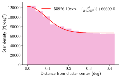
Figure 1: Stellar density in pragmatic units in annuli proceeding from the center of the sky position of NGC 7789. A Gaussian model is shown (red). Field star density is taken as the constant-density asymptote.

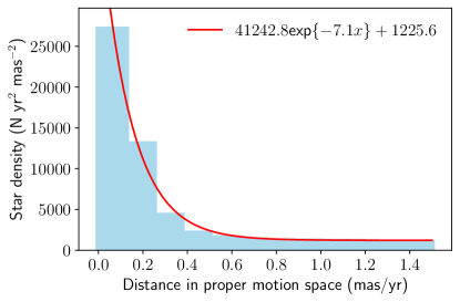
Figure 2: Stellar density in pragmatic units in annuli proceeding from the center of the proper motion location of NGC 7789 amongst the field stars. An exponential model is shown (red). Field star density is taken as the constant-density asymptote.

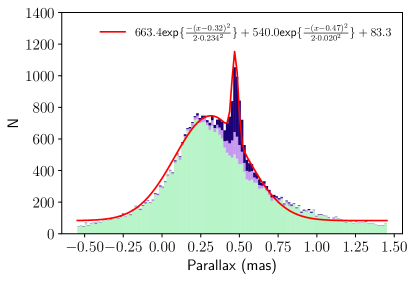
Figure 3: Distribution of stars in parallax in the NGC 7789 field. Stars nearest the proper motion locus (navy) and additional stars in a wider annulus (purple) form an obvious overdensity amongst the field stars (green). A two-Gaussian model is shown (red), with the broader component representing field stars.

Given three separate probability estimates, the combined probability from separate $P_{(\alpha,\delta)}$, $P_{\mu}$, and $P_{\pi}$ estimates is computed as in Balaguer-Núnez et al. (1998), updated to include increased dimensionality as in Griggio & Bedin (2022). The resultant probability distribution for NGC 7789 is shown in Fig. 4.

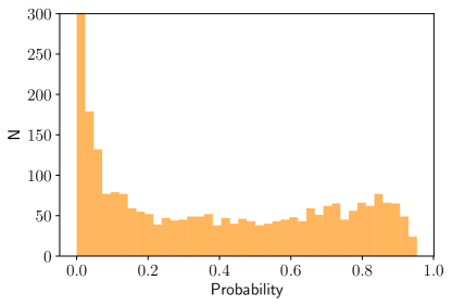
Figure 4: The resultant probability distribution after separate probabilities are combined for NGC 7789. The first bin contains about 20000 nonmember stars.

3 Results

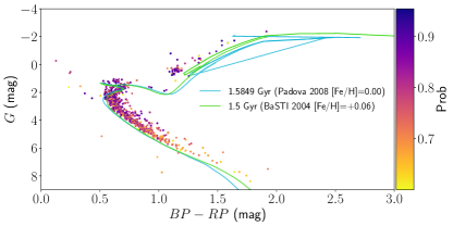
Figure 5: Color-absolute magnitude diagram in Gaia passbands for probable members ($P>0.7$) of NGC 7789 using the distance and reddening from Table 1. Symbols are color mapped by membership probability as indicated by the color bar. Example isochrones from Padova (blue, with carbon-rich stars excluded) and BaSTI (green) are shown.

From cleaned CMDs such as that of Fig. 5, we computed clump color-magnitude location using the Tukey biweight statistic (Beers et al., 1990) in both $BP-RP$ and $G$. The error in central location was estimated as $\sigma=\sqrt{v/N}$, where $v$ is the biweight midvariance and $N$ is the number of clump stars used for the calculation. Giant branch colors at the $G$ magnitude of the red clump were found by overlaying an isochrone’s RGB on the data. The synthetic RGB was then shifted left and right until 50% of stars were bluer and 50% of stars were redder. Once placed, the $BP-RP$ magnitude at the $G$ magnitude of the $RC$ was read from the shifted synthetic RGB. The clump stars outnumbered the RGB stars, so we expect counting statistics on the RGB to be the largest error source. We estimated RGB placement errors by shifting the theoretical RGB $\pm$ one star from the median position, and taking the average of the absolute value of those two shifts.

We adopted ages and rough age estimate errors from Cantat-Gaudin et al. (2020), namely $\pm$ 0.175 log years for clusters younger than 9.25 log years and $\pm$ 0.15 log years for older clusters. To plot H91’s data, we use the ages reported in the paper but scale them by 0.9 to approximately account for the drift in age scale from 1991 to now. We used the algebraic formulae in Riello et al. (2021) to transform from the Gaia photometric system to Johnson-Cousins $B-R$. Color excess from Kharchenko et al. (2013) was converted from E(B-V) to E($BP-RP$) using Casagrande & VandenBerg (2018).

Results are summarized in Table 1 and shown in Fig. 6 with the H91 fit, transformed to logarithmic age, overlaid.

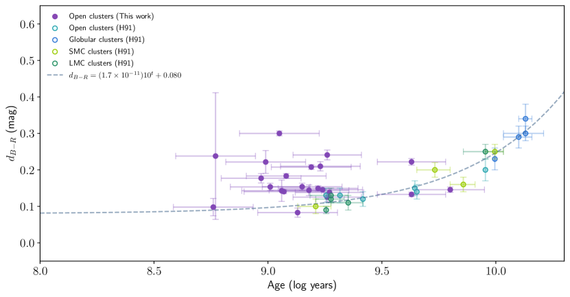
Figure 6: Color delta versus log age for open star clusters from this work (purple circles), along with open clusters (open blue-green circles), globular clusters (open blue circles), SMC clusters (open light green circles), and LMC clusters (open dark green circles) from H91. The H91 linear fit (dashed line) is also shown.

4 Discussion and Conclusion

From Fig. 6 we find that the H91 line extrapolates poorly at the young end, and that many clusters have a larger clump-RGB color separation than the relation would predict. At log(age) = 9.25, or age = 1.8 Gyr, the samples overlap in age, but every cluster in the new sample shows a wider $d_{B-R}$ color separation. The magnitude of the effect exceeds any possible random or systematic uncertainties.

Even restricted to the new measurements, and further restricted to log age $<9.5$, the scatter appears to be astrophysical. A Kolmogorov-Smirnov test on our $d_{BP-RP}$ values for clusters in our sample younger than 9.5 log years returned $p\approx 1.62\times 10^{-5}$, indicating that the scatter is not drawn from a normal distribution. The cause of the scatter cannot be age, or we would see a slope in Fig. 6. We sample metallicity span less well, but within that caveat, no metallicity dependence is evident. If neither age nor metallicity is the cause of the modulation in $d_{B-R}$, we are driven to consider more subtle causes such as variation in helium abundance, variation in the [$\alpha$/Fe] ratio, or variation in binary separation distributions. The investigation into the cause of the scatter must await future work.

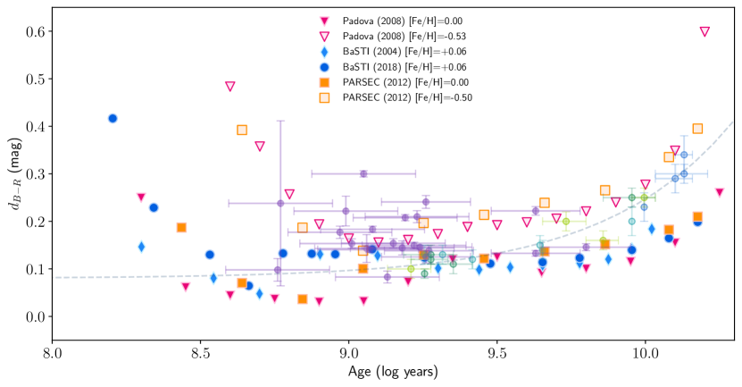
Figure 7: Color delta versus log age. Symbols are the same as Fig. 6 with the addition of predictions from various isochrone sets: We show (Marigo et al., 2008) at two abundance values (red triangles, unfilled for the metal poor sequence), BaSTI 5.0.1 (Pietrinferni et al., 2004) (blue diamonds), BaSTI (Hidalgo et al., 2018) (blue circles), and PARSEC+COLIBRI (Bressan et al., 2012) at two abundance values (orange squares, unfilled for the metal poor sequence).

We examine some predictions from stellar evolution theory in Fig. 7. All isochrones were translated from $T_{\rm eff}$ and log $L$ to $B-R$ using the empirical transformations of Worthey & Lee (2011). We show BaSTI 5.0.1 (Pietrinferni et al., 2004), BaSTI updated (Hidalgo et al., 2018), Padova, retrieved 2011 (Marigo et al., 2008), at two abundance values, and PARSEC+COLIBRI (Bressan et al., 2012) with Riemers (Reimers, 1977) $\eta=0.2$, retrieved 2023, also at two abundance values. On the positive side, all evolutionary sets are within $\sim$0.1 mag (about 150 K) of the observed color delta, and all sets show a growth in $d_{B-R}$ for ancient stellar populations that qualitatively mimics the observations.

If precision better than 150 K are desired, theory does not match observation. In particular, reading from Fig. 7, theory predicts a metallicity dependence of roughly $\frac{d(B-R)}{d{\rm[Fe/H]}}\geq-0.2$ mag per decade in heavy element abundance. A metallicity dependence this large is strictly ruled out by the data, which includes clusters from the large and small Magellanic Clouds. For example, super-metal-rich cluster NGC 6791 lies right among SMC clusters. The presence of this systematic among current isochrone sets affects CMD decompositions (Harris & Zaritsky, 2001; Dolphin, 2002). It also impacts integrated light models by introducing a fictitious color drift in the sense to make metal rich populations redder.

To estimate the size of the induced integrated light color change, we employ evolutionary population synthesis models (Worthey et al., 2022). As of this writing, these models have eight options for stellar evolution, but the earliest one (Worthey, 1994) uses the H91 scheme to place the red clump. We added an extra line of code to add a temperature shift, and translated the models that span metallicity in Fig. 7 from $\Delta$ color to $\Delta$ temperature via Worthey & Lee (2011). The results are summarized in Table 2. Because the main sequence dominates in the blue, $U-V$ is affected very little, but there is about a 4% effect in $V-K$.

Modelers should be aware of this discrepancy between current stellar evolution theory and observation because it adds to a list of ill-modeled or un-modeled effects that are far larger than the RMS fit between galaxy spectra and model integrated light spectra. Conroy et al. (2014), for example, find fits as good as 0.2% RMS, but their red clump temperatures do not adhere to H91 and so could be off by several percent. Blue stragglers are not included, which can lead to errors of over a magnitude in the terrestrial UV (Deng et al., 1999). Chemically peculiar stars, not included, alter the blue spectrum by $\sim$2% in the blue (Worthey & Shi, 2023). Binary evolution products, carbon stars, and metallicity-composite populations are likewise not modeled, and yet the optical spectrum matches to 0.2%. The reason the fit is excellent is a generalization the age-metallicity degeneracy (Worthey, 1994), where instead of age or metallicity, one inserts the concept of stellar temperatures in general. While some astrophysical inferences, such as abundance ratios, are somewhat isolated from this degeneracy, others, such as age, metallicity, age spread, or metallicity spread are not.

Table 2: Integrated light systematic color error if theoretical $Z$ dependence is allowed to flourish.

Quantity	log age	log age	log age
	= 9	= 9.5	= 10
$\Delta T_{\rm eff}$	172 K	93 K	212 K
$U-V$, MP, H91	0.75	1.11	1.43
$U-V$, MR, H91	1.04	1.58	1.99
$U-V$, MR, $+\Delta$theory	1.04	1.58	1.99
Excess $U-V$	0.004	0.002	0.003
$V-K$, MP, H91	2.39	2.73	3.04
$V-K$, MR, H91	2.70	3.33	3.81
$V-K$, MR, $+\Delta$theory	2.74	3.35	3.85
Excess $V-K$	0.038	0.021	0.037

Future work on red clump systematics might include cross matching Gaia’s star list with photometric catalogs with accuracies better than Gaia’s $BP-RP$. The costs might include possible loss of stars from the sample and also possible exposure to systematic error caused by transforming from heterogeneous photometric systems to a common one. To target more clusters might also be contemplated, but the key is to cover parameter space, and the present combined data of H91 and ourselves covers well what the Milky Way provides. The sample would benefit from the inclusion of SMC clusters younger than 1 Gyr. The SMC happens to have clusters aplenty at $\sim$650 Myr (Glatt et al., 2010). To explore to ages much younger than that is not appropriate, and there is a hard limit at $\sim$200 Myr. For ages less than $\sim$200 Myr, or, equivalently, MSTO masses greater than $\sim$5 M_⊙, stellar evolution through the RGB tip sparks no helium flash. The helium-burning “blue plumes” no longer resemble red clumps.

References

- Astropy Collaboration et al. (2013) Astropy Collaboration, Robitaille, T. P., Tollerud, E. J., et al. 2013, A&A, 558, A33, doi: 10.1051/0004-6361/201322068
- Astropy Collaboration et al. (2018) Astropy Collaboration, Price-Whelan, A. M., Sipőcz, B. M., et al. 2018, AJ, 156, 123, doi: 10.3847/1538-3881/aabc4f
- Astropy Collaboration et al. (2022) Astropy Collaboration, Price-Whelan, A. M., Lim, P. L., et al. 2022, ApJ, 935, 167, doi: 10.3847/1538-4357/ac7c74
- Balaguer-Núnez et al. (1998) Balaguer-Núnez, L., Tian, K. P., & Zhao, J. L. 1998, A&AS, 133, 387, doi: 10.1051/aas:1998324
- Beers et al. (1990) Beers, T. C., Flynn, K., & Gebhardt, K. 1990, AJ, 100, 32, doi: 10.1086/115487
- Bressan et al. (2012) Bressan, A., Marigo, P., Girardi, L., et al. 2012, MNRAS, 427, 127, doi: 10.1111/j.1365-2966.2012.21948.x
- Cantat-Gaudin et al. (2020) Cantat-Gaudin, T., Anders, F., Castro-Ginard, A., et al. 2020, A&A, 640, A1, doi: 10.1051/0004-6361/202038192
- Casagrande & VandenBerg (2018) Casagrande, L., & VandenBerg, D. A. 2018, MNRAS, 479, L102, doi: 10.1093/mnrasl/sly104
- Chaboyer (1995) Chaboyer, B. 1995, ApJ, 444, L9, doi: 10.1086/187847
- Conroy et al. (2014) Conroy, C., Graves, G. J., & van Dokkum, P. G. 2014, ApJ, 780, 33, doi: 10.1088/0004-637X/780/1/33
- Deng et al. (1999) Deng, L., Chen, R., Liu, X. S., & Chen, J. S. 1999, ApJ, 524, 824, doi: 10.1086/307832
- Dolphin (2002) Dolphin, A. E. 2002, MNRAS, 332, 91, doi: 10.1046/j.1365-8711.2002.05271.x
- Girardi (2016) Girardi, L. 2016, ARA&A, 54, 95, doi: 10.1146/annurev-astro-081915-023354
- Glatt et al. (2010) Glatt, K., Grebel, E. K., & Koch, A. 2010, A&A, 517, A50, doi: 10.1051/0004-6361/201014187
- Gratton et al. (2012) Gratton, R. G., Carretta, E., & Bragaglia, A. 2012, A&A Rev., 20, 50, doi: 10.1007/s00159-012-0050-3
- Griggio & Bedin (2022) Griggio, M., & Bedin, L. R. 2022, MNRAS, 511, 4702, doi: 10.1093/mnras/stac391
- Harris & Zaritsky (2001) Harris, J., & Zaritsky, D. 2001, ApJS, 136, 25, doi: 10.1086/321792
- Hatzidimitriou (1991) Hatzidimitriou, D. 1991, MNRAS, 251, 545, doi: 10.1093/mnras/251.4.545
- Hidalgo et al. (2018) Hidalgo, S. L., Pietrinferni, A., Cassisi, S., et al. 2018, ApJ, 856, 125, doi: 10.3847/1538-4357/aab158
- Kharchenko et al. (2013) Kharchenko, N. V., Piskunov, A. E., Schilbach, E., Röser, S., & Scholz, R. D. 2013, A&A, 558, A53, doi: 10.1051/0004-6361/201322302
- Marigo et al. (2008) Marigo, P., Girardi, L., Bressan, A., et al. 2008, A&A, 482, 883, doi: 10.1051/0004-6361:20078467
- Pietrinferni et al. (2004) Pietrinferni, A., Cassisi, S., Salaris, M., & Castelli, F. 2004, ApJ, 612, 168, doi: 10.1086/422498
- Reimers (1977) Reimers, D. 1977, A&A, 61, 217
- Riello et al. (2021) Riello, M., De Angeli, F., Evans, D. W., et al. 2021, A&A, 649, A3, doi: 10.1051/0004-6361/202039587
- Virtanen et al. (2020) Virtanen, P., Gommers, R., Oliphant, T. E., et al. 2020, Nature Methods, 17, 261, doi: 10.1038/s41592-019-0686-2
- Worthey (1994) Worthey, G. 1994, ApJS, 95, 107, doi: 10.1086/192096
- Worthey & Lee (2011) Worthey, G., & Lee, H.-c. 2011, ApJS, 193, 1, doi: 10.1088/0067-0049/193/1/1
- Worthey & Shi (2023) Worthey, G., & Shi, X. 2023, MNRAS, 518, 4106, doi: 10.1093/mnras/stac3297
- Worthey et al. (2022) Worthey, G., Shi, X., Pal, T., Lee, H.-c., & Tang, B. 2022, MNRAS, 511, 3198, doi: 10.1093/mnras/stac267