Brick Wall Quantum Circuits
with Global Fermionic Symmetry

Pietro Richelli^1,2,3, Kareljan Schoutens^1,2, Alberto Zorzato^1,2*

February 28, 2024

Abstract

We study brick wall quantum circuits enjoying a global fermionic symmetry. The constituent 2-qubit gate, and its fermionic symmetry, derive from a 2-particle scattering matrix in integrable, supersymmetric quantum field theory in 1+1 dimensions. Our 2-qubit gate, as a function of three free parameters, is of so-called free fermionic or matchgate form, allowing us to derive the spectral structure of both the brick wall unitary $\mathbf{U_{F}}$ and its, non-trivial, hamiltonian limit $\mathbf{H_{\gamma}}$ in closed form. We find that the fermionic symmetry pins $\mathbf{H_{\gamma}}$ to a surface of critical points, whereas breaking that symmetry leads to non-trivial topological phases. We briefly explore quench dynamics and entanglement build up for this class of circuits.

1 Introduction

1.1 Brick wall circuits and the choice of 2-qubit gate

A particularly fascinating interface of quantum information and quantum many-body physics is the study of quantum circuits that represent the (unitary) time evolution of systems in quantum particle or material physics. In their most basic form these circuits take the form of a ‘brick wall’ circuit whose properties are set by the choice of 2-qubit gate that represents a single brick in the wall. Studies of this type have typically opted for one of two extreme choices: either one assumes randomly chosen 2-qubit unitaries, or, on the opposite, one picks a structured 2-qubit gate that leads to a degree of analytical control of the unitary brick wall (UBW) circuit.

Indeed, if the 2-qubit gate is chosen to be a so-called $R$-matrix satisfying a Yang-Baxter identity, one can arrange a corresponding UBW circuit such that, as an operator, it commutes with a large number of conserved charges. See [9, 25] where this procedure was proposed and analyzed and [26] where such circuits, and the corresponding idea of ‘integrable trotterization’ was studied. Ref [14] in particular has implemented these ideas for the $R$-matrix of the XXX integrable spin-$1/2$ Heisenberg magnet and analyzed its conserved charges, both analytically and in realizations on quantum computing hardware.

Most studies of this type feature an $R$-matrix characterized by a $U(1)$ symmetry (as in the XXZ models) or an $SU(2)$ symmetry (as in the XXX magnet), exploiting the fact that these symmetries are natural (or even native) to qubit based quantum processors. The starting point for our investigations in this paper is another notion of symmetry that is natural for 2-state systems, namely a fermionic symmetry that rotates $\ket{0}$ to $\ket{1}$. This interpretation assumes that we can treat a multi-qubit register as a graded tensor product of 1-qubit states, which means that certain minus signs have to be in place.

1.2 2-Qubit gates from supersymmetric particle scattering

A context where solutions to a Yang-Baxter equation arise in a natural way is that of factorizable particle scattering in massive integrable quantum field theories (QFT) in 1+1 dimensions. These theories describe (massive) particles in 1+1D, whose many-body scattering processes factor into 2-body processes as a consequence of integrability. In the early 1990’s a great number of non-trivial such $S$-matrices were identified through the study of QFT’s arising from relevant, integrable perturbations of conformal field theories (CFT), or from direct analysis of integrable QFT’s such as the sine-Gordon model. A highlight of the former approach has been the identification of the $S$-matrices for massive particles arising from the magnetic perturbation of the Ising CFT, with the masses and the scattering matrices all organized by an underlying $E_{8}$ symmetry [30].

In 1+1D QFT context the notion of a fermionic symmetry of a 2-body scattering matrix takes the form of space-time supersymmetry [19]. It expresses the 1+1D super Poincaré algebra, in the form

$$\mathcal{Q}^{2}=\mathcal{P},\quad\mathcal{\overline{Q}}^{2}=\mathcal{\overline{P}},\quad\mathcal{P}^{0}=\mathcal{P}+\mathcal{\overline{P}},\quad\mathcal{P}^{1}=\mathcal{P}-\mathcal{\bar{P}}$$ (1.1)

with the energy $\mathcal{P}^{0}$ and momentum $\mathcal{P}^{1}$ operators taking values

$$p^{0}=m\cosh(\theta),\quad p^{1}=m\sinh(\theta)$$ (1.2)

for on-shell particles with mass $m$ and rapidity $\theta$. In such supersymmetric QFT’s, particles come in doublets $(b_{i},f_{i})$ of mass $m_{i}$, giving rise to (asymptotic) particle states

$$\ket{A_{i_{1}}(\theta_{1})\ldots A_{i_{n}}(\theta_{n})}$$ (1.3)

with $A_{i}=b_{i},\,f_{i}$. A particularly natural choice for the action of the supercharges is, in matrix form,

$$Q=\sigma_{x},\quad\overline{Q}=\sigma_{y},\quad Q_{L}=\sigma_{z},$$ (1.4)

with $Q_{L}$ representing the parity operator. On a 2-particle state the supercharges then act as

$$\mathbf{Q^{l}}=\sqrt{m_{1}}\,e^{\theta_{1}/2}Q\otimes{\rm I}+\sqrt{m_{2}}\,e^{\theta_{2}/2}Q_{L}\otimes Q$$ (1.5)

and similar for $\mathbf{Q^{r}}$ (in terms of $\overline{Q}$). Note that the operator $Q_{L}$ in the second term expresses the fermionic nature of the supercharges.

The paper [19] identified the most general 2-body $S$-matrix commuting with this particular representation of space-time supersymmetry. Written on the basis $\ket{b_{i}(\theta_{1})b_{j}(\theta_{2})}$, $\ket{b_{i}(\theta_{1})f_{j}(\theta_{2})}$, $\ket{f_{i}(\theta_{1})b_{j}(\theta_{2})}$, $\ket{f_{i}(\theta_{1})f_{j}(\theta_{2})}$, it takes the form

$$\mathbf{\check{S}}(\theta)=f(\theta)\left(\begin{matrix}1-t\,\tilde{t}&0&0&t+\tilde{t}\\ 0&1+t\,\tilde{t}&t-\tilde{t}&0\\ 0&-t+\tilde{t}&1+t\,\tilde{t}&0\\ -t-\tilde{t}&0&0&1-t\,\tilde{t}\end{matrix}\right)+g(\theta)\left(\begin{matrix}1&0&0&0\\ 0&0&1&0\\ 0&1&0&0\\ 0&0&0&-1\end{matrix}\right).$$ (1.6)

The dependence on $\theta=\theta_{1}-\theta_{2}$ and the different masses is through the parameters

$$t=\tanh\left[\frac{\theta+\gamma}{4}\right],\quad\tilde{t}=\tanh\left[\frac{\theta-\gamma}{4}\right],\qquad{\rm with}\ \gamma=\log\left(\frac{m_{i}}{m_{j}}\right).$$ (1.7)

The functions $f(\theta)$ and $g(\theta)$ are related as

$$f(\theta)=\frac{\alpha}{2i}\sqrt{m_{i}m_{j}}\frac{\cosh(\theta/2)+\cosh(\gamma/2)}{\cosh(\theta/2)\sinh(\theta/2)}g(\theta).$$ (1.8)

The parameter $\alpha>0$ sets the strength of the Bose-Fermi mixing interactions: for $\alpha=0$ the transformations $\ket{b}\to\ket{f}$ and $\ket{f}\to\ket{b}$ are not allowed, and the scattering matrix reduces to a graded permutation, $\mathbf{\check{S}}=\mathbf{\Pi}$. The overall normalization $g(\theta)$ provided in [19] is particular to the 1+1D scattering context and not important here. For $\mathbf{\check{S}}(\theta)$ to be unitary we choose $g(\theta)$ as

$$g(\theta)=i\left(1+2\alpha^{2}\frac{\cosh(\theta)+\cosh(\gamma)}{\sinh^{2}(\theta)}\right)^{-1/2}.$$ (1.9)

The paper [19] showed that, without any further restrictions, these scattering matrices satisfy the Yang-Baxter relation. The same paper identified concrete examples of integrable supersymmetric perturbations of supersymmetric CFT, with $S$-matrices given by eq. 1.6. The simplest, featuring a single doublet $(b,f)$, starts from a CFT with central charge $c=-21/4$, and provides a supersymmetric analogue of the scattering theory arising from a perturbation of the CFT going with the Yang-Lee edge singularity at $c=-22/5$ [3]. A later paper [17] confirmed this identification with the help of a Thermodynamic Bethe Ansatz (TBA) procedure.

Back to the subject of the current paper: taking $\mathbf{\check{S}}(\theta)$ (properly normalized) as our fundamental 2-qubit gate, we build and analyze a class of UBW circuits that are naturally endowed with a graded tensor product structure, integrability and a global fermionic symmetry having its origin in space-time supersymmetry in 1+1D.

Before delving into this, we remark that, if we wish to study UBW circuits with open boundary conditions (OBC), we will need boundary operators that respect the fermionic symmetry. Such boundary reflection operators were found and studied in [16]. On the 1-particle states $\ket{b(\theta)}$, $\ket{f(\theta)}$ they take the concrete form

$$\mathbf{K}(\theta)=\sqrt{\frac{2}{\cosh(\theta)}}\left(\begin{matrix}\cosh(\theta/2-i\pi/4)&0\\ 0&\cosh(\theta/2+i\pi/4)\end{matrix}\right)$$ (1.10)

and satisfy

$$\mathbf{Q}(-\theta)\mathbf{K}(\theta)=\mathbf{K}(\theta)\mathbf{Q}(\theta),$$ (1.11)

with $\mathbf{Q}=\mathbf{Q^{l}}+\mathbf{Q^{r}}$. Thus, the boundary reflection operators commute with the sum of the left and right supercharges.

1.3 Free fermion structure and matchgate condition

It has been observed and employed early on [7, 5, 6, 17] that the matrix $\mathbf{\check{S}}(\theta)$ in eq. 1.6, parameterized by $\alpha$ and $\gamma$ and viewed in the context of a statistical mechanics model, satisfies a ‘free fermion condition’. In the language of quantum information, it is said that the corresponding 2-qubit gate is a so-called matchgate. Following the definition in [21], a matchgate is a 2-qubit gate which in the computational basis takes the form

$$G(A,B) =\left(\begin{matrix}p&0&0&q\\ 0&w&x&0\\ 0&y&z&0\\ r&0&0&s\end{matrix}\right) A =\left(\begin{matrix}p&q\\ r&s\end{matrix}\right) B =\left(\begin{matrix}w&x\\ y&z\end{matrix}\right),$$ (1.12)

where $A$ and $B$ are both elements of $SU(2)$ or $U(2)$ and they have the same determinant. Our matrix $\mathbf{\check{S}}(\theta)$ is precisely of this form.

The free fermion or matchgate condition guarantees that the matrix $\mathbf{\check{S}}(\theta)$ can be written as the exponent of a bilinear in free fermion creation and annihilation operators, see eq. 2.18 below.

This observation explains the fact that $\mathbf{\check{S}}(\theta)$ satisfies the Yang-Baxter relations. It also confirms the original observation that the scattering matrix $\mathbf{\check{S}}(\theta)$ is best understood in fermionic language. This however presupposes that a Jordan-Wigner transformation connecting back to bosonic qubits is in place. This is a concern in particular in the case where periodic boundary condition (PBC) are imposed, as the matrix $\mathbf{\check{S}}(\theta)_{L1}$ (see figure 1(a)) connecting the outer qubits numbered as $L$ and $1$ depends on the total parity of the state carried by qubits $2,\ldots,L-1$. See section 2.2 for a discussion of this point.

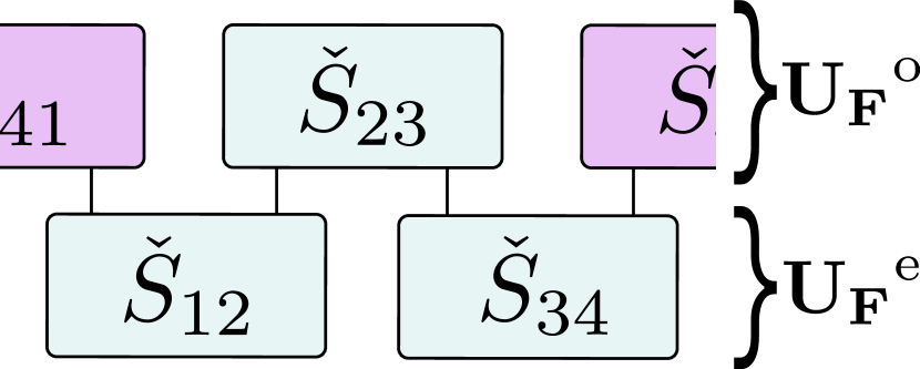
(a) PBC circuit

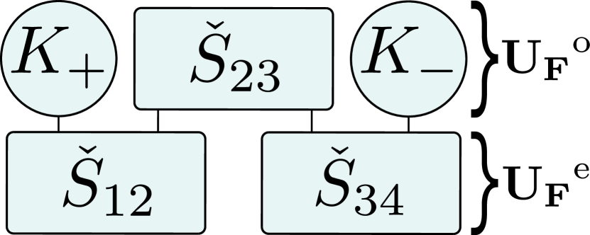
(b) OBC circuit

Figure 1: PBC/OBC single-layer circuits for a 4-site system

The free fermion or matchgate condition also implies that (under mild conditions, see [21]) UBW circuits based on $\mathbf{\check{S}}(\theta)$ can be simulated efficiently in polynomial time on a classical computer [10, 21, 23]. In addition, the unitary operator represented by a UBW can be represented as

$$\mathbf{U_{F}}(\theta)=\exp[i\mathbf{E}(\theta)]=\exp\left[i\sum_{j}\epsilon_{j}(\eta_{j}^{\dagger}\eta_{j}-\frac{1}{2})\right],$$ (1.13)

where $\eta^{\dagger}_{j}$ and $\eta_{j}$ are linear combinations of the 1-qubit creation and annihilation operators $c^{\dagger}_{j}$ and $c_{j}$, and the $\epsilon_{j}$ are 1-particle energies. Explicitly analyzing this expression in a momentum basis, and computing the dispersion relations $\epsilon_{j}^{k}$, is among the most important goals of this paper.

We remark that the matrices $\mathbf{\check{S}}(\theta)$ , which we identified by imposing a global fermionic symmetry, are not the most general matrices satisfying a free fermion or matchgate condition. We point out [18] for a recent analysis of quantum circuits with underlying free fermionic structure. We can thus study the breaking of the fermionic symmetry without leaving the space of free fermion (matchgate) gates. As explained below, we will find that, typically, imposing the global fermionic symmetry will force a gapless dispersion and hence critical behaviour in the corresponding quantum dynamics. Breaking that symmetry typically leads to topologically non-trivial phases protected by a gap.

UBW circuits based on an $R$-matrix of XXZ type similarly have a free fermion point. That point enjoys a $U(1)$ symmetry, allowing to solve for the dispersions $\epsilon_{i}^{k}$ by solving a quadratic equation [26]. In our situation only a $\mathbf{Z}_{2}$ symmetry (the fermion parity) survives, implying that our dispersions obey quartic equations at best. This then translates into a richer dependence of the $\epsilon_{i}^{k}$ on the momentum $k$. As an example, we identify situations with two critical modes, one with dispersion linear in $k$ and the other with cubic $(\propto k^{3})$ dispersion.

2 Brick wall circuits: preliminaries

Quantum brick wall circuits have been studied in depth in recent years. Here we propose their fermionic extension, meaning that we treat our multi-qubit register as a graded Hilbert space and trade the Pauli spin operators for their fermionic counterparts.

2.1 Graded tensor product

In order to properly introduce what we will call a graded brick wall we first need to outline the main properties of graded vector spaces, the content of this subsection is mainly taken from [4]. We will focus on 2 dimensional graded vector spaces $V^{g}\cong\mathbb{C}^{(1|1)}\cong\mathbb{C}\oplus\mathbb{C}$ with basis $\{e_{0},\,e_{1}\}$. A graded space is characterized by a parity function $p:V^{g}\to\mathbb{Z}_{2}$ that acts on the basis space as:

$$p(e_{0})=0 p(e_{1})=1$$ (2.1)

Naturally the permutation operator defined on graded spaces is different than the usual, thus we will denote it with $\mathbf{\Pi}$. On two vectors $v,\,w\in\mathbb{C}^{(1|1)}$ acts in the following way:

$$\mathbf{\Pi}(e_{i}\otimes e_{j})=(-1)^{p(e_{i})p(e_{j})}e_{j}\otimes e_{i} \forall i,\,j\in\mathbb{Z}_{2}$$ (2.2)

The last necessary notion about graded vector spaces is the graded tensor product. The parity operator is essential to define the tensor product in graded spaces, in fact taken two vectors $v,\,w\in\mathbb{C}^{(1|1)}$ then their tensor product will live in the space $\mathbb{C}^{(1|1)}\otimes\mathbb{C}^{(1|1)}$ and it will be:

$$v\otimes w=v_{i}e_{i}\otimes w_{j}e_{j}=(e_{i}\otimes e_{j})\,v_{i}w_{j}{(-1)}^{p(v_{i})p(e_{j})}\,.$$ (2.3)

The graded tensor product can be extended on the space of endomorphisms $\mathrm{End}(\mathcal{H})$, with $\mathcal{H}\cong\bigotimes_{i}V^{g}_{i}$. Given $\mathcal{H}\cong V^{g}_{1}\otimes\dots\otimes V^{g}_{N}$, a local operator on the subspace $V^{g}_{i}$ is defined as:

$$\left(\hat{O}_{i}\right)_{\mathbf{b}}^{\mathbf{a}}=(-1)^{\sum_{j<i}p(a_{j})(a_{i}+b_{i})}\mathbb{1}\otimes\dots\otimes\mathbb{1}\otimes\hat{O}_{i}\otimes\mathbb{1}\otimes\dots\otimes\mathbb{1}\,,$$ (2.4)

where $\mathbf{a}=(a_{1},\dots,a_{n})$ and $\mathbf{b}=(b_{1},\dots,b_{n})$ are, respectively, two vectors that denote the rows and columns of the subspace $V^{g}_{i}$. With this notation we can extend the parity operator to $\mathrm{End}(\mathcal{H})$ with $\mathcal{H}\cong\bigotimes_{i}V^{g}_{i}$ as:

Definition 2.1 (Operator parity).

Given an operator $S\in\mathrm{End}\left(V_{1}\otimes\dots\otimes V_{n}\right)$ its parity is defined as:

$$p\left(S_{\mathbf{b}}^{\mathbf{a}}\right)=\sum_{i=1}^{n}a_{i}+b_{i}\mod 2\,.$$ (2.5)

For 2 dimensional graded vector spaces the graded tensor product gives an immediate representation into the non graded vector space. Considering a local operator as in equation 2.4, the operator parity in 2.5 and that any operator can be written as a linear combination of an even an an odd part $\hat{O}=\alpha\hat{O}^{e}+\beta\hat{O}^{o}$, for the even part $p(\hat{O})=0$ we can write

$$\hat{O}^{e}_{i}=\mathbb{1}\otimes\dots\otimes\mathbb{1}\otimes\hat{O}^{e}_{i}\otimes\mathbb{1}\otimes\dots\otimes\mathbb{1}\,,$$ (2.6)

and for the odd part $p(\hat{O})=1$,

$$\hat{O}^{o}_{i}=\sigma^{z}\otimes\dots\otimes\sigma^{z}\otimes\hat{O}^{o}_{i}\otimes\mathbb{1}\otimes\dots\otimes\mathbb{1}\,.$$ (2.7)

Therefore in our brick wall there will be strings of $\sigma^{z}$ operator that appear in the ungraded representation of the graded operators. Although seemingly a complication, the non locality that will characterize our circuit is the same we have to deal with once we take a Jordan-Wigner transformation. The boundary term $(-1)^{\hat{N}}$ that naturally appears in the Jordan-Wigner transformation will be cancelled by the string of $\sigma^{z}$ given by the graded tensor product. This peculiar feature makes our system fermionic and it shows how the supersymmetry present in the field theory translates into what we call global fermionic symmetry.

2.2 PBC: UBW and graded Floquet Baxterization

To set up our brick wall circuits, we assume particles of mass $m_{1}$ and rapidity $\theta_{1}=\theta/2$ on the odd qubit lines, and particles of mass $m_{2}$ and rapidity $\theta_{2}=-\theta/2$ on the even lines, in agreement with [15]. This leads to the following unitary operator, which we will loosely refer to as a time evolution operator,

$$\mathbf{U_{F}}(\alpha,\gamma,\theta)=\mathbf{U_{F}}^{\mathrm{o}}(\alpha,\gamma,\theta)\mathbf{U_{F}}^{\mathrm{e}}(\alpha,\gamma,\theta)=\left(\prod_{i=1}^{L/2}\mathbf{\check{S}}_{2i,2i+1}(\theta)\right)\left(\prod_{i=1}^{L/2}\mathbf{\check{S}}_{2i-1,2i}(\theta)\right)\,,$$ (2.8)

where $\mathbf{\check{S}}(\theta)$ is the unitary gate defined by equation 1.6, with $\theta=\theta_{1}-\theta_{2}$. We put $m_{1}m_{2}=1$, absorbing the overall mass scale in $\alpha$. We will refer to a single application of $\mathbf{U_{F}}(\alpha,\gamma,\theta)$ as one single layer, comprised of two sublayers (even $\mathbf{U_{F}}^{\mathrm{e}}(\alpha,\gamma,\theta)$ and odd $\mathbf{U_{F}}^{\mathrm{o}}(\alpha,\gamma,\theta)$).

In [15] it was shown that a brick wall circuit of this type is integrable if $\mathbf{S}=\mathbf{P}\,\mathbf{\check{S}}$ satisfies the Yang-Baxter equations. Thus a transfer matrix can be constructed as

$$\mathbf{t}(u,\theta_{1},\theta_{2})=\mathrm{Tr}_{a}\left[\prod_{i}^{L}\mathbf{S}_{a,i}(u-\theta_{j})\right]\,, j=i\mod 2+1\,,$$ (2.9)

such that is satisfies the following commutation relations

$$\left[\mathbf{t}(u,\theta_{1},\theta_{2}),\mathbf{t}(v,\theta_{1},\theta_{2})\right]\,, \left[\mathbf{U_{F}}(\theta),\mathbf{t}(u,\theta_{1},\theta_{2})\right]\,, \forall u,\,v\in\mathbb{C}\,,$$ (2.10)

The integrability of the brick wall circuit was proved only for standard Hilbert spaces without grading, therefore we need to extend this result to graded Hilbert spaces. The statement and proof of a graded Floquet Baxterization theorem can be found in Appendix A. Since the scattering matrix 1.6 is free fermionic we will not need the theorem in the current analysis, but it will be useful for future works on non free-fermionic models.

The scattering matrix is defined on the tensor product of graded Hilbert spaces, thus in equation 2.8 there is an implicit graded tensor product. Since $p(\mathbf{\check{S}})=0$ there will be no sign correction for all operators but $\mathbf{\check{S}}_{L,1}(\theta)$. In fact the off-diagonal elements, which can be written as linear combinations of $\sigma^{x}$ and $\sigma^{y}$, will be of the form:

$$\sigma^{\alpha}_{1}\left(\prod_{i=2}^{L-1}\sigma^{z}_{i}\right)\sigma^{\beta}_{L}\,, \alpha\,,\beta=x,y$$ (2.11)

These terms under a Jordan-Wigner transformation become nearest neighbour interactions without any sign correction of the form $(-1)^{\hat{N}}$, as discussed previously.
The global fermionic symmetry of the brick wall circuit is inherited from the supersymmetry of the scattering matrix in equation 1.6. Generalising the supercharges to a $L$ particle space in the following way

$$\mathbf{Q^{L}}(\gamma,\theta)=\sum_{i=1}^{L/2}\mathbf{Q^{l}}_{2i-1,2i}(\gamma,\theta)\,, \mathbf{Q^{R}}(\gamma,\theta)=\sum_{i=1}^{L/2}\mathbf{Q^{r}}_{2i-1,2i}(\gamma,\theta)\,,$$ (2.12)

where

$$\mathbf{Q^{l}}_{2i-1,2i}(\gamma,\theta) =e^{\frac{\gamma+\theta}{4}}\left(\prod_{j<2i-1}\sigma_{j}^{z}\right)\sigma_{2i-1}^{x}+e^{-\frac{\gamma+\theta}{4}}\left(\prod_{j<2i}\sigma_{j}^{z}\right)\sigma_{2i}^{x}\,,$$ (2.13)

$$\mathbf{Q^{r}}_{2i-1,2i}(\gamma,\theta) =e^{\frac{\gamma-\theta}{4}}\left(\prod_{j<2i-1}\sigma_{j}^{z}\right)\sigma_{2i-1}^{y}+e^{-\frac{\gamma-\theta}{4}}\left(\prod_{j<2i}\sigma_{j}^{z}\right)\sigma_{2i}^{y}\,.$$ (2.14)

we find

$$\mathbf{Q^{L/R}}(\theta)\mathbf{U_{F}}(\theta) =\mathbf{Q^{L/R}}(\theta)\mathbf{U}^{\mathrm{o}}_{\mathbf{F}}(\theta)\mathbf{U}^{\mathrm{e}}_{\mathbf{F}}(\theta)\,,$$

$$=\mathbf{U}^{\mathrm{o}}_{\mathbf{F}}(\theta)\mathbf{Q^{L/R}}(-\theta)\mathbf{U}^{\mathrm{e}}_{\mathbf{F}}(\theta)\,,$$

$$=\mathbf{U}^{\mathrm{o}}_{\mathbf{F}}(\theta)\mathbf{U}^{\mathrm{e}}_{\mathbf{F}}(\theta)\mathbf{Q^{L/R}}(\theta)\,,$$

$$=\mathbf{U_{F}}(\theta)\mathbf{Q^{L/R}}(\theta)\,.$$ (2.15)

The strings of $\sigma^{z}$ in 2.14 show the fermionic nature of the operators, each single term in the two sums 2.12 becomes local after a Jordan-Wigner transformation. A single operator does not commute with the time evolution operator, therefore the support of the two operators $\mathbf{Q^{L/R}}(\gamma,\theta)$ is the whole chain.

2.3 OBC: UBW and fermionic symmetry

A unitary brick wall circuit with open boundary condition (OBC) and global fermionic symmetry can be realized by employing the boundary scattering operators $\mathbf{K(\theta)}$ displayed in eq. 1.10. However, for the general case with $m_{1}\neq m_{2}$ this will take a circuit with $L$ layers rather than 1 layer.

Let us illustrate this for the case $L=4$, see also fig. 1(b). The natural definition of a UBW circuit with OBC is

$$\mathbf{U_{F}^{\rm OBC}}(\alpha,\gamma,\theta)=\left[\mathbf{K_{1}(-\theta/2)}\mathbf{\check{S}}_{2,3}(\alpha,\gamma,\theta)\mathbf{K_{4}(\theta/2)}\right]\left[\mathbf{\check{S}}_{1,2}(\alpha,\gamma,\theta)\mathbf{\check{S}}_{3,4}(\alpha,\gamma,\theta)\right].$$ (2.16)

A layer is made of two sublayers (see figure 1(b)), where in the second sublayer the particles at sites 1 and 4 reflect off the open boundaries. For equal masses, $\gamma=0$, one quickly checks that $\mathbf{U_{F}^{\rm OBC}}(\alpha,\gamma,\theta)$ commutes with $\mathbf{Q^{L}}(\theta)+\mathbf{Q^{R}}(\theta)$.

However, for $m_{1}\neq m_{2}$ the operator $\mathbf{U_{F}^{\rm OBC}}(\alpha,\gamma,\theta)$ leaves the system in a configuration where sites 1 and 2 have a particle of mass $m_{2}$ while sites 3 and 4 have a particle of mass $m_{1}$. On such a state $\mathbf{Q^{L}}(\theta)+\mathbf{Q^{R}}(\theta)$ (which assumes that the particles alternate between $m_{1}$ and $m_{2}$ along the chain) is not an appropriate operator. To return to the original configuration of particle masses and rapidities, we need an extended UBW which comprises not 1 but $L=4$ layers,

$$\mathbf{U_{F}^{\rm OBC,extended}}(\alpha,\gamma,\theta)=$$ (2.17)

$$\left[\mathbf{K_{1}(-\theta/2)}\mathbf{\check{S}}_{2,3}(\alpha,\gamma,\theta)\mathbf{K_{4}(\theta/2)}\right]\left[\mathbf{\check{S}}_{1,2}(\alpha,0,\theta)\mathbf{\check{S}}_{3,4}(\alpha,0,\theta)\right]$$

$$\times\left[\mathbf{K_{1}(-\theta/2)}\mathbf{\check{S}}_{2,3}(\alpha,-\gamma,\theta)\mathbf{K_{4}(\theta/2)}\right]\left[\mathbf{\check{S}}_{1,2}(\alpha,-\gamma,\theta)\mathbf{\check{S}}_{3,4}(\alpha,-\gamma,\theta)\right]$$

$$\quad\times\left[\mathbf{K_{1}(-\theta/2)}\mathbf{\check{S}}_{2,3}(\alpha,-\gamma,\theta)\mathbf{K_{4}(\theta/2)}\right]\left[\mathbf{\check{S}}_{1,2}(\alpha,0,\theta)\mathbf{\check{S}}_{3,4}(\alpha,0,\theta)\right]$$

$$\quad\quad\times\left[\mathbf{K_{1}(-\theta/2)}\mathbf{\check{S}}_{2,3}(\alpha,\gamma,\theta)\mathbf{K_{4}(\theta/2)}\right]\left[\mathbf{\check{S}}_{1,2}(\alpha,\gamma,\theta)\mathbf{\check{S}}_{3,4}(\alpha,\gamma,\theta)\right].$$

This operator, by construction, commutes with $\mathbf{Q^{L}}(\gamma,\theta)+\mathbf{Q^{R}}(\gamma,\theta)$.

2.4 Free Fermi form of the scattering matrix

The hidden free fermionic (or matchgate) structure that we discussed in section 1.3 guarantees that the 2-body scattering operator, which furnishes our basic 2-qubit gate, can be written in free fermionic form. We display this form in this section and shall extend it to the many-body UBW in section 4 below. We start by expressing $\mathbf{\check{S}}(\alpha,\gamma,\theta)$ in exponential form

$$\mathbf{\check{S}}_{i,i+1}(\alpha,\gamma,\theta)=\exp[i\mathbf{E}_{i,i+1}].$$ (2.18)

The two-site exponent $\mathbf{E}_{i,i+1}$ can be written as a linear combination of tensor products of Pauli matrices, resulting in

$$\begin{split}\mathbf{E}_{i,i+1}&=\frac{a_{11}}{2}\left(\sigma_{i}^{z}+\sigma_{i+1}^{z}\right)+\frac{a_{12}}{2}\cos(\phi)\left(\sigma_{i}^{x}\sigma_{i+1}^{x}+\sigma_{i}^{y}\sigma_{i+1}^{y}\right)\\ &\qquad-\frac{a_{12}}{2}\sin(\phi)\left(\sigma_{i}^{x}\sigma_{i+1}^{y}-\sigma_{i}^{y}\sigma_{i+1}^{x}\right)+\frac{b_{12}}{2}\left(\sigma_{i}^{x}\sigma_{i+1}^{y}+\sigma_{i}^{y}\sigma_{i+1}^{x}\right)\end{split}$$ (2.19)

The coefficients are found to be the following

$$a_{11} =\frac{\sqrt{2}\cosh\left(\frac{\theta}{2}\right)}{\sqrt{2\alpha^{2}+\cosh(\theta)+1}}\arccos\left(\frac{2\alpha\cosh\left(\frac{\gamma}{2}\right)}{\sqrt{2\alpha^{2}(\cosh(\gamma)+\cosh(\theta))+\sinh^{2}(\theta)}}\right),$$

$$a_{12} =\arccos\left(\frac{2\alpha\cosh(\frac{\theta}{2})}{\sqrt{2\alpha^{2}(\cosh(\gamma)+\cosh(\theta))+\sinh^{2}(\theta)}}\right),$$

$$\phi =\frac{1}{2}\arccos\left(\frac{\sinh^{2}(\theta)-4\alpha^{2}\sinh^{2}(\frac{\gamma}{2})}{\sinh^{2}(\theta)+4\alpha^{2}\sinh^{2}(\frac{\gamma}{2})}\right),$$

$$b_{12} =\frac{\sqrt{2}\alpha}{\sqrt{2\alpha^{2}+\cosh(\theta)+1}}\arccos\left(\frac{2\alpha\cosh\left(\frac{\gamma}{2}\right)}{\sqrt{2\alpha^{2}(\cosh(\gamma)+\cosh(\theta))+\sinh^{2}(\theta)}}\right).$$ (2.20)

Now we can use the Jordan-Wigner transformation to express our exponent in terms of spinless fermionic operators,

$$c_{i}^{\dagger}=\prod_{j<i}\sigma_{j}^{z}\sigma_{i}^{-}\,, c_{i}=\prod_{j<i}\sigma_{j}^{z}\sigma_{i}^{+}\,, \sigma^{z}_{i}=\mathbb{1}-2c_{i}^{\dagger}c_{i}\,.$$ (2.21)

This leads to

$$\begin{split}\mathbf{E}_{i,i+1}&=-a_{11}\left(c_{i}^{\dagger}c_{i}+c_{i+1}^{\dagger}c_{i+1}-\mathbb{1}\right)+a_{12}\left(e^{i\phi}c_{i}^{\dagger}c_{i+1}+e^{-i\phi}c_{i+1}^{\dagger}c_{i}\right)\\ &\qquad+ib_{12}\left(c_{i}^{\dagger}c_{i+1}^{\dagger}-c_{i+1}c_{i}\right)\,.\end{split}$$ (2.22)

This form makes clear that we can consider free fermionic 2-qubit gates that venture outside the space parametrized by $\alpha$, $\gamma$, $\theta$, where a global fermionic symmetry is enforced. We will later see that these correspond to breaking criticality and give rise to topological phases in the hamiltonian limit of the UBW.

2.5 UBW and hamiltonian limit

While we loosely think of $\mathbf{U_{F}}(\alpha,\gamma,\theta)$ as a time evolution operator, with $\theta$ taking the role of time, we should realize that the eigenvalues of $\mathbf{E}_{i,i+1}$ depend on $\theta$ in a non-linear fashion. A standard picture of quantum mechanical time evolution arises in the limit of small $\theta$ and for $\gamma=0$. Since $\mathbf{U_{F}}(\alpha,\gamma=0,\theta=0)$ is the identity operator, the behaviour of $\mathbf{U_{F}}$ in this limit is fully captured by its logarithmic derivative, which we call $\mathbf{H_{0}}(\alpha)$ (section 3.1).

For $\gamma\neq 0$ the $\theta\to 0$ limit of $\mathbf{U_{F}}(\alpha,\gamma,\theta)$ is not the identity and we should prepend a circuit representing $\mathbf{U_{F}}(\alpha,\gamma,0)^{-1}$ before we can extract a logarithmic derivative, which we will call $\mathbf{H_{\gamma}}(\alpha,\gamma)$ (sections 3.2 and 3.3).

The global fermionic symmetry of $\mathbf{U_{F}}(\alpha,\gamma,\theta)$ carries over to both $\mathbf{H_{0}}(\alpha)$ and $\mathbf{H_{\gamma}}(\alpha,\gamma)$. We will find that this implies that these hamiltonians are critical for all $\alpha$, $\gamma$.

3 Brick wall circuit in the hamiltonian limit

For general $\alpha$, $\gamma$, we can write the following expansion of the Floquet time evolution operator for $\theta\to 0$,

$$\mathbf{U_{F}}(\theta)=\exp[i\mathbf{E}(\theta)]\overset{\theta\to 0}{=}\mathbf{U_{F}}(0)+i\mathbf{U_{F}}(0)\mathbf{H_{\gamma}}(\theta)+o(\theta^{2})\,,$$ (3.1)

defining $\mathbf{H_{\gamma}}$ as the logarithmic derivative of $\mathbf{U_{F}}(0)^{-1}\mathbf{U_{F}}(\theta)$. We first we look at the simpler case with $\gamma=0$.

3.1 $\gamma=0$

For $\gamma=0$ the scattering matrix (S-matrix) becomes the identity operator, $\mathbf{\check{S}}(\alpha,0,0)=\mathbb{1}$, thus the only relevant operator will be its first order derivative,

$$\mathbf{\check{S}}(\alpha,0,\theta)\overset{\theta\to 0}{=}\mathbb{1}+i\left(\begin{matrix}\frac{1}{2\alpha}&0&0&\frac{-i}{2}\\ 0&0&\frac{1}{2\alpha}&0\\ 0&\frac{1}{2\alpha}&0&0\\ \frac{i}{2}&0&0&-\frac{1}{2\alpha}\end{matrix}\right)\theta+o(\theta^{2})\,.$$ (3.2)

The logarithmic derivative in equation 3.1 can be analytically derived,

$$\mathbf{H_{0}}(\alpha)=\left.\frac{\partial}{\partial\theta}\mathbf{E}(\theta)\right|_{\theta=0}=\sum_{i=1}^{L/2}\left(\mathbf{\check{S}}^{{}^{\prime}}_{2i-1,2i}(\alpha,0,0)+\mathbf{\check{S}}^{{}^{\prime}}_{2i,2i+1}(\alpha,0,0)\right)\,.$$ (3.3)

The resulting hamiltonian depends only on the parameter $\alpha$, and can be written in the spin basis as

$$\mathbf{H_{0}}(\alpha)=\frac{1}{2\alpha}\sum_{i=1}^{L}\sigma_{i}^{z}+\frac{1}{4\alpha}\sum_{i=1}^{L}\left(\sigma_{i}^{x}\sigma_{i+1}^{x}+\sigma_{i}^{y}\sigma_{i+1}^{y}\right)+\frac{1}{4}\sum_{i=1}^{L}\left(\sigma_{i}^{x}\sigma_{i+1}^{y}+\sigma_{i}^{y}\sigma_{i+1}^{x}\right)\,.$$ (3.4)

We remark that the tensor product underlying the hamiltonian 3.4 is a graded tensor product, thus the boundary terms of the form $\sigma_{L}^{\alpha}\otimes_{g}\sigma_{1}^{\beta}$ are non-local in the spin representation. They take the form $\sigma_{L}^{\alpha}\sigma_{2}^{z}\dots\sigma_{L-1}^{z}\sigma_{1}^{\beta}$. It is natural to do a Jordan-Wigner transformation and look at the resulting spinless fermionic chain. Normally using the Jordan-Wigner comes at the cost of a phase when closing the boundary, here that does not happen thanks to the graded tensor product. In fermionic language the hamiltonian becomes

$$\mathbf{H_{0}}(\alpha)=\frac{1}{2\alpha}-\frac{1}{\alpha}\sum_{i=1}^{L}c_{i}^{\dagger}c_{i}+\frac{1}{2\alpha}\sum_{i=1}^{L-1}\left(c_{i}^{\dagger}c_{i+1}+c_{i+1}^{\dagger}c_{i}\right)+\frac{i}{2}\sum_{i=1}^{L-1}\left(c_{i}^{\dagger}c_{i+1}^{\dagger}-c_{i+1}c_{i}\right).$$ (3.5)

The resulting model is the well known Kitaev chain [11], here realized with chemical potential $\mu=\frac{1}{\alpha}$ and hopping strength $t=\frac{1}{2\alpha}$. Although the hamiltonian depends on the parameter $\alpha$, it is always critical. Seemingly the only way to break away from criticality is by breaking the global fermionic symmetry inherited from the brick wall circuit. In the hamiltonian limit the commutation relations eq. 2.15 become

$$\left[\mathbf{H_{0}(\alpha)},\mathbf{Q^{L}}(0,0)\right]=0, \left[\mathbf{H_{0}(\alpha)},\mathbf{Q^{R}}(0,0)\right]=0\,.$$ (3.6)

The two operators can be transformed into fermionic operators with a Jordan-Wigner transformation resulting into

$$\mathbf{Q^{L}}(0,0)=\sum_{i=1}^{L}\gamma_{2i-1}\,, \mathbf{Q^{R}}(0,0)=\sum_{i=1}^{L}\gamma_{2i}\,.$$ (3.7)

where $\gamma_{2i-1}=c_{i}^{\dagger}+c_{i}$ and $\gamma_{2i}=i(c_{i}^{\dagger}-c_{i})$ are Majorana fermions.

The two topological phases present in the Kitaev chain are distinguishable on an open chain because in the non-trivial phase there are two unpaired Majorana fermions on the edges. In the critical point these edge modes are delocalized throughout the chain, and they can be identified with the two global fermionic symmetry operators in equation 3.7. To have the topological phases it is necessary to break the global fermionic symmetry.

3.2 $\gamma\neq 0$ - Spectrum and global fermionic symmetry

Now considering the more general case for $\gamma\neq 0$, the resulting hamiltonian will be much more complex, since the scattering matrix in $\theta=0$ is no longer the identity operator,

$$\mathbf{\check{S}}(\alpha,\gamma,\theta)\overset{\theta\to 0}{=}$$

$$\frac{1}{\cosh\left(\frac{\gamma}{2}\right)}\left(\begin{matrix}1&0&0&0\\ 0&1&\sinh\left(\frac{\gamma}{2}\right)&0\\ 0&-\sinh\left(\frac{\gamma}{2}\right)&1&0\\ 0&0&0&1\end{matrix}\right)+\frac{1}{\cosh\left(\frac{\gamma}{2}\right)}\left(\begin{matrix}\frac{i}{2\alpha}&0&0&\frac{1}{2}\\ 0&0&\frac{i}{2\alpha}&0\\ 0&\frac{i}{2\alpha}&0&0\\ -\frac{1}{2}&0&0&\frac{-i}{2\alpha}\end{matrix}\right)\theta+o(\theta^{2}).$$

We find the following expression for $\mathbf{H_{\gamma}}$

$$\begin{split}\mathbf{H_{\gamma}}&=\sum_{i=1}^{L/2}{\left[\mathbf{\check{S}}^{(0)}_{2i-1,2i}\right]}^{\dagger}\mathbf{\check{S}}^{(1)}_{2i-1,2i}\\ &\hskip 28.45274pt+\sum_{i=1}^{L/2}{\left[\mathbf{\check{S}}^{(0)}_{2i-1,2i}\right]}^{\dagger}{\left[\mathbf{\check{S}}^{(0)}_{2i+1,2i+2}\right]}^{\dagger}{\left[\mathbf{\check{S}}^{(0)}_{2i,2i+1}\right]}^{\dagger}\mathbf{\check{S}}^{(1)}_{2i,2i+1}\mathbf{\check{S}}^{(0)}_{2i-1,2i}\mathbf{\check{S}}^{(0)}_{2i+1,2i+2}\,,\end{split}$$ (3.9)

where $\mathbf{\check{S}}^{(0)}_{i,i+1}=\mathbf{\check{S}}_{i,i+1}(\alpha,\gamma,0)$ and $\left.\mathbf{\check{S}}^{(1)}_{i,i+1}=\frac{\partial}{\partial\theta}\mathbf{\check{S}}_{i,i+1}(\alpha,\gamma,\theta)\right|_{\theta=0}$.

Again applying the Jordan-Wigner transformation 2.21 we find a free fermionic hamiltonian which is written explicitly in equation B.1 in Appendix B. Similar hamiltonians have been studied in recent years [12, 28] unveiling a multitude of topological phases. In this subsection we analyze the spectrum of $\mathbf{H_{\gamma}}$ and its global fermionic symmetry. As for $\gamma=0$ we will find that the global fermionic symmetry protects criticality and pitches $\mathbf{H_{\gamma}}$ precisely at a critical surface. This is illustrated in the next subsection, where we add terms breaking the global fermionic symmetry and observe non-trivial topological phases in the BDI class.

Analyzing this hamiltonian B.1 in momentum space we observe a folding of the Brillouin zone from $[-\pi,\pi]$ to $[-\pi/2,\pi/2]$ and a symmetry for $k\leftrightarrow-k$. The folding, $k\to\pi-k$, is due to the 2-site translational symmetry of the hamiltonian, while the $k\to-k$ symmetry has its origin in the particle-hole and charge conjugation symmetries. For general momenta $0<k<\pi/2$ the hamiltonian takes the form

$$\begin{split}\mathbf{H_{\gamma}}^{k}=\,&N_{1}\left(c_{k}^{\dagger}c_{k}+c_{-k}^{\dagger}c_{-k}-1\right)+N_{2}\left(c_{k-\pi}^{\dagger}c_{k-\pi}+c_{\pi-k}^{\dagger}c_{\pi-k}-1\right)\\ &+H\left(c_{k}^{\dagger}c_{k-\pi}+c_{\pi-k}^{\dagger}c_{-k}\right)+H^{*}\left(c_{k-\pi}^{\dagger}c_{k}+c_{-k}^{\dagger}c_{\pi-k}\right)\\ &+S_{1}\left(c_{k}^{\dagger}c_{-k}^{\dagger}+c_{\pi-k}^{\dagger}c_{k-\pi}^{\dagger}+c_{-k}c_{k}+c_{k-\pi}c_{\pi-k}\right)\\ &+S_{2}\left(c_{k}^{\dagger}c_{\pi-k}^{\dagger}-c_{k-\pi}c_{-k}\right)+(S_{2})^{*}\left(c_{\pi-k}c_{k}-c_{-k}^{\dagger}c_{k-\pi}^{\dagger}\right).\end{split}$$ (3.10)

The explicit expression of the various parameters can be found in appendix B. $\mathbf{H_{\gamma}}^{k}$ acts on a block of 16 states generated by the 1-fermi operators with momentum $k$, $-k$, $k-\pi$ and $\pi-k$. Two of these states, $\ket{k,k-\pi}$ and $\ket{-k,\pi-k}$ are annihilated by $\mathbf{H_{\gamma}}^{k}$, there is an irreducible block with 6 states with 0, 2 or 4 particles and there are two $4\times 4$ blocks with 1 and 3-particle states. Diagonalizing the latter gives dispersion relations of the single-particle (BdG) excitations. We find the dispersions $\pm(\epsilon_{\gamma}^{k})_{1,2}$ with

$$(\epsilon_{\gamma}^{k})_{1,2}=\frac{1}{\sqrt{2}}\sqrt{\nu_{0}+\nu_{1}\cos(2k)\pm\sqrt{\sum_{j=0}^{6}\mu_{j}\cos\left(2j\,k\right)}},$$ (3.11)

The coefficients $\nu_{j},\mu_{j}$ are given in appendix B. Figure 2 shows these dispersion relations for various choices of $\alpha$ and $\gamma$.

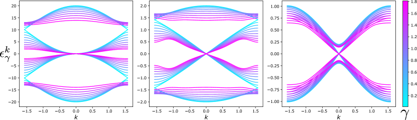
Figure 2: Dispersions $\pm\epsilon_{\gamma}^{k}$ for $\mathbf{H_{\gamma}}$. From the left: $\alpha=0.1,1,10$.

The spectrum turns out to be gapless for $k\to 0$, since

$$(\nu_{0}+\nu_{1})^{2}=\sum_{j=0}^{6}\mu_{j}=\frac{16}{\alpha^{4}\cosh^{4}\left(\frac{\gamma}{2}\right)}.$$ (3.12)

This implies that $\mathbf{H_{\gamma}}$ is critical for all $\gamma$ and that topological phases are only possible if the global fermionic symmetry is broken.

To make this explicit, we zoom in on $k=0$, where the hamiltonian $\mathbf{H_{\gamma}}$ reduces to two $2\times 2$ blocks on the bases $\mathbf{M}=\{\ket{-},\ket{0,\pi}\}$ and $\mathbf{N}=\{\ket{0},\ket{\pi}\}$,

$$\mathbf{H_{\gamma}^{0,M}}=\left(\begin{matrix}-\frac{N_{1}^{0}+N_{2}^{0}}{2}&0\\ 0&\frac{N_{1}^{0}+N_{2}^{0}}{2}\end{matrix}\right), \mathbf{H_{\gamma}^{0,N}}=\left(\begin{matrix}\frac{N_{1}^{0}-N_{2}^{0}}{2}&H^{0}\\ H^{0}&\frac{-N_{1}^{0}+N_{2}^{0}}{2}\end{matrix}\right).$$ (3.13)

with the superscript 0 denoting the value for $k=0$. Using that

$$N_{1}^{0}=-\frac{2}{\alpha}\frac{\sinh^{2}(\frac{\gamma}{4})}{\cosh^{2}(\frac{\gamma}{2})},\quad N_{2}^{0}=-\frac{2}{\alpha}\frac{\cosh^{2}(\frac{\gamma}{4})}{\cosh^{2}(\frac{\gamma}{2})},\quad H^{0}=\sqrt{N_{1}^{0}N_{2}^{0}},$$ (3.14)

it is found that both these blocks give energies $\pm(N_{1}^{0}+N_{2}^{0})/2$ and we conclude that the 1-particle (BdG) energies are

$$(\epsilon_{\gamma}^{k=0})_{1}=0,\quad(\epsilon_{\gamma}^{k=0})_{2}=-N_{1}^{0}-N_{2}^{0}=\frac{2}{\alpha}\frac{1}{\cosh(\frac{\gamma}{2})}\ .$$ (3.15)

The 1-particle zero-mode going with $(\epsilon^{k=0}_{\gamma})_{1}=0$ is found to be

$$(\eta_{\gamma}^{k=0})_{1}=\sqrt{\frac{-1}{N_{1}^{0}+N_{2}^{0}}}\left(\sqrt{-N_{2}^{0}}c_{0}-\sqrt{-N_{1}^{0}}c_{\pi}\right)=\frac{1}{2\sqrt{L}}\frac{1}{\cosh(\frac{\gamma}{2})}\left(Q^{L}(\gamma,0)-iQ^{R}(\gamma,0)\right).$$ (3.16)

This makes explicit that the global fermionic charges constitute a zero mode of $\mathbf{H_{\gamma}}$ and that both $Q^{L}(\gamma,0)$ and $Q^{R}(\gamma,0)$ commute with $\mathbf{H_{\gamma}}$.

In the limit $\gamma\to 0$, where translational symmetry is restored, the model reduces to the critical Kitaev chain. This is shown in figure 3. The model exhibits 4 distinct bands that collapse into 2 in the limit $\gamma\to 0$.

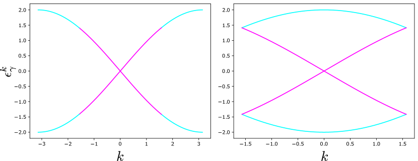
Figure 3: Folding of the Brillouin Zone of hamiltonian B.1 for $\alpha=1$, $\gamma=0$. From the left: $-\pi<k<\pi$, $-\pi/2<k<\pi/2$.

3.3 $\gamma\neq 0$ - Symmetry breaking and topological phases

To study the topological properties of the model it is convenient to write the hamiltonian Bogoliubov-de Gennes (BdG) form,

$$\mathbf{H_{\gamma}}=\frac{1}{2}\sum_{k}\Psi_{k}^{\dagger}\Lambda_{k}\Psi_{k}\,,$$ (3.17)

with Nambu spinors and local hamiltonian

$$\Psi=\left(\begin{matrix}c_{k}\\ c_{k-\pi}\\ c_{-k}^{\dagger}\\ c_{\pi-k}^{\dagger}\end{matrix}\right)\,, \Lambda_{k}=\left(\begin{matrix}N_{1}&H&S_{1}&S_{2}\\ H^{*}&N_{2}&S_{2}^{*}&-S_{1}\\ S_{1}&S_{2}&-N_{1}&-H\\ S_{2}^{*}&-S_{1}&-H^{*}&-N_{2}\end{matrix}\right)\,.$$ (3.18)

The explicit values of the coefficient can be found in appendix B.

Once a model is written in BdG form, it naturally exhibits particle-hole symmetry. The symmetry operator is then $\mathcal{P}=U_{\mathcal{P}}\mathcal{K}$, where $\mathcal{K}$ is the complex conjugation operator and $U_{\mathcal{P}}=\sigma^{x}\otimes\mathbb{1}$. It can be checked that $U_{\mathcal{P}}\Lambda_{k}^{*}U_{\mathcal{P}}^{\dagger}=-\Lambda_{-k}$. By looking at the coefficients of the hamiltonian it might seem that time reversal symmetry is absent, since some have complex values, but that is not the case. The time reversal operator turns out to be $\mathcal{T}=U_{\mathcal{T}}\mathcal{K}$, with $U_{\mathcal{T}}=i\sigma^{z}\otimes\mathbb{1}$, again the symmetry relation can be checked $U_{\mathcal{T}}\Lambda_{k}^{*}U_{\mathcal{T}}^{\dagger}=\Lambda_{-k}$. We point out that this representation of $\mathcal{T}$ is induced by our conventions yielding a purely imaginary coefficient $\Delta=ib_{12}$ of the superconducting pairing term, see eq. 2.22. The connection with the usual representation for real $\Delta$, $\mathcal{T}=\mathcal{K}$, can be established through conjugation of $\mathcal{T},\mathcal{P}$ under the transformation $G=e^{i\frac{\pi}{4}(\sigma^{z}\otimes\mathbb{1})}$. Given that both time reversal and particle hole symmetry are present the hamiltonian also exhibits a chiral symmetry with $\mathcal{C}=U_{\mathcal{C}}=U_{\mathcal{P}}U_{\mathcal{T}}$ and $U_{\mathcal{C}}\Lambda_{k}U_{\mathcal{C}}^{\dagger}=-\Lambda_{k}$. Since all three symmetry operators square to the identity, $\mathcal{P}^{2}=\mathcal{T}^{2}=\mathcal{C}^{2}=\mathbb{1}$, the model is in the topological insulator class BDI. Moreover, we point out the absence of sublattice symmetry, caused by the presence of chemical potentials entering as diagonal terms in the representation of our hamiltonian $\Lambda_{k}$. This implies the non-existence of SSH-like phases for our model.

In $d=1$ the BDI class is characterized by a $\mathbb{Z}$ index. Given the symmetries of the model and the absence of SSH-like phases, which would manifest through localized fermionic zero-modes, we can only expect the presence of Majorana zero-modes (MZM). In order to probe this, we employ the chiral index [22], whose absolute value quantifies the number of MZM which would localize at each end of an OBC instance of the system. With a unitary rotation we can transform the local hamiltonian into an off-diagonal operator,

$$U_{\mathcal{M}}=\frac{1}{2}\left(\begin{matrix}1+i&0&1-i&0\\ 0&1+i&0&1-i\\ 1+i&0&-1+i&0\\ 0&1+i&0&-1+i\\ \end{matrix}\right) U_{\mathcal{M}}\Lambda_{k}U_{\mathcal{M}}^{\dagger}=\left(\begin{matrix}0&V(k)\\ V^{\dagger}(k)&0\end{matrix}\right)\,.$$ (3.19)

Our unitary transformation $U_{\mathcal{M}}$ is related to the usual rotation $U=e^{-i\frac{\pi}{4}(\sigma^{y}\otimes\mathbb{1})}$ taking a BdG hamiltonian with real $\Delta$ to a purely off-diagonal form (cf. [22]) through $G$, as $U_{\mathcal{M}}=UG$. By a redefinition of the rotation $U$ by conjugation under $G$, $V=G^{\dagger}UG$, one gets:

$$V\Lambda_{k}V^{\dagger}=\left(\begin{matrix}0&-iV(k)\\ iV^{\dagger}(k)&0\end{matrix}\right)\,.$$ (3.20)

Finally, defining the complex function $z(k)=\det[V(k)]/|\det[V(k)]|=\exp[i\psi(k)]$, the winding number is:

$$W=\frac{1}{2\pi i}\int_{-\frac{\pi}{2}}^{\frac{\pi}{2}}\frac{dz(k)}{z(k)}=\frac{1}{2\pi i}\operatorname{Tr}\int_{-\frac{\pi}{2}}^{\frac{\pi}{2}}dk\,V^{-1}(k)\partial_{k}V(k).$$ (3.21)

The winding number can be explicitly calculated by computing the integral above for an arbitrary choice of the parameters $\alpha$ and $\gamma$; as long as our global fermionic symmetry is in place, numerical evidence shows that $W=0$. Therefore the hamiltonian $\mathbf{H_{\gamma}}$ describes a topologically trivial model, in agreement with our earlier observation that $\mathbf{H_{\gamma}}$ is always gapless.

In order to access non-trivial phases we perturb the system such that $\mathcal{C}$, $\mathcal{P}$ and $\mathcal{T}$ symmetries, as well as the free-fermionic nature of the model, are retained, but the global fermionic symmetry is broken. This approach stems from the interpretation of the fermionic symmetry as the responsible for the impossibility to move away from criticality through a change of parameters. In principle, one could choose to perturb directly the UBW generating $\mathbf{H_{\gamma}}$ through a modification of the coefficients in 2.20. That would also allow to exit the global fermionic symmetry submanifold, resulting in non-trivial topological phases. Our choice is to extract the hamiltonian limit from the UBW and then perturb its BdG form directly, leaving the other analysis for future work. We do it in the following way:

$$J_{AB}^{L}\to J_{AB}^{L}+\delta N_{A}\to N_{A}+\epsilon_{1} N_{B}\to N_{B}+\epsilon_{2}.$$ (3.22)

Now we can calculate the winding number for fixed values of $\alpha$ and $\gamma$, while changing the strength of the perturbations. As mentioned above, the absolute value of the index $W$ quantifies the number of MZM which can localize at each end of an open chain. Figures 4-4 show how we are able to access the Kitaev-like phase ($|W|=1$), which implies localization of a MZM at each end of an OBC instance of the system. In the $\gamma=0$ limit, shown in fig. 4, we see how perturbing the chemical potential $\epsilon$ as we keep $\delta=0$ is equivalent to satisfying the condition $|\mu|<2|t|$ to achieve the non-trivial topological phase of the Kitaev chain. For $\delta\neq 0$, we observe how the condition is always met in this parameter range as far as $\epsilon<\delta$. We also point out the absence of gap-closing lines corresponding to the boundaries of the $W=1$ phase in figure 4. This happens because the $W=\pm 1$ phases differ by a global phase factor and are thus equivalent.

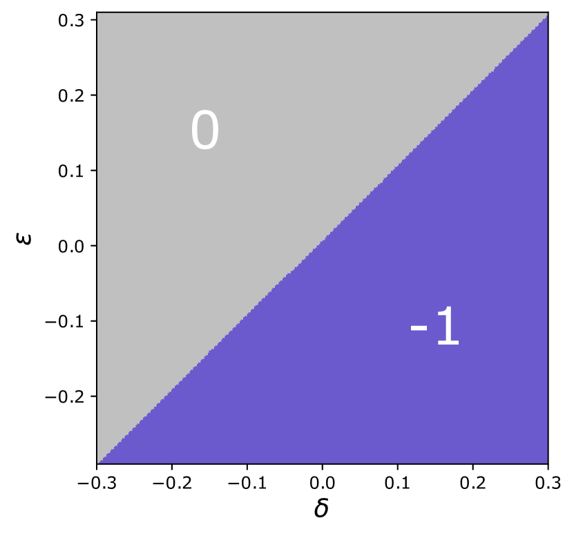
(a) $\alpha=1,\gamma=0,\epsilon_{1}=\epsilon_{2}$

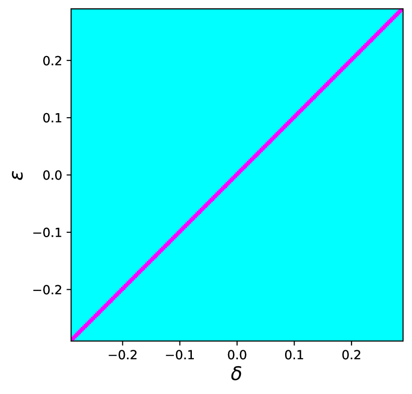
(b)

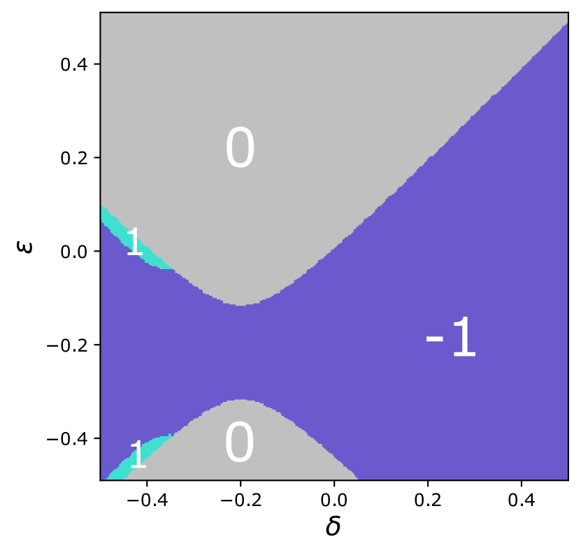
(c) $\alpha=5,\gamma=1,\epsilon_{1}=\epsilon_{2}$

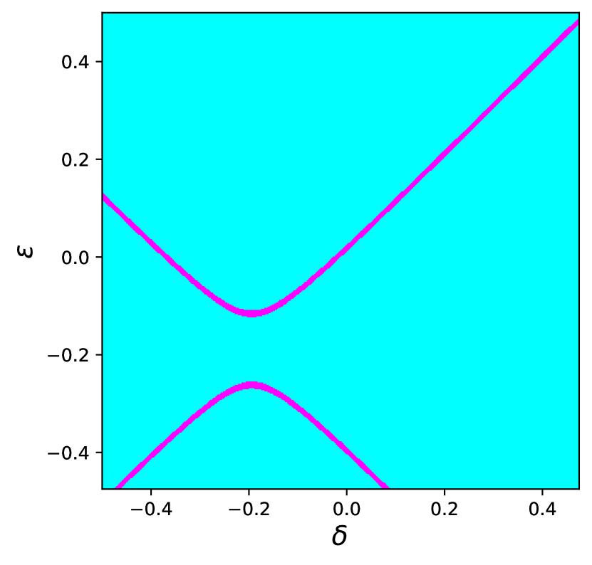
(d)

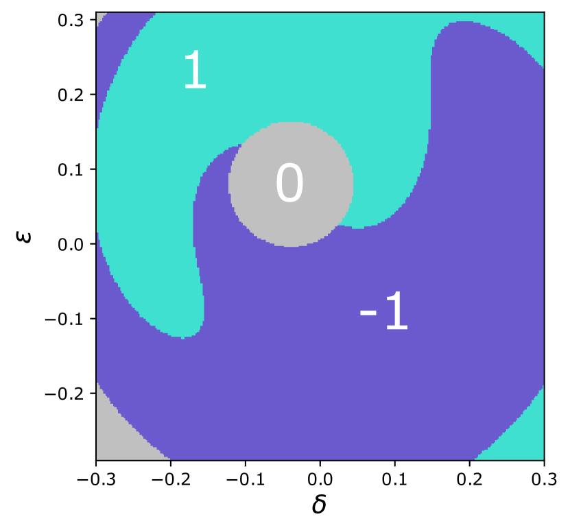
(e) $\alpha=5,\gamma=3,\epsilon_{1}=-\epsilon_{2}$

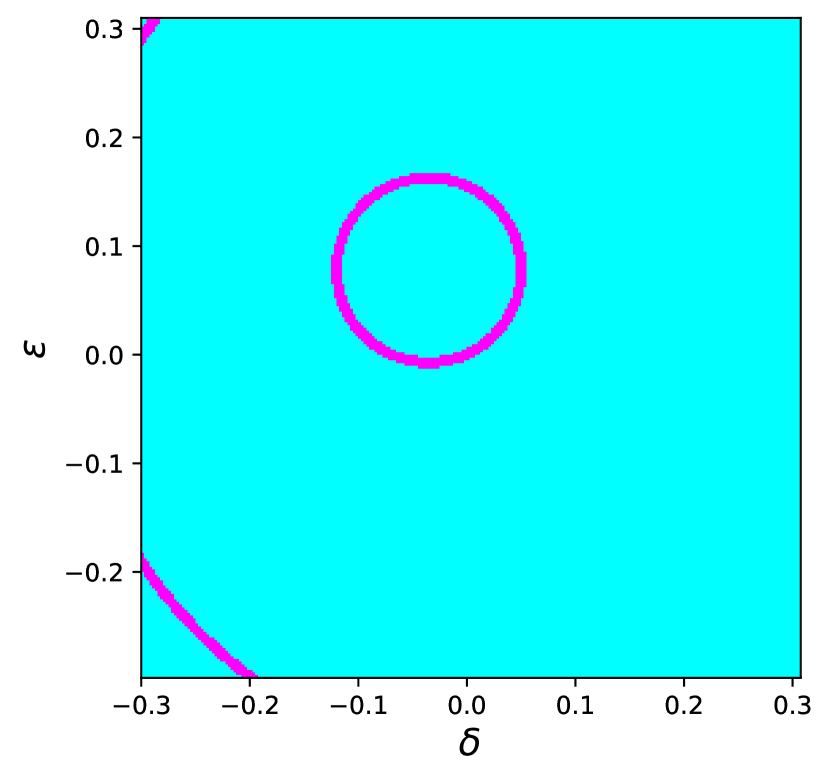
(f)

Figure 4: Topological phase diagrams for the chiral index $W$ (left) and energy gap-closing points (right) as functions of $\epsilon$ and $\delta$.

4 Brick wall circuits: spectral analysis

We now turn to the spectral analysis of the full UBW operator $\mathbf{U_{F}}(\alpha,\gamma,\theta)$. For $\gamma=0$, the results will reduce to those for the hamiltonian $\mathbf{H_{0}}(\alpha)$ in the limit where $\theta\to 0$. For $\gamma\neq 0$ such a direct connection does not exist.

Our analysis will lead to (somewhat implicit) expressions for the 1-particle dispersion relations $\epsilon_{i}^{k}$. We anticipate that the global fermionic symmetry that we built into the UBW circuit will force one of the $\epsilon_{i}^{k}$ to approach 0 in the limit $k\to 0$, causing a degeneracy in the (logarithmic) spectrum of $\mathbf{U_{F}}(\alpha,\gamma,\theta)$. Surprisingly, other gapless points arise as well and upon fine-tuning $\theta=\pm\gamma$ we see a coalescence that leads to a cubic dispersion $\epsilon^{k}\propto k^{3}$.

4.1 Structure of UBW in momentum space

We consider the general UBW $\mathbf{U_{F}}(\alpha,\gamma,\theta)$ on (an even number of) $L$ sites and with periodic boundary conditions (PBC), see fig. 5. The two sublayers making up $\mathbf{U_{F}}(\alpha,\gamma,\theta)$ are expressed as

$$\mathbf{U_{o}}=\exp[i\mathbf{E_{o}}]=\exp\left[i\sum_{i=1}^{L/2}\mathbf{E}_{2i,2i+1}\right],\qquad\mathbf{U_{e}}=\exp[i\mathbf{E_{e}}]=\exp\left[i\sum_{i=1}^{L/2}\mathbf{E}_{2i-1,2i}\right].$$ (4.1)

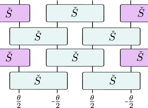
Figure 5: General brick wall circuit with periodic boundary conditions

We will proceed by writing each layer in momentum space. The explicit breaking of translation symmetry between the even and odd sites causes a reduction of the Brillouin zone to to $-\pi/2<k\leq\pi/2$. The symmetry $k\to-k$ gives a further reduction and we can analyze the spectral structure restricting to momenta $0\leq k\leq\pi/2$.

For general $k$, the action of the $\mathbf{E}_{i,i+1}$ will mix the 1-fermi operators with momentum $k$, $-k$, $\pi-k$ and $k-\pi$ and we will have to handle the action of the $\mathbf{E}_{i,i+1}$ on the span of the these operators, which in general has dimension 16. We first consider the simpler sectors where $k=0$ or $k=\pi/2$.

4.2 Spectral analysis for $k=0$ and $k=\pi/2$

For the sector with $k=0,\pi$ the momentum space exponents read

$$\mathbf{E_{o}^{0}} = -a_{11}\left(c_{0}^{\dagger}c_{0}+c_{\pi}^{\dagger}c_{\pi}-1\right)+ib_{12}\left(c_{0}^{\dagger}c_{\pi}^{\dagger}-c_{\pi}c_{0}\right)$$ (4.2)

$$+a_{12}\cos(\phi)\left(c_{0}^{\dagger}c_{0}-c_{\pi}^{\dagger}c_{\pi}\right)-ia_{12}\sin(\phi)\left(c_{0}^{\dagger}c_{\pi}-c_{\pi}^{\dagger}c_{0}\right)$$

and

$$\mathbf{E_{e}^{0}} = -a_{11}\left(c_{0}^{\dagger}c_{0}+c_{\pi}^{\dagger}c_{\pi}-1\right)-ib_{12}\left(c_{0}^{\dagger}c_{\pi}^{\dagger}-c_{\pi}c_{0}\right)$$ (4.3)

$$+a_{12}\cos(\phi)\left(c_{0}^{\dagger}c_{0}-c_{\pi}^{\dagger}c_{\pi}\right)+ia_{12}\sin(\phi)\left(c_{0}^{\dagger}c_{\pi}-c_{\pi}^{\dagger}c_{0}\right)\ .$$

This gives rise to two $2\times 2$ blocks for the exponents in matrix form. On the basis $\{\ket{-},\ket{0,\pi}\}$ these are

$$\mathbf{E_{o}^{0,M}}=\left(\begin{matrix}a_{11}&-ib_{12}\\ +ib_{12}&-a_{11}\end{matrix}\right),\quad\mathbf{E_{e}^{0,M}}=\left(\begin{matrix}a_{11}&ib_{12}\\ -ib_{12}&-a_{11}\end{matrix}\right),$$ (4.4)

and on basis $\{\ket{0},\ket{\pi}\}$

$$\mathbf{E_{o}^{0,N}}=a_{12}\left(\begin{matrix}\cos\phi&-i\sin\phi\\ i\sin\phi&-\cos\phi\end{matrix}\right),\quad\mathbf{E_{e}^{0,N}}=a_{12}\left(\begin{matrix}\cos\phi&i\sin\phi\\ -i\sin\phi&-\cos\phi\end{matrix}\right).$$ (4.5)

It is an elementary exercise to exponentiate and then multiply these matrices and to extract the characteristic polynomial $\mathbf{Char^{0}}(x)=\prod(\lambda_{i}-x)$ of $\mathbf{U_{F}^{0}}(\alpha,\gamma,\theta)$ in both these sectors.

Specializing to $a_{11}$, $a_{12}$, $\phi$ and $b_{12}$ as given in eq. 2.20, we obtain, in both the $M$ and the $N$ sectors,

$$\mathbf{Char^{0}}(x)=x^{2}-2\frac{2\alpha^{2}(\cosh(\gamma)+\cosh(\theta))-\sinh(\theta)^{2}}{2\alpha^{2}(\cosh(\gamma)+\cosh(\theta))+\sinh(\theta)^{2}}x+1$$ (4.6)

Clearly, the global fermionic symmetry maps between the two sectors and causes the eigenvalues to be identical between the two. Unitarity and particle-hole symmetry guarantee that the eigenvalues come in a pair $\{\lambda,\lambda^{*}\}$ with $|\lambda|=1$.

Translating to 1-particle energies, we find

$$\epsilon_{1}^{k=0}=0,\qquad\epsilon_{2}^{k=0}=2\arccos\left(\frac{2\alpha^{2}(\cosh(\gamma)+\cosh(\theta))-\sinh^{2}(\theta)}{2\alpha^{2}(\cosh(\gamma)+\cosh(\theta))+\sinh^{2}(\theta)}\right)$$ (4.7)

and we have $\mathbf{U_{F}^{0}}(\alpha,\gamma,\theta)=\exp[\sum_{i}\epsilon_{i}^{k=0}(\eta^{\dagger}_{i}\eta_{i}-\frac{1}{2})]$. The 1-particle operators for the zero-energy mode are given by linear combinations of the two fermionic charges,

$$\eta^{k=0}_{1}=\frac{1}{2\sqrt{L}}\left(\frac{\mathbf{Q^{L}}(\gamma,\theta)}{\sqrt{\cosh(\frac{\gamma+\theta}{2}})}-i\frac{\mathbf{Q^{R}}(\gamma,\theta)}{\sqrt{\cosh(\frac{\gamma-\theta}{2})}}\right).$$ (4.8)

Repeating the analysis for the sector with $k=\frac{\pi}{2}$ and $k=-\frac{\pi}{2}$, we find on basis $\{\ket{-},\ket{\frac{\pi}{2},-\frac{\pi}{2}}\}$

$$\mathbf{E^{\pi/2,M}_{o}}=\left(\begin{matrix}a_{11}&-b_{12}\\ -b_{12}&-a_{11}\end{matrix}\right),\quad\mathbf{E^{\pi/2,M}_{e}}=\left(\begin{matrix}a_{11}&-b_{12}\\ -b_{12}&-a_{11}\end{matrix}\right)$$ (4.9)

and on basis $\{\ket{\frac{\pi}{2}},\ket{-\frac{\pi}{2}}\}$

$$\mathbf{E^{\pi/2,N}_{o}}=a_{12}\left(\begin{matrix}\sin\phi&i\cos\phi\\ -i\cos\phi&-\sin\phi\end{matrix}\right)\quad\mathbf{E^{\pi/2,N}_{e}}=a_{12}\left(\begin{matrix}\sin\phi&-i\cos\phi\\ i\cos\phi&-\sin\phi\end{matrix}\right).$$ (4.10)

This leads to

$$\mathbf{Char^{\pi/2,N}}(x)=x^{2}-2\left(2-\frac{8\alpha^{2}(\cosh(\gamma)-1)}{2\alpha^{2}(\cosh(\gamma)+\cosh(\theta))+\sinh^{2}(\theta)}\right)x+1$$ (4.11)

and

$$\mathbf{Char^{\pi/2,M}}(x)=x^{2}-2\left(-2+\frac{8\alpha^{2}(\cosh(\gamma)+1)}{2\alpha^{2}(\cosh(\gamma)+\cosh(\theta))+\sinh^{2}(\theta)}\right)x+1.$$ (4.12)

In this case the 1-particle energies are both non-zero in general. However, one of the 1-particle energies $\epsilon_{i}^{k=\pi/2}$ vanishes when the sectors $\mathbf{M}$, $\mathbf{N}$ give identical eigenvalues, which happens for

$$2\alpha^{2}\big{(}\cosh(\gamma)-\cosh(\theta)\big{)}=\sinh^{2}(\theta).$$ (4.13)

4.3 Spectral analysis for general k

For fixed $k$ satisfying $0<k<\pi/2$ we find the following expressions

$$\begin{split}\mathbf{E^{k}_{o,e}}=&\left\{-a_{11}\left(c_{k}^{\dagger}c_{k}+c_{-k}^{\dagger}c_{-k}+c_{k-\pi}^{\dagger}c_{k-\pi}+c_{\pi-k}^{\dagger}c_{\pi-k}-2\right)\right.\\ &\hskip 28.45274pt+a_{12}\cos(k-\phi)\left(c_{k}^{\dagger}c_{k}-c_{k-\pi}^{\dagger}c_{k-\pi}\right)\\ &\hskip 28.45274pt+a_{12}\cos(k+\phi)\left(c_{-k}^{\dagger}c_{-k}-c_{\pi-k}^{\dagger}c_{\pi-k}\right)\\ &\hskip 28.45274pt\pm ia_{12}\sin(k-\phi)\left(c_{k}^{\dagger}c_{k-\pi}-c_{k-\pi}^{\dagger}c_{k}\right)\\ &\hskip 28.45274pt\pm ia_{12}\sin(k+\phi)\left(c_{\pi-k}^{\dagger}c_{-k}-c_{-k}^{\dagger}c_{\pi-k}\right)\\ &\hskip 28.45274pt\mp ib_{12}\cos(k)\left(c_{k}^{\dagger}c_{\pi-k}^{\dagger}-c_{\pi-k}c_{k}+c_{-k}^{\dagger}c_{k-\pi}^{\dagger}-c_{k-\pi}c_{-k}\right)\\ &\hskip 28.45274pt\left.+b_{12}\sin(k)\left(c_{k}^{\dagger}c_{-k}^{\dagger}+c_{-k}c_{k}+c_{\pi-k}^{\dagger}c_{k-\pi}^{\dagger}+c_{k-\pi}c_{\pi-k}\right)\right\}\end{split}$$ (4.14)

with the top (bottom) sign referring to the odd (even) layer.

The block structure for given $k$ is similar to that for $\mathbf{H_{\gamma}}$, described in section 3.2. The exponents $\mathbf{E^{k}_{o}}$ and $\mathbf{E^{k}_{e}}$ decompose in blocks of dimension 1, 4, 6, 4, 1. The corresponding bases are

1. M₁: $\{\ket{k,k+\pi}\}$ and M${}^{\prime}_{1}$: $\{\ket{-k,-k+\pi}\}$. On both these states both the even and odd exponents act trivially, meaning these states are inert under the UBW operator,

2. M₆: $\{\ket{-},\ket{k,-k},\ket{k,-k+\pi},\ket{k+\pi,-k},\ket{k+\pi,-k+\pi},\ket{k,k+\pi,-k,-k+\pi}\}$,

3. N₄: $\{\ket{k},\ket{k+\pi},\ket{k,k+\pi,-k},\ket{k,k+\pi,-k+\pi}\}$,

4. N${}^{\prime}_{4}$: $\{\ket{-k},\ket{-k+\pi},\ket{-k,-k+\pi,k},\ket{-k,-k+\pi,k+\pi}\}$.

The unitary brick wall (UBW) operator in this sector takes the form

$$\mathbf{U_{F}^{k}}(\alpha,\gamma,\theta)=\exp\left[i\sum_{i}\epsilon_{i}^{k}(\eta^{k\,\dagger}_{i}\eta^{k}_{i}-{\frac{1}{2}})\right].$$ (4.15)

This implies that the 16 eigenvalues in the sector labeled with $k$ are products of four factors of the form $\lambda_{i}=\exp(i\epsilon^{k}_{i})$ or $\lambda^{*}_{i}=\exp(-i\epsilon^{k}_{i})$, $i=1,2,3,4$. Knowing that the states M₁ and M${}^{\prime}_{1}$ have zero energy we conclude that some linear combination of the energies $\epsilon_{i}$ vanishes, say $\pm(\epsilon_{1}+\epsilon_{2}+\epsilon_{3}+\epsilon_{4})=0$. In fact, for $\gamma=0$ we have $\epsilon_{1}+\epsilon_{3}=0$ and $\epsilon_{2}+\epsilon_{4}=0$.

Clearly, the states in the sector N₄ and N${}^{\prime}_{4}$ are related to the state M₁ by a single creation or annihilation operator, hence a single operator $\eta^{\dagger}_{i}$. The single particle energies $\epsilon_{i}$ are thus found by diagonalizing N₄ and N${}^{\prime}_{4}$. The characteristic polynomial of $\mathbf{U_{F}^{k}}$ on the basis N₄ takes the form

$$\mathbf{Char^{k,N_{4}}}(x) =(x-\lambda_{1})(x-\lambda_{2})(x-\lambda_{3})(x-\lambda_{4})$$

$$=(x-\lambda_{1})(x-\lambda_{2})(x-\lambda_{3})(x-\lambda^{*}_{1}\lambda^{*}_{2}\lambda^{*}_{3})$$ (4.16)

and it will thus be of the general form

$$\mathbf{Char^{k,N_{4}}}(x)=x^{4}-a_{4}x^{3}+b_{4}x^{2}-a^{*}_{4}x+1.$$ (4.17)

The other $4\times 4$ block will have a similar form but with the conjugate coefficients.

$$\mathbf{Char^{k,N^{\prime}_{4}}}(x)=x^{4}-a^{*}_{4}x^{3}+b_{4}x^{2}-a_{4}x+1.$$ (4.18)

Clearly, via all definitions made in the above, the coefficients $a_{4}$, $b_{4}$ can be expressed in the parameters $\alpha$, $\gamma$ and $\theta$ of the defining 2-qubit gate $\mathbf{\check{S}}(\alpha,\gamma,\theta)$ but the derivation of these expressions is quite cumbersome. In the most general case the two coefficients are

$$\begin{split}a_{4}&=\frac{1}{2\left(2\alpha^{2}(\cosh(\gamma)+\cosh(\theta))+\sinh^{2}(\theta)\right)^{2}}\\ &\qquad\times\Big{(}8\alpha^{2}\big{[}8\alpha^{2}\cosh(\gamma)\cosh(\theta)+8\alpha^{2}+\cosh(\theta)-\cosh(3\theta)\big{]}\\ &\qquad\qquad+\big{[}16\alpha^{4}(\cosh(2\gamma)+\cosh(2\theta))-32\alpha^{4}-32\alpha^{2}\cosh(\gamma)\sinh^{2}(\theta)\\ &\qquad\qquad\qquad-4\cosh(2\theta)+\cosh(4\theta)+3\big{]}\cos(2k)\\ &\qquad\qquad-64\,i\,\alpha^{2}\sinh(\gamma)\sinh^{2}(\theta)\sin(2k)\Big{)},\end{split}$$ (4.19)

$$\begin{split}b_{4}&=\frac{1}{2\left(2\alpha^{2}(\cosh(\gamma)+\cosh(\theta))+\sinh^{2}(\theta)\right)^{2}}\\ &\qquad\times\Big{(}16\alpha^{4}(\cosh(2\gamma)+\cosh(2\theta))+160\alpha^{4}-96\alpha^{2}\cosh(\gamma)\sinh^{2}(\theta)\\ &\qquad\qquad-4\cosh(2\theta)+\cosh(4\theta)+3\\ &\qquad\qquad+64\alpha^{2}\big{[}-2\alpha^{2}+\cosh(\theta)(2\alpha^{2}\cosh(2\gamma)-\sinh^{2}(\theta))\big{]}\cos(2k)\\ &\qquad\qquad+\big{[}4\alpha^{2}(\cosh(\gamma)-\cosh(\theta))+2\sinh^{2}(\theta)\big{]}^{2}\cos(4k)\,\Big{)}.\end{split}$$ (4.20)

A useful check is that in the limit $k\to 0$ the solutions to $\mathbf{Char^{k,N_{4}}}(x)=0$ reduce to $\exp[\pm i\epsilon_{1}^{k=0}]=1$ and $\exp[\pm i\epsilon_{2}^{k=0}]$. Another check is that $a_{4}=4$ and $b_{4}=6$ in the limit $\gamma,\,\theta\to 0$, as all eigenvalues reduce to 1 in that limit.

In the general case, where $a^{*}_{4}\neq a_{4}$, solving for $\lambda_{i}^{k}$ requires solving a quartic equation. However, we observe that the numbers $c_{12}=\cos(\epsilon^{k}_{1}+\epsilon^{k}_{2})$, $c_{13}=\cos(\epsilon^{k}_{1}+\epsilon^{k}_{3})$ and $c_{23}=\cos(\epsilon^{k}_{2}+\epsilon^{k}_{3})$ satisfy

$$c_{12}+c_{13}+c_{23}=\frac{b_{4}}{2},\quad c_{12}c_{13}+c_{12}c_{23}+c_{13}c_{23}=\frac{a_{4}a_{4}^{*}-4}{4},\quad c_{12}c_{13}c_{23}=\frac{a_{4}^{2}+(a_{4}^{*})^{2}-4b_{4}}{8}.$$

This implies that the $c_{ij}$ can be expressed as the roots of a third order polynomial, giving closed-form but involved expressions for the $\epsilon^{k}_{i}$.

In the following subsections we briefly report on the special limits where $\gamma=0$ (equal masses) or $\gamma=\theta$.

4.3.1 Equal masses

First the case with equal masses, $\gamma=0$, so that also $\phi=0$. In this case $\mathbf{Char^{k,N_{4}}}(x)=\mathbf{Char^{k,N^{\prime}_{4}}}(x)$, $a_{4}$ is real and the expressions for $a_{4}$ and $b_{4}$ reduce to

$$a_{4} =\frac{-1}{(-1+2\alpha^{2}+\cosh(\theta))^{2}}$$

$$\qquad\times\Big{(}\frac{4\alpha^{2}}{\cosh^{2}(\theta/2)}[1-4\alpha^{2}-2\cosh(\theta)+\cosh(2\theta)]$$

$$\qquad\qquad-2\tanh^{2}(\theta/2)[-1-8\alpha^{2}+8\alpha^{4}+\cosh(2\theta)]\,\cos(2k)\Big{)},$$ (4.21)

$$b_{4} =\frac{1}{(-1+2\alpha^{2}+\cosh(\theta))^{2}}$$

$$\qquad\times\Big{(}\frac{1}{8\cosh^{4}(\theta/2)}[3+48\alpha^{2}+176\alpha^{4}+4(-1+4\alpha^{2}(-3+\alpha^{2}))\cosh(2\theta)+\cosh(4\theta)]$$

$$\qquad\qquad-8\alpha^{2}\frac{\sinh^{2}(\theta/2)}{\cosh^{4}(\theta/2)}[1-4\alpha^{2}+2\cosh(\theta)+\cosh(2\theta)]\,\cos(2k)$$

$$\qquad\qquad+2\tanh^{4}(\theta/2)[1-2\alpha^{2}+\cosh^{2}(\theta)]^{2}\,\cos(4k)\Big{)}.$$ (4.22)

For $\gamma=0$ the cosines of the (logarithmic) energies $\epsilon^{k}_{i}$ can be expressed as

$$\cos(\epsilon^{k}_{1,2})=\frac{a_{4}}{4}\pm{\frac{1}{4}}\sqrt{a_{4}^{2}-4b_{4}+8}$$ (4.23)

bringing us as close as possible to a closed form expression.

4.3.2 The case $\gamma=\theta$

Note that in this case $a_{12}^{2}=a_{11}^{2}+b_{12}^{2}$. The coefficients of the characteristic polynomial of the UBW on basis N₄ now come out as

$$a_{4} =\frac{1}{(4\alpha^{2}\cosh(\theta)+\sinh^{2}(\theta))^{2}}$$

$$\qquad\times\Big{(}4\alpha^{2}(\cosh(\theta)+4\alpha^{2}(3+\cosh(2\theta))-\cosh(3\theta))$$

$$\qquad\qquad+2\sinh^{2}(\theta)(-1+16\alpha^{4}-8\alpha^{2}\cosh(\theta)+\cosh(2\theta))\,\cos(2k)$$

$$\qquad\qquad-32\,i\,\alpha^{2}\sinh^{3}(\theta)\sin(2k)\Big{)},$$ (4.24)

$$b_{4} =\frac{1}{2}\frac{1}{(4\alpha^{2}\cosh(\theta)+\sinh^{2}(\theta))^{2}}$$

$$\qquad\times\Big{(}3+160\alpha^{4}-4\cosh(2\theta)+8\alpha^{2}(3\cosh(\theta)+4\alpha^{2}\cosh(2\theta)-3\cosh(3\theta))$$

$$\qquad\qquad+\cosh(4\theta)-64\alpha^{2}(-2\alpha^{2}+\cosh(\theta))\sinh^{2}(\theta)\,\cos(2k)$$

$$\qquad\qquad+4\sinh^{4}(\theta)\cos(4k)\Big{)}.$$ (4.25)

Specializing to $k\to 0$, it is quickly checked that there are two solutions converging on $\epsilon=0$. Analyzing their dispersion, we find

$$\epsilon_{1}^{k\to 0}=-2\tanh(\theta)k+{\mathcal{O}}(k^{2}),\qquad\epsilon_{2}^{k\to 0}=\frac{\sinh(\theta)}{8\alpha^{2}}k^{3}+{\mathcal{O}}(k^{4}).$$

The cubic dispersion that we find here is unique to the choice $\theta=\pm\gamma$.

4.4 Dispersion relations for $\mathbf{U_{F}}$

We illustrate the spectral structure of $\mathbf{U_{F}}$ by showing some plots (figure 6,7,8) of the 1-particle dispersion $\pm\epsilon_{i}^{k}$, $i=1,\ldots,4$ and $k\in[0,\pi/2]$.

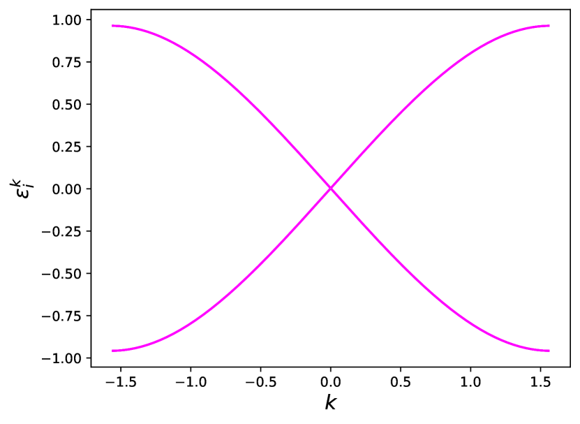
(a) $\alpha=1,\gamma=1,\theta=0$

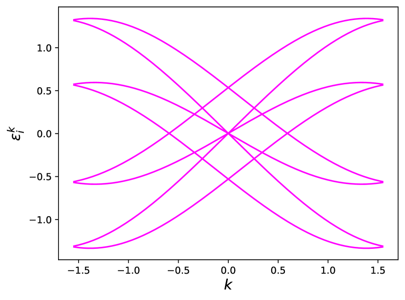
(b) $\alpha=1,\gamma=1,\theta=0.3$

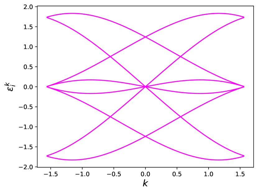
(c) $\alpha=1,\gamma=1,\theta=0.700(1)$

Figure 6: $\mathbf{U_{F}}$ spectrum for $\theta\leq\theta_{c}=0.700109$

As soon as $\theta>0$, there are two branches $\epsilon_{1}^{k}$ and $\epsilon_{2}^{k}$ that are gapless at $k=0$, while a third branch crosses zero at a finite $k$. For a critical value $\theta_{c}$ this finite $k$ reaches the value $k=\pi/2$. The critical value $\theta_{c}[\alpha,\gamma]$ is precisely the gapless point at $k=\pi/2$ that we identified in eq. 4.13. For $\alpha=1$, $\gamma=1$ we find $\theta_{c}=0.700109$.
Increasing $\theta$ beyond $\theta_{c}$, the values $\pm k$ giving a vanishing dispersion move towards $k=0$ and precisely for $\theta=\gamma$ they merge into a single multi-critical point with cubic dispersion, see eq. 4.3.2.

(a) $\alpha=1,\gamma=1,\theta=1$

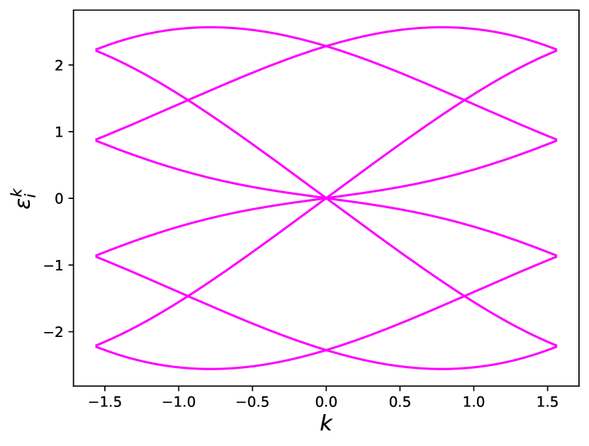
(b) $\alpha=1,\gamma=1,\theta=1.3$

Figure 7: $\mathbf{U_{F}}$ spectrum for $\theta\geq\theta_{c}$

We next consider these same dispersion plots for more general parameter choices which break the global fermionic symmetry. One way to break this symmetry is to scale the amplitude $a_{12}$ with a factor of $t_{a}$ with respect to the value, given in eq. 2.20, required by the fermionic symmetry. Clearly, reducing $t_{a}$ below $t_{a}=1$ is analogous to setting $2t<\mu$ in the Kitaev chain eq. 3.5 and one expects that a gap will open up.

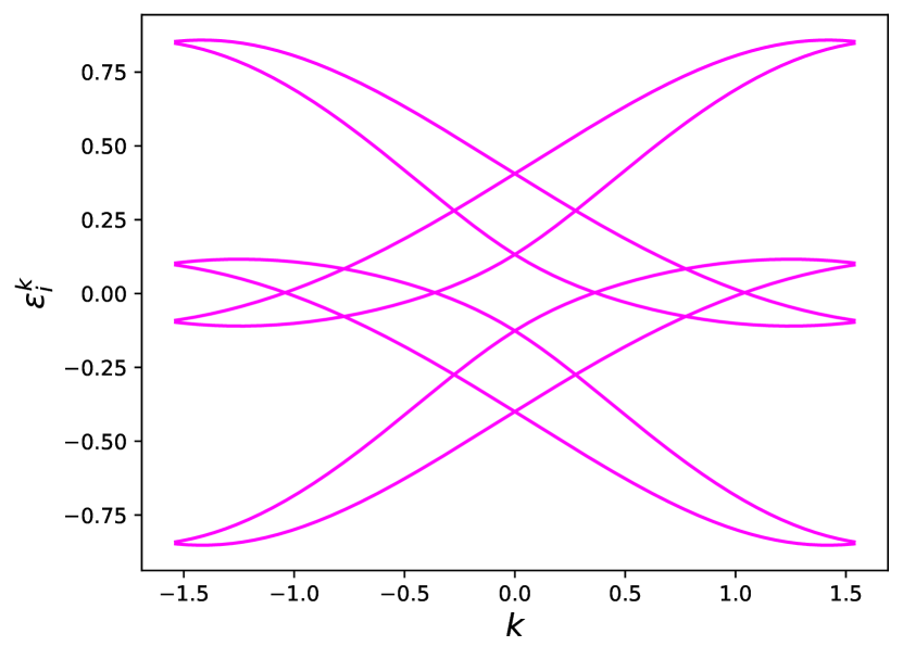
(a) $\alpha=1,\gamma=1,\theta=0.3,t_{a}=0.5$

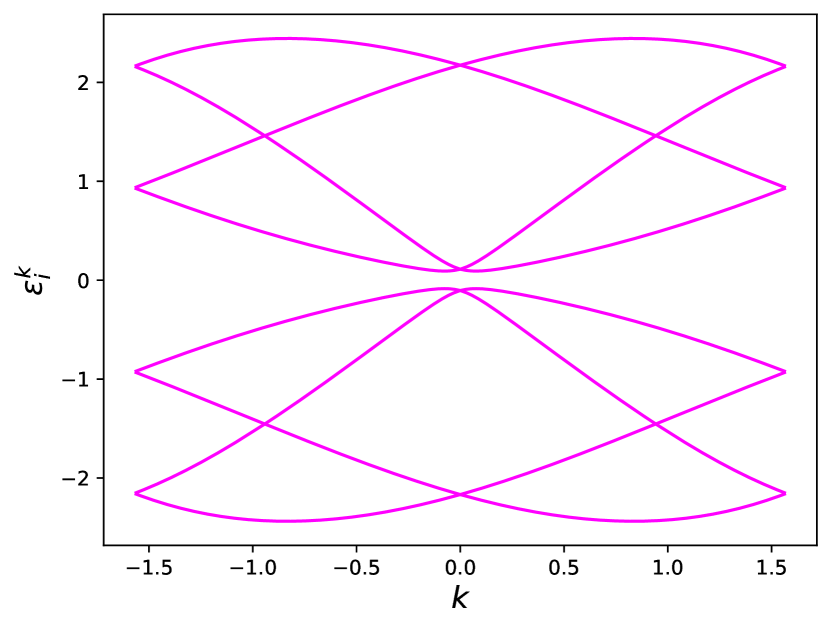
(b) $\alpha=1,\gamma=1,\theta=1.3,t_{a}=0.9$

Figure 8: $\mathbf{U_{F}}$ spectrum without global fermionic symmetry

Inspecting the behavior, we see that, for $\theta<\theta_{c}$ both the perturbations $t_{a}<1$ and $t_{a}>1$ move the gapless points away from $k=0$, but do not open a gap for all $k$. Only for $\theta\geq\theta_{c}$ and $t_{a}$ sufficiently below $t_{a}=1$ does an overall gap open up. Once $\theta\geq\gamma$, an arbitrary perturbation $\theta_{a}<1$ suffices to gap out all branches of the dispersion. This is also shown in figure 8. Changing the values of $\alpha$ and $\gamma$ gives a similar picture (as long as both remain non-zero). The critical value $\theta_{c}$ depends on both $\alpha$ and $\gamma$, while the point giving rise to a cubic dispersion is $\theta=\pm\gamma$ for all values of $\alpha$. We stress that the dispersion relations discussed in this section do not pertain to the hamiltonian $\mathbf{H_{\gamma}}$, but rather to the exponent $\mathbf{E}(\theta)$ characterizing the brick wall unitary $\mathbf{U_{F}}$ at finite values of $\theta$, see eq. 1.13.

5 Dynamics and entanglement entropy build up

Entanglement is a ubiquitous feature of quantum many-body systems. In the context of generic quantum simulations and quantum computations, a large amount of entanglement build-up during the system’s dynamical evolution is needed to achieve quantum advantage over classical simulation methods [27]. There exist exceptions, such as universal quantum computers operating with small entanglement generation, or highly entangled states which can be classically simulated [1, 2, 8, 24]. A widely used measure of entanglement is the Von Neumann entanglement entropy (EE). Given a density matrix $\rho$ and a bipartition $\{A,B\}$, the entanglement entropy for A is the Von Neumann entropy for the reduced density matrix of partition A, $\rho_{A}={\rm Tr}_{B}\rho$,

$$S_{A}=-{\rm Tr}[\rho_{A}\log(\rho_{A})].$$ (5.1)

A closely related quantity, which we will consider for our circuit analysis, is the second Rényi entropy (RE):

$$S^{(2)}_{A}=-{\rm Tr}[\log(\rho^{2}_{A})],$$ (5.2)

where $\rho^{2}_{A}$ is the purity of the quantum state.

All of the above motivates us to study the behaviour of entanglement in our model. We focus on the dynamical evolution of Rényi entropies of bipartitions $\{\{1,\ldots,L/2\},\{L/2+1,\ldots,L\}\}$ of the system after a global quench from different initial states, both with periodic and open boundary conditions (PBC/OBC), assigning the role of time to the spectral parameter $\theta$, for different choices of the interaction strength $\alpha$ and the mass ratio $\gamma$. For these numerical simulations we do not employ a Trotter scheme, as we just apply one layer of the UBW per $\theta$, fixing $\alpha$ and $\gamma$. A plot of the RE for different system sizes and PBC is given in figure 9(a). In the large-$\theta$ limit for this model the evolution operator reduces to a product of permutation matrices and RE($\theta$) goes to zero. On the other hand, for a 4-site system, we notice that for certain parameter choices we are able to reach maximally entangled states after a quench starting from the product state $|0\rangle^{\otimes L}$. One can consider figure 9(b), where the RE for the 4-site $\mathbf{U_{F}^{\rm OBC,extended}}$ (comprising of 4 layers to keep fermionic symmetry intact, see eq. 2.17) saturates to $2\log(2)$ for a certain range of $\theta$.

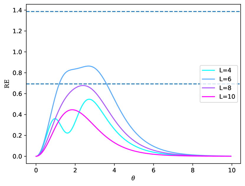
(a) RE for 1-layer PBC, $\alpha$=1, $\gamma$=1

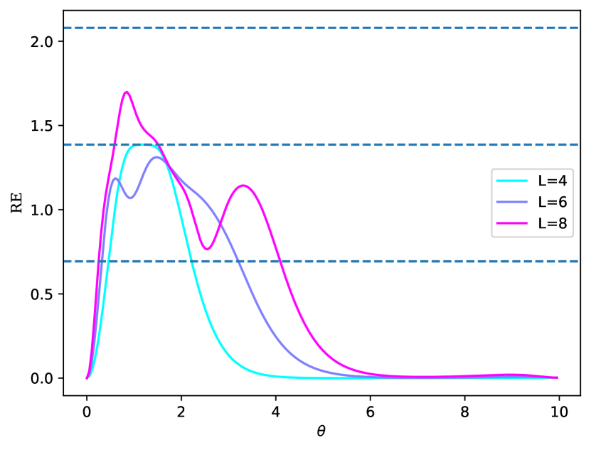
(b) RE for extended OBC, $\alpha$=1.2, $\gamma$=20

(c) RE for L=4 $m$-layer PBC, $\alpha$=0.15, $\gamma$=0

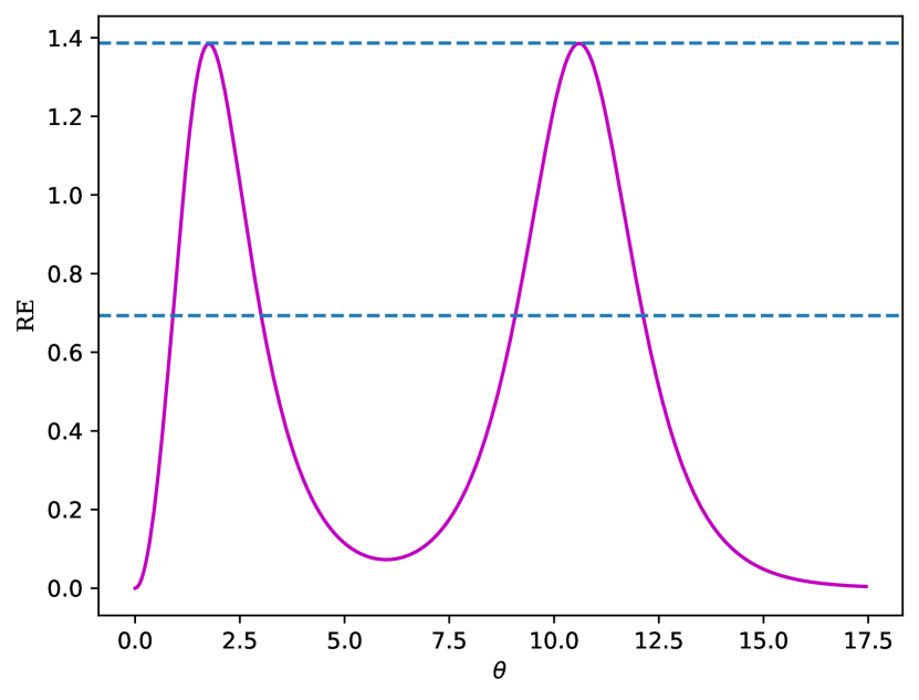
(d) RE for L=4 1-layer PBC, $\alpha$=100, $\gamma$=0

Figure 9: Rényi entropies for L=4 OBC/PBC circuits. All quenches are performed starting from the $|0\rangle^{\otimes L}$ state. Blue dashed lines represent multiples of $\log(2)$.

One can compute Rényi entropies for quenches from the all zero initial state under the evolution dictated by UBW. The unitary can be applied $m$ times per $\theta$, and in the $\alpha\ll 1$ regime, where non-linearities are less dominant, one can observe how the associated Rényi entropy will exhibit $m$ maxima. Let us first consider the case with a single layer per $\theta$. By direct inspection of the $L=4$ PBC circuit one can notice that the output state will present four dominant amplitudes, whereas the others will be equal to zero. A single layer of $\mathbf{U_{F}}^{\rm PBC}(\alpha,\gamma,\theta)$ yields

$$\mathbf{U_{F}}^{\rm PBC}(\alpha,\gamma,\theta)|0000\rangle$$ (5.3)

$$=\psi_{1}|0000\rangle+\psi_{2}(|0011\rangle+|1100\rangle)+\psi_{3}(|0110\rangle+|1001\rangle)+\psi_{4}|1111\rangle,$$

where $|\psi_{4}|\ll|\psi_{1,2,3}|$ and it can be neglected for all practical purposes. Following the arrow of time $\theta$ from the start of the quench, one notices that the amplitude of the $|0000\rangle$ state ($\psi_{1}$), which is initially set to one, exhibits one minimum associated to an increase in the (equal) amplitudes of Bell pairs $|0011\rangle+|1100\rangle$ and $|0110\rangle+|1001\rangle$, which in turn determines an increase in the Rényi entropy. The fact that these states exhibit different behaviour under PBC can be understood by the lack of translational symmetry dictated by the odd-even layer staggering. Furthermore, if one keeps track of the phase of the $|0000\rangle$ state, one notices that it winds as many times as the number of maxima present in the Rényi entropies (one for the case at hand). For a general $m$-layer per $\theta$ application of $\mathbf{U_{F}}^{\rm PBC}(\alpha,\gamma,\theta)$ onto the initial state $|0000\rangle$, the initial amplitude $\psi_{1}$ decreases (exhibiting $m$ minima) in favor of the amplitudes associated to superposition states $\psi_{2}(|0011\rangle+|1100\rangle)$ and $\psi_{3}(|0110\rangle+|1001\rangle)$, generating entanglement. Its phase winds $m$ times as is reflected in the $m$ maxima shown in the Rényi entropies. In the $\alpha\gg 1$ case, something similar is observed in the RE, but we notice the presence of two maxima per layer. The one-layer evolution of the RE for this regime is shown in figure 9(d), where we observe RE saturation in two different points of the parameter space ($\theta=1.76$, $\theta=10.63$).

In order to validate the predictions obtained through exact diagonalization on a real quantum processor, quantum algorithms which are capable of extracting entanglement (Rényi) entropies for an arbitrary partition of a state after a given computation are needed. As a preliminary study, we perform a simple SWAP test, and we will leave more sophisticated entropy extraction algorithms for a future paper with focus on the quantum simulation of this model. The SWAP protocol only requires a single readout measurement and consists of creating two equal copies of the system plus an ancilla prepared in the $|+\rangle$ state, applying the time evolution operator to both copies and finally applying Fredkin (CSWAP) gates on all pairs of qubits contained in the two desired partitions, conditioned on the ancilla qubit. In figure 10 we address a specific instance of the model and we employ the SWAP algorithm to test our prediction. An example of the protocol is given in figure 11, where the evolution operator is applied to copies $a$ and $b$ of an OBC system of size $L=4$, and then CSWAP gates are applied to the pairs $\{qa0,qb0\},\{qa1,qb1\}$, with a conditioning on the ancilla. As one can see from figure 10, the expected Rényi entropy for a given quench is recovered. All simulations for this manuscript were realized employing the IBM QASM simulator.

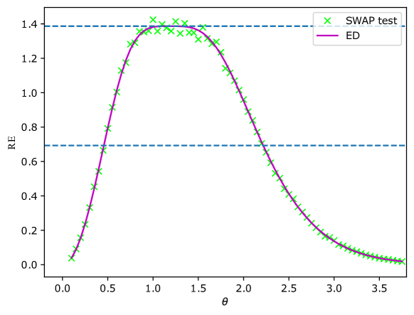
Figure 10: RE - SWAP test, 20000 shots per iteration. The quench is performed from the $|0000\rangle$ state for the L=4 OBC circuit, $\alpha$=1.2, $\gamma$=20. Blue dashed lines represent multiples of $\log(2)$

Figure 11: An instance of the SWAP circuit on two copies of a 4-qubit OBC system

6 Outlook

In this paper we embarked on the analysis of a class of unitary brick wall quantum circuits that are built using the scattering data ($S$-matrices) of integrable supersymmetric particle theories in 1+1D. The resulting unitaries $\mathbf{U_{F}}(\alpha,\gamma,\theta)$ have an underlying free fermionic (or fermionic gaussian or matchgate) structure. The supersymmetry of the 1+1D particle theory translates into a global fermionic symmetry, which protects the criticality of two hamiltonian operators associated to $\mathbf{U_{F}}$: the ‘Floquet’ hamiltonian $\mathbf{E}(\alpha,\gamma,\theta)$ and the logarithmic derivative $\mathbf{H_{\gamma}}(\alpha,\gamma)$ (see eq. 3.1). The latter simplifies to the Kitaev chain hamiltonian $\mathbf{H_{0}}(\alpha)$ for $\gamma=0$. We also displayed topological phases (in the BDI class) that arise upon breaking the global fermionic symmetry (but keeping the free fermionic form).

The (ground state) phase diagrams of (perturbations of) $\mathbf{E}(\alpha,\gamma,\theta)$ and $\mathbf{H_{\gamma}}(\alpha,\gamma)$ deserve further study. Perturbations may include terms beyond the free fermionic realm, similar to those considered for the Kitaev chain in [13, 29].

Section 4 of this paper explored a few simple examples of the quantum dynamics set by $\mathbf{U_{F}}(\alpha,\gamma,\theta)$, focusing on the build-up of entanglement entropy from the all-zero state for small systems. Clearly, the free fermionic structure will set a generalized Gibbs ensemble (GGE) constraining the dynamics. It will be interesting to scout the effects on the quantum dynamics of special features in the spectral structure of the brick wall unitaries that we unveiled in our analysis in this paper. Extending our set-up to monitored circuits (keeping the underlying free fermion structure and the analytic control that it brings) is another promising direction.

Appendix A Graded Floquet Baxterization with periodic boundary conditions

In this appendix we generalize the Floquet Baxterization thereom of [15] to the case of a graded space. We adhere to the notation of [15], naming the solution to the Yang-Baxter equation $\mathbf{\check{R}}$ rather than $\mathbf{\check{S}}$.

Theorem A.1 (Graded Floquet Baxterization).

For a unitary and invertible $\mathbf{\check{R}}$-matrix in a $\mathbb{Z}_{2}$ graded space such that $p(\mathbf{\check{R}}(u))=0$, the periodic time evolution operator of a system of size $L$, with $L\mod 2=0$ and $\mathbf{\check{R}}(u)=\mathbf{\Pi}\mathbf{R}(u)$:

$$\mathbf{\hat{U}_{F}}(\theta_{1}-\theta_{2})=\left(\prod_{i=1}^{L/2}\mathbf{\check{R}}_{2i-1,2i}(\theta_{1}-\theta_{2})\right)\left(\prod_{i=1}^{L/2}\mathbf{\check{R}}_{2i,2i-1}(\theta_{1}-\theta_{2})\right)\,,$$ (A.1)

is integrable, i.e.

$$\left[\mathbf{\hat{U}_{F}}(\theta_{1},\theta_{2}),\mathbf{t}(u,\theta_{1},\theta_{2})\right]=0\,, \Big{[}\mathbf{t}(u,\theta_{1},\theta_{2}),\mathbf{t}(v,\theta_{1},\theta_{2})\Big{]}=0\,,$$ (A.2)

with the transfer matrix evaluated with:

$$\mathbf{t}(u,\theta_{1},\theta_{2})=\mathrm{Tr}^{\mathrm{s}}\left[\mathbf{T_{a}}(u,\theta_{1},\theta_{2})\right]\,, \mathbf{T_{a}}(u,\theta_{1},\theta_{2})=\prod_{i=L}^{1}\mathbf{R}_{a,i}(u,\theta_{j})\,,\;\;\;j=i\mod 2\,.$$ (A.3)

We remark that the monodromy matrix in equation A.3 is made up by R-matrices and since each one of them acts both on the auxiliary space $\mathcal{H}_{a}$ and one physical qubit $\mathcal{H}_{i}$ their form is not trivial. In fact even if $p(\mathbf{R}(u))=0$ when only one of the two subspaces is permuted if $\mathbf{R}(u)$ has non diagonal terms there will be extra minus signs, from equation 2.4. Explicitly the product will be written as [4]:

$$\left(\mathbf{T_{a}}(u,\theta_{1},\theta_{2})\right)_{\alpha\mathbf{a}}^{\beta\mathbf{b}}=\left(\mathrm{Tr^{s}}_{a}\left[\prod_{i=L}^{1}\mathbf{R}_{a,i}(u-\theta_{j})\right]\right)_{\alpha\mathbf{a}}^{\beta\mathbf{b}}{(-1)}^{\sum_{j=2}^{L}(p(a_{j})+p(b_{j}))\sum_{i=1}^{j-1}p(a_{j})}\,.$$ (A.4)

Proof.

We start by defining the operator $\mathbf{W}(\theta_{1},\theta_{2})$ acting on the graded Hilbert space $\left(\mathbb{C}^{(1|1)}\right)^{\otimes L}$:

$$\mathbf{W}(\theta_{1},\theta_{2})=\mathbf{\tilde{G}}\prod_{i=1}^{L/2}\mathbf{\check{R}}_{2m-1,2m}(\theta_{1},\theta_{2})\,, \mathbf{\tilde{G}}=\prod_{m}^{L-1}\mathbf{\Pi}_{m,m+1}$$ (A.5)

where $\mathbf{\tilde{G}}$ is the graded translation operator. We now want to introduce an operator $\mathbf{\tilde{W}}$ that acts on a bigger Hilbert space $\mathcal{H}_{b}\otimes\left(\mathbb{C}^{(1|1)}\right)^{\otimes L}$, to define $\mathbf{W}$ as we define the transfer matrix with the monodromy matrix:

$$\mathbf{\tilde{W}}_{b}(u_{1},u_{2})=\prod_{i=L/2}^{1}\mathbf{R}_{b,2m}(\theta_{1},\theta_{2})\mathbf{\Pi}_{b,2m-1}\,.$$ (A.6)

Knowing that $\mathbf{R}_{i,j}=\mathbf{\Pi}_{i,j}\mathbf{\check{R}}_{i,j}$ we get for each term of the product:

$$\mathbf{R}_{b,2m}\mathbf{\Pi}_{b,2m-1} =\mathbf{\Pi}_{b,2m}\mathbf{\check{R}}_{b,2m}\mathbf{\Pi}_{b,2m-1}\,,$$

$$=\mathbf{\Pi}_{b,2m}\mathbf{\Pi}_{b,2m-1}\mathbf{\Pi}_{b,2m-1}\mathbf{\check{R}}_{b,2m-1}\mathbf{\Pi}_{b,2m-1}\,,$$

$$=\mathbf{\Pi}_{b,2m}\mathbf{\Pi}_{b,2m-1}\mathbf{\check{R}}_{2m-1,2m}\,.$$ (A.7)

So plugging in this result in the equation for each pair of R and $\mathbf{\Pi}$, we get:

$$\mathbf{\tilde{W}}_{b}(\theta_{1},\theta_{2})=\prod_{i=L}^{1}\mathbf{\Pi}_{b,i}\prod_{i=1}^{L/2}\mathbf{\check{R}}_{2m-1,2m}(\theta_{1},\theta_{2})\,.$$ (A.8)

Now using the train trick A.7 we can rewrite the previous expression as:

$$\mathbf{\tilde{W}}_{b}(\theta_{1},\theta_{2})=\mathbf{\Pi}_{b,1}\mathbf{\tilde{G}}\prod_{i=1}^{L/2}\mathbf{\check{R}}_{2m-1,2m}(\theta_{1},\theta_{2})\,.$$ (A.9)

We underline that the order of the product of the bricks doesn’t matter, since they act on different subspaces, thus we get the relation:

$$\mathbf{W}(\theta_{1},\theta_{2})=\mathrm{Tr^{s}}_{b}\left[\mathbf{\tilde{W}}_{b}(\theta_{1},\theta_{2})\right]\,.$$ (A.10)

Now the key relation that makes the system integrable is an equation similar to Yang-Baxter. In fact one can show that for a graded R-matrix,

$$\mathbf{R}_{a,b}(u,\theta_{1})\mathbf{R}_{a,m}(u,\theta_{1})\mathbf{\Pi}_{b,m}=\mathbf{\Pi}_{b,m}\mathbf{R}_{a,m}(u,\theta_{1})\mathbf{R}_{a,b}(u,\theta_{1})\,.$$ (A.11)

Therefore one can reproduce the intertwining relation between inhomogeneous monodromy matrices [20] with the newly introduced operator $\mathbf{\tilde{W}}_{b}(\theta_{1},\theta_{2})$,

$$\mathbf{R}_{a,b}(u,\theta_{1})\mathbf{M}_{a,m}(u,\theta_{1},\theta_{2})\mathbf{\tilde{W}}_{b}(\theta_{1},\theta_{2})=\mathbf{\tilde{W}}_{b}(\theta_{1},\theta_{2})\mathbf{M}_{a,m}(u,\theta_{1},\theta_{2})\mathbf{R}_{a,b}(u,\theta_{1}).$$ (A.12)

Now multiplying this last equation from the left and taking the super partial trace on both sides one get:

$$\left[\mathbf{T}\left(u,\theta_{1},\theta_{2}\right),\mathbf{W}\left(\theta_{1},\theta_{2}\right)\right]=0\,.$$ (A.13)

From construction the transfer matrix commutes with the graded translation operator squared,

$$\left[\mathbf{T}\left(u,\theta_{1},\theta_{2}\right),\mathbf{\tilde{G}}^{2}\right]=0\,,$$ (A.14)

and naturally also with its inverse $\mathbf{\tilde{G}}^{-2}$. The square of the operator now we notice that the operator $\mathbf{W}(\theta_{1},\theta_{2})$ is essentially the even layer of the brick wall multiplied by the graded translation operator. Taking the square of it and multiplying it from the left by $\mathbf{\tilde{G}}^{-2}$ will give us:

$$\begin{split}\mathbf{\tilde{G}}^{-2}\mathbf{W}^{2}\left(\theta_{1},\theta_{2}\right)&=\mathbf{\tilde{G}}^{-1}\left(\prod_{i=1}^{L/2}\mathbf{\check{R}}_{2m-1,2m}(\theta_{1},\theta_{2})\right)\mathbf{\tilde{G}}\left(\prod_{i=1}^{L/2}\mathbf{\check{R}}_{2m-1,2m}(\theta_{1},\theta_{2})\right),\\ &=\left(\prod_{i=1}^{L/2}\mathbf{\check{R}}_{2m,2m+1}(\theta_{1},\theta_{2})\right)\left(\prod_{i=1}^{L/2}\mathbf{\check{R}}_{2m-1,2m}(\theta_{1},\theta_{2})\right),\\ &=\mathbf{U_{F}}(\theta_{1},\theta_{2}).\end{split}$$ (A.15)

Therefore,

$$\left[\mathbf{T}\left(u,\theta_{1},\theta_{2}\right),\mathbf{U_{F}}(\theta_{1},\theta_{2})\right]=0\,,$$ (A.16)

$\forall u\in\mathbb{C}$. ∎

We remark that in the theorem we imposed the condition $p(\mathbf{R}(u))=0$ because when this condition does not hold we have to deal with the minus signs from equation 2.4. That would mean that the representation in ungraded space of the R-matrix would not be local anymore. This would make the implementation of the quantum brick wall circuit unfeasible.

Appendix B Explicit form of $\mathbf{H_{\gamma}}$

B.1 Real space form and coefficients

The hamiltonian in equation 3.9 can be expressed as a linear combination of local Pauli matrices. Writing it in block diagonal form and then applying a Jordan-Wigner transformation (2.21) the real space hamiltonian results:

$$\begin{split}\mathbf{H_{\gamma}}=\sum_{i}&\bigg{[}-N_{A}c_{2i-1}^{\dagger}c_{2i-1}-N_{B}c_{2i}^{\dagger}c_{2i}+J_{AB}\left(c_{2i-1}^{\dagger}c_{2i}+c_{2i}^{\dagger}c_{2i-1}\right)\\ &+J_{BA}\left(c_{2i}^{\dagger}c_{2i+1}+c_{2i+1}^{\dagger}c_{2i}\right)+J_{AB}^{L}\left(c_{2i-1}^{\dagger}c_{2i+2}+c_{2i+2}^{\dagger}c_{2i-1}\right)\\ &+J_{AA}\left(c_{2i-1}^{\dagger}c_{2i+1}+c_{2i+1}^{\dagger}c_{2i-1}-c_{2i}^{\dagger}c_{2i+2}-c_{2i+2}^{\dagger}c_{2i}\right)\\ &+iS_{AB}\left(c_{2i-1}^{\dagger}c_{2i}^{\dagger}-c_{2i}c_{2i-1}\right)+iS_{BA}\left(c_{2i}^{\dagger}c_{2i+1}^{\dagger}-c_{2i+1}c_{2i}\right)\\ &+iS_{AA}\left(c_{2i-1}^{\dagger}c_{2i+1}^{\dagger}-c_{2i+1}c_{2i-1}-c_{2i}^{\dagger}c_{2i+2}^{\dagger}+c_{2i+2}c_{2i}\right)\\ &+S_{AB}^{L}\left(c_{2i-1}^{\dagger}c_{2i+2}^{\dagger}+c_{2i+2}c_{2i-1}\right)\bigg{]}+\frac{L}{4}(N_{A}+N_{B})\,.\end{split}$$ (B.1)

This hamiltonian is clearly free fermionic and its coefficient are functions of the parameters $\alpha$ and $\gamma$, explicitly:

$$N_{A} =\frac{\operatorname{sech}\left(\frac{\gamma}{2}\right)-\tanh\left(\frac{\gamma}{2}\right)\operatorname{sech}^{3}\left(\frac{\gamma}{2}\right)}{\alpha} N_{B} =\frac{\operatorname{sech}\left(\frac{\gamma}{2}\right)+\tanh\left(\frac{\gamma}{2}\right)\operatorname{sech}^{3}\left(\frac{\gamma}{2}\right)}{\alpha}$$

$$J_{AB} =\frac{3\tanh^{2}\left(\frac{\gamma}{2}\right)\operatorname{sech}^{2}\left(\frac{\gamma}{2}\right)+\operatorname{sech}^{4}\left(\frac{\gamma}{2}\right)}{2\alpha} J_{BA} =\frac{\operatorname{sech}^{4}\left(\frac{\gamma}{2}\right)}{2\alpha}$$

$$J_{AA} =\frac{\tanh\left(\frac{\gamma}{2}\right)\operatorname{sech}^{3}(\frac{\gamma}{2})}{2\alpha} J_{AB}^{L} =-\frac{\tanh^{2}(\frac{\gamma}{2})\operatorname{sech}^{2}\left(\frac{\gamma}{2}\right)}{2\alpha}$$

$$S_{AB} =\frac{\operatorname{sech}\left(\frac{\gamma}{2}\right)}{2} S_{BA} =\frac{\operatorname{sech}^{3}(\frac{\gamma}{2})}{2}$$

$$S_{AA} =\frac{\tanh\left(\frac{\gamma}{2}\right)\operatorname{sech}^{2}(\frac{\gamma}{2})}{2} S_{AB}^{L} =-\frac{\tanh^{2}\left(\frac{\gamma}{2}\right)\operatorname{sech}(\frac{\gamma}{2})}{2}.$$ (B.2)

B.2 Momentum space and dispersion relation coefficients

The hamiltonian 3.18 is the Fourier transform of equation B.1 written after a double folding of the Brillouin zone, its coefficients are:

$$N_{1} =\frac{\text{sech}^{4}\left(\frac{\gamma}{2}\right)\left(-4\cosh^{3}\left(\frac{\gamma}{2}\right)+(3\cosh(\gamma)+1)\cos(k)-2\sinh^{2}\left(\frac{\gamma}{2}\right)\cos(3k)\right)}{4\alpha}$$

$$N_{2} =\frac{\text{sech}^{4}\left(\frac{\gamma}{2}\right)\left(-4\cosh^{3}\left(\frac{\gamma}{2}\right)-(3\cosh(\gamma)+1)\cos(k)+2\sinh^{2}\left(\frac{\gamma}{2}\right)\cos(3k)\right)}{4\alpha}$$

$$H =-\frac{\tanh\left(\frac{\gamma}{2}\right)\text{sech}^{3}\left(\frac{\gamma}{2}\right)\left(\sinh^{2}(\frac{\gamma}{2})+2i\sinh\left(\frac{\gamma}{2}\right)\sin^{3}(k)+\cos(2k)\right)}{\alpha}$$

$$S_{1} =-\operatorname{sech}^{3}\left(\frac{\gamma}{2}\right)\sin(k)(1-\sinh^{2}(\frac{\gamma}{2})\cos(2k))$$

$$S_{2} =2\sinh\left(\frac{\gamma}{2}\right)\operatorname{sech}^{3}\left(\frac{\gamma}{2}\right)\sin(k)\cos(k)\left(1+i\sinh\left(\frac{\gamma}{2}\right)\sin(k)\right).$$ (B.3)

The diagonalization of the two $4\times 4$ blocks in terms of the coefficients appearing above results in:

$$\begin{split}\epsilon&=\pm\Bigg{(}\frac{N_{1}^{2}}{2}+\frac{N_{2}^{2}}{2}+|H|^{2}+S_{1}^{2}+|S_{2}|^{2}\pm\frac{1}{2}\Big{(}(N_{1}^{2}-N_{2}^{2})^{2}+4(N_{1}+N_{2})^{2}|H|^{2}\\ &\quad\quad+16S_{1}^{2}|H|^{2}-16(N_{1}-N_{2})S_{1}\mathrm{Re}\left[S_{2}H^{*}\right]-8\mathrm{Re}\left[S_{2}^{2}(H^{*})^{2}\right]\\ &\quad\quad+4(N_{1}-N_{2})^{2}|S_{2}|^{2}+8|H|^{2}|S_{2}|^{2}\Big{)}^{\frac{1}{2}}\Bigg{)}^{\frac{1}{2}}\,.\end{split}$$ (B.4)

Now plugging inside the equation above the values of the coefficients we find the expression in equation 3.11, with the following coefficients

$$\nu_{0} =\frac{\text{sech}^{4}\left(\frac{\gamma}{2}\right)}{\alpha^{2}}\left(1+2\cosh(\gamma)\right)+\text{sech}^{2}\left(\frac{\gamma}{2}\right),$$

$$\nu_{1} =\frac{\text{sech}^{4}\left(\frac{\gamma}{2}\right)}{\alpha^{2}}-\text{sech}^{2}\left(\frac{\gamma}{2}\right),$$

$$\begin{split}\mu_{0}&=\frac{\operatorname{sech}^{6}\left(\frac{\gamma}{2}\right)}{\alpha^{4}}\left(8\cosh(\gamma)\right)\\ &\quad+\frac{\tanh^{2}\left(\frac{\gamma}{2}\right)\operatorname{sech}^{12}\left(\frac{\gamma}{2}\right)}{32\alpha^{2}}\Big{(}300-193\cosh(\gamma)+162\cosh(2\gamma)-15\cosh(3\gamma)+2\cosh(4\gamma)\Big{)},\end{split}$$

$$\begin{split}\mu_{1}&=\frac{8\operatorname{sech}^{6}\left(\frac{\gamma}{2}\right)}{\alpha^{4}}\\ &\quad-\frac{\tanh^{2}\left(\frac{\gamma}{2}\right)\text{sech}^{12}\left(\frac{\gamma}{2}\right)}{16\alpha^{2}}\Big{(}163-120\cosh(\gamma)+92\cosh(2\gamma)-8\cosh(3\gamma)+\cosh(4\gamma)\Big{)},\end{split}$$

$$\mu_{2} =\frac{\tanh^{4}\left(\frac{\gamma}{2}\right)\text{sech}^{10}\left(\frac{\gamma}{2}\right)}{16\alpha^{2}}\Big{(}93+4\cosh(\gamma)+31\cosh(2\gamma)\Big{)},$$

$$\mu_{3} =-\frac{\tanh^{4}\left(\frac{\gamma}{2}\right)\text{sech}^{10}\left(\frac{\gamma}{2}\right)}{2\alpha^{2}}\Big{(}21-12\cosh(\gamma)+7\cosh(2\gamma)\Big{)},$$

$$\mu_{4} =\frac{\tanh^{4}\left(\frac{\gamma}{2}\right)\text{sech}^{10}\left(\frac{\gamma}{2}\right)}{8\alpha^{2}}\Big{(}45-44\cosh(\gamma)+15\cosh(2\gamma)\Big{)},$$

$$\mu_{5} =-\frac{4\tanh^{8}\left(\frac{\gamma}{2}\right)\text{sech}^{6}\left(\frac{\gamma}{2}\right)}{\alpha^{2}},$$

$$\mu_{6} =\frac{\tanh^{8}\left(\frac{\gamma}{2}\right)\text{sech}^{6}\left(\frac{\gamma}{2}\right)}{2\alpha^{2}}.$$ (B.5)

References

- [1] S. Aaronson and A. Arkhipov “The Computational Complexity of Linear Optics” In Proceedings of the Forty-Third Annual ACM Symposium on Theory of Computing Association for Computing Machinery, 2011 DOI: 10.1145/1993636.1993682
- [2] S. Aaronson and D. Gottesman “Improved simulation of stabilizer circuits” In Phys. Rev. A 70 American Physical Society, 2004 DOI: 10.1103/PhysRevA.70.052328
- [3] J.L. Cardy and G. Mussardo “S-matrix of the Yang-Lee edge singularity in two dimensions” In Physics Letters B 225.3, 1989 DOI: https://doi.org/10.1016/0370-2693(89)90818-6
- [4] F… Essler and V.. Korepin “A New Solution of the Supersymmetric TJ Model by Means of the Quantum Inverse Scattering Method” arXiv, 1992
- [5] B.U. Felderhof “Diagonalization of the transfer matrix of the free-fermion model. II” In Physica 66.2, 1973, pp. 279–297 DOI: https://doi.org/10.1016/0031-8914(73)90330-3
- [6] B.U. Felderhof “Diagonalization of the transfer matrix of the free-fermion model. III” In Physica 66.3, 1973 DOI: https://doi.org/10.1016/0031-8914(73)90298-X
- [7] B.U. Felderhof “Direct diagonalization of the transfer matrix of the zero-field free-fermion model” In Physica 65.3, 1973 DOI: https://doi.org/10.1016/0031-8914(73)90059-1
- [8] D. Gottesman “The Heisenberg representation of quantum computers”, 1998 URL: https://www.osti.gov/biblio/319738
- [9] V. Gritsev and A. Polkolnikov “Integrable Floquet Dynamics” In SciPost Phys. 2, 2017 DOI: 10.21468/SciPostPhys.2.3.021
- [10] R. Jozsa and A. Miyake “Matchgates and classical simulation of quantum circuits” In Proceedings of the Royal Society A: Mathematical, Physical and Engineering Sciences 464.2100, 2008, pp. 3089–3106 DOI: 10.1098/rspa.2008.0189
- [11] A.. Kitaev “Unpaired Majorana fermions in quantum wires” In Physics-Uspekhi 44.10S, 2001 DOI: 10.1070/1063-7869/44/10S/S29
- [12] X.S. Li et al. “Topological properties of the dimerized Kitaev chain with long-range couplings” In Results in Physics 30, 2021 DOI: https://doi.org/10.1016/j.rinp.2021.104837
- [13] I. Mahyaeh and E. Ardonne “Zero modes of the Kitaev chain with phase-gradients and longer range couplings” In Journal of Physics Communications 2.4 IOP Publishing, 2018 DOI: 10.1088/2399-6528/aab7e5
- [14] K. Maruyoshi et al. “Conserved charges in the quantum simulation of integrable spin chains” In Journal of Physics A: Mathematical and Theoretical 56, 2023 DOI: 10.1088/1751-8121/acc369
- [15] Y. Miao, V. Gritsev and D.. Kurlov “The Floquet Baxterisation” arXiv, 2022 DOI: 10.48550/arXiv.2206.15142
- [16] M. Moriconi and K. Schoutens “Reflection matrices for integrable N = 1 supersymmetric theories” In Nuclear Physics B 487.3, 1997, pp. 756–778 DOI: https://doi.org/10.1016/S0550-3213(96)00632-3
- [17] M. Moriconi and K. Schoutens “Thermodynamic Bethe Ansatz for N = 1 supersymmetric theories” In Nuclear Physics B 464.3, 1996 DOI: https://doi.org/10.1016/0550-3213(95)00649-4
- [18] B. Pozsgay “Quantum circuits with free fermions in disguise”, 2024 DOI: https://doi.org/10.48550/arXiv.2402.02984
- [19] K. Schoutens “Supersymmetry and factorizable scattering” In Nuclear Physics B 344.3, 1990 DOI: 10.1016/0550-3213
- [20] N. Slavnov “Algebraic Bethe Ansatz and Correlation Functions” World Scientific, 2022
- [21] B.. Terhal and D.. DiVincenzo “Classical simulation of noninteracting-fermion quantum circuits” In Phys. Rev. A 65 American Physical Society, 2002 DOI: 10.1103/PhysRevA.65.032325
- [22] S. Tewari and J.. Sau “Topological Invariants for Spin-Orbit Coupled Superconductor Nanowires” In Phys. Rev. Lett. 109 American Physical Society, 2012 DOI: 10.1103/PhysRevLett.109.150408
- [23] L.. Valiant “Quantum Circuits That Can Be Simulated Classically in Polynomial Time” In SIAM Journal on Computing 31.4, 2002 DOI: 10.1137/S0097539700377025
- [24] M. Van den Nest “Universal Quantum Computation with Little Entanglement” In Phys. Rev. Lett. 110 American Physical Society, 2013 DOI: 10.1103/PhysRevLett.110.060504
- [25] M. Vanicat, L. Zadnik and T. Prosen “Integrable Trotterization: Local Conservation Laws and Boundary Driving” In Phys. Rev. Lett. 121, 2018 DOI: 10.1103/PhysRevLett.121.030606
- [26] E. Vernier, B. Bertini, G. Giudici and L. Piroli “Integrable Digital Quantum Simulation: Generalized Gibbs Ensembles and Trotter Transitions” In Phys. Rev. Lett. 130 American Physical Society, 2023 DOI: 10.1103/PhysRevLett.130.260401
- [27] G. Vidal “Efficient Classical Simulation of Slightly Entangled Quantum Computations” In Phys. Rev. Lett. 91 American Physical Society, 2003 DOI: 10.1103/PhysRevLett.91.147902
- [28] R. Wakatsuki, M. Ezawa, Y. Tanaka and N. Nagaosa “Fermion fractionalization to Majorana fermions in a dimerized Kitaev superconductor” In Phys. Rev. B 90 American Physical Society, 2014 DOI: 10.1103/PhysRevB.90.014505
- [29] J. Wouters, H. Katsura and D. Schuricht “Exact ground states for interacting Kitaev chains” In Physical Review B 98.15 American Physical Society (APS), 2018 DOI: 10.1103/physrevb.98.155119
- [30] A.. Zamolodchikov “Integrals of motion and S-matrix of the (scaled) T=Tc Ising model with magnetic field” In International Journal of Modern Physics A 4.16, 1989