AN ONE-STEP IMAGE RETARGETING ALGORITHM BASED ON CONFORMAL ENERGY
Abstract
The image retargeting problem is to find a proper mapping to resize an image to one with a prescribed aspect ratio, which is quite popular these days. In this paper, we propose an efficient and orientation-preserving one-step image retargeting algorithm based on minimizing the harmonic energy, which can well preserve the regions of interest (ROIs) and line structures in the image. We also give some mathematical proofs in the paper to ensure the well-posedness and accuracy of our algorithm.
Keywords: Image retargeting, conformal energy, simplicial approximation, one-step algorithm
1 Introduction
Nowadays, there are more and more electronic devices with different screen ratios. It may cause visual unnaturality and geometric information loss of the result images, like the images in a distorting mirror, to display one picture on different devices by simply stretching it into the ratio we want thus giving rise to the need for more image retargeting algorithms, which can resize images into different sizes while preserving some properties of original images.
Various methods have been developed to tackle this problem, which can mainly be divided into two categories: cropping-based methods and mesh-based warping methods.
Cropping-based methods are to remove unimportant pixels and reset the other pixels to resize the image. Taking the popular Seam Carving algorithm [1] proposed by Avidan and Shamir as an example, it searches for the least important seams and removes them, but sometimes the important objects in the image may be destroyed when seams accidentally pass through important areas. The retargeting maps in these methods are not bijective, which means some informaiton contained in images will be lost.
The mesh-based warping methods aim to divide images by triangular or quadrilateral mesh and compute the vertex coordinates to resize images. The geometric distortion in important areas is minimized, while larger distortion is allowed in unimportant areas. conformal and quasi-conformal mapping can well control the local geometric distortion, so it is proper for the retargeting problem. Xu proposed a new image retargeting method based on quasi-conformal mapping obtained by solving an optimization problem in [17]. Lau[8] developed one more efficient one-step quasi-conformal mapping retargeting method. However, the difference between conformal mapping and harmonic mapping is ignored in these two papers, which will result in huge errors about quasi-conformal warping maps. Additionally, the linear Beltrami solver has been applied in both of these two methods, while the maps generated by the linear Beltrami solver are not theoretically ensured to be orientation-preserving. Here, we can give a counterexample 1 generated by the linear Beltrami solver from a Beltrami coefficient whose norm is less than 1.
2 Background
2.1 Mathematical modeling
We build up one mathematical model to illustrate the image retargeting problems.
ROIs, usually the main objects in one image, are the critical parts that attract most people’s attention at first sight. Therefore, it is reasonable to preserve the shapes of those objects entirely during the retargeting process. Line structures are another important factor in images. The human visual system is sensitive to distortions except stretching, so we set the warping map on the line structure as a simple stretching mapping.
We can only adjust the width of images to get images with the target aspect ratio. Denote that the region of original image is , and the region of output of retargeting algorithm is , where is the resizing ratio. Suppose an image is defined on . The target image is defined on . The ROIs in are and line structures are . Let , and . are disjoint sets.
The retargeting map is a bijective warping map . The ROIs and line constraints can be illustrated in two formulas below,
| (1) | ||||
in which , is a 22 diagonal matrix, whose diagonal elements are all positive, and , , . These parameters are given in advance. For the boundary constraint, the boundary condition should be a bijective continuous map, which satisfies .
Since the geometric distortion in is inevitable, we want to make the distortion distribution over as even as possible. Therefore, we introduce conformal energy to our model to achieve this goal.
2.2 Conformal Energy
Given a map such that and , conformal energy functional is the measure of local geometric distortion of function . According to [6], conformal energy is defined by
| (2) | ||||
where as the Dirichlet energy of and . Especially, if and only if is a conformal mapping.
3 One-step Retargeting Algorithm
In this section, we will introduce the body of the one-step retargeting algorithm. Firstly, we will use simplicial mapping to approximate the conformal energy minimizer in the continuous set. Then, we need to do the bijection correction to the simplicial approximation. In the case that the parameters are not given, we can initialize these parameters by solving equations 17.
3.1 Minimizer in the continuous set
In the retargeting problem, the feasible region of is set to be . The parameters are all determined in advance. The optimization problem can be illustrated by the following formulas:
| (3) | ||||
| s. t. | ||||
3.2 Discretization
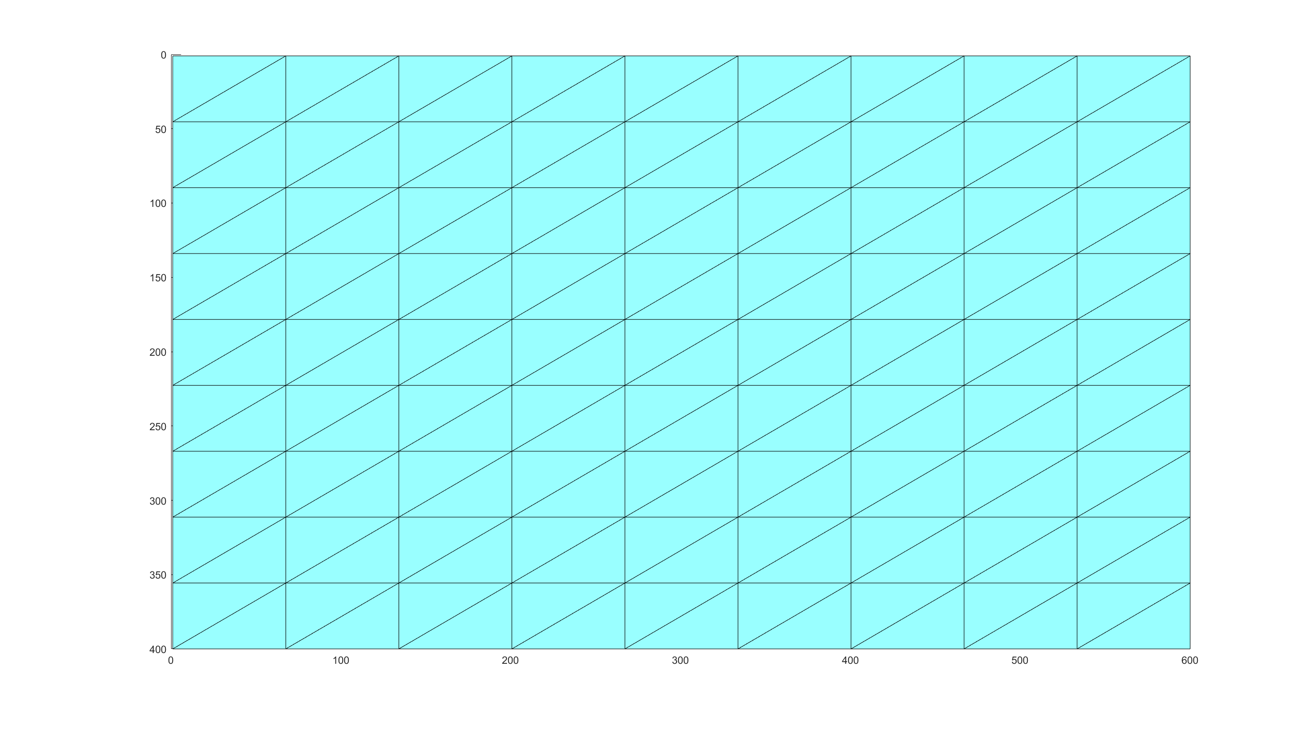
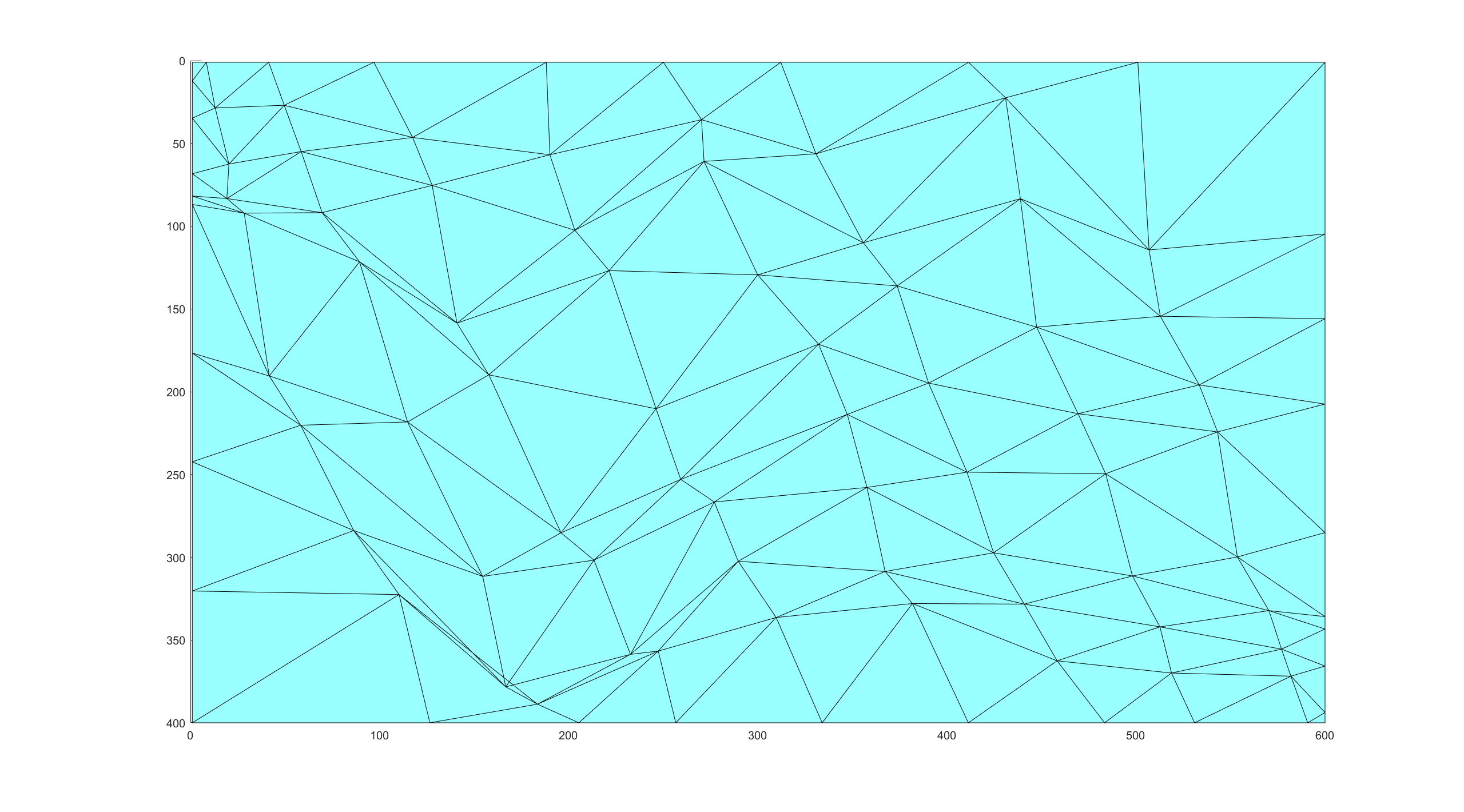
In the image retargeting problem, and are two rectangles with different aspect ratios. We discretize with simply connected Delaunay triangulation mesh to make it computable[4].
| (4) |
is the vertexes part, is defined to be the edges part, and
| (5) |
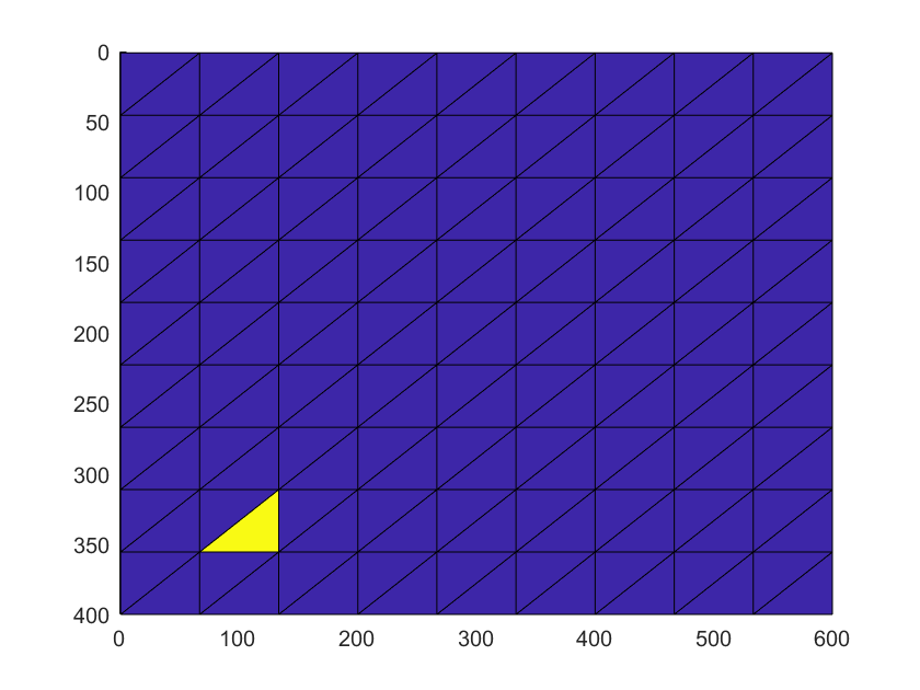
denotes the simplices in the mesh, where
| (6) |
The triangular faces cover the domain of mapping , which means and , where
For ROIs part, we define , and . As for line structures, , and . The boundary part is . is the rest part of the mesh. Suppose
are disjoint sets. Therefore, we have the ROI, line structure, and boundary constraints on mesh:
| (7) | ||||
Let a simplicial mapping be the affine interpolant of on mesh :
| (8) | |||
In other words, for the simplex , , where and , in which are translation coefficients of and
| (9) |
is the first derivative of , where
| (10) | ||||
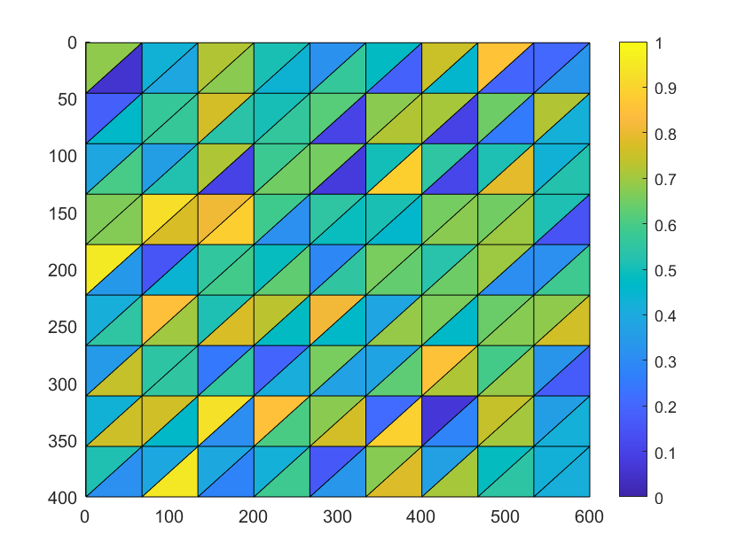
Discrete conformal energy on mesh is defined as
| (11) |
3.3 Minimizer in the discrete set
In the discrete set, we want to get the optimal simplicial mapping on mesh . Denote the discrete feasible region as . The simplicial mapping can be written in matrix form , in which , ; and .
In fact, discrete conformal energy is a quadratic polynomial with respect to , which means we can solve a system of linear equations to find the optimized simplicial mapping. This ensures that the computational complexity of the algorithm is acceptable for real-time computing.
The linear equations are listed below:
| (12) | ||||
where .
Then, the equations can be presented as follows:
| (13) |
where is a matrix, whose entries satisfy
| (14) |
and is a zero matrix.
Denote that , where and . Correspondingly, the matrix can be written in the form of a block matrix: , where is the first columns of , so we have
| (15) |
If we can prove is inevitable, we can ensure the uniqueness and existence of the minimizer in the discrete set, which will be talked about later.
3.4 Bijection correction algorithm
In a few experiments, the optimal simplicial mapping may not be a bijective function due to low mesh accuracy or extreme constraints. To ensure the warping map is bijective and orientation-preserving, we introduce the bijection correction of simplicial mapping, which will relax the ROI and line constraints to ensure the bijection at the expense of the shape of ROIs and line structures.
We initialize the constraints relaxation set as and the iterative step is . If the output of the conformal energy minimizer is not orientation-preserving, we will start our iterative bijection correction algorithm. The corrected function is generated by equations:
| (16) |
Then, we will check whether is orientation-preserving. If so, we will set it as the final output; otherwise, we will go to another step of the iterative method.
3.5 ROIs, line structures and boundary condition
ROIs and line structures can be either manually marked or automatically detected. For ROI detection, the saliency map is a powerful tool ([7], [5]). It can be calculated by the algorithm given in [11]. We can set a threshold and select the parts whose value of the saliency map exceeds the threshold as ROIs. Line structures can be realized by Hough transform or other algorithms.
The parameters in the model and boundary condition can be fixed in advance or calculated by some algorithm. Here, we give an initialization method to determine these parameters.
We can use the least squares method to find the constrained map, which is the closest one to the discrete harmonic map. In other words, we can initialize these parameters by computing the approximate solution to the overdetermined system:
| (17) |
where is the normal vector of at , and
then, we can set the boundary condition as .
4 Analysis of Model
4.1 Existence and uniqueness of the minimizer in the continuous set
Since , , and are fixed, the constrained optimization problem (3) can be translated into another form:
| (18) | ||||
| s. t. | ||||
where equals plus a constant.
Proposition 4.1.
and conformal energy are non-negative and strongly convex functionals.
Theorem 4.1.
(Banach-Alaoglu Theorem) Let be a Banach space. Then the unit ball of is compact in the topology.
Theorem 4.2.
(Rellich-Kondrachov theorem) Let be a bounded Lipschitz domain, the embedding is compact and continuous.
Assumption 4.1.
is a bounded set with Lipschitz boundary
Theorem 4.3.
(Existence and uniqueness of the minimizer in the continuous set) If Assumption 4.1 holds, there exists one and only one minimizer of conformal energy .
Proof.
In the bounded set with Lipschitz boundary, because , for any there exists a sequence of functions such that and , so there exists such that because of Poincaré inequality. By Theorem 4.1, we can have which satisfies . By Theorem 4.2, in the sence of strongly convergence in . Due to the fact that , we can get with respect to norm. , so in the sence of strongly convergence in . is a close set in , so we can have . For any , , so is continuous in . Therefore, . Due to arbitrariness of , we have . Therefore, we can get . The existence of the minimizer holds.
By Proposition 4.1, is a strongly convex functional, so the uniqueness of the minimizer is also ensured.
Because equals plus a constant, the unique minimizer of is also the minimizer of . ∎
Therefore, we can claim the existence and uniqueness of the minimizer in the continuous set. Denote the minimizer as in .
4.2 Existence and uniqueness of the minimizer in the discrete set
Then, we prove the existence and uniqueness of the conformal energy minimizer in the discrete set.
Lemma 4.1.
is a principal submatrix of the Laplacian matrix
| (19) |
of the mesh mentioned in [18], where and are the two angles opposite to the edge connecting vertices and on the mesh ; .
Proof.
Suppose there are two adjacent simplices , then the corresponding entry of edge in is
| (20) | ||||
because is a Delaunay rectangular mesh and we have . ∎
Definition 4.1.
([2])
(i) A matrix is said to be nonnegative(positive) if all entries of are nonnegative(positive).
(ii) A matrix is said to be an M-matrix if , where is nonnegative and .
(iii) A matrix is said to be a Stieltjes matrix if it is a symmetric nonsingular M-matrix.
Lemma 4.2.
(Theorem 1.4.10 in [10]) Suppose is a singular, irreducible M-matrix. Then, each principal submatrix of other than itself is a nonsingular -matrix.
Theorem 4.4.
(Existence and uniqueness of the minimizer in the discrete set) is a Stieltjes matrix, and there is one and only one minimizer of , whose matrix form is:
| (21) |
The computational complexity of this minimizer is no greater than .
Proof.
From Lemma 4.3, we know that is a singular M-matrix. Because the mesh is connected, the adjacent matrix of graph is irreducible. Due to 4.1, the matrix can be represented as , where is a diagonal matrix and is a negative matrix whose diagonal entries are all 0. Since and has the following relationship:
| (22) |
is is irreducible too, so is a irreducible M-matrix. is a principal submatrix of , so is a nonsingular M-matrix by Lemma 4.2. We can find that is symmetric. In the end, we prove is a Stieltjes matrix and there is one and only one minimizer of , whose matrix form is:
| (23) |
For the computational complexity of the discrete minimizer, we can first get the inverse of by Cholesky decomposition, whose computational complexity is . Then, the complexity of matrix multiplication is also ; therefore, the total complexity is also . ∎
4.3 Point-wise convergence of to
Definition 4.2.
(Subdivision of simplicial complex[12]) simplicial complex is a subdivision of another simplicial complex , written , if and each cell of is contained in a cell of .
Definition 4.3.
(Corner-chopped subdivision of 3-simplicial complex) For the 3-simplicial complex mesh , its corner-chopped subdivision mesh
where are the barycenters of respectively.
Lemma 4.4.
(Convergence of maximum diameter of corner-chopped subdivision sequence) Denote that one mesh with bounded maximum diameter is and We have the maximum diameter satisfying
| (24) |
Proof.
For and , Since are the barycenters of respectively, we have and are parrallel and the length of is half of the length of . Therefore, triangular is similar to and the ratio of similitude is . The diameter of is half of . Similarly, we can get the diameter of every cell in is half of the diameter of its ”mother cell” in . Here, we can get that . Therefore, ∎
Lemma 4.5.
([15]) Let . If is weakly differentiable and if , then for any periodic triangulation mesh of , which is also a complex whose maximum diameter of all the simplices is less than , we have
| (25) |
where is the translated mesh of and . In particular,
| (26) |
This lemma illustrates that the simplicial mapping can approximate the mapping in very well, which gives the solid theoretical foundation of triangulation. For any triangulation of whose maximum diameter of simplices is very small, the piecewise affine interpolation of a mapping is likely to converge to itself. If not, we can translate the mesh until we find the convergent one. Therefore, it is reasonable to assume the periodic extension of the subdivision mesh of makes it convergent.
Assumption 4.2.
Denote is the periodic expansion of mesh , in which , in which , and is the trivial expansion of in : Suppose covering is a bounded maximum diameter mesh such that
| (27) |
Equivalently,
| (28) |
Theorem 4.5.
(Point-wise convergence of discrete conformal energy) Suppose the mesh satisfies the Assumption 4.2, denote , then we have
| (29) |
Proof.
If Assumption 4.2 holds,
| (30) |
and
| (31) | ||||
Additionally, because it is a is a non-negative integer, so . ∎
4.4 Convergence of and
In this section, we will talk about the convergence property of the minimizer of .
Let be the simplicial mapping space generated by the mesh which satisfies Assumption 4.2 and all of its subdivisions.
Assumption 4.3.
Suppose for any , and boundary condition satisfy the following conditions:
| (32) |
where and .
Lemma 4.6.
(Representation of with ) If Assumption 4.3 holds,
Proof.
As for any simplicial mapping , for ,
| (34) |
For ,
| (35) |
For ,
| (36) |
Therefore, we have . We also have , so . ∎
Lemma 4.7.
Proof.
From the proof of Lemma 4.6, we know that the ROIs, line structures, boundary conditions and constraints are all equivalent. We also have for , so . Therefore, .
Given the increasing sequence of sets , we have . By Assumption 4.2, holds, so . is a close set in , so . Finally, we get . ∎
Theorem 4.6.
Proof.
By Lemma 4.6, we have , so
From Lemma 4.7, we can know , so
Due to the existence and uniqueness in the continuous set (Theorem 4.3) and the discrete set (Theorem 4.4), and , so is a decreasing sequence with lower bound . By Assumption 4.2, there exists a sequence of functions such that . It is obvious that . Therefore, we can get by dominated convergence theorem.
Because , for any , there exists such that for any . is bounded open set with Lipschitz boundary, and the measure of is 0. There exists , such that the sequence of functions due to Poincaré inequality. Then, by Theorem 4.1, there exists a subsequence of such that . From Theorem 4.2, with respect to norm. We have . 2 In other words, with respect to norm. Since , we have in .
Because is a close set in , . By uniqueness of the minimizer of in , we have . Therefore, there exists a subsequence of such that . ∎
4.5 Analysis of bijection correction algorithm
We have three questions about the bijection correction algorithm: Can we ensure the output map is a bijection? Does the algorithm converge? If so, what is the maximum iterative number of the algorithm? We will explore these three questions in this subsection.
In our algorithm, the output simplicial mapping of the conformal energy minimizer is bound to be non-degenerate if the retargeting ratio . Lipman has given a theorem in [9], which ensures the bijection of non-degenerate orientation preserving simplicial mapping.
Theorem 4.7.
(Theorem 1, [9]) A non-degenerate orientation preserving simplicial mapping of a -dimensional compact mesh with boundary , is a bijection if the boundary map is bijective.
Because the output mapping is orientation-preserving, we can prove the output is a bijection by this theorem.
Then, we will prove the convergence and maximum iterative number of the algorithm.
Definition 4.4.
(Convex combination map) Let be a simplicial mapping whose mesh is , and suppose, for every interior vertex , that there exist weights , for , such that
and
in which . We will call a convex combination map.
Assumption 4.4.
No quadrilateral of has cocircular vertices.
Proposition 4.2.
The discrete conformal energy minimizer with only boundary constraints on mesh is a convex combination map if and only if is a finite Delaunay triangulation and no quadrilateral of has cocircular vertices.
Theorem 4.8.
(Theorem 6.1, [3]) Suppose is any triangulation and that is a convex combination mapping which maps homeomorphically into the boundary of some convex region . Then, is one-to-one if and only if no dividing edge of is mapped by into , where a dividing edge is an interior edge and both and are boundary vertices.
Corollary 4.1.
Proof.
In the -th iteration, , so we only have boundary constraints for . If Assumption 4.3 holds, maps homeomorphically into the boundary of the convex region . If Assumption 4.4 holds, we can get is a convex combination map by Proposition 4.2. Additionally, is simply connected mapping. Therefore, for any point , there exist , such that and . Denote that and , so . We can get and , so we have . We can ensure there is no dividing edge being mapped into . By Theorem 4.8, we can get is a one-to-one mapping, so is orientation-preserving and the algorithm converges. ∎
5 Experimental results
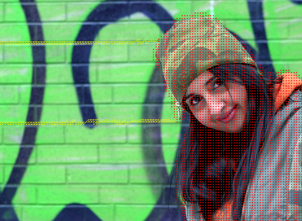
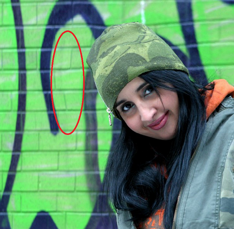
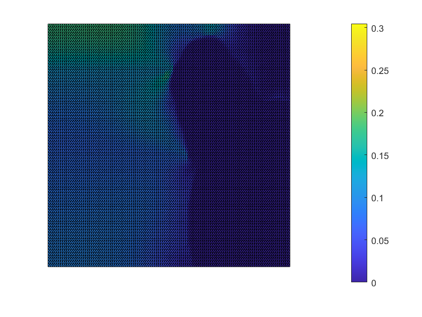
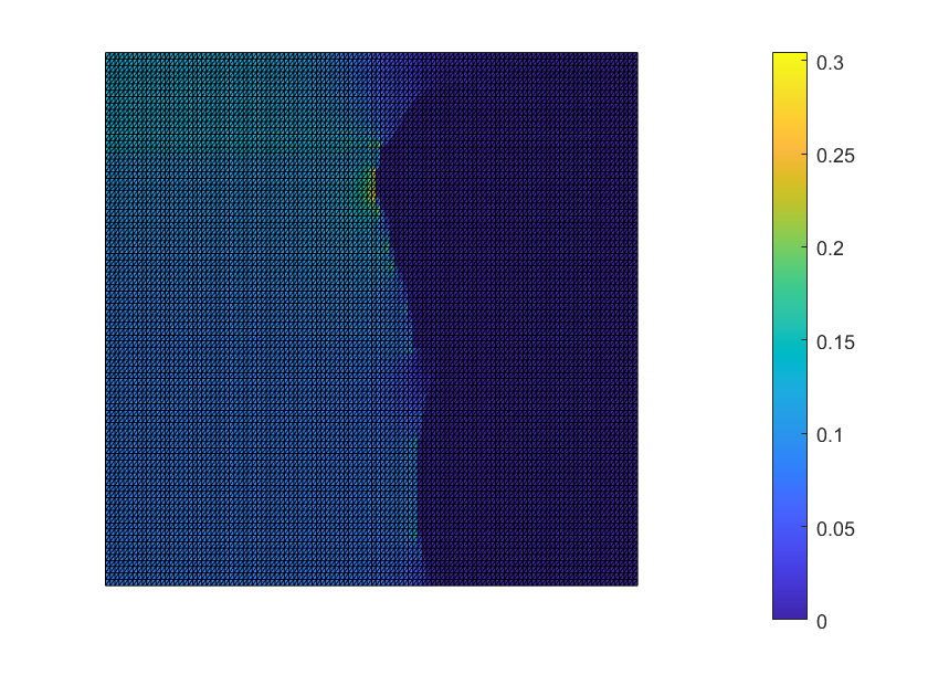
We have tested the proposed algorithm on various images in the dataset[13]. The results show that our model can preserve ROIs and line structures in images while changing the local geometry of the object as little as possible. The critical step of our algorithm and image retargeting of Beltrami representation [8] is solving a linear system, so both of them can get the results in a short time. Then, we make a comparison with BR and our method on a girl image 2. The yellow parts are selected line structures and the region in red is the ROI in the image. We can find that though the maximum conformal energy density of our result is higher, the density distribution of our method is more even than the BR model. The conformal energy of our result is less than that of the BR method because of the conformal energy minimizer, which means more local geometric information is preserved. The brick joints in our result look more natural than the BR method, especially for vertical joints on the left side of the image (the portion highlighted in red).


We can also extend our algorithm into an automatic one. The saliency map can compute the importance score of every pixel in images. We choose those parts with the top 25% scores as our regions of interest (ROIs). Here, we give an example 3. It is shown by the example that our model can deal with the retargeting problem whose ratio is 0.5 very well.


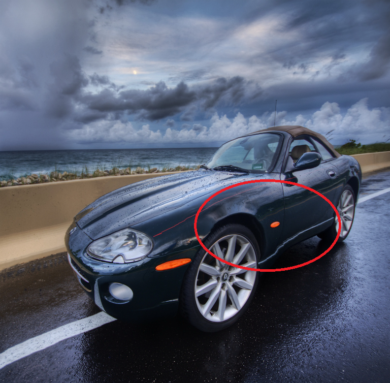
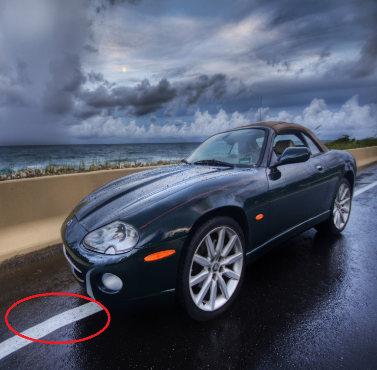
We compare our automatic method with several retargeting algorithms, including Simple scaling (SCL), Seam-Carving (SC, [14]), Nonhomogeneous warping (WARP, [16]), image retargeting algorithm via Beltrami representation (BR, [8]). OI represents the original image. The of our retargeting model in these experiments are all computed by the initialization method 17. The results are displayed in Figure 4-10. In Figure 4, the car in the results of the SCL method looks longer than the original one. Obvious distortion of line structures on the car in the SC model can be detected (circled in red). For the WARP model, the white line on the ground is turned into curves (circled in red). The results of the BR method and our method are similar, in which the car and line structures are well preserved. Taking Figure 6 as an example of images without important line structure, our output is satisfying while the tiger in the result of the SCL method looks thinner than the original one and the one in the result of the SC method looks fatter. We can also find that the performance of our algorithm depends on the proper selection of ROIs and line structures. The man in 9 is mapped to a small region in our result, and the reflection in our boat picture 10 looks unnatural because they are not selected as ROIs. These results also show the outstanding capacity for retargeting of our model in case of proper selection of ROIs and line structures.


6 Conclusions
In this paper, we have proposed an effective one-step image retargeting algorithm based on the conformal energy minimizer, which can preserve ROIs and the algorithm is robust and time-saving. It can also deal with large resizing ratio problems.
We talk about the conformal energy in this paper, but there is a gap for simplicial mapping approximation of quasi-conformal mapping because the corresponding matrix of is not an M-matrix on most meshes. Therefore, it is meaningful to do the research and find out what kind of mesh can be applied in quasi-conformal energy minimizing problems. Additionally, quasi-conformal mapping in higher dimensional space is a complex problem. Hopefully, we can give a good solution from the energy perspective to this problem.
The simplicial mapping approximation method can also solve the minimum curve surface problem. The area of is fixed in the image retargeting problem. While in the minimum curve surface problem, the area is not fixed, so the situation becomes much harder. We may further analyze the simplicial approximation convergence properties in that problem.
References
- [1] S. Avidan and A. Shamir, Seam carving for content-aware image resizing, ACM Transactions on Graphics (TOG), 26 (2007), pp. 10–es.
- [2] A. Berman and R. J. Plemmons, Nonnegative matrices in the mathematical sciences, SIAM, 1994.
- [3] M. Floater, One-to-one piecewise linear mappings over triangulations, Mathematics of Computation, 72 (2003), pp. 685–696.
- [4] X. D. Gu and S.-T. Yau, Computational conformal geometry, vol. 1, International Press Somerville, MA, 2008.
- [5] J. Harel, C. Koch, and P. Perona, Graph-based visual saliency, Advances in neural information processing systems, 19 (2006).
- [6] J. E. Hutchinson, Computing conformal maps and minimal surfaces, in Theoretical and Numerical Aspects of Geometric Variational Problems, vol. 26, Australian National University, Mathematical Sciences Institute, 1991, pp. 140–162.
- [7] L. Itti, C. Koch, and E. Niebur, A model of saliency-based visual attention for rapid scene analysis, IEEE Transactions on pattern analysis and machine intelligence, 20 (1998), pp. 1254–1259.
- [8] C. P. Lau, C. P. Yung, and L. M. Lui, Image retargeting via beltrami representation, IEEE Transactions on Image Processing, 27 (2018), pp. 5787–5801.
- [9] Y. Lipman, Bijective mappings of meshes with boundary and the degree in mesh processing, SIAM Journal on Imaging Sciences, 7 (2014), pp. 1263–1283.
- [10] J. J. Molitierno, Applications of combinatorial matrix theory to Laplacian matrices of graphs, CRC Press, 2016.
- [11] T. Ren, Y. Liu, and G. Wu, Image retargeting using multi-map constrained region warping, in Proceedings of the 17th ACM international conference on Multimedia, 2009, pp. 853–856.
- [12] C. P. Rourke and B. J. Sanderson, Introduction to piecewise-linear topology, Springer Science & Business Media, 2012.
- [13] M. Rubinstein, D. Gutierrez, O. Sorkine, and A. Shamir, A comparative study of image retargeting, in ACM SIGGRAPH Asia 2010 papers, 2010, pp. 1–10.
- [14] M. Rubinstein, A. Shamir, and S. Avidan, Improved seam carving for video retargeting, ACM transactions on graphics (TOG), 27 (2008), pp. 1–9.
- [15] J. Van Schaftingen, Approximation in sobolev spaces by piecewise affine interpolation, Journal of Mathematical Analysis and Applications, 420 (2014), pp. 40–47.
- [16] L. Wolf, M. Guttmann, and D. Cohen-Or, Non-homogeneous content-driven video-retargeting, in 2007 IEEE 11th international conference on computer vision, IEEE, 2007, pp. 1–6.
- [17] J. Xu, H. Kang, and F. Chen, Content-aware image resizing using quasi-conformal mapping, The Visual Computer, 34 (2018), pp. 431–442.
- [18] M.-H. Yueh, W.-W. Lin, C.-T. Wu, and S.-T. Yau, An efficient energy minimization for conformal parameterizations, Journal of Scientific Computing, 73 (2017), pp. 203–227.