Tensor Network Space-Time Spectral Collocation Method for Time Dependent Convection-Diffusion-Reaction Equations

Abstract

Emerging tensor network techniques for solutions of Partial Differential Equations (PDEs), known for their ability to break the curse of dimensionality, deliver new mathematical methods for ultra-fast numerical solutions of high-dimensional problems. Here, we introduce a Tensor Train (TT) Chebyshev spectral collocation method, in both space and time, for solution of the time dependent convection-diffusion-reaction (CDR) equation with inhomogeneous boundary conditions, in Cartesian geometry. Previous methods for numerical solution of time dependent PDEs often use finite difference for time, and a spectral scheme for the spatial dimensions, which leads to slow linear convergence. Spectral collocation space-time methods show exponential convergence, however, for realistic problems they need to solve large four-dimensional systems. We overcome this difficulty by using a TT approach as its complexity only grows linearly with the number of dimensions. We show that our TT space-time Chebyshev spectral collocation method converges exponentially, when the solution of the CDR is smooth, and demonstrate that it leads to very high compression of linear operators from terabytes to kilobytes in TT-format, and tens of thousands times speedup when compared to full grid space-time spectral method. These advantages allow us to obtain the solutions at much higher resolutions.

1 Introduction

Solving realistic problem often require numerical solutions of high dimensional partial differential equations (PDEs). The discretization of these PDEs leads to a steep rise in the computational complexity in terms of storage and number of arithmetic operations with each added dimension, often rendering traditional numerical approaches impractical. This phenomenon, known as “the curse of dimensionality”, cf. [2], represents a formidable barrier to multidimensional numerical analysis, one that persists even in the era of exascale high-performance computing.

In recent years, tensor networks (TNs) [1] have come to the forefront as a promising strategy to counteract or circumvent the curse of dimensionality. TNs restructure high-dimensional data into networks of lower-dimensional tensors, enabling the division of complex data into more manageable subsets. Tensor factorizations such as the Canonical Polyadic Decomposition, Hierarchical Tucker decomposition [16], and Tensor Train decompostion [28] are example of tensor networks. Originally devised within the realm of theoretical physics, these methods now showcase their potential for accurate and efficient numerical solutions to high-dimensional PDEs.

Through a process we will term tensorization, tensor networks offer an innovative means to efficiently represent the key elements of numerical algorithms for PDEs: grid functions that capture function values at grid nodes, and discrete operators approximating differential operators. This methodology has been applied successfully to a variety of challenging equations, from the quantum mechanical to the classical continuum [15, 10, 3, 24, 21, 22, 37, 36, 17, 35].

The present work considers the time-dependent convection-diffusion-reaction (CDR) equation, a model equation of critical importance across a broad spectrum of physical and engineering systems. The CDR equation enables quantitative descriptions of heat transfer, mass transfer, fluid dynamics, and chemical interactions in complex settings from microscale processing to atmospheric modeling. Numerical methods for the multidimensional CDR equation also constitute a major research area given the equation’s utility spanning such a vast range of transport phenomena critical to climate modeling, energy systems, biomedical systems, materials synthesis, and related domains central to technology innovation [34, 4, 5].

Classical numerical methods, like finite differences and finite volumes, necessitate extremely fine grids for precision, leading to voluminous linear systems that are challenging to solve, particularly when the problem spans four dimensions (one temporal and three spatial). This is why spectral collocation methods are considered, due to their greater efficiency.

The spectral collocation method approximates the solution to convection-diffusion-reaction (CDR) equations through the use of high-degree polynomial interpolants, e.g., Legendre and Chebyshev. These interpolants are evaluated at specific collocation points chosen within the domain. Assuming that the groundtruth solution is regular enough, one of the most notable advantages of this approach is the exponential convergence, where the interpolation error decreases exponentially as the degree of the polynomial increases. As a computational method for solving partial differential equations (PDEs), spectral collocation offers several significant benefits, as highlighted by Funaro [9]: $(i)$, the method achieves a high level of precision due to its inherent exponential convergence as the number of degrees of freedom grows; $(ii)$, it accurately represents solutions that exhibit complex spatial variations by employing smooth and continuous basis functions; $(iii)$ the basis functions are globally defined over the entire domain, making the spectral collocation method particularly suitable at handling problems with non-local interactions and dependencies.

Yet, the standard procedure for time-dependent PDEs, which couples spectral discretization of spatial derivatives with low-order temporal derivatives, often results in a temporal error that overshadows the spatial precision. Ideally, the accuracy of time integration should align with that of the spatial spectral approximation. Recent advancements in this area aim to overcome the time-stepping limitations by integrating space-time spectral collocation methods, which have shown exponential convergence in both spatial and temporal dimensions for sufficiently smooth heat equation solutions [19].

Despite these advances, the curse of dimensionality remains a significant challenge for space-time spectral methods applied to CDR equations, as computational complexity grows exponentially with problem size. In this study, we explore the discretization of the CDR equation in both space and time, employing a space-time operator scheme that simultaneously addresses spatial and temporal dimensions. This approach is particularly effective for phenomena with rapid dynamic changes where spatial and temporal variations are closely linked [23]. Although the space-time method traditionally faces the drawback of increased computational cost and memory requirements, we will demonstrate that tensor network techniques effectively overcome these challenges.

We utilize spectral collocation discretization within this space-time framework, expanding the PDE solution in terms of a set of global basis functions. For the non-periodic CDR equation solution, we employ the Chebyshev polynomials as our basis functions. The Chebyshev collocation method requires regular grids, that is, it works mainly on Cartesian grids that are tensor products of 1-D domain partitions, which is suitable to our tensor network formats.

The outline of the paper is as follows. In Section 2.2, we review some basic concepts for space-time collocation methods, introduce the discretization and its matrix formulation that leads to a linear system. In Section 3, we review the tensor notations and definitions of the TT-format, and the TT-matrix format for linear operators. In Section 3.4, we present our TT design of the numerical solution of the CDR equation and introduce our algorithms in tensor train format. In Section 4, we present our numerical results and assess the performance of our method. In Section 5, we offer our final remarks and discusses possible future work. For completeness, part of the details of the CDR tensorization approach are in a final appendix.

2 Mathematical Model and Numerical Discretization

2.1 Convection-Diffusion-Reaction Equation

We are interested in the following CDR problem: Find $u(t,\mathbf{x})$ such that

$$\frac{\partial u}{\partial t}-\kappa(t,\mathbf{x})\Delta u+\mathbf{b}(t,\mathbf{x})\cdot\nabla u+c(t,\mathbf{x})u =f(t,\mathbf{x})\phantom{g(t,\mathbf{x})h(\mathbf{x})}\text{in}\ (0,T]\times\Omega,$$

$$u =g(t,\mathbf{x})\phantom{f(t,\mathbf{x})h(\mathbf{x})}\text{on}\ [0,T]\times\partial\Omega,$$ (2.1)

$$u(0,\mathbf{x}) =h(\mathbf{x})\phantom{f(t,\mathbf{x})g(t,\mathbf{x})}\text{in}\ \Omega,$$

where $\kappa(t,\mathbb{x})$, $\vec{b}(t,\mathbb{x})$, and $c(t,\mathbf{x})$ are the diffusion, convection and reaction coefficients, respectively. Furthermore, $\Omega\subset\mathbb{R}^{3}$ be a three dimensional, open parallelepipied domain with boundary $\partial\Omega$; $h(\mathbb{x})$ is the initial condition, (IC), and $g(t,\mathbb{x})$ are the boundary conditions (BC). Here we denote the 3D vectors, such as, $\vec{x}=(x,y,z)$, and matrices, in bold font.

2.2 Chebyshev collocation method

We expand the approximate solution of the CDR equation on the set of orthogonal Chebyshev polynomials $T_{k}(x)$ = cos(k*arcos(x)) as global basis functions. Then, we enforce the CDR equation at a discrete set of points within the domain, known as collocation points, leading to a system of equations for the unknown expansion coefficients that we can solve. The collocation points of the Chebyshev grid are defined as in [14], and form the so-called collocation grid, cf. [9]. To this end, we need expressions for the derivatives of the approximate solution on the Chebyshev grid. The derivative expansion coefficients with respect to the same set of Chebyshev polynomials are determined by multiplying the matrix representation of the partial differential operators and the expansion coefficients of the numerical solution. In the rest of this section, we construct the time derivative, ${\partial}/{\partial t}$, the gradient, $\nabla$, and the Laplacian, $\Delta$. To simplify such matrix representations, we modify the Chebyshev polynomials (following Ref. [9]), and construct a new set of $N$-th degree polynomials $l_{j}$, $0\leq j\leq N$, with respect to the collocation points, $x_{i}$, $0\leq i\leq N$, that satisfy:

$$l_{j}(x_{i})=\left\{\begin{aligned} &1\qquad\text{if }\ i=j,\\ &0\qquad\text{if }\ i\neq j.\end{aligned}\right.$$ (2.2)

Using the new polynomials $l_{j}$, the discrete CDR solution becomes,

$$u_{h}(x):=\sum_{j=0}^{N}u(x_{j})l_{j}(x).$$ (2.3)

We construct all the spatial partial differential operators using the matrix representation of the single, one-dimensional derivative, $\mathbb{S}_{x}$, which reads as

$$\left(\frac{\partial}{\partial x}\right)_{ij}\rightarrow(\mathbb{S}_{x})_{ij}:=\frac{d}{dx}l_{j}(x)\Big{|}_{x_{i}}.$$ (2.4)

The size of the matrix $\mathbb{S}_{x}$ is $(N+1)\times(N+1)$. We obtain the second order derivative matrix, $\mathbb{S}_{xx}$, by matrix multiplication of the first order derivatives as,

$$(\mathbb{S}_{xx})_{ij}=\sum_{s=0}^{N}(\mathbb{S}_{x})_{is}(\mathbb{S}_{x})_{sj}.$$ (2.5)

For completeness, we refer to [9] for the derivation of this expression.

2.2.1 Matrix form of the discrete CDR equation

First, we introduce the space-time matrix operators: $\frac{\partial}{\partial t}\rightarrow$ $\mathbb{A}_{t}$; $\kappa(t,\mathbb{x})\Delta$ $\rightarrow$ $\mathbb{A}_{D}$; $\mathbf{b}(t,\mathbb{x})\cdot\nabla$ $\rightarrow$ $\mathbb{A}_{C}$; and $c(t,\mathbb{x})$ $\rightarrow$ $\mathbb{A}_{R}$, respectively. Upon employing these matrices, Eq.(2.1) results in the following linear system,

$$(\mathbb{A}_{t}+\mathbb{A}_{D}+\mathbb{A}_{C}+\mathbb{A}_{R})\mathbb{U}=\mathbb{F},$$ (2.6)

where $\mathbb{U}$, and $\mathbb{F}$ are the vectors corresponding to the solution, $u_{h}(t,\mathbb{x})$, and the loading term $f(t,\mathbb{x})$, respectively. The matrices $\mathbb{A}_{t}$, $\mathbb{A}_{D}$, $\mathbb{A}_{C}$, and $\mathbb{A}_{R}$ are of size $(N+1)^{4}\times(N+1)^{4}$ for $N^{th}$ order spectral collocation method, while $\mathbb{U}$, $\mathbb{F}$ are column vectors of size $(N+1)^{4}\times 1$, and are designed to incorporate the boundary conditions in Eq.(2.1).

2.2.2 Time discretization using finite differences and Chebyshev grids

Here, we display two strategies to discretize the first-order derivative with respect to the time variable. First, we present the well-known temporal finite difference approach with the implicit backward Euler method [18], and second we introduce a temporal spectral collocation discretization on a temporal Chebyshev grid. In both strategies the space operators are discretized on a spatial Chebyshev grid.

$\bullet$ Finite difference approach: With $N+1$ time points, $t_{0},t_{1},\ldots,t_{N}$, such that $t_{0}=0$ and $t_{N}=T$ are the initial and final time points, the length of the time step is $\Delta t=(T-T_{0})/N$. We emphasize that the backward Euler method is unconditionally stable and thus the stability is independent of the size of the time-step $\Delta t$ [18]. To consider the finite differences approach, we need to represent space and time separately. For this purpose we introduce a separate representation of the column vector, $\mathbb{U}$, as a column vector with $(N+1)$ components, each of size $(N+1)^{3}\times 1$: $\mathbb{U}^{T}=[\mathbb{\hat{U}}_{0}^{T},\ldots,\mathbb{\hat{U}}_{{N}}^{T}]$. Each component $\mathbb{\hat{U}}_{k}$, represents the spatial part of the solution at time point $t_{k}$. Let $\mathbb{\hat{F}}_{k}$ represent the load vector at time point $t_{k}$. In the temporal finite difference approach, at each time step we have to solve the following linear system,

$$\Big{(}\mathbb{I_{\text{space}}}+\Delta t\mathbb{S}_{\text{space}}\Big{)}\mathbb{\hat{U}}_{k+1}=\mathbb{\hat{U}}_{k}+\Delta t\mathbb{\hat{F}}_{k+1},\quad k=0,\ldots,N.$$ (2.7)

Here, $\mathbb{I_{\text{space}}}$ is the space-identity matrix of size $(N+1)^{3}\times(N+1)^{3}$, and, $\mathbb{S}_{\text{space}}$ = $\mathbb{A}_{D}$+$\mathbb{A}_{C}$+$\mathbb{A}_{R}$, is the space spectral matrix which is positive definite. Hence, we have, $\text{det}(\mathbb{I_{\text{space}}}+\Delta t\mathbb{S}_{\text{space}})\neq 0$, and the linear system Eq. (2.7) has a unique solution. We can unite the space and time operators and solve Eq. (2.7) in a single step. First, we rewrite Eq. (2.7) as follows:

$$\frac{1}{\Delta t}\mathbb{\hat{U}}_{k+1}-\frac{1}{\Delta t}\mathbb{\hat{U}}_{k}+\mathbb{S}_{\text{space}}\mathbb{\hat{U}}_{k+1}=\mathbb{\hat{F}}_{k+1}.$$ (2.8)

Then we define the time derivatives matrix, $\mathbb{T}$, consistent with the backward Euler scheme,

$$\mathbb{T}=\frac{1}{\Delta t}\begin{pmatrix}1&0&0&\cdots&0&0\\ -1&1&0&\cdots&0&0\\ 0&-1&1&\ldots&0&0\\ \vdots&\vdots&\vdots&\ddots&\vdots&\vdots\\ 0&0&0&\cdots&-1&1\end{pmatrix}_{(N+1)\times(N+1)}.$$ (2.9)

By employing $\mathbb{T}$, $\mathbb{S}_{\text{space}}$, and the Kronecker product, $\otimes$, we can construct the matricization of the space-time operator, $\mathbb{T}\otimes\mathbb{I}_{\text{space}}+\mathbb{I}_{t}\otimes\mathbb{S}_{\text{space}}$, where $\mathbb{I}_{t}$ is the time-identity matrix of size $(N+1)\times(N+1)$. Hence, the linear system, in the finite differences approach is:

$$(\mathbb{T}\otimes\mathbb{I}_{\text{space}}+\mathbb{I}_{t}\otimes\mathbb{S}_{\text{space}})\mathbb{U}=\mathbb{F}.$$ (2.10)

We note that in Ref. [7], the authors have employed the same finite difference technique to solve the heat equation in TT format.

$\bullet$ Time discretization on Chebyshev grid: When the order of the Chebyshev polynomials, $N\rightarrow\infty$, the PDE approximate solution, $u_{h}(t_{n},\mathbb{x})$, at time $t=t_{n}$ converges exponentially in space, as $N^{-|\alpha|}$ [9, Appendix A.4], and linearly with time step $\Delta t$,

$$\|u(t_{n},\mathbb{x})-u_{h}(t_{n},\mathbb{x})\|_{L^{2}(\Omega)}\leq(\Delta t+N^{-|\alpha|})\Big{\|}\frac{d^{|\alpha|}u(t_{n},\mathbb{x})}{d\mathbb{x}^{|\alpha|}}\Big{\|}_{L^{2}(0,T;L^{2}(\Omega))},$$ (2.11)

where $\frac{d^{|\alpha|}u(t,\mathbb{x})}{d\mathbb{x}^{|\alpha|}}\in L^{2}(\Omega)$, and $u(t,\mathbb{x})\in C^{0}(\Omega)$ for all $t\in(0,T)$. Here, $\alpha=(\alpha_{1},\alpha_{2},\alpha_{3})$ is a multi-index, which characterizes the smoothness of the CDR solution in space by $|\alpha|:=\alpha_{1}+\alpha_{2}+\alpha_{3}$. It can be seen that even for higher order Chebyshev polynomials, the global error is dominated by the error introduced by the temporal scheme that remains linear, which is the primary drawback of the temporal finite difference approach. To recover global exponential convergence, we apply Chebyshev spectral collocation method for discretization of both space and time variables. To accomplish this, we construct a single one-dimensional differential operator, $\frac{\partial}{\partial t}$ in matrix form, $(\mathbb{S}_{t})_{ij}$, on temporal Chebyshev grid, with collocation points $t_{0},t_{1}\ldots,t_{N}$, as follows (see Eq.(2.4)).

$$(\mathbb{S}_{t})_{ij}=\frac{dl_{j}(t)}{dt}\Big{|}_{t_{i}},\quad 0\leq i,j\leq N.$$ (2.12)

Hence, the linear system, in the space-time collocation method is,

$$(\mathbb{S}_{t}\otimes\mathbb{I}_{\text{space}}+\mathbb{I}_{t}\otimes\mathbb{S}_{\text{space}})\mathbb{U}=\mathbb{F},$$ (2.13)

where (see Eq. 2.6) $\mathbf{A}_{t}=\mathbb{S}_{t}\otimes\mathbb{I}_{\text{space}}$. To construct the space-time operator of the CDR equation on the Chebyshev grid we also need to construct the space part, $\mathbb{S}_{\text{space}}$.

2.2.3 Space discretization on Chebyshev grids

$\bullet$ Diffusion Operator on Chebyshev grid: In this section, we focus on the matricization of the diffusion term, $\kappa(t,\mathbb{x})\Delta$ $\rightarrow$ $\mathbb{A}_{D}$. The diffusion operator $\Delta$ is constructed as follows,

$$\begin{split}\Delta=\mathbb{I}_{t}\otimes\mathbb{S}_{xx}\otimes\mathbb{I}_{y}\otimes\mathbb{I}_{z}+\mathbb{I}_{t}\otimes\mathbb{I}_{x}\otimes\mathbb{S}_{yy}\otimes\mathbb{I}_{z}+\mathbb{I}_{t}\otimes\mathbb{I}_{x}\otimes\mathbb{I}_{y}\otimes\mathbb{S}_{zz}.\end{split}$$ (2.14)

Then, the function $\kappa(t,\mathbb{x})$ is incorporated to form the diffusion term $\mathbb{A}_{D}$

$$\mathbb{A}_{D}=diag(\boldsymbol{K})\Delta,$$ (2.15)

where $diag({\ldots})$ denotes a diagonal matrix, and ${\boldsymbol{K}}$ is a vector of size $(N+1)^{4}$ containing the evaluation of $\kappa(t,\mathbb{x})$ on the Chebyshev space-time grid.

$\bullet$ Discretization of the convection term on Chebyshev grid: Here, we focus on the matricization of the convection term, $\mathbf{b}(t,\mathbb{x})\cdot\nabla\rightarrow\mathbb{A}_{C}$, with the convective function, $\mathbf{b}(t,x,y,z)$, which we assume in the form

$$\mathbf{b}(t,x,y,z)=[b^{x}(t,x,y,z)~{}b^{y}(t,x,y,z)~{}b^{z}(t,x,y,z)].$$ (2.16)

Then, we construct the convection term $\mathbb{A}_{C}$

$$\begin{split}\mathbb{A}_{C}=\ &diag(\mathbb{B}^{x})\left(\mathbb{I}_{t}\otimes\mathbb{S}_{x}\otimes\mathbb{I}_{y}\otimes\mathbb{I}_{z}\right)+\ldots\\ &diag(\mathbb{B}^{y})\left(\mathbb{I}_{t}\otimes\mathbb{I}_{x}\otimes\mathbb{S}_{y}\otimes\mathbb{I}_{z}\right)+\ldots\\ &diag(\mathbb{B}^{z})\left(\mathbb{I}_{t}\otimes\mathbb{I}_{x}\otimes\mathbb{I}_{y}\otimes\mathbb{S}_{z}\right),\end{split}$$ (2.17)

where $\mathbb{B}^{x},\mathbb{B}^{y}$, and $\mathbb{B}^{z}$ are vectors of size $(N+1)^{4}$ containing the evaluation of the functions $b^{x},\ b^{y}$ and $b^{z}$ on the Chebyshev space-time grid.

$\bullet$ Discretization of the reaction term on Chebyshev grid: Here, we focus on the matricization of the reaction term, $c(t,\mathbb{x})$ $\rightarrow$ $\mathbb{A}_{R}$, which is given by $\mathbb{A}_{R}=diag(\mathbb{C})\mathbb{I}_{t}\otimes\mathbb{I}_{x}\otimes\mathbb{I}_{y}\otimes\mathbb{I}_{z}$, where $\mathbb{C}$ is the evaluation of the function $c(t,\mathbb{x})$ on the Chebyshev space-time grid.

2.2.4 Initial and boundary conditions on space-time Chebyshev grids

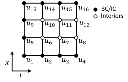
Figure 1: 1D Space time grid with $N=4$ collocation nodes.

So far, we have not incorporated the boundary conditions (BC) and the initial condition (IC), given in (2.1), into the linear system $\mathbb{A}\mathbb{U}=\mathbb{F}$ (2.13). In the space-time method, we consider the IC equivalent to the BC. The nodes of the Chebyshev grid are split into two parts: $(i)$ BC/IC nodes, and $(ii)$ interior nodes, where the solution is unknown. Let $i^{\text{Bd}}$, and $i^{\text{Int}}$ be the set of multi-indices, introduced in [6], the BC/IC and interior nodes, respectively.

Boundary and initial conditions are imposed by explicitly enforcing the BC/IC nodes to be equal to the BC, $g(t,x)$, or to the IC, $h(x)$, and then reducing the linear system for all nodes into a smaller system only for the interior nodes,

$$\mathbb{A}^{\text{Int}}\mathbb{U}^{\text{Int}}=\mathbb{F}^{\text{Int}}-\mathbb{F}^{\text{Bd}}.$$ (2.18)

To make it clear we consider below a simple example with $N=4$ collocation points in two dimensions $(t,x)$. The set of Chebyshev nodes can be denoted by multi-indices as, $\mathbb{U}:=\{u_{1},u_{2},\ldots,u_{16}\}$ (Figure 1). After imposing the BC/IC conditions, the linear system with BC/IC nodes, $\mathbb{A}\mathbb{U}=\mathbb{F}$, is

$$\begin{split}&u_{1}=g(t_{0},{x}_{0})\\ &\quad\vdots\\ &u_{4}=g(t_{3},{x}_{0})\\ &u_{5}=h(x_{1}),\\ &A_{6,1}u_{1}+A_{6,2}u_{2}+\ldots+A_{6,15}u_{15}+A_{6,16}u_{16}=F_{6}\\ &\quad\vdots\\ &A_{8,1}u_{1}+A_{8,2}u_{2}+\ldots+A_{8,15}u_{15}+A_{8,16}u_{16}=F_{8}\\ &u_{9}=h(x_{2})\\ &A_{10,1}u_{1}+A_{10,2}u_{2}+\ldots+A_{10,15}u_{15}+A_{10,16}u_{16}=F_{10}\\ &\quad\vdots\\ &A_{12,1}u_{1}+A_{12,2}u_{2}+\ldots+A_{12,15}u_{15}+A_{12,16}u_{16}=F_{12}\\ &\quad\vdots\\ &u_{13}=g(t_{0},{x}_{3})\\ &\quad\vdots\\ &u_{16}=g(t_{3},{x}_{3}).\\ \end{split}$$ (2.19)

The unknown values $(u_{6},u_{7},u_{8},u_{10},u_{11},u_{12})$ associated to six interior nodes, satisfy the reduced linear system whose equations read as

$$\qquad A_{l,6}u_{6}+A_{l,7}u_{7}+A_{l,8}u_{8}+A_{l,10}u_{10}+A_{l,11}u_{11}+A_{l,12}u_{12}\\ =F_{l}-A_{l,1}g(t_{0},x_{0})-A_{l,2}g(t_{1},x_{0})-\ldots,\qquad$$ (2.20)

with $l\in\{6,7,8,10,11,12\}$, where we transfer the values of BC/IC nodes to the right-hand side.

3 Tensor networks

In this section, we introduce the TT format, the specific tensor network we use in this work, the representation of linear operators in TT-matrix format, and the cross-interpolation method. All these methods are fundamental in the tensorization of our spectral collocation discretization of the CDR equation. For a more comprehensive understanding of notation and concepts, we refer the reader to the following references: Refs. [16, 28, 6], which provide detailed explanations.

3.1 Tensor train

The TT format, introduced by Oseledets in 2011 [28], represents a sequential chain of matrix products involving both two-dimensional matrices and three-dimensional tensors, referred to as TT-cores. We can visualize this chain as in Figure 2. Given that tensors in our formulation are at most four dimensional (one temporal and three spatial dimensions), we consider the tensor train format in the context of 4D tensors. Specifically, the TT approximation $\mathcal{X}^{TT}$ of a four-dimensional tensor $\mathcal{X}$ is a tensor with elements

$$\mathcal{X}^{TT}(i_{1},i_{2},i_{3},i_{4})=\sum^{r_{1}}_{\alpha_{1}=1}\sum^{r_{2}}_{\alpha_{2}=1}\sum^{r_{3}}_{\alpha_{3}=1}\mathcal{G}_{1}(1,i_{1},\alpha_{1})\mathcal{G}_{2}(\alpha_{1},i_{2},\alpha_{2})\mathcal{G}_{3}(\alpha_{2},i_{3},\alpha_{3})\mathcal{G}_{4}(\alpha_{3},i_{4},1)+\varepsilon,$$ (3.1)

where the error, $\varepsilon$, is a tensor with the same dimensions as $\mathcal{X}$, and the elements of the array $\mathbf{r}=[r_{1},r_{2},r_{3}]$ are the TT-ranks, and quantify the compression effectiveness of the TT approximation. Since, each TT core, $\mathcal{G}_{p}(i_{k})$, only depends on a single index of the full tensor $\mathcal{X}$, e.g., $i_{k}$, the TT format effectively embodies a discrete separation of variables [1].

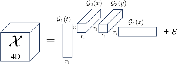
Figure 2: TT decomposition of a 4D tensor $\mathcal{X}$, with TT rank, $\mathbf{r}=\big{[}r_{1},r_{2},r_{3}\big{]}$, and approximation error $\varepsilon$, in accordance with Eq. (3.1).

In Figure 2 we show a four-dimensional array $\mathcal{X}(t,x,y,z)$, decomposed in TT-format.

3.2 Linear Operators in TT-matrix format

Suppose that the approximate solution of the CDR equation is a 4D tensor $\mathcal{U}$, then the linear operator $\mathcal{A}$ acting on that solution is represented as an 8D tensor. The transformation $\mathcal{A}\mathcal{U}$ is defined as:

$$\big{(}\mathcal{A}\mathcal{U}\big{)}(i_{1},i_{2},i_{3},i_{4})=\sum_{j_{1},j_{2},j_{3},j_{4}}\mathcal{A}(i_{1},j_{1},\dots,i_{4},j_{4})\mathcal{U}(j_{1},\dots,j_{4}).$$

The tensor $\mathcal{A}$ and the matrix operator $\mathbb{A}$, defined in Eq. (2.18), are related as:

$$\mathcal{A}(i_{1},j_{1},\dots,i_{4},j_{4})=\mathbb{A}(i_{1}i_{2}i_{3}i_{4},j_{1}j_{2}j_{3}j_{4}).$$ (3.2)

Thus, we can construct the tensor $\mathcal{A}$ by suitably reshaping and permuting the dimensions of the matrix $\mathbb{A}$. The linear operator, $\mathcal{A}$, can be further represented in a variant of TT format, called TT-matrix, cf. [35]. The component-wise TT-matrix $\mathcal{A}^{TT}$ is defined as:

$$\mathcal{A}^{TT}(i_{1},j_{1},\ldots,i_{4},j_{4})=\sum_{\alpha_{1},\alpha_{2},\alpha_{3}}\mathcal{G}_{1}\big{(}1,(i_{1},j_{1}),\alpha_{1}\big{)}\ldots\mathcal{G}_{4}\big{(}\alpha_{3},(i_{4},j_{4}),1\big{)},$$ (3.3)

where $\mathcal{G}_{k}$ are 4D TT-cores .

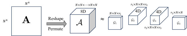
Figure 3: Representation of a linear matrix $\mathbf{A}$ in the TT-matrix format. First, we reshape the operation matrix $\mathbb{A}$ and permute its indices to create the tensor $\mathcal{A}$. Then, we factorize the tensor in the tensor-train matrix format according to Eq. (3.3) to obtain $\mathcal{A}^{\text{TT}{}}$.

Figure 3 shows the process of transforming a matrix operator $\mathbb{A}$ to its tensor format, $\mathcal{A}$, and, finally, to its TT-matrix format, $\mathcal{A}^{\text{TT}{}}$.

We can further simplify the TT-matrix representations of the matrix $\mathbb{A}$ if it is a Kronecker product of matrices, i.e. $\mathbb{A}=\mathbb{A}_{1}\otimes\mathbb{A}_{2}\otimes\mathbb{A}_{3}\otimes\mathbb{A}_{4}$. Based on the relationship defined in Eq. (3.2), the tensor $\mathcal{A}$ can be constructed using tensor product as $\mathcal{A}=\mathbb{A}_{1}\circ\mathbb{A}_{2}\circ\mathbb{A}_{3}\circ\mathbb{A}_{4}$. This implies the internal ranks of the TT-format of $\mathcal{A}$ in (3.3) are all equal to $1$. In such a case, all summations in Eq. (3.3) reduce to a sequence of single matrix-matrix multiplications, and the TT format of $\mathcal{A}$ becomes the tensor product of $d$ matrices:

$$\mathcal{A}^{TT} =\mathbf{A}_{1}\circ\mathbf{A}_{2}\circ\dots\circ\mathbf{A}_{d}.$$ (3.4)

This specific structure appears quite often in the matrix discretization, and will be exploited in the tensorization to construct efficient TT format.

3.3 TT Cross Interpolation

The original TT algorithm is based on consecutive applications of singular value decompositions (SVDs) on unfoldings of a tensor [28]. Although known for its efficiency, TT algorithm requires access to the full tensor, which is impractical and even impossible for extra-large tensors. To address this challenge, the cross interpolation algorithm, TT-cross, has been developed [27]. The idea behind TT-cross is essentially to replace the SVD in the TT algorithm with an approximate version of the skeleton/CUR decomposition [12, 20]. CUR decomposition approximates a matrix by selecting a few of its columns $\mathbf{C}$, a few of its rows $\mathbf{R}$, and a matrix $\mathbf{U}$ that connects them, as shown in Fig. 4. Mathematically, CUR decomposition finds an approximation for a matrix $\mathbf{A}$, as $\mathbf{A}\approx\mathbf{C}\mathbf{U}\mathbf{R}$. The TT-cross algorithm, utilizes the Maximum Volume Principle (maxvol algorithm) [11, 25] to determine $\mathbf{U}$. The maxvol algorithm chooses a few columns, $\mathbf{C}$ and rows, $\mathbf{R}$, of $\mathbf{A}$, such that, the intersection matrix $\mathbf{U}^{-1}$ has maximum volume [31].

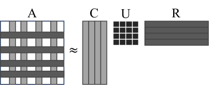
Figure 4: CUR decomposition

TT-cross interpolation and its versions can be seen as an heuristic generalization of CUR to tensors [30, 33]. TT-cross utilizes the maximum volume algorithm iteratively, often beginning with few randomly chosen fibers, to select an optimal number of specific tensor fibers that capture essential information of the tensor [32]. These fibers are used to construct a lower-rank TT representation. The naive generalization of CUR is proven to be expensive, which led to the development of various heuristic optimization techniques, such as, TT-ALS [13], DMRG [29, 31], and AMEN [8].

To solve the CDR equation, we use TT-cross to build the TT format, directly from the coefficient functions $\kappa(t,\mathbb{x})$, $\mathbb{b}(t,\mathbb{x})$, $c(t,\mathbb{x})$, boundary conditions, initial conditions, and loading functions.

3.4 Tensorization

The space-time discretization produces a linear system for all interior nodes as specified in Eq. (2.18). Here, we simplify the notation, and refer to this equation as $\mathbb{A}\mathbb{U}=\mathbb{F}-\mathbb{F}^{\text{Bd}}$.

Tensorization is a process of building the TT format of all components of this linear system

$$\mathbb{A}\mathbb{U}=\mathbb{F}-\mathbb{F}^{\text{Bd}}\rightarrow\mathcal{A}^{TT}\mathcal{U}^{TT}=\mathcal{F}^{TT}-\mathcal{F}^{\text{Bd},TT},$$ (3.5)

where $\mathcal{A}^{TT}=\mathcal{S}_{t}^{TT}+\mathcal{A}_{D}^{TT}+\mathcal{A}_{C}^{TT}+\mathcal{A}_{R}^{TT}$.

In the matrix form, the operator $\mathbb{A}=\mathbb{A}_{t}+\mathbb{A}_{D}+\mathbb{A}_{C}+\mathbb{A}_{R}$ is designed to act on the vectorized solution $\mathbb{U}$. In the full tensor format, the solution is kept in its original tensor form $\mathcal{U}$, which is a 4D tensor. Consequently, all the operators $\mathcal{A}_{t},\ \mathcal{A}_{D},\ \mathcal{A}_{C},\text{ and }\mathcal{A}_{R}$ are 8D tensors. Lastly, $\mathcal{F}$ and $\mathcal{F}^{\text{Bd}}$ are both 4D tensors. Here, given that these operators in their matrix form have Kronecker product structure, their TT format can be constructed by using component matrices as TT cores. To construct the tensor format of the operators acting on the interior nodes, we need to define some sets of indices:

$$\begin{split}&\mathcal{I}_{t}=1:N\ \text{index set for time variable},\\ &\mathcal{I}_{s}=1:(N-1)\ \text{index set for space variable}.\end{split}$$

$\bullet$ TT-matrix Time Operator, $\mathcal{A}^{TT}_{t}$: The temporal operator in TT-matrix format acting only on the interior nodes is constructed as:

$$\mathcal{A}^{TT}_{t}=\mathbb{S}_{t}(\mathcal{I}_{t},\mathcal{I}_{t})\circ\mathbb{I}_{N-1}\circ\mathbb{I}_{N-1}\circ\mathbb{I}_{N-1},$$ (3.6)

where $\mathbb{I}_{N-1}$ is the identity matrix of size $(N-1)\times(N-1)$.

$\bullet$ TT-matrix Diffusion Operator, $\mathcal{A}^{TT}_{D}$: The Laplace operator in TT-matrix format is constructed as:

$$\begin{split}\Delta^{TT}=\mathbb{I}_{N}\circ\mathbb{S}_{xx}(\mathcal{I}_{s},\mathcal{I}_{s})\circ\mathbb{I}_{N-1}\circ\mathbb{I}_{N-1}+&\mathbb{I}_{N}\circ\mathbb{I}_{N-1}\circ\mathbb{S}_{yy}(\mathcal{I}_{s},\mathcal{I}_{s})\circ\mathbb{I}_{N-1}\\ +&\mathbb{I}_{N}\circ\mathbb{I}_{N-1}\circ\mathbb{I}_{N-1}\circ\mathbb{S}_{zz}(\mathcal{I}_{s},\mathcal{I}_{s}).\end{split}$$ (3.7)

Hence, the Laplace operator is a sum of three linear operators in TT-matrix formats, which again is a TT-matrix. Further, we need to format the diffusion coefficient $\kappa(t,\mathbb{x})$ on the Chebyshev grid of interior nodes in TT format. To transform $\kappa(t,\textbf{x})\rightarrow\mathcal{K}^{TT}$, we applied the cross-interpolation technique described in Section 3.3. Finally, we need to transform $\mathcal{K}^{TT}$ in TT-matrix format to be able to multiply it with $\Delta^{TT}$. The transformation to TT $\rightarrow$ TT-matrix is given in Algorithm 1.

Data: $\tentt{K}$

Result: $\mathcal{K}^{op,TT}$

1 Get the cores $\left\{\mathcal{G}_{k}\right\}_{k=1,2,3,4}$ from $\tentt{K}$.

2 $\{r_{0}=1,r_{1},r_{2},r_{3},r_{4}=1\}$ are TT ranks.

3 $\{n_{1},n_{2},n_{3},n_{4}\}$ are tensor sizes.

4 for k = 1:4 do

       $\mathcal{G}new_{k}=zeros(r_{k-1},n_{k},n_{k},r_{k})$ // create a zero tensor core

5       for i=1:$r_{k-1}$ do

6             for j=1:$r_{k}$ do

7                   $\mathcal{G}new_{k}(i,:,:,j)=diag(\mathcal{G}_{k}(i,:,j))$

8            

9      

Build $\mathcal{K}^{op,TT}$ using $\{\mathcal{G}new_{k}\}$ as its cores.

Algorithm 1 Reformat TT, $\tentt{K}$, in TT-matrix format, $\mathcal{K}^{op,TT}$

$\bullet$ TT-matrix Convection Operator, $\mathcal{A}^{TT}_{C}$: The convection operator in TT-matrix format is constructed as:

$$\begin{split}\nabla^{TT}_{x}=\mathbb{I}^{N}\circ\mathbb{S}_{x}(\mathcal{I}_{s},\mathcal{I}_{s})\circ\mathbb{I}^{N-1}\circ\mathbb{I}^{N-1},\\[5.0pt] \nabla^{TT}_{y}=\mathbb{I}^{N}\circ\mathbb{I}^{N-1}\circ\mathbb{S}_{y}(\mathcal{I}_{s},\mathcal{I}_{s})\circ\mathbb{I}^{N-1},\\[5.0pt] \nabla^{TT}_{z}=\mathbb{I}^{N}\circ\mathbb{I}^{N-1}\circ\mathbb{I}^{N-1}\circ\mathbb{S}_{z}(\mathcal{I}_{s},\mathcal{I}_{s}).\\ \end{split}$$ (3.8)

Next, the tensor operators $\mathcal{B}^{op,TT}_{x}$, $\mathcal{B}^{op,TT}_{y}$ and $\mathcal{B}^{op,TT}_{z}$ are computed from the functions $b^{x},\ b^{y}$ and $b^{z}$ in the same way as being computed with $\kappa(t,\mathbb{x})$. Then the TT-matrix format of convection operator is constructed as:

$$\mathcal{A}_{C}^{TT}=\mathcal{B}_{x}^{op,TT}\nabla_{x}^{TT}+\mathcal{B}_{y}^{op,TT}\nabla_{y}^{TT}+\mathcal{B}_{z}^{op,TT}\nabla_{z}^{TT}.$$ (3.9)

$\bullet$ TT-matrix Reaction Operator, $\mathcal{A}^{TT}_{R}$: The reaction operator $\mathcal{A}^{TT}_{R}$ basically is the function $c(t,\mathbb{x})$ being converted to an operator in the same way as with other coefficient functions.

Then the TT-matrix format of the operator $\mathcal{A}$ is constructed as

$$\mathcal{A}^{TT}=\mathcal{A}^{TT}_{t}+\mathcal{A}^{TT}_{D}+\mathcal{A}^{TT}_{C}+\mathcal{A}^{TT}_{R}.$$

$\bullet$ TT-matrix Loading Tensor, $\mathcal{F}^{TT}$: The TT-matrix loading tensor $\mathcal{F}^{TT}$ is constructed by applying the cross interpolation on the function $f(t,\mathbb{x})$ on the grid of interior nodes.

$\bullet$ TT Boundary Tensor, $\mathcal{F}^{Bd,TT}$: The boundary tensor $\mathcal{F}^{Bd}$ is used to incorporate the information about boundary and initial conditions into the linear system of the interior nodes. Only in the case of homogeneous BC and zero IC, this tensor is a zero tensor. Basically, the idea is to construct an operator $\mathcal{A}^{map}$, similar to $\mathcal{A}$. The difference is that $\mathcal{A}^{map}$ will be a mapping from all nodes to only unknown nodes. The size of the operator $\mathcal{A}^{map}$ is $N\times(N+1)\times(N-1)\times(N+1)\times(N-1)\times(N+1)\times(N-1)\times(N+1)$. Then, the boundary tensor $\mathcal{F}^{Bd}$ is computed by apply $\mathcal{A}^{map}$ to a tensor $\mathcal{G}^{Bd}$ containing only the information from BC/IC. The details about constructing $\mathcal{A}^{map,TT}$ and $\mathcal{G}^{Bd,TT}$ are included in the Appendix B.

At this point, we have completed constructing the TT-format of the linear system $\mathcal{A}^{TT}\mathcal{U}^{TT}=\mathcal{F}^{TT}-\mathcal{F}^{Bd,TT}$. To solve the TT linear system by optimization techniques, we used the routines amen_cross, amen_solve and amen_mm form the MATLAB TT-Toolbox [26].

4 Numerical Results

We investigate the computational efficiency and potential low-rank structures of the space-time solver by implementing the space-time operator in the tensor train format. To validate the algorithm presented earlier and assess its performance, we conducted several numerical experiments using MATLAB R2022b on a 2019 Macbook Pro 16 equipped with a 2.4 GHz 8-core i9 CPU. All our implementations rely on the MATLAB TT-Toolbox [26]. In the first example, we consider a manufactured solution of the time-dependent CDR equation with constant coefficients. The second example involves the space-time solution operator with non-constant coefficients. Finally, the third example showcases the behavior of the methods applied to the CDR with a non-smooth manufactured solution.

For all the examples, we compare the TT format of the space-time operator with the Finite Difference-Finite Difference (FD-FD) method and the Spectral-Spectral (SP-SP) collocation method. Additionally, we compared the TT format of SP-SP with the full grid formulation of the SP-SP method. To quantify the compression achieved, we introduced the compression ratio CR, defined as:

$$\mbox{\text{CR}}:=\frac{\mbox{\text{Mem}}(\mathcal{X}^{\text{TT}})}{\mbox{\text{Mem}}(\mathcal{X})},$$ (4.1)

where $\mbox{\text{Mem}}(\mathcal{X}^{TT})$ and $\mbox{\text{Mem}}(\mathcal{X})$ are the total memory required for storing the scheme’s unknows in the TT format, e.g., $\mathcal{X}^{\text{TT}}$ and the full tensor format, e.g., $\mathcal{X}$. We will show that the TT format may achieve significant compression of spectral-collocation differential operators from terabyte sizes to megabytes and even kilobytes when solving the CDR equation on very fine meshes. Such a compression especially reduces the memory requirements for solving the linear system that results from the CDR equation discretization.

4.1 Test 1: Manufactured Solution with Constant Coefficients

In this first test, we study the convergence behavior of the benchmark problem described by Eq. (2.1) on the computational domain $[0,1]\times[-50,50]^{3}$. We consider constant coefficients, specifically $\kappa(t,\mathbb{x})=1$, $\mathbb{b}(t,\mathbb{x})=(1,1,1)$, and $c(t,\mathbb{x})=1$. The right-hand side force function $f(t,\mathbb{x})$ and the boundary conditions are determined in accordance with the exact solution $u(t,x,y,z):=\sin(2\pi(t+x+y+z))$.

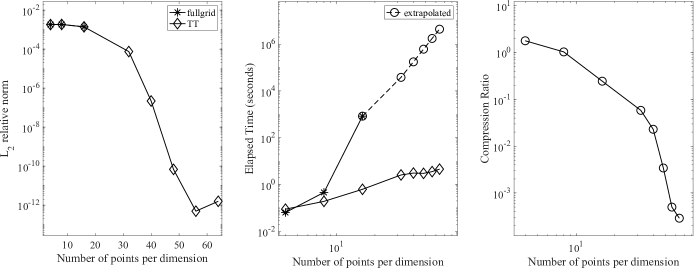
Figure 5: Test 1: Left Panel: Relative error curve in $L^{2}$ norm showing the exponential convergence of SP-SP schemes. Middle Panel: Elapsed time in seconds. Right Panel: Compression ratio of the solution. All plots are versus the number of points per dimension.

Figure 5 presents the results of this test. The left panel displays the relative error curve in the $L^{2}$ norm, demonstrating the exponential convergence of the SP-SP schemes. The middle panel depicts the elapsed time in seconds, indicating that the TT format enables solutions with much higher resolution compared to the full grid format. The right panel illustrates the compression ratio of the solution. We plot all curves against the number of points per dimension.

In Figure 5, we compare the SP-SP method in the full grid format and the SP-SP method in TT format. In the left panel, we plot the $L^{2}$ relative norms computed using the full grid and TT format against the number of nodes per dimension. The TT format provides the same level of accuracy as the full grid scheme. However, the TT format allows us to handle large data sets, unlike the full grid approach, which is limited to small grid data. This characteristic ensures that the TT format utilizes significantly less memory than the full-grid approach, making handling large data sets practical. Furthermore, the numerical results demonstrate the well-known exponential convergence of the spectral method. In the full grid computation, we achieve an accuracy of approximately $10^{-3}$, while in the TT format, we attain an accuracy of approximately $10^{-12}$ with only a minimal increase in grid data. At 64 nodes, the accuracy does not improve further as it reaches the truncation tolerance of the TT format.

In the middle panel, we compare the elapsed time (in seconds) required for both the TT format and full grid approaches. In the TT format, the elapsed time to compute the space-time operator increases linearly while preserving the invariance of the variables. On the other hand, in the full grid approach, the elapsed time increases exponentially. This behavior aligns with the theoretical prediction as the complexity grows linearly. For instance, with 16 nodes per dimension, the time taken in the TT format (represented by the third cross point) is 1400 times faster than in the full grid format (represented by the circled point).

Finally, we emphasize that this speed-up will further improve for larger grids. For example, based on the extrapolated elapsed time for the full grid scheme, we expect the TT method to be approximately $9\times 10^{5}$ times faster with 64 nodes per dimension.

Another interesting aspect is the compression ratio, which we defined in Eq. (4.1). In the right panel of Figure 5, we present the plot of the compression ratio versus the number of nodes per dimension, indicated by the curve. The compression ratio exponentially decreases as the number of nodes per dimension increases. At $64$ nodes per dimension, we achieve a compression ratio that saves approximately $10^{4}$ orders of magnitude in storage. This remarkable reduction in storage requirements is further illustrated in Table 1, where we showcase the compression of the aggregated operator $\mathcal{A}$, which is the memory bottleneck of the full grid scheme. The TT format allows full utilization of terabyte-sized operators while utilizing only kilobytes of storage. These results demonstrate the computational advantages of the SP-SP scheme in TT format compared to existing techniques.

Number of points per dimension	size of $\mathcal{A}$ in TB	size of $\mathcal{A}^{TT}$ in KB	Compress ratio
8	1.66e-5	3.58e0	2.00e-4
16	1.23e-2	1.88e1	1.42e-6
32	5.10e0	8.53e1	1.56e-8
64	1.64e3	3.63e2	2.06e-10

Table 1: Storage cost comparison of $\mathcal{A}$ between full-format and TT-format formulations. At $64$ points, the TT-format allows a compression from $1640$ Tb to $363$ Kb, which is about ten orders of magnitude.

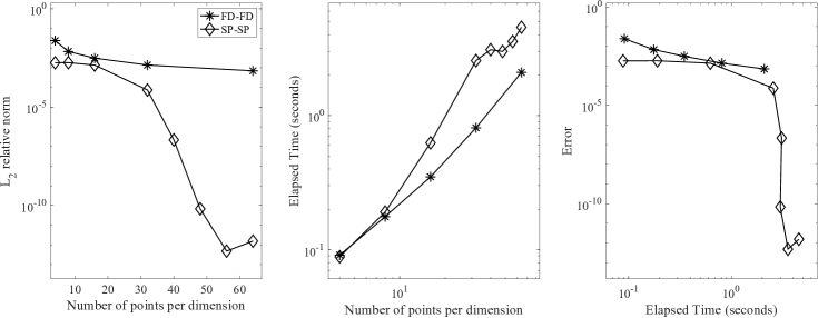
Figure 6: Test 1: Comparison between TT SP-SP and TT FD-FD. Left Panel: Plot of relative error versus number of points per dimension. Middle Panel: Plot of elapsed time versus number of points per dimension. Right Panel: Plot of relative error versus elapsed times, which shows that the TT SP-SP is more efficient compared to TT FD-FD.

Next, we aim to compare the performance of the SP-SP scheme with the FD-FD scheme, both in TT format. The space-time FD-FD scheme was initially proposed by Dolgov et al. [7]. In Fig. 6, we compare the SP-SP scheme in TT format and the FD-FD scheme in TT format. The left panel shows the $L^{2}$ relative error norms computed by both schemes in TT format. As the SP-SP scheme converges exponentially, it provides significantly more accurate results than the FD-FD scheme, which converges linearly. For instance, at $64$ nodes per dimension, the approximation error of the SP-SP scheme is approximately $10^{-11}$, while the approximation error of the FD-FD scheme is only of the order of $10^{-3}$. This fact shows that our TT-based spectral-collocation method is approximately $10^{-8}$ times more accurate than the FD-FD-based for the same grid data.

In the middle panel, we plot the elapsed time (in seconds) against the number of nodes per dimension. At $64$ nodes per dimension, the SP-SP scheme takes roughly twice as long as the FD-FD scheme. This indicates that the SP-SP scheme is slower by a factor of two compared to the FD-FD scheme. However, in the right panel, we observe that the SP-SP scheme computes highly accurate solutions relative to the consumed time, in contrast to the FD-FD scheme. Specifically, the SP-SP scheme requires $10$ seconds to compute a solution accurate to the order of $10^{-12}$, whereas the FD-FD scheme computes a solution accurate to the order of $10^{-3}$ within the same time frame.

In conclusion, we find that the SP-SP scheme computes highly accurate approximate solutions compared to existing techniques, such as the FD-FD scheme.

4.2 Test 2: Manufactured Solution with variable coefficients

In this test case, we examine the same model problem as above with the variable coefficients $\kappa(t,\mathbb{x})=\exp(-t^{2})$, $\mathbb{b}(t,\mathbb{x})=(\sin(2\pi x),\cos(2\pi y),\sin(2\pi z))$, and $c(t,\mathbb{x})=\cos(2\pi(t+x+y+z))$.

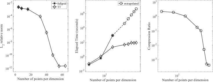
Figure 7: Test 2. Left Panel: Relative error curve in $L^{2}$ norm showing the exponential convergence of SP-SP schemes. Middle Panel: Elapsed time in seconds. TT format allows solutions in much higher resolution compared to the full grid format. Right Panel: Compression ratio of the solution. All plots are versus the number of points per dimension.

In Figure 7, we compare the TT format and the full grid approaches, where we use SP-SP in both cases. The TT approximation achieves the same level of accuracy as the full grid computation. The left panel plot illustrates the exponential convergence observed in both approaches. The error at $64$ nodes does not improve further because it reaches the truncation tolerance of the TT format.

In the middle panel, we compare the elapsed time (in seconds) required for both approaches. The time taken by the full grid approach increases exponentially, while it increases linearly in the TT format. We conclude that the TT format provides approximately a $40$-fold speed-up compared to the full grid computation at a grid size of $16$ nodes per dimension, and an estimated $5\times 10^{4}$ times faster at $64$ nodes based on extrapolated full grid time. It is worth noting that the full grid computation is unable to handle the grid data with 32 nodes per dimension due to memory limitations.

In the third panel, we show the compression ratio of the TT format against the number of nodes per dimension. As expected, the compression ratio decreases exponentially. It is significant to highlight that the SP-SP scheme with TT format achieves storage savings of approximately $10^{3}$ orders of magnitude at $64$ nodes per dimension. Additionally, Table 2 showcases the aggregated operator $\mathcal{A}$ compression, demonstrating that the TT format allows full access to terabyte-sized operators using only kilobytes of storage. For example, at $64$ nodes, the TT format only requires 1.81 MB of storage to store a full grid operator with a size of 1640 terabytes.

Number of points per dimension	size of $\mathcal{A}$ in TB	size of $\mathcal{A}^{TT}$ in KB	Compress ratio
8	1.66e-5	1.74e1	9.73e-4
16	1.23e-2	9.30e1	7.03e-6
32	5.10e0	4.24e2	7.75e-8
64	1.64e3	1.81e3	1.03e-9

Table 2: Storage Cost Comparison of $\mathcal{A}$ between full size and TT-format. At 64 points, the TT-format allows compression from 1640 TBs to about 1.81 MBs, which is about nine orders of magnitude.

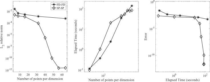
Figure 8: Test 2: Comparison between TT SP-SP and TT FD-FD. Left Panel: Relative error versus number of points per dimension. Middle Panel: Elapsed time versus number of points per dimension. Right Panel: Relative error versus elapsed times, which shows that the TT SP-SP is more efficient compared to TT FD-FD.

In Figure 8, we present a comparison between the FD-FD scheme in TT format and the SP-SP scheme in TT format. The left panel displays the plot of $L^{2}$ relative errors against the number of nodes per dimension. The SP-SP scheme with TT format achieves an approximation of the numerical solution that is approximately accurate to the order of $10^{-12}$, while the FD-FD scheme is only accurate to the order of $10^{-3}$ at 64 nodes per dimension.

In the middle panel, we plot the elapsed times for both methods against the number of nodes per dimension. Both methods consume almost the same amount of time for all grid data.

In the right panel, we plot the errors computed by both methods against the elapsed time. The SP-SP scheme generates a highly accurate numerical solution compared to the FD-FD scheme. Specifically, the SP-SP scheme achieves an accuracy of approximately $10^{-12}$, while the FD-FD scheme only approximates the solution to the order of $10^{-3}$ within the same time frame. Furthermore, the accuracy increases exponentially in the case of the SP-SP method.

4.3 Test 3: Non-smooth solution

The primary objective of this example is to validate the suitability of the tensor-train space-time spectral collocation method for solving the time-dependent CDR equation with less regular solutions. To investigate this aspect, we examine the behavior of the methods on a benchmark problem with the constant coefficients $\kappa(t,\mathbb{x})=1$, $\mathbb{b}(t,\mathbb{x})=(1,1,1)$, and $c(t,\mathbb{x})=1$, and the non-smooth exact solution $u(t,x,y,z):=\sin(\pi x)\sin(\pi y)\sin(\pi z)+x^{2}|x|$. As in the previous cases, computational domain is $[0,1]\times[-1,1]^{3}$.

The exact solution $u$ satisfies $\frac{d^{2}u(t,\mathbb{x})}{d\mathbb{x}^{2}}\in H^{\alpha}(0,T;L^{2}(\Omega))$ and $\frac{d^{2}u(t,\mathbb{x})}{d\mathbb{x}^{2}}\in C^{0}(\Omega)$ for all $t\in(0,T)$ and $\alpha>0$. Accordingly, Theorem 2.11 implies that the discrete approximation converges quadratically.

Indeed, we observe such a convergence order is clear in the left panel of Fig. 9. Due to the lower regularity of the exact solution, a highly refined mesh is required to achieve high accuracy, which is only feasible with the TT format.

In the middle panel, the plot shows that the SP-SP method is approximately $3500$ times faster than the full-grid SP-SP method using $16$ nodes, and about $1\times 10^{7}$ times faster using $128$ nodes, this latter being extrapolated on the full-grid. The compression ratio is approximately $5\times 10^{-4}$. Since the coefficient functions are the same as in Test Case 1, the compression of the operators in this test case is similar to the ones shown in Table 1.

Fig. 10 compares the TT FD-FD and TT SP-SP methods. The TT SP-SP method exhibits linear convergence compared to TT FD-FD with smaller approximation errors. Furthermore, as the grid size increases, the TT SP-SP method requires more elapsed time. The right panel, which plots the error versus elapsed time, clearly shows that the TT SP-SP method remains more efficient than the TT FD-FD method for this test case with a less regular solution.

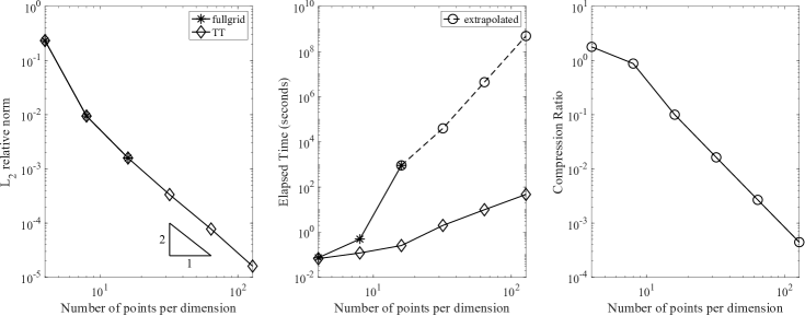
Figure 9: Test 3. Left Panel: Relative error curve in $L^{2}$ norm showing the linear convergence of SP-SP schemes, while the theoretical expected quadratic convergence is shown by the triangle. Middle Panel: Elapsed time in seconds. TT format allows solutions in much higher resolution compared to the full grid format. Right Panel: Compression ratio of the solution. All plots are versus the number of points per dimension.

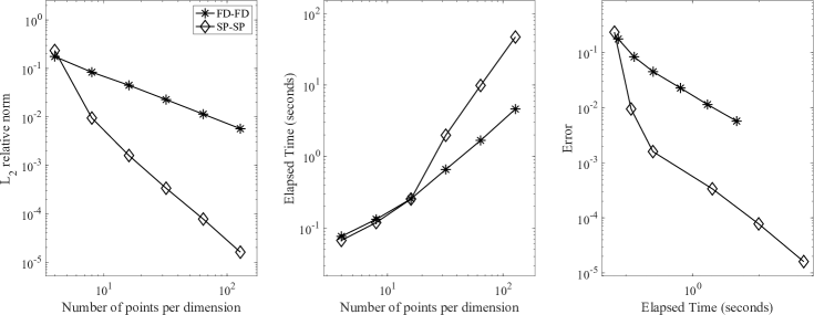
Figure 10: Test case-3:Comparison between TT SP-SP and TT FD-FD. Left Panel: Relative error versus number of points per dimension. Middle Panel: Elapsed time versus number of points per dimension. As the grid becomes larger, the TT SP-SP requires more computational time. Right Panel: Relative error versus elapsed times, which shows that the TT SP-SP is more efficient compared to TT FD-FD.

5 Conclusions

In this work, we introduce a method called the TT spectral collocation space-time (TT-SCST) approach for solving time-dependent convection-diffusion-reaction equations. Time is considered as an additional dimension, and the spectral collocation technique is applied in both space and time dimensions. This space-time approach demonstrates exponential convergence property for smooth functions. However, it involves solving a large linear system for solutions at all time points. Utilizing the tensorization process, we convert the linear system into TT-format and subsequently solve the TT linear system. Our numerical experiments validate that the TT-SCST method achieves significant compression of terabyte-sized matrices to kilobytes, leading to a computational speedup of tens of thousands of times, while maintaining the same level of accuracy as the full-grid space-time scheme.

Appendix A Notation, basic definitions, and operations with tensors

Let $d$ be a positive integer. A $d$-dimensional tensor $\mathcal{A}\in\mathbb{R}^{n_{1}\times n_{2}\times\ldots\times n_{d}}$ is a multi-dimensional array with $d$ indices and $n_{k}$ elements in the $k$-th direction for $k=1,2,\ldots,d$. We say that the number of dimensions $d$ is the order of the tensor.

A.1 Kronecker product

The Kronecker product $\bigotimes$ of matrix $\mathbf{A}=(a_{ij})\in\mathbb{R}^{m_{A}\times n_{A}}$ and matrix $\mathbf{B}=(b_{ij})\in\mathbb{R}^{m_{B}\times n_{B}}$ is the matrix $\mathbf{A}\otimes\mathbf{B}$ of size $N_{\mathbf{A}\otimes\mathbf{B}}=(m_{A}m_{B})\times(n_{A}n_{B})$ defined as:

$$\mathbf{A}\otimes\mathbf{B}=\begin{bmatrix}a_{11}\mathbf{B}&a_{12}\mathbf{B}&\cdots&a_{1n_{A}}\mathbf{B}\\ a_{21}\mathbf{B}&a_{22}\mathbf{B}&\cdots&a_{2n_{A}}\mathbf{B}\\ \vdots&\vdots&\ddots&\vdots\\ a_{m_{A}1}\mathbf{B}&a_{m_{A}2}\mathbf{B}&\cdots&a_{m_{A}n_{A}}\mathbf{B}\\ \end{bmatrix}.$$ (A.1)

Equivalently, it holds that $\big{(}\mathbf{A}\otimes\mathbf{B}\big{)}_{ij}=a_{i_{A}j_{A}}b_{i_{B}j_{B}}$, where $i=i_{B}+(i_{A}-1)m_{B}$, $j=j_{B}+(j_{A}-1)m_{B}$, with $i_{A}=1,\ldots,m_{A}$, $j_{A}=1,\ldots,n_{A}$, $i_{B}=1,\ldots,m_{B}$, and $j_{B}=1,\ldots,n_{B}$.

A.2 Tensor product

There is a relation between Kronecker product and tensor product: the Kronecker product is a special bilinear map on a pair of vector spaces consisting of matrices of a given dimensions (it requires a choice of basis), while the tensor product is a universal bilinear map on a pair of vector spaces of any sort, hence, it is more general.

Here we define the tensor product of two vectors $\mathbf{a}=(a_{i})\in\mathbb{R}^{n_{A}}$ and $\mathbf{b}=(b_{i})\in\mathbb{R}^{n_{B}}$, which produces the two dimensional-tensor $\big{(}\mathbf{a}\circ\mathbf{b}\big{)}$ of size $N_{\mathbf{a}\circ\mathbf{b}}=n_{A}\times n_{B}$ defined as:

$$\big{(}\mathbf{a}\circ\mathbf{b}\big{)}_{ij}=a_{i}b_{j}\qquad i=1,2,\ldots,n_{A},\,j=1,2,\ldots,n_{B}.$$ (A.2)

Note that $\mathbf{a}\circ\mathbf{b}=\mathbf{a}\otimes\mathbf{b}^{T}$.Similarly, the tensor product of matrix $\mathbf{A}=(a_{ij})\in\mathbb{R}^{m_{A}\times n_{A}}$ and matrix $\mathbf{B}=(b_{kl})\in\mathbb{R}^{m_{B}\times n_{B}}$ produces the four-dimensional tensor of size $N_{\mathbf{A}\circ\mathbf{B}}=m_{A}\times n_{A}\times m_{B}\times n_{B}$, with elements:

$$\big{(}\mathbf{A}\circ\mathbf{B}\big{)}_{ijkl}=a_{ij}b_{kl},$$ (A.3)

for $i=1,2,\ldots,m_{A}$, $j=1,2,\ldots,n_{A}$, $k=1,2,\ldots,m_{B}$, $l=1,2,\ldots,n_{B}$.

Appendix B Construction of $\mathcal{A}^{map,TT}\text{ and }\mathcal{G}^{TT}$

Here we provide details about the construction of $\mathcal{A}^{map,TT}$ and $\mathcal{G}^{Bd,TT}$.

$$\mathcal{A}^{map,TT}=\sum_{k=t,D,C,R}\mathcal{A}_{k}^{map,TT},$$

where

$$\begin{split}&\mathcal{A}^{map,TT}_{t}=\mathbb{S}_{t}(\mathcal{I}_{t},\mathcal{I}_{t})\circ\mathbb{I}^{N+1}(\mathcal{I}_{s},:)\circ\mathbb{I}^{N+1}(\mathcal{I}_{s},:)\circ\mathbb{I}^{N+1}(\mathcal{I}_{s},:),\\ \end{split}$$ (B.1)

$$\begin{split}&\Delta^{map,TT}=\begin{aligned} &\mathbb{I}^{N+1}(\mathcal{I}_{t},:)\circ\mathbb{S}_{xx}(\mathcal{I}_{s},:)\circ\mathbb{I}^{N+1}(\mathcal{I}_{s},:)\circ\mathbb{I}^{N+1}(\mathcal{I}_{s},:)\\ +&\mathbb{I}^{N+1}(\mathcal{I}_{t},:)\circ\mathbb{I}^{N+1}(\mathcal{I}_{s},:)\circ\mathbb{S}_{yy}(\mathcal{I}_{s},:)\circ\mathbb{I}^{N+1}(\mathcal{I}_{s},:)\\ +&\mathbb{I}^{N+1}(\mathcal{I}_{t},:)\circ\mathbb{I}^{N+1(\mathcal{I}_{s},:}\circ\mathbb{I}^{N+1(\mathcal{I}_{s},:}\circ\mathbb{S}_{zz}(\mathcal{I}_{s},:),\end{aligned}\\ &\mathcal{A}^{map,TT}_{D}=\mathcal{K}^{TT,op}\Delta^{map,TT}\end{split}$$ (B.2)

$$\begin{split}&\nabla_{x}^{map,TT}=\mathbb{I}^{N+1}(\mathcal{I}_{t},:)\circ\mathbb{S}_{x}(\mathcal{I}_{s},:)\circ\mathbb{I}^{N+1}(\mathcal{I}_{s},:)\circ\mathbb{I}^{N+1}(\mathcal{I}_{s},:)\\ &\nabla_{y}^{map,TT}=\mathbb{I}^{N+1}(\mathcal{I}_{t},:)\circ\mathbb{I}^{N+1}(\mathcal{I}_{s},:)\circ\mathbb{S}_{y}(\mathcal{I}_{s},:)\circ\mathbb{I}^{N+1}(\mathcal{I}_{s},:)\\ &\nabla_{z}^{map,TT}=\mathbb{I}^{N+1}(\mathcal{I}_{t},:)\circ\mathbb{I}^{N+1}(\mathcal{I}_{s},:)\circ\mathbb{I}^{N+1}(\mathcal{I}_{s},:)\circ\mathbb{S}_{z}(\mathcal{I}_{s},:)\\ &\mathcal{A}_{C}^{map,TT}=\mathcal{B}^{x,TT,op}\nabla_{x}^{map,TT}+\mathcal{B}^{y,TT,op}\nabla_{y}^{map,TT}+\mathcal{B}^{z,TT,op}\nabla_{z}^{map,TT}\end{split}$$ (B.3)

$$\mathcal{A}_{R}^{map,TT}=\mathcal{C}^{TT,op}(\mathbb{I}^{N+1}(\mathcal{I}_{t},:)\circ\mathbb{I}^{N+1}(\mathcal{I}_{s},:)\circ\mathbb{I}^{N+1}(\mathcal{I}_{s},:))$$ (B.4)

Next, we show how to construct the $\mathcal{G}^{Bd}$ tensor. The tensor $\mathcal{G}^{Bd}$ is a $(N+1)\times(N+1)\times(N+1)\times(N+1)$, in which only the BC/IC elements are computed. Other elements are zeros. The TT tensor $\mathcal{G}^{Bd}$ is constructed using the cross interpolation.

Then, the boundary tensor $\mathcal{F}^{Bd,TT}$ is computed as:

$$\mathcal{F}^{Bd,TT}=\mathcal{A}^{map,TT}\mathcal{G}^{Bd,TT}$$ (B.5)

References

- [1] M. Bachmayr, R. Schneider, and A. Uschmajew. Tensor networks and hierarchical tensors for the solution of high-dimensional partial differential equations. Foundations of Computational Mathematics, 16:1423–1472, 2016.
- [2] R. Bellman. Dynamic programming. Science, 153(3731):34–37, 1966.
- [3] P. Benner, V. Khoromskaia, B. Khoromskij, C. Kweyu, and M. Stein. Regularization of Poisson–Boltzmann type equations with singular source terms using the range-separated tensor format. SIAM Journal on Scientific Computing, 43(1):A415–A445, 2021.
- [4] R. B. Bird et al. Transport Phenomena. 1960.
- [5] M. Doi and S. F. Edwards. The theory of polymer dynamics. Oxford University Press, 1988.
- [6] S. Dolgov and T. Vejchodskỳ. Guaranteed a posteriori error bounds for low-rank tensor approximate solutions. IMA Journal of Numerical Analysis, 41(2):1240–1266, 2021.
- [7] S. V. Dolgov, B. N. Khoromskij, and I. V. Oseledets. Fast solution of parabolic problems in the tensor train/quantized tensor train format with initial application to the Fokker–Planck equation. SIAM Journal on Scientific Computing, 34(6):A3016–A3038, 2012.
- [8] S. V. Dolgov and D. V. Savostyanov. Alternating minimal energy methods for linear systems in higher dimensions. SIAM Journal on Scientific Computing, 36(5):A2248–A2271, 2014.
- [9] D. Funaro. Spectral elements for transport-dominated equations, volume 1. Springer Science & Business Media, 1997.
- [10] P. Gelß, R. Klein, S. Matera, and B. Schmidt. Solving the time-independent Schrödinger equation for chains of coupled excitons and phonons using tensor trains. The Journal of Chemical Physics, 156(2), 2022.
- [11] S. A. Goreinov, I. V. Oseledets, D. V. Savostyanov, E. E. Tyrtyshnikov, and N. L. Zamarashkin. How to find a good submatrix. In Matrix Methods: Theory, Algorithms And Applications: Dedicated to the Memory of Gene Golub, pages 247–256. World Scientific, 2010.
- [12] S. A. Goreinov, E. E. Tyrtyshnikov, and N. L. Zamarashkin. A theory of pseudoskeleton approximations. Linear algebra and its applications, 261(1-3):1–21, 1997.
- [13] S. Holtz, T. Rohwedder, and R. Schneider. The alternating linear scheme for tensor optimization in the tensor train format. SIAM Journal on Scientific Computing, 34(2):A683–A713, 2012.
- [14] M. Y. Hussaini, D. A. Kopriva, and A. T. Patera. Spectral collocation methods. Applied Numerical Mathematics, 5(3):177–208, 1989.
- [15] V. A. Kazeev and B. N. Khoromskij. Low-rank explicit qtt representation of the Laplace operator and its inverse. SIAM journal on matrix analysis and applications, 33(3):742–758, 2012.
- [16] T. G. Kolda and B. W. Bader. Tensor decompositions and applications. SIAM review, 51(3):455–500, 2009.
- [17] K. Kormann. A semi-lagrangian Vlasov solver in tensor train format. SIAM Journal on Scientific Computing, 37(4):B613–B632, 2015.
- [18] J. Li and Y.-T. Chen. Computational Partial Differential Equations using MATLAB®. Crc Press, 2019.
- [19] SH. Lui. Legendre spectral collocation in space and time for pdes. Numerische Mathematik, 136(1):75–99, 2017.
- [20] M. W. Mahoney and P. Drineas. CUR matrix decompositions for improved data analysis. Proceedings of the National Academy of Sciences, 106(3):697–702, 2009.
- [21] G. Manzini, E. Skau, P. M. D. Truong, and R. Vangara. Nonnegative tensor-train low-rank approximations of the Smoluchowski coagulation equation. In International Conference on Large-Scale Scientific Computing, pages 342–350. Springer, 2021.
- [22] G Manzini, P. M. D. Truong, R Vuchkov, and B Alexandrov. The tensor-train mimetic finite difference method for three-dimensional Maxwell’s wave propagation equations. Mathematics and Computers in Simulation, 210:615–639, 2023.
- [23] J. B. Marion. Classical dynamics of particles and systems. Academic Press, 2013.
- [24] S. A. Matveev, D. A. Zheltkov, E. E. Tyrtyshnikov, and A. P. Smirnov. Tensor train versus Monte Carlo for the multicomponent Smoluchowski coagulation equation. Journal of Computational Physics, 316:164–179, 2016.
- [25] A. Mikhalev and I. V. Oseledets. Rectangular maximum-volume submatrices and their applications. Linear Algebra and its Applications, 538:187–211, 2018.
- [26] I. Oseledets. TT-Toolbox, Version 2.2, 2023. Available at https://github.com/oseledets/TT-Toolbox.
- [27] I. Oseledets and E. Tyrtyshnikov. TT-cross approximation for multidimensional arrays. Linear Algebra and its Applications, 432(1):70–88, 2010.
- [28] I. V. Oseledets. Tensor-train decomposition. SIAM Journal on Scientific Computing, 33(5):2295–2317, 2011.
- [29] I. V. Oseledets and S. V. Dolgov. Solution of linear systems and matrix inversion in the TT-format. SIAM Journal on Scientific Computing, 34(5):A2718–A2739, 2012.
- [30] I. V. Oseledets, D. V. Savostianov, and E. E. Tyrtyshnikov. Tucker dimensionality reduction of three-dimensional arrays in linear time. SIAM, Journal on Matrix Analysis and Applications, 30(3):939–956, 2008.
- [31] D. Savostyanov and I. Oseledets. Fast adaptive interpolation of multi-dimensional arrays in tensor train format. In The 2011 International Workshop on Multidimensional (nD) Systems, pages 1–8. IEEE, 2011.
- [32] D. V. Savostyanov. Quasioptimality of maximum-volume cross interpolation of tensors. Linear Algebra and its Applications, 458:217–244, 2014.
- [33] K. Sozykin, A. Chertkov, R. Schutski, A.-H. Phan, A. S. Cichoki, and I. Oseledets. TTOpt: A maximum volume quantized tensor train-based optimization and its application to reinforcement learning. Advances in Neural Information Processing Systems, 35:26052–26065, 2022.
- [34] T. Stocker. Introduction to climate modelling. Springer Science & Business Media, 2011.
- [35] D. P. Truong, M. I. Ortega, I. Boureima, G. Manzini, K. Rasmussen, and B. S. Alexandrov. Tensor networks for solving realistic time-independent Boltzmann neutron transport equation. arXiv preprint arXiv:2309.03347, 2023.
- [36] E. Ye and N. Loureiro. Quantized tensor networks for solving the Vlasov-Maxwell equations. arXiv preprint arXiv:2311.07756, 2023.
- [37] E. Ye and N.F.G. Loureiro. Quantum-inspired method for solving the Vlasov-Poisson equations. Physical Review E, 106(3):035208, 2022.