Imitation-regularized Optimal Transport on Networks: Provable Robustness and Application to Logistics Planning
Abstract
Network systems form the foundation of modern society, playing a critical role in various applications. However, these systems are at significant risk of being adversely affected by unforeseen circumstances, such as disasters. Considering this, there is a pressing need for research to enhance the robustness of network systems. Recently, in reinforcement learning, the relationship between acquiring robustness and regularizing entropy has been identified. Additionally, imitation learning is used within this framework to reflect experts’ behavior. However, there are no comprehensive studies on the use of a similar imitation framework for optimal transport on networks. Therefore, in this study, imitation-regularized optimal transport (I-OT) on networks was investigated. It encodes prior knowledge on the network by imitating a given prior distribution. The I-OT solution demonstrated robustness in terms of the cost defined on the network. Moreover, we applied the I-OT to a logistics planning problem using real data. We also examined the imitation and apriori risk information scenarios to demonstrate the usefulness and implications of the proposed method.
1 Introduction
Network systems are crucial components that support modern society, encompassing supply chains, logistics, power grids, and communications [1, 2, 3, 4]. However, these systems are at risk of being adversely affected by unforeseen circumstances, such as disasters. Considering this, studies focusing on network robustness have been extensively conducted [5, 6, 7, 8, 9, 10, 11, 12].
In transportation problems on networks, optimal transport (OT) [13] (defined as the problem of moving certain objects from one distribution to another at a minimum cost) is valuable, as shown by logistics. Recently, it was reported that entropy-regularized (also referred to as the Maximum Entropy (MaxEnt)) OT, which is closely related to the Schrödinger bridge [14, 15], exhibits favorable properties for efficient calculations and solution robustness[16, 17, 18, 19, 20]. However, in reinforcement learning, entropy regularization is essential in efficient exploration and robust learning [21, 22, 23]. In addition, its extension, called imitation learning, is widely employed to utilize experts’ behavior [24]. However, a similar imitation framework for OT on networks has not yet been thoroughly explored. Thus, in this study, we formulated an imitation-regularized OT (I-OT) problem on networks and investigated its properties, such as solution methods, robustness, and relation to the Schrödinger bridge. Furthermore, we applied I-OT to logistics, which is one of the applications of network systems.
Literature review: The relevance of this study to the previously researched topics of Schrödinger bridge and entropy-regularized reinforcement learning is detailed as follows. First, the Schrödinger bridge problem is an optimization problem for finding the stochastic process that is closest to a given prior distribution (in terms of KL divergence) among those with fixed initial and terminal distributions. In previous studies [7, 8], the Schrödinger bridge problem with a special stochastic process, that is, the Ruelle–Bowens (RB) random walk [25, 26, 27], as a prior distribution was solved to obtain a transport plan that was not overly concentrated on specific paths. However, its robustness has not yet been mathematically discussed. Second, a recent study [18] demonstrated that solving maximum entropy reinforcement learning is equivalent to solving a robust optimization problem. Neither line of research has been extended to imitation frameworks.
Other than the use of OT, there are various studies aimed at enhancing the robustness of networks. Ma et al. utilized a specific formulation of attack strategy [11], whereas Wang et al. adopted an evolutionary approach [12]. Specifically, Zeng et al. achieved network robustness through entropy [6]. The approach of achieving robustness through entropy is similar to this study. Moreover, various solutions, including mathematical optimization, reinforcement learning, and evolutionary computation, were proposed to derive transportation plans similar to OT [28, 29, 30, 31].
Contributions: A method to obtain a robust transportation plan on a weighted graph was proposed by [7]. Although this has various applications, including logistics, there are additional considerations in terms of its practical implementation. Particularly, this study focuses on the following four aspects that may pose challenges for practical applications.
-
1.
Provable robustness: We determined the magnitude of cost fluctuations that guarantee robustness in a mathematically rigorous manner.
-
2.
Utilization of prior knowledge: We demonstrated a method to incorporate information in situations wherein edges with volatile costs are known in advance.
-
3.
Computation time for large networks: We investigated a fast solution method for solving the I-OT problem for applicability to large-scale networks.
-
4.
Non-Markovian cost structure: In real-world applications, networks may not satisfy Markovian properties. Thus, we proposed a method to accommodate such cases.
The remainder of this paper is organized as follows. Section 2 introduces the OT problem and Schrödinger bridge. In Section 3, we formulate I-OT as an extension of OT by adding a regularization term that promoted the imitation of a given stochastic process, and its properties are also discussed. In addition, we show that the I-OT solution is cost-robust in a suitable manner. Section 4 presents an analysis when Markovity assumptions are not satisfied. Section 5 examines the usefulness of the proposed method by applying it to logistics planning. Finally, in Section 6, the concluding remarks and future directions are presented.
2 Preliminary: Optimal transport and Schrödinger bridge over networks
This section briefly introduces the OT and Schrödinger bridge using a computationally efficient method called the Sinkhorn algorithm [16].
2.1 Optimal transport
In this study, the time index is discrete and finite: . Let be a directed graph with a set of nodes and edges . In addition, let be a cost function, such that for . Subsequently, let and be the probability distributions of . Then, we considered the transition from the initial distribution to the terminal distribution on in steps. For example, indicates that the initial distribution of transport targets was concentrated at node 1. By denoting the transitions in the network as , we defined its cost as
| (1) |
We can formulate the OT in the network as follows:
Problem 1 (OT).
Given the cost function on , find
| (2) | ||||
where decision variable is the probability distribution of .
This problem involves linear programming with -dimensional decision variables (at most). In general, directly solving this optimization problem is challenging because we are often interested in complex and large networks.
2.2 Schrödinger bridge
Then, we introduce the Schrödinger bridge [7, 8]. Let be a Markovian probability distribution on given by
| (3) |
, where is a probability distribution on and is an irreducible time-invariant transition matrix. The Schrödinger bridge problem aims to determine the time-evolving probability distribution that satisfies a fixed initial distribution and the terminal distribution that is closest to the prior distribution .
Problem 2 (SB).
Given a prior distribution on , find
| (4) | ||||
The following result guarantees the existence of a solution to this problem [32, Theorem 3].
Proposition 3.
If all components of are positive, there exists only one non-negative function on that satisfies the transition relation, which is given by
| (5) | ||||
and boundary condition
| (6) | ||||
for all . Define the transition matrix as
| (7) |
Then, the probability distribution on is defined by
| (8) | ||||
which is a unique solution of Problem 2.
This result yields the Sinkhorn iteration, which is an effective algorithm for solving the Schrödinger bridge problem [7]. We denote the vector defined as . Correspondingly, vectors , and are defined in a similar manner. Then, (5) and (6) are expressed as
| (9) |
obtained using Algorithm 1 quickly converges to the solution of this set of equations. Based on the obtained solution and (5), we computed for . Consequently, the transition matrix was calculated using (7).
3 Imitation-regularized Optimal Transport
We begin with the OT problem with entropy regularization on a network as follows:
Problem 4 (MaxEnt OT).
Given the cost function on and , find
| (10) | ||||
where the entropy of is defined as
The parameter represents the entropy weight. The solution obtained is uniformly distributed if it is large. Consequently, if it is small, it approaches the solution of Problem 1.
In addition, Problem 2 is applicable to robust network control using RB random walk [25] on [7, 8]. The prior distribution based on the RB random walk is derived using the following matrix, which is defined by the cost functions and .
| (11) | ||||
Note that the graph is assumed to be strongly connected. In this case, all components of are non-negative, and there exists a natural number such that all components of are positive. Therefore, from Perron–Frobenius theorem, the spectral radius of is a simple eigenvalue of and the components of the left eigenvector and right eigenvector are all positive.
Here, and are normalized to satisfy
Thus, the function on is a probability mass function. The transition matrix is defined as follows:
In this case, defined below is a probability distribution on and is called an RB random walk.
| (12) |
The RB random walk is a probability distribution (on paths) with the highest entropy rate. Thus, it is analogous to a uniform distribution. With as a prior distribution, Problem 2 is equivalent to Problem 4.
Proposition 5.
Proof.
This result represents a special case () of Theorem 8. ∎
This proposition indicates that the solution obtained by solving the Schrödinger bridge problem using the RB random walk as the prior distribution is equal to that obtained by solving the OT problem with entropy regularization. Therefore, Problem 4 can be solved by iterating the matrix operation in dimensions in Algorithm a for the Schrödinger bridge problem, which is considerably faster than solving linear programming with decision variables.
3.1 Formulation and relation to Schrödinger bridge
In this section, we generalize Problem 4 and demonstrate its relationship with the Schrödinger bridge. In Problem 4, the entropy term causes the solution to approach a uniform distribution while optimizing the cost. We also attempt to replace this uniform distribution with an arbitrary distribution. Consequently, we introduce a probability distribution on that imitates
| (14) |
where is a time-invariant stochastic matrix and is the initial distribution. The OT that imitates is expressed as
Problem 6 (I-OT).
Given cost function and probability distribution on and , find
| (15) | ||||
Similar to that of Problem 4, the solution obtained is close to if is large, and it approaches the solution of Problem 1 if it is small.
Remark 7.
To extend Proposition 5, let us introduce a prior distribution defined as
| (16) |
Note that
| (17) | ||||
where is the Adamar product. The equivalence can be expressed as follows:
Theorem 8.
Proof.
See Appendix A. ∎
The I-OT problem is attributed to the MaxEnt transport problem if all components of are the same.
Remark 9.
In contrast to in Proposition 4, is not a probability density function for paths in general. The corresponding (normalized) probability density function is given by
| (19) |
that satisfies
| (20) |
The normalization of is not required to determine the optimal because the second term on the right-hand side is independent of .
3.2 Cost robustness
In Section 2.2, we discuss the robustness of the optimization using entropy regularization. Therefore, we evaluate the robustness of imitation optimization on a network, considering the variations in the cost function . When considering cost fluctuations, we can obtain a robust solution by minimizing the cost in the worst-case scenario. We defined a robust optimization problem for a set of cost functions as follows:
Problem 10 (Robust OT).
Given a robust cost function set , find
| (21) | ||||
Problem 10 involves deriving the optimal transportation plan for the worst cost from the set of cost functions . The transportation plan, which is the solution to Problem 1, only uses optimal routes, whereas Problem 6 uses routes with high costs based on . Thus, because the routes used are distributed, they are considered robust against the cost.
Theorem 11.
Proof.
See appendix B. ∎
Remark 12.
Based on Theorem 11, the transport plan obtained by solving Problem 6 is robust in terms of Eq. (22). From a practical standpoint, paths with a large weight are expected to exhibit small fluctuations from the nominal cost in the robust set . The equivalence result is reasonable in that robust OT is equivalent to the imitation of , wherein routes that generate only small fluctuations tend to be used more often.
4 Non-Markov case
Hereafter, cost and imitation target are considered to be Markov if they are decomposed as (1) and (14), respectively. However, in reality, situations arise in which such assumptions do not hold (see Section 5). In this section, we discuss how the properties of the transport plan are obtained as a solution and how the computational complexity of obtaining it changes.
4.1 Computation complexity
Most results in the preceding sections did not require Markovity. For example, Proposition 5 and Theorem 11 hold for non-Markov and , respectively.
Corollary 13.
Remark 14.
The positivity of the vectors can be relaxed as nonnegative using
| (25) | |||
| (26) |
when the initial and terminal distributions were specified. This suggests that by taking
| (27) | |||
| (28) |
only paths that satisfy and must be considered.
Although constructed in Corollary 13 does not enable a decomposition such as in (3), a similar Sinkhorn iteration is available by the following generalization of Proposition 3.
Proposition 15.
This result indicates that Algorithm 1 functions by replacing in Line 4 as . The computational time complexity required to obtain is because the probability distribution must be marginalized over all paths by the sum calculation. This order is greater than the computational time complexity required to obtain in the Markov case (i.e., ) [33]. Another benefit of Markovity is the space (memory size) required for the calculation. The spatial complexity of in the non-Markov case is , which is greatly larger than for in the Markov case.
Remark 16 (Time-invariance).
4.2 Markov approximation
When and are Markov, the optimal solution in (8) is also Markov and is represented as a transition matrix. In such cases, the distributed delivery control at each base is possible. This property is important for practical use because each distribution center also delivers based on the inventory status [28]. Moreover, this distributed architecture renders the system robust to complex networks and disasters [34, 35].
In contrast, when and/or are not Markov, the resulting optimal expressed as (31) is no longer Markov (i.e., it cannot be represented in the form of a transition matrix, as in (8).). To obtain the Markov solution and its transition matrix, approximating in (24) using a Markov model is a practical measure. For example, it is reasonable to expect the following.
| (32) | |||
| (33) |
where are the solutions to the optimization problem.
| (34) | ||||
This problem is a simple quadratic optimization problem, although the unavailable paths (i.e., and ) should be carefully treated. The resulting approximation accuracy is experimentally evaluated in the subsequent section.
5 Application to logistics planning
In this section, we performed numerical calculations to demonstrate an application on logistics and basic properties of the proposed method. Specifically, considering real-world applications using auto parts delivery data, we introduced certain scenarios wherein the implications of our robustness results were described.
A PC with 64 GB of RAM and an Intel® Core™ i9-10900X 3.7GHz processor were used. The software employed was MATLAB® R2023b. To solve each OT without Sinkhorn, we used SeDuMi in CVX, a package for specifying and solving convex programs [36, 37, 38].
5.1 Auto parts transportation scenario
In this section, two scenarios are established to introduce the proposed method using actual logistics data from auto parts. This demonstration aims to derive a robust logistics plan. The following two scenarios were considered.
-
•
Imitation scenario: We had a preferred route and aimed to derive a logistics plan that satisfies cost and robustness while using that route.
-
•
A priori risk information scenario: We had a fundamental idea of areas that were more or less likely to be destroyed in a disaster, and we aimed to derive a robust logistics plan based on this information.
Furthermore, within the imitation scenario, we introduced the Markov approximation described in Section 4 and evaluated the associated error and calculation time specific to this approximation.
5.2 Network of automotive parts
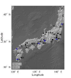
The simulation used transportation data for the bumpers. Based on these data, the location of each site in the network and its demand were configured. The total number of nodes was (Hokkaido and Okinawa were excluded). We assume that the supply sites for the parts were located in Aichi (), Saitama (), and Hiroshima (), Japan, which are known for their high automotive part production. The node locations are shown in Figure 2(a). In Section 5.4, Mt. Fuji was used as an example disaster location to evaluate its robustness. The supply quantity for each supply node was allocated by dividing the demand into three equal parts, ensuring that no fractions were generated, which are given by
where is the total demand. Demand is characterized by where all nodes had positive demand except for the supply node (Figure 2(b)).
Figure 2(c) illustrates the overall network. The edges of the network were intentionally increased to examine their robustness. This network comprised four types of edges.
-
•
Highway: These edges were based on Japan’s major highways. Discounts were applied for continued usage.
-
•
Maritime: These edges represented routes connecting major ports (, , , , , and ) and incurred higher costs than land transportation.
-
•
Local Roads: For edges between nodes less than 300 km apart, half of them were randomly selected to represent this category.
-
•
Storage: These were the self-loop edges, indicating the storage of parts. These self-loops were charged with storage costs.
The cost for highway and local road edges was based on the Euclidean distance, whereas the quadruple of the Euclidean distance was considered for maritime edges. Storage, which were represented by self-loop edges, was allocated a cost corresponding to a Euclidean distance of 10 km. In addition, a discount policy was applied to highways to encourage continuous use: a 20 % and 30 % discounts were offered to traverse two consecutive highway edges and three consecutive edges, respectively. Moreover, switching among different types of edges resulted in an added cost of 20 km. This approach simulated a typical transportation pricing system. In several cases, these cost functions were non-Markov functions.
The simulation was conducted in three steps (). The set of paths excluded paths, including and , and those containing edges with to reduce the computational load. Therefore, the number of elements in the set was , which was denoted as .
| CVX | Merge | Markov | |
|---|---|---|---|
| Transportation cost | |||
| Computation time [s] |
5.3 Imitation Scenario
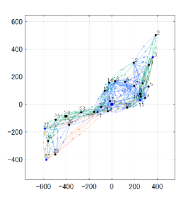
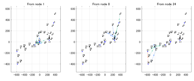
In this section, given an existing logistics plan , we derive a logistics plan that does not significantly change from and improves cost and robustness by solving the I-OT in Problem 6. was intuitively designed to supply from the source node to nearby nodes, while ensuring that the path traversed the fewest possible intermediate nodes, as shown in Fig. 3(a).
For , the resulting transport cost was . Moreover, the minimum-cost logistics plan , that is, the solution to the OT in Problem 1, is shown in Fig. 3(b). The resulting transport cost was . The comparison between and showed that for nodes and , supplying from node was advantageous than supplying from an intuitively closer node . This demonstrated the advantages of solving OT.
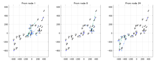
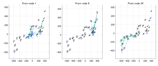
Based on (22), the I-OT solution does not use edges that are not involved in . This implies that if we imitate sparse , various paths are not utilized, and the desired robustness is not achieved. To obtain a robust logistics plan, we employed expressed as
where is the weight. The solution for the I-OT in Scenario 1 is shown in Fig. 3(c) obtained under and using Proposition 15. This result indicates that used various edges while imitating . In addition, reflected the design objective of . Node was supplied via node in the case of , while it was supplied via node in the case of , as in . The resulting transport cost was for . This value was smaller than . Consequently, we were able to realize a plan to minimize cost compared to and utilize a more diverse set of paths, resulting in increased robustness. For improved readability, edges with a usage rate of less than % in the three-step process are not shown in the graph.
In this scenario, both and are non-Markov models. We compared the following three methods for solving the I-OT using non-Markov models.
-
•
Directly solve Eq. (15) using CVX solver (CVX)
-
•
Based on Proposition 15, first, marginalize to obtain and then apply the Sinkhorn iteration (Merge)
-
•
First, approximate by solving Eq. (34) and then apply the Sinkhorn iteration (Markov)
Table 1 represents the results of the comparison. In the case of Markov, a % error was observed; however, as mentioned in Section 4, it had the advantage of obtaining transition matrices for each step. Methods using the Sinkhorn iteration were faster than those employing a general solver. In addition, the calculation time of Merge was thousands of times faster than that of CVX.
5.4 Apriori risk information scenario
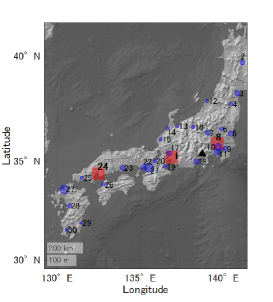
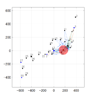
In this section, we assume that there is a priori knowledge of the cost–variation trend at each edge during a disaster. This scenario assumes an eruption of Mt. Fuji. Figure 4 illustrates the expected affected edges. We considered that nodes and completely disrupted all terrestrial transportation routes. In addition, the edges near Mt. Fuji were affected by this disruption. Based on this prior knowledge, is expressed as
| (39) |
This indicates that there were significant cost fluctuations for roads around Mt. Fuji, while there were minimal variations in maritime routes. Figure 5 shows where the edge thickness represents the corresponding entry for .
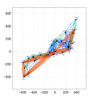
Figure 6 presents the solution for the I-OT in Scenario 2 under and . The strategy of employed marine routes that were expensive but robust. Furthermore, frequently utilized a northerly route, avoiding the area around Mt. Fuji. The resulting total transport cost was .
Assuming a ten-fold increase in the cost of the edges affected by the disaster, as shown in Fig. 4, the total cost of was and that of was . Consequently, was advantageous under these conditions. Table 2 lists the transportation costs to nodes with significant damage. Compared to , exhibits significantly lower cost fluctuations following the disaster. The difference is pronounced in the transportation to node , which uses a northerly route in . These results demonstrate that I-OT effectively utilizes prior knowledge. Notably, node has no impact since all the edges it connects to are damaged.
| Disaster | Before | After | ||
|---|---|---|---|---|
| Node | ||||
| 7 | ||||
| 11 | ||||
| 18 | ||||
6 Conclusion
In this study, we theoretically discussed the following: (1) extension of OT to I-OT; (2) cost robustness obtained using the I-OT solution; (3) properties exhibited in the non-Markovian case. Subsequently, based on their application to logistics, we evaluated the robustness and implications of transportation planning that imitates prior distribution.
The investigation carried out in this work serves as a foundation for further research. In addition to realizing the applicability to larger networks, two topics are currently under investigation. First, there is a mismatch between the demand and the available supply, which can be characterized by unbalanced OT [17]. Second, in relation to Scenario 2, implicitly inferring the uncertainties using the currently adopted transportation plan is important. This is an inverse problem that determines when the optimal solution to Problem 10 with (22) and given is available.
Appendix A Proof of Theorem 8
Appendix B Proof of Theorem 11
Given any probability density function on , consider
| (43) | ||||
Let us introduce a Lagrange multiplier and the following Lagrange function for maximization in (43):
| (44) | ||||
Next, the derivative of with respect to is expressed as
| (45) |
Consequently, the Karush-Kuhn-Tucker condition for the optimal solution is expressed as
| (46) | |||
| (47) | |||
| (48) | |||
| (49) |
Because satisfies , (46) holds only if , for which, (48) or (49) need not be considered. For , we obtain
| (50) |
from (46). By substituting this into (47), we have
for all . Finally, we obtain
| (51) |
The corresponding maximum is expressed as
| (52) | ||||
References
- [1] Michael M. Zavlanos, Magnus B. Egerstedt, and George J. Pappas. Graph-theoretic connectivity control of mobile robot networks. Proceedings of the IEEE, 99(9):1525–1540, 2011.
- [2] Albert-László Barabási. Network science. Philosophical Transactions of the Royal Society A: Mathematical, Physical and Engineering Sciences, 371(1987):20120375, 2013.
- [3] Giuliano Andrea Pagani and Marco Aiello. The power grid as a complex network: A survey. Physica A: Statistical Mechanics and its Applications, 392(11):2688–2700, 2013.
- [4] Tsan-Ming Choi. Guest editorial to the special issue on logistics and supply chain systems engineering. IEEE Transactions on Systems, Man, and Cybernetics: Systems, 50(12):4852–4855, 2020.
- [5] Virginie Gabrel, Cécile Murat, and Aurélie Thiele. Recent advances in robust optimization: An overview. European Journal of Operational Research, 235(3):471–483, 2014.
- [6] Xianlin Zeng, Zhenyi Liu, and Qing Hui. Energy equipartition stabilization and cascading resilience optimization for geospatially distributed cyber-physical network systems. IEEE Transactions on Systems, Man, and Cybernetics: Systems, 45(1):25–43, 2015.
- [7] Yongxin Chen, Tryphon Georgiou, Michele Pavon, and Allen Tannenbaum. Robust transport over networks. IEEE transactions on automatic control, 62(9):4675–4682, 2016.
- [8] Yongxin Chen, Tryphon T Georgiou, Michele Pavon, and Allen Tannenbaum. Efficient robust routing for single commodity network flows. IEEE Transactions on Automatic Control, 63(7):2287–2294, 2017.
- [9] Yilun Shang. Subgraph robustness of complex networks under attacks. IEEE Transactions on Systems, Man, and Cybernetics: Systems, 49(4):821–832, 2019.
- [10] Qing Cai, Sameer Alam, Mahardhika Pratama, and Jiming Liu. Robustness evaluation of multipartite complex networks based on percolation theory. IEEE Transactions on Systems, Man, and Cybernetics: Systems, 51(10):6244–6257, 2021.
- [11] Lijia Ma, Xiao Zhang, Jianqiang Li, Qiuzhen Lin, Maoguo Gong, Carlos A. Coello Coello, and Asoke K. Nandi. Enhancing robustness and resilience of multiplex networks against node-community cascading failures. IEEE Transactions on Systems, Man, and Cybernetics: Systems, 52(6):3808–3821, 2022.
- [12] Shuai Wang, Yaochu Jin, and Ming Cai. Enhancing the robustness of networks against multiple damage models using a multifactorial evolutionary algorithm. IEEE Transactions on Systems, Man, and Cybernetics: Systems, 53(7):4176–4188, 2023.
- [13] Cédric Villani. Topics in Optimal Transportation, volume 58. American Mathematical Soc., 2021.
- [14] E. Schrödinger. Sur la théorie relativiste de l’électron et l’interprétation de la mécanique quantique. Annales de l’institut Henri Poincaré, 2(4):269–310, 1932.
- [15] Christian Léonard. A survey of the schrödinger problem and some of its connections with optimal transport. Discrete and Continuous Dynamical Systems, 34(4):1533–1574, 2014.
- [16] Marco Cuturi. Sinkhorn distances: Lightspeed computation of optimal transport. Advances in neural information processing systems, 26, 2013.
- [17] Gabriel Peyré, Marco Cuturi, et al. Computational optimal transport: With applications to data science. Foundations and Trends® in Machine Learning, 11(5-6):355–607, 2019.
- [18] Benjamin Eysenbach and Sergey Levine. Maximum entropy rl (provably) solves some robust rl problems. arXiv preprint arXiv:2103.06257, 2021.
- [19] Kaito Ito and Kenji Kashima. Entropic model predictive optimal transport over dynamical systems. Automatica, 152:110980, June 2023.
- [20] Koshi Oishi, Yota Hashizume, Tomohiko Jimbo, Hirotaka Kaji, and Kenji Kashima. Resilience evaluation of entropy regularized logistic networks with probabilistic cost. IFAC-PapersOnLine, 56(2):3106–3111, 2023.
- [21] Roy Fox, Ari Pakman, and Naftali Tishby. Taming the noise in reinforcement learning via soft updates. arXiv preprint arXiv:1512.08562, 2015.
- [22] Tuomas Haarnoja, Aurick Zhou, Pieter Abbeel, and Sergey Levine. Soft actor-critic: Off-policy maximum entropy deep reinforcement learning with a stochastic actor. In International conference on machine learning, pages 1861–1870. PMLR, 2018.
- [23] John Schulman, Xi Chen, and Pieter Abbeel. Equivalence between policy gradients and soft q-learning. arXiv preprint arXiv:1704.06440, 2017.
- [24] Takayuki Osa, Joni Pajarinen, Gerhard Neumann, J Andrew Bagnell, Pieter Abbeel, Jan Peters, et al. An algorithmic perspective on imitation learning. Foundations and Trends® in Robotics, 7(1-2):1–179, 2018.
- [25] Jean-Charles Delvenne and Anne-Sophie Libert. Centrality measures and thermodynamic formalism for complex networks. Physical Review E, 83(4):046117, 2011.
- [26] William Parry. Intrinsic markov chains. Transactions of the American Mathematical Society, 112(1):55–66, 1964.
- [27] David Ruelle. Thermodynamic Formalism: The Mathematical Structure of Equilibrium Statistical Mechanics. Cambridge University Press, 2004.
- [28] Dewan Md Zahurul Islam, J Fabian Meier, Paulus T Aditjandra, Thomas H Zunder, and Giuseppe Pace. Logistics and supply chain management. Research in transportation economics, 41(1):3–16, 2013.
- [29] Lu Zhen. A bi-objective model on multiperiod green supply chain network design. IEEE Transactions on Systems, Man, and Cybernetics: Systems, 50(3):771–784, 2020.
- [30] Amirreza Farahani, Laura Genga, and Remco Dijkman. Online multimodal transportation planning using deep reinforcement learning. In 2021 IEEE International Conference on Systems, Man, and Cybernetics (SMC), pages 1691–1698. IEEE, 2021.
- [31] Dan Chen, Xiaoyong Zhang, Dianzhu Gao, Kai Gao, Mengfei Wen, and Zhiwu Huang. Logistics distribution path planning based on fireworks differential algorithm. In 2020 IEEE International Conference on Systems, Man, and Cybernetics (SMC), pages 2797–2802. IEEE, 2020.
- [32] Tryphon T. Georgiou and Michele Pavon. Positive contraction mappings for classical and quantum schrödinger systems. Journal of Mathematical Physics, 56(3), March 2015.
- [33] Paul E. Black. repeated squareing, 2021. https://xlinux.nist.gov/dads/HTML/repeatedSquaring.html.
- [34] Sergey Dashkovskiy, Michael Görges, and Lars Naujok. Autonomous control methods in logistics – a mathematical perspective. Applied Mathematical Modelling, 36(7):2947–2960, 2012.
- [35] Sergey Dashkovskiy, Hamid Reza Karimi, and Michael Kosmykov. A Lyapunov–Razumikhin approach for stability analysis of logistics networks with time-delays. International Journal of Systems Science, 43(5):845–853, 2012.
- [36] Jos F Sturm. Using sedumi 1.02, a matlab toolbox for optimization over symmetric cones. Optimization methods and software, 11(1-4):625–653, 1999.
- [37] Michael Grant and Stephen Boyd. CVX: Matlab software for disciplined convex programming, version 2.1. http://cvxr.com/cvx, March 2014.
- [38] Michael Grant and Stephen Boyd. Graph implementations for nonsmooth convex programs. In V. Blondel, S. Boyd, and H. Kimura, editors, Recent Advances in Learning and Control, Lecture Notes in Control and Information Sciences, pages 95–110. Springer-Verlag Limited, 2008. http://stanford.edu/~boyd/graph_dcp.html.